Light enhancement by quasi-bound states in the continuum in dielectric arrays

Abstract

The article reports on light enhancement by structural resonances in linear periodic arrays of identical dielectric elements. As the basic elements both spheres and rods with circular cross section have been considered. In either case, it has been demonstrated that high-$Q$ structural resonant modes originated from bound states in the continuum enable near-field amplitude enhancement by factor of $10$–$25$ in the red-to-near infrared range in lossy silicon. The asymptotic behavior of the $Q$-factor with the number of elements in the array is explained theoretically by analyzing quasi-bound states propagation bands.

I Introduction

Light trapping by periodic structures is a mainstream idea in thin film photovoltaics Yu et al. (2012); Burresi et al. (2015). The idea dates back to the paper by Sheng, Bloch, and Steplemann who fist proposed to employ a periodic grating substrate in amorphous silicon solar cells Sheng et al. (1983). Since then the periodic structures that diffract light and increase the optical length within the absorbing material have been a subject of numerous publications Heine and Morf (1995); Bermel et al. (2007); Kroll et al. (2008); Wang et al. (2013); Dhindsa et al. (2016). Most remarkably the dielectric gratings have allowed for large enhancement factors Yu et al. (2010) which exceed the fundamental limit for a Lambertian cell Yablonovitch (1982) that holds well only if there is a high density of optical modes in the plane of the structure. At the same time as one approaches the nanophotonic regime the wave nature of light comes into play to call for theoretical approaches taking into account optical resonances Yu et al. (2011).

Due to numerous applications John (2012) trapping, focusing, and concentration of light at the nanoscale have recently emerged as topics of great interest primarily in regard to various plasmonic devices Bartal et al. (2009); Schuller et al. (2010); Fang et al. (2011); Pasquale et al. (2012); Zhang et al. (2015); Jeon et al. (2016); Zhang and Guo (2016) and photonic band-gap structures Chutinan and John (2008); Lin and Povinelli (2009); Wang et al. (2014); Othman et al. (2016). Another promising directions of research is all-dielectric nanophotonics Savelev et al. (2015); Jahani and Jacob (2016) which employs subwavelength dielectric objects, such as e.g. spherical nanoparticles Tribelsky et al. (2015), to tailor the resonant response of the system. Scattering by clusters dielectric spheres has been in research focus for a long time Borghese et al. (1985); Ioannidou et al. (1995); Xu (1995); Merchiers et al. (2007); Wheeler et al. (2010) with high-$Q$ resonant modes in linear Burin et al. (2004); Blaustein et al. (2007); Gozman et al. (2008) as well as circular Burin (2006) arrays predicted a decade ago. Nowadays, thanks to immense progress in manipulating dielectric nanoparticles Fu et al. (2013); Zywietz et al. (2015); Dmitriev et al. (2016), we witness a surge of interest in optical devices based on clusters and arrays of dielectric spheres including subwavelength waveguides Du et al. (2011); Savelev et al. (2014); Bulgakov and Maksimov (2016), optical nanoantenas Krasnok et al. (2012); Fu et al. (2013), and circular oligomers Filonov et al. (2014); Chong et al. (2014).

In this article we consider light enhancement by high-$Q$ structural resonances in linear one-dimensional periodic arrays of identical dielectric elements. In what follows the term structural resonance will be applied to a resonance whose position and width are dictated by the spatial distribution of dielectric elements. Thus, the structural resonances can be contrasted to both natural material resonances and Mie resonances of individual dielectric elements. As the basic elements both spheres and rods with circular cross section will be considered. To achieve high-$Q$ resonances and, consequently, high enhancement factors we propose to tune the parameters of the arrays to bound states in the continuum (BSCs) which are localized states with the eigenfrequency embedded into continuum of propagating solutions Hsu et al. (2016). With the state of the art in the BSC research thoroughly reviewed in the above reference here we simply mention the key experiments on optical BSCs in periodic dielectric structures Plotnik et al. (2011); Lee et al. (2012); Weimann et al. (2013); Chia Wei Hsu et al. (2013); Corrielli et al. (2013); Regensburger et al. (2013).

The BSCs in linear periodic arrays of dielectric cylinders were predicted theoretically in the earlier paper Bulgakov and Sadreev (2014) where the role of the BSCs in wave scattering was also highlighted. More recently, the problem of BSCs in arrays of dielectric rods Yuan and Lu (2016) was revisited with the existence domains in the plane of radius and dielectric constant of the cylinders determined through extensive numerical sumulations. Unlike the guided solution below the line of light Luan and Chang (2006); Du et al. (2009) the qusi-bound modes in the parametric vicinity of a true BSC are resonantly coupled with the freely propagating plane waves to emerge in the scattering cross-section as sharp Fano resonances. In fact the collapse of a Fano resonance is a generic feature inherent to BSCs Kim et al. (1999); Venakides and Shipman (2003); Ladrón de Guevara et al. (2003); Hein et al. (2012) including quasi-BSCs in plasmonics Zou et al. (2004). In the field of optics the above feature has allowed for design of narrow band normal incidence filters Foley et al. (2014); Foley and Phillips (2015); Cui et al. (2016). The BSCs in linear arrays of dielectric spheres were first reported in Bulgakov and Sadreev (2015). As before for arrays of cylinders we contrast the BSCs in arrays of spheres to the guided solutions below the line of light Shore and Yaghjian (2004); Burin et al. (2004); Blaustein et al. (2007); Du et al. (2011); Linton et al. (2013); Savelev et al. (2014). The effect of BSCs on plane wave scattering was considered Bulgakov and Sadreev (2016, 2017) with the trapping of light with orbital angular momentum theoretically predicted. Light enhancement by symmetry protected BSCs in photonic crystal slab was demonstrated in Romano et al. (2015); Mocella and Romano (2015); Yoon et al. (2015). Here, along the same line we propose to employ arrays of finite number of dielectric elements. Although formally BSCs do not exist in finite structures Silveirinha (2014) their traces could be observed in form of high-$Q$ structural resonances Bulgakov and Maksimov (2016) similarly to the traces of photonic band structure emerging in scattering on small clusters of spherical particles Yamilov and Cao (2003).

The article is organized as follows. In Section II we briefly review the BSCs in infinite arrays in dielectric rods. Then we demonstrate structural resonances in the parametric vicinity of BSCs in finite arrays. A simple theory predicting the positions of the structural resonances is proposed. In Section III we show that the same theory applies for the arrays of dielectric spheres. In Section IV we elaborate asymptotic behavior of the $Q$-factor and the enhancement factor for various types of the structural resonances with the increasing number of elements in the array. Finally, we conclude in Section V.

II Quasi-BSCs in arrays of dielectric rods

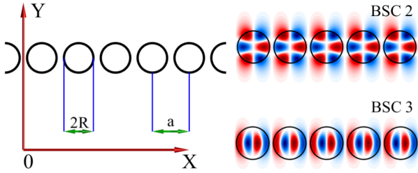
Figure 1: BCSs in arrays of dielectric rods. Left panel: set-up of the array in $x0y$-plane. Right panel: field patterns of $BSCs$ $2$, $3$ from Table 1.

We consider an array of identical dielectric rods of radius $R$ arranged along the $x$-axis with period $a$. The axes of the rods are collinear and aligned with the $z$-axis. The cross-section of the array in $x0y$-plane is shown in Fig. 1 (left panel). The numerical procedure for finding electro-magnetic field in arrays of rods is well-known in literature Yasumoto (2005) and was adapted for BSCs in Bulgakov and Sadreev (2014). Suppose that the array is illuminated by a stationary TM plane wave with its electric vector pointing along the axes of the rods, then according to the above references we have the scattered field inside the rods in the following form

$$E_{z}(x,y)=\sum_{j}\sum_{m=0}^{\infty}c_{m}(j)e^{im\theta_{j}}J_{m}(k_{0}\sqrt{\epsilon}\rho_{j}),$$ (1)

where $j$ enumerates the rods, $\theta_{j},\rho_{j}$ are the local polar coordinates for the $j$ rod, $J_{m}(k_{0}\sqrt{\epsilon}\rho_{j})$ - the Bessel function, $\epsilon$ - the dielectric permittivity, $c_{m}(j)$ - the expansion coefficient, and $k_{0}$ - the frequency. Outside the rods we have a similar expression for the scattering function

$$E_{z}(x,y)=\sum_{j}\sum_{m=0}^{\infty}\overline{c}_{m}(j)e^{im\theta_{j}}H_{m}^{(1)}(k_{0}\rho_{j}),$$ (2)

where $H_{m}^{(1)}(k_{0}\rho_{j})$ is the outgoing Hankel function. The summation over $m$ in Eqs. (1) and (2) runs to infinity. The only approximation in the numerical method is truncation to a finite number of summands in Eqs. (1) and (2). This approximation makes possible to produce a finite interaction matrix of the scattering system and subsequently a finite number of equations for $c_{m}(j),\overline{c}_{m}(j)$ as described in Bulgakov and Sadreev (2014). The method is known to converge rapidly with the number of multipoles Yasumoto (2005). In our computations we used $m=0,1,...,9$ which results in the relative truncation error $10^{-5}$ as defined in Bulgakov and Maksimov (2016). We refer the reader to Bulgakov and Sadreev (2014) for the lengthy equations for amplitudes $c_{m}(j),\overline{c}_{m}(j)$.

II.1 BSCs in infinite arrays

Table 1: BSCs in linear arrays of dielectric cylinders, $\epsilon=15$. SP stands for symmetry protected.

$BSC$	SP	$k_{0}a$	$k_{x}^{0}a$	$R/a$	$\nu$	$\mu$	$a_{\nu}$	$a_{\mu}$
1	Yes	1.8412	0	0.4400	4	2	5.25 $\cdot 10^{-4}$	0.20
2	Yes	3.0758	0	0.4400	2	2	9.6 $\cdot 10^{-3}$	0.05
3	Yes	3.5553	0	0.4400	4	2	2.4 $\cdot 10^{-3}$	0.177
4	Yes	2.3864	0	0.4400	2	2	6.85 $\cdot 10^{-3}$	0.092
5	No	2.8299	0	0.4441	4	2	3.17 $\cdot 10^{-3}$	-0.085
6	No	3.7156	1.6501	0.4400	2	1	5.27 $\cdot 10^{-3}$	-0.0721

In case of infinite arrays the summation over index $j$ in Eqs. (1) and (2) is run from minus to plus infinity. The translation invariance allows to apply the Bloch theorem in the form Yasumoto (2005)

$$c_{m}(j)=c_{m}(0)e^{ik_{x}aj},\ \overline{c}_{m}(j)=\overline{c}_{m}(0)e^{ik_{x}aj},$$ (3)

where $k_{x}$ is the $x$-axis component of the wave vector (Bloch vector). Although the solution (2) is a superposition of outgoing functions it still can be totally decoupled from the far field outgoing waves due to destructive interference between the waves emanating from different rods Bulgakov and Sadreev (2014). In that situation a BSC exists in the system even without the array being illuminated from the far zone. In dependence on $k_{x}$ the BSCs are exceptional points in the quasi-BSCs propagation bands where the imaginary part of the resonant frequency $k_{0}$ turns to zero Bulgakov and Maksimov (2016). In general the asymptotic behavior of the imaginary and real parts of the resonant frequency in the vicinity of a BSCs is described by the following formulas

$$-\Im\{k_{0}a\}=a_{\nu}(k_{x}a-k_{x}^{BSC}a)^{\nu}+\mathcal{O}[(k_{x}a-k_{x}^{BSC}a)^{\nu+2}],$$ (4)

and

$$\Re\{k_{0}a\}=k_{0}^{BSC}a-a_{\mu}{(k_{x}a-k_{x}^{BSC}a)}^{\mu}+\mathcal{O}[(k_{x}a-k_{x}^{BSC}a)^{\mu+1}],$$ (5)

where $k_{0}^{BSC}$ is the BSC frequency, $k_{x}^{BSC}$ - the BSC wave vector along the array axis, and $\nu,\mu$ - the leading coefficient of polynomial expansion Bulgakov and Maksimov (2016). The physical meaning of Eq. (4) is simple; once the system is detuned in $k_{x}$-space from a true BSC point $k_{x}^{BSC}$ the resonance acquires finite life-time given by the inverse of $\Im\{k_{0}\}$. Although the majority of BSCs have $k_{x}^{BSC}=0$, there are also so-called Bloch BSCs which are trapped waves travelling along the array Bulgakov and Sadreev (2014, 2015); Gao et al. (2016). In Table 1 we collect the parameters of six BSCs found for infinite arrays with $\epsilon=15$ (Silicon). The values of $a_{\mu}$ and $a_{\nu}$ in Table 1 were extracted from the data by a polynomial fit. For a typical picture of the band structure of Bloch BSCs the reader is addressed to Bulgakov and Maksimov (2016).

There are two generic types of BSCs in arrays of dielectric rods Bulgakov and Sadreev (2014), symmetry protected, and unprotected by symmetry. Field patterns of symmetry protected $BSCs\ 2,3$ are shown in the left panel in Fig. 1 where one can see that those BCSs are symmetrically mismatched with a plane wave normally incident to the array. The asymptotic behavior of the resonance live-times in the vicinity of a BSC was recently considered by Yuan and Lu Yuan and Lu (2017) who argued that for symmetry protected BSCs the leading term should be $\nu=2$. There were no, however, reliable estimate for $a_{\nu=2}$. In our numerical simulations we found that both $\nu=2$ and $\nu=4$ are possible. In Table 1 we presented the data on four symmetry protected BCSs a couple for each ${\nu=2}$ and ${\nu=4}$. The asymptotic behavior of unprotected BSCs was also considered in Yuan and Lu (2017) with a mathematically rigorous result that for the the standing wave BSCs unprotected by symmetry the leading term is ${\nu=4}$ which is in accordance with our findings for $BSC\ 5$. For Bloch $BSC\ 6$ we found ${\nu=2}$.

II.2 Quasi-BSCs in finite arrays

Next we discuss the the light scattering by various types of quasi-BSCs in finite arrays to highlight the features related to the asymptotic behavior described by Eqs. (4) and (5). The array now consists of $N$ elements and summation over $j$ in Eqs. (1) and (2) runs from $1$ to $N$. In Fig. 2 we present the results of numerical simulations of wave scattering by finite arrays of $N=50$ rods. The parameters $k_{0},k_{x}$ which are the frequency and the $x$-component of an impinging TM plane wave were swept in the parametric vicinity of $BSCs\ 2$ and $3$. Notice that only positive $k_{x}$ were considered for the system is symmetric with respect to the inversion of the $x$-axis. For simplicity the response was recorded as the mean of the absolute value of the leading coefficient in the expansion Eq. (1)

$$\langle|c_{m_{0}}|\rangle=\frac{1}{N}\sum_{j=1}^{N}|c_{m_{0}}(j)|,$$ (6)

where $m_{0}$ is the index of the coefficients $c_{m_{0}}(j)$ in Eq. (1) with the largest absolute value (see top panel in Fig. 2 where $m_{0}=1$).

In both cases one can see ”bright” spots following the asymptotic expression for the real part of the resonant frequency (5). These spots correspond to the structural resonances with the widths of the spots along $k_{0}$-axis proportional to the inverse $Q$-factors which will be considered in Section IV. The nature of the structural resonances could be easily understood by close examination of the upper panel in Fig. 2 where we plotted the expansion coefficients $c_{m}(j)$ for the first resonant spot. One can see from the upper panel in Fig. 2 that the solution is nothing but a sinusoidal standing wave locked between the edges of the array. Thus, to recover the spectrum of the structural resonances one can write down the following condition for the $k_{x}^{(p)}$ of the $p$ structural resonance.

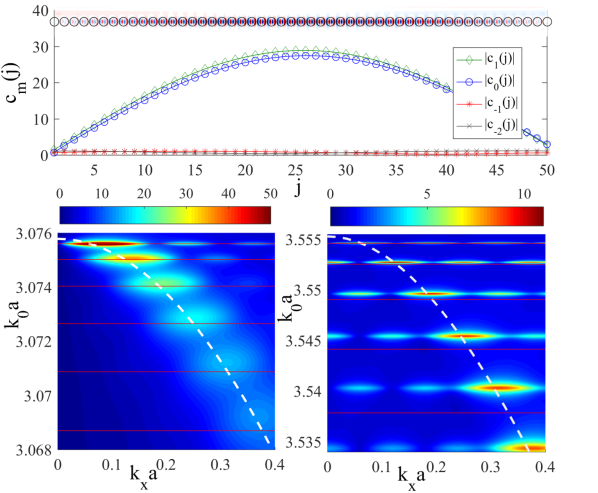
Figure 2: Light scattering in the parametric vicinity of symmetry protected BSCs for dielectric $\epsilon=15$ arrays of rods under illumination by a TM plane wave with unit amplitude. Top panel: expansion coefficients $c_{m}(j)$ vs. the number of the rod $j$ for $N=50$ for $BSC\ 3$. The impinging wave parameters are tuned to the first resonance Eq. (7). The resulting field pattern is shown on top of the subplot. South-west: mean value of the leading coefficient $\langle c_{m_{0}}\rangle$ vs. $k_{0},k_{x}$ in the vicinity of $BSC\ 2$ for $N=50$. South-east: The same for $BSC\ 3$. White dash lines correspond to asymptotic behavior by Eq. (5). The frequencies of structural resonances by Eq. (8) are shown by red horizontal lines.

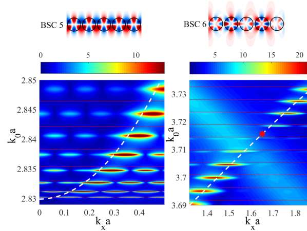
Figure 3: Light scattering in the parametric vicinity of BSCs unprotected by symmetry for dielectric $\epsilon=15$ arrays of rods under illumination by a TM plane wave with unit amplitude. Left panel: Standing wave $BSC\ 5$ unprotected by symmetry; mean value of the leading coefficient $\langle c_{m_{0}}\rangle$ Eq. (6) vs. $k_{0},k_{x}$ in the parametric vicinity of the BSC for $N=50$ rods. The BSC field pattern is shown on top of the subplot. Right panel: the same for Bloch $BSC\ 6$; the star shows the position of $BSC\ 6$ in the parametric space $k_{0},k_{x}$. The BSC field pattern is shown on top of the subplot in form of the real part of the travelling wave amplitude. White dash lines correspond to asymptotic behavior by Eq. (5). The frequencies of structural resonances by Eq. (8) are shown by red horizontal lines.

$$Nak_{x}^{(p)}=\pi p,\ p=1,2,\ldots,.$$ (7)

Then by virtue of Eq. (5) we have

$$\Re\{k_{0}^{(p)}a\}=k_{0}^{BSC}a-a_{\mu}{\left(\frac{\pi p}{N}-k_{x}^{BSC}a\right)}^{\mu},$$ (8)

with $p$ corresponding to the number of half-wavelengths between the edges and the field patterns

$$E_{z}^{(p)}(x)\simeq f(x,y)\sin\left(\frac{\pi px}{Na}\right),$$ (9)

where $f(x,y)=f(x+a,y)$ is the periodic functions corresponding to the BSCs profiles in Fig. 1. Remarkably, despite the BCSs are standing waves the position of the first structural resonance $p=1$ is shifted from $k_{x}=0$ according to Eqs. (7) and (8). The field pattern of the first resonance is shown on top of the upper panel in Fig. 2 to visualize Eq. (9). Notice the resemblance with $BSC\ 3$ in Fig. 1. The resonant frequencies by Eq. (8) are plotted in Fig. 2 by red horizontal lines. One can see that Eq. (8) predicts to a good accuracy the positions of two first resonances $p=1,2$. For $p\geq 3$ the positions of resonances deviate from Eq. (8) due to the higher order terms in the polynomial expansion Eq. (5). This effect could be eliminated by further increase of the length of the array $Na$ with all resonances shifting to the BSC point according to Eq. (8). In addition to the main sequence (8) in Fig. 2 one can see satellite resonant peaks. We speculate that the satellites are due to oscillating coupling of the structural resonances to the impinging wave with the same frequency but a different $k_{x}$ component. Finally, one can see from Fig. 2 that a BSC with $\nu=4$ produces a picture of resonances with smaller high-intensity spots to evidence higher $Q$-factors.

In Fig. 3 we present the results of numerical simulations of wave scattering by finite arrays of $N$ rods in the parametric vicinity of $BSCs\ 5$ and $6$ from Table 1. The field patterns are shown on top of the plot to demonstrate that now the BCSs are not symmetrically mismatched to the normally incident wave. In contrast to symmetry protected ones the BSCs of this sort are much more difficult to come by for they always require some adjustment of either radius $R$ or Bloch vector $k_{x}$ to occur through an involved interference picture Bulgakov and Sadreev (2014). One can see from Fig. 3 that the response function (6) demonstrates features very similar to those in Fig. 2 with structural resonances emerging at frequencies by Eq. (8). Again for standing wave $BSC\ 5$ we see that only position of two first structural resonances are accurately predicted by Eq. (8). Another source of error could be additional phase accumulated in reflection from the edge of the array not accounted for by Eq. (7). Also notice that for Bloch $BSC\ 6$ the structural resonances are equidistant with $a_{\mu=1}$ being the group velocity according to Eq. (5).

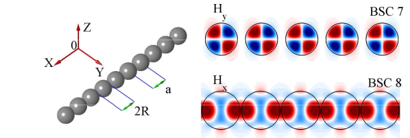
Figure 4: BCS in arrays of dielectric spheres. Left panel: set-up of the array. Right panel: The field patterns in form of $H_{y}$ component for $BSC\ 7$ and $H_{x}$ component for $BSC\ 8$ in $x0z$-plane.

III Quasi-BSCs in arrays of dielectric spheres

The system under scrutiny is schematically depicted in Fig. 4. For arrays dielectric spheres we will follow the recipes from Bulgakov and Sadreev (2015) where the method by Linton, Zalipaev, and Thompson Linton et al. (2013) was adapted for finding BSCs. The parameters of two BSCs, one symmetry protected, and one unprotected by symmetry are given in Table 2. In the above referenced method the magnetic and electric vectors could be found in terms of Mie coefficients $a_{n}^{m}(j),b_{n}^{m}(j)$. For instance, outside the spheres one has for the the scattered EM field electric vector ${\bf E}({\bf r})$

$${\bf E}({\bf r})=\sum_{j}\sum^{\infty}_{n=m^{*}}\left[a_{n}^{m}(j){\bf M}^{m}_{n}({\bf r}-{\bf r}_{j})+b_{n}^{m}(j){\bf N}^{m}_{n}({\bf r}-{\bf r}_{j})\right],$$ (10)

where $j$ the number of the sphere in the array, ${\bf r}_{j}$ - the coordinates of the $j$ sphere, m - azimuthal number, $m^{*}=max(1,m)$, and ${\bf N}^{m}_{n}({\bf r}),{\bf M}^{m}_{n}({\bf r})$ are spherical vector harmonics Stratton (1941). Again in the case of infinite arrays we have according to the Bloch theorem

$$a_{n}^{m}(j)=a_{n}^{m}(0)e^{ik_{x}aj},\ b_{n}^{m}(j)=b_{n}^{m}(0)e^{ik_{x}aj}.$$ (11)

In this paper we restrict ourself we with $m=0$, though BSCs with higher orbital angular momentum are possible Bulgakov and Sadreev (2016, 2017). The field patterns of BSCs from Table 2 are shown in the left panel in Fig. 4. Notice that $BSC$ 7 in Table 2 is a wave of the TM-type which means $H_{x}$=0, and $b_{n}^{0}(j)=0$ Bulgakov and Sadreev (2015). In contrast $BSC$ 8 is a TE-wave with $E_{x}$=0, and $b_{n}^{0}(j)=0$.

Table 2: BSCs in linear arrays of dielectric spheres, $\epsilon=15$. SP stands for symmetry protected.

$BSC$	SP	$k_{0}a$	$k_{x}^{0}a$	$R/a$	$\nu$	$\mu$	$a_{\nu}$	$a_{\mu}$
7	Yes	3.6022	0	0.400	2	2	1.366 $\cdot 10^{-2}$	0.010
8	No	2.9280	0	0.485	4	2	0.1818 $\cdot 10^{-2}$	-0.0793

Let us now consider the resonant response of finite array with $N$ spheres. Despite the similarity of Eq. (10) to Eqs. (1) and (2) the numerical method is now computationally much more expensive due to the necessity to evaluate lattice sums with involved special functions Linton et al. (2013). Though limited to the power of a desktop computer we can still circumvent the computational difficulties by recollecting the resonant picture from the previous section. First by using Eq. (8) one can obtain the frequencies of a structural resonance. Then the response function Eq. (6) is computed numerically only in dependance on $k_{x}$ with coefficients $a_{n}^{0}(j),b_{n}^{0}(j)$ from Eq. (10) now used instead of $c_{m}(j)$ in Eq. (6). The results for $BSC\ 8$ from Table 2 under illumination by a TE-polarized plane wave of unit amplitude are plotted in Fig. 5. Again one can see sinusoidal standing waves similar to Fig. 2. Notice that for the second resonance $p=2$ in Eq. (8) we intentionally chose $N=200$ to eliminated the errors due to the higher order terms in Eq. (5). The response function against $k_{x}$ for $k_{0}$ corresponding to the first and the second resonances Eq. (8) is also demonstrated in the insets in Fig. 5. Again one observes an oscillatory dependance with a pronounced maximum corresponding to Eq. (7) as in Figs. 2,3. For $BSC\ 7$ the same results were observed under illumination by a TM-polarized plane wave.

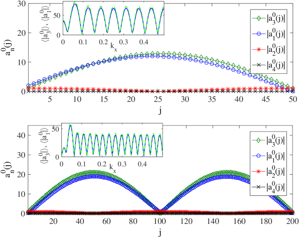
Figure 5: Light scattering by structural resonances in the parametric vicinity of $BSC\ 8$ in arrays of dielectric spheres. Top panel: the leading coefficients in Eq. (10) for the first structural resonance $N=50$. Bottom panel: the leading coefficients in Eq. (10) for the second structural resonance $N=200$. The insets show the response function Eq. (6) evaluated with leading Mie coefficients $a^{0}_{1}(j),a^{0}_{3}(j)$ against the Bloch wave vector $k_{x}$.

IV Light enhancement

Bearing in mind the structure of resonant response of finite arrays we can now address the question of how many dielectric elements in the array are needed to observe the effect of light enhancement in a realistic experiment with two figures of merit being the quality and enhancement factors. Before proceeding to the assessment of those quantities we would like to mention that so far all results were presented in dimensionless units to emphasize that the model is applicable to silicon dielectric arrays both in the visible as well as in the near infrared where the real part of the dielectric constant varies insignificantly with the frequency of light Vuye et al. (1993); Green and Keevers (1995). It should be noted, however, that the imaginary part in the same range can vary by orders of magnitude. Thus, one may expect that the effect of light enhancement will be limited by the material losses in silicon.

IV.1 Q-factors

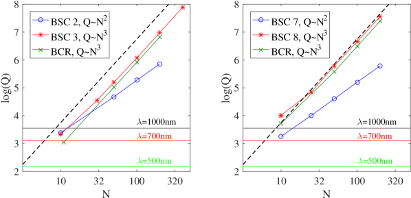
Figure 6: Q-factors for structural resonances against the number of dielectric elements $N$. Left panel: arrays of rods; BCR with $k_{0}a=2.8908,k_{x}a=\pi,R/a=0.44$. Right panel: arrays of spheres; BCR with $k_{0}a=2.052,k_{x}a=\pi,R/a=0.40$. The black dash line shows the best result found in Blaustein et al. (2007). The horizontal lines show the limits due to material losses in silicon.

Here we use the standard definition of the $Q$-factor

$$Q=\frac{\omega}{\gamma},$$ (12)

where $\omega$ is the resonance frequency, and $\gamma$ is the resonance width, both quantities extracted from the scattering data described in the previous sections Figs. 2,5. The $Q$-factors against the number of dielectric elements in the array for the first ($p=1$ in Eq. (8)) structural resonance of $BSCs\ 2,3,7$, and $8$ are plotted in Fig. 6. As expected from Eqs. (4) and (7) the $Q$-factor for resonances with $\nu=2$ scales as $Q\sim N^{2}$, however, for $\nu=4$ we observed $Q\sim N^{3}$ which, seemingly, contradicts our theoretical predictions. The contradiction can be resolved by noticing that Eq. (4) only describes one specific mechanism of the radiation losses equally applicable for both finite and infinite arrays, namely, the radiation from the sides of the arrays due to detuning from the true BSC point in the parametric space. In the case of finite arrays there is another radiation mechanism due to the losses at the edges as the wave bounces between them to form the sinusoidal resonant mode shape Eq. (9). Obviously, for the guided modes below the line of light that would be the only possible radiation mechanism because the radiative losses at the sides are forbidden by total internal reflection. In fact, the scaling law for the edge radiation is already obtained in Blaustein et al. (2007) where the authors demonstrated that the $Q$-factor scales as $Q\sim N^{3}$. Thus, one can conclude that in case of $\nu=4$ the radiative losses at the sides are suppressed by the radiative losses at the edges resulting in the scaling law for resonances formed by guided modes below the line of light Blaustein et al. (2007).

In accordance with our findings we can now define side-coupled resonances with $Q\sim N^{2}$ for BSCs with $\nu=2$, and a wider class of edge-coupled resonances with $Q\sim N^{3}$ which encompasses both BSCs with $\nu=4$ as well as the below continuum resonances (BCRs). Now it is instructive to compare our results with the $Q$-factors for the BCRs. To do that in Fig. 6 we plot the $Q$-factors for two BCR one for rods and spheres each. The parameters of the BCRs are given in the caption to Fig. 6. One can see that both $\nu=2$ BSCs and BCR demonstrate a similar dependance against $N$.

Finally, let us access the role of the material losses. The $Q$-factor limits were estimated based on the data on the imaginary part of refractive index at $\lambda=500,700$nm by Vuye et al. (1993), and at $\lambda=1000$nm by Green and Keevers (1995). One can easily see from Fig. 6 that $Q\approx 10^{3}$–$10^{4}$ resonances can be observed with silicon in the red-to-near-infrared range for arrays of $N\approx 10$–$15$ elements.

IV.2 Enhancement factors

We define the enhancement factor $F$ as the average of the square root of the field intensity $I({\bf r})$ within the volume $V=\pi R^{2}Na$ (or area $2RNa$) containing the whole of the finite array divided by the square root of the field intensity carried by the incoming wave $I_{0}$.

$$F=\frac{1}{\sqrt{I_{0}}V}\int_{V}d{\bf r}\sqrt{I({\bf r})}.$$ (13)

Although according to Eq. (9) the EM-field varies significantly in the vicinity of the array the enhancement factor $F$ defined through Eq. (13) is able to quantify to what extent the field amplitude is enhanced by resonant scattering. In Fig. 7 we plot the enhancement factors for the first ($p=1$ in Eq. (8)) structural resonance of $BSCs\ 2,3,7$, and $8$ as well as the BCRs used in Fig. 6. The arrays were illuminated with a plane wave with frequency equal to the frequency of the resonance. The $k_{x}$ - component of the incident wave each time was tuned to the maximum response which in case of BSC were given by Eq. (7). For BCR the maximum response was found at the strict normal incidence. One can see that only for the side-coupled resonances $BSC$ 2,7 the enhancement factor is nicely fit by the expected dependence $F\sim\sqrt{Q}\sim N$ Yoon et al. (2015). Notice that in the above reference the enhancement was defined through intensity rather that amplitude. For the edge-coupled resonances we were unable to produce a simple polynomial fit which is probably due to the residual side-coupling emerging through the specific excitation of the resonance by a plane wave. More interesting, though, is that the side-coupled resonances $BSC$ 2,7 produce significantly larger enhancement factors than the edge-coupled ones, and hence should be opted for as the operating resonances for light enhancement. In lossy silicon the limits for the enhancement factor of the side-coupled resonances will be placed at the same arrays lengths as were found from Fig. 6 for the Q-factors. Thus, comparing Fig.7 against Fig.6 one can conclude that the amplitude enhancement factors $F\approx 10$–$25$ can be achieved with arrays of $10$–$15$ silicon subwavelength nanospheres in the red-to-near-infrared range with the side-coupled resonances.

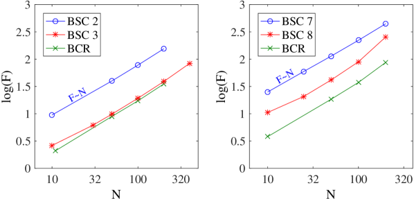
Figure 7: The enhancement factor of dielectric arrays. Left panel: arrays of rods. Right panel: arrays of spheres.

V Conclusion

We demonstrated that the traces of bound states in the continuum in one-dimensional dielectric arrays can be observed as a specific family of high-$Q$ resonances specified by the number of half-wavelengths placed between the edges of the arrays. Two types of such resonances were identified. The edge-coupled resonances possessing a higher $Q$-factor are similar to the below continuum resonances known earlier Blaustein et al. (2007) to have the $Q$-factor scaling law as $Q\sim N^{3}$ with $N$ being the number of elements in the array. In contract, the side-coupled resonances with lesser $Q$-factors have the scaling law $Q\sim N^{2}$. Interestingly, it is the side-coupled resonances related to BSCs that under illumination by a plane wave demonstrate higher enhancement factors providing a platform for light enhancement by finite dielectric arrays with the parameters tuned to a BSC.

It should be pointed out that in terms of both the $Q$-factor asymptotics and compactness our set-up is no match to ultra-compact Fabry-Perot cavities Velha et al. (2007) where the $Q$-factor scales exponentially with the number of periods in Bragg mirrors. Those asymptotics, however, are hard to achieve in silicon nonophotonics as the subwavelength spheres are scaled down in size to the visible wavelength where the material losses become significant. Our simulations show that in the red-to-near-infrared range the $Q$-factors of $10^{3}$–$10^{4}$ and the amplitude enhancement factors $F\approx 10$–$25$ can be achieved with arrays of $10$–$15$ silicon subwavelength nanospheres.

In contrast to familiar Fano resonances Kim et al. (1999); Venakides and Shipman (2003); Ladrón de Guevara et al. (2003); Hein et al. (2012) the structural resonances in finite systems are shown to generate a complicated picture in the resonant response to illumination by a plane wave. With the frequency of the impinging wave tuned to the structural resonance we observed the oscillating behavior of the enhanced EM-field amplitude under variation of the wave vector component directed along the array. In real systems the effect of finiteness will be always eventually obscured by material losses. One may expect that with the increase of the length of the array the many pronounced resonances will merge into a Fano feature. We speculate that this picture could be explained by a properly set coupled mode theory Suh et al. (2004) based on analytical estimates for resonant frequencies and mode shapes obtained in this paper. Along with asymptotic scaling law for edge-coupled resonances enhancement factor this constitutes a goal for future studies.

The bound states in the continuum were recently employed for engineering high-$Q$ resonators for compact nanophotonic lasers Kodigala et al. (2017) providing access to new coherent sources with intriguing topological properties for optical trapping, biological imaging, and quantum communication. To provide useful guidelines for practical implementations of structures supporting the bound states the effects of both structural fluctuations Ni et al. (2017) and substrate coupling Sadrieva et al. (2017) have recently been considered. As it was mentioned earlier in the introduction the BSCs are only allowed in infinite systems Silveirinha (2014) so that in design of BSC-based devices the researchers will always be bound with residual radiation losses. We believe that our model of the BSC related structural resonances sheds some light onto important aspects of emerging BSC nanophotonics Hsu et al. (2016); Rybin and Kivshar (2017).

Funding

This work was supported by Ministry of Education and Science of Russian Federation (state contract N 3.1845.2017) and RFBR grant 16-02-00314.

References

- Yu et al. (2012) M. Yu, Y.-Z. Long, B. Sun, and Z. Fan, Nanoscale 4, 2783 (2012).
- Burresi et al. (2015) M. Burresi, F. Pratesi, F. Riboli, and D. S. Wiersma, Advanced Optical Materials 3, 722 (2015).
- Sheng et al. (1983) P. Sheng, A. N. Bloch, and R. S. Stepleman, Applied Physics Letters 43, 579 (1983).
- Heine and Morf (1995) C. Heine and R. H. Morf, Applied Optics 34, 2476 (1995).
- Bermel et al. (2007) P. Bermel, C. Luo, L. Zeng, L. C. Kimerling, and J. D. Joannopoulos, Optics Express 15, 16986 (2007).
- Kroll et al. (2008) M. Kroll, S. Fahr, C. Helgert, C. Rockstuhl, F. Lederer, and T. Pertsch, physica status solidi (a) 205, 2777 (2008).
- Wang et al. (2013) C. Wang, S. Yu, W. Chen, and C. Sun, Scientific Reports 3, 1025 (2013).
- Dhindsa et al. (2016) N. Dhindsa, J. Walia, M. Pathirane, I. Khodadad, W. S. Wong, and S. S. Saini, Nanotechnology 27, 145703 (2016).
- Yu et al. (2010) Z. Yu, A. Raman, and S. Fan, Optics Express 18, A366 (2010).
- Yablonovitch (1982) E. Yablonovitch, J. Opt. Soc. Am. 72, 899 (1982).
- Yu et al. (2011) Z. Yu, A. Raman, and S. Fan, Applied Physics A 105, 329 (2011).
- John (2012) S. John, Nature Materials 11, 997 (2012).
- Bartal et al. (2009) G. Bartal, G. Lerosey, and X. Zhang, Physical Review B 79, 201103(R) (2009).
- Schuller et al. (2010) J. A. Schuller, E. S. Barnard, W. Cai, Y. C. Jun, J. S. White, and M. L. Brongersma, Nature Materials 9, 193 (2010).
- Fang et al. (2011) Z. Fang, Q. Peng, W. Song, F. Hao, J. Wang, P. Nordlander, and X. Zhu, Nano Letters 11, 893 (2011).
- Pasquale et al. (2012) A. J. Pasquale, B. M. Reinhard, and L. Dal Negro, ACS Nano 6, 4341 (2012).
- Zhang et al. (2015) J. Zhang, Z. Guo, C. Ge, W. Wang, R. Li, Y. Sun, F. Shen, S. Qu, and J. Gao, Optics Express 23, 17883 (2015).
- Jeon et al. (2016) T. Y. Jeon, D. J. Kim, S.-G. Park, S.-H. Kim, and D.-H. Kim, Nano Convergence 3, 18 (2016).
- Zhang and Guo (2016) A. Zhang and Z. Guo, Optik - International Journal for Light and Electron Optics 127, 2861 (2016).
- Chutinan and John (2008) A. Chutinan and S. John, Physical Review A 78, 023825 (2008).
- Lin and Povinelli (2009) C. Lin and M. L. Povinelli, Optics Express 17, 19371 (2009).
- Wang et al. (2014) K. X. Wang, Z. Yu, V. Liu, A. Raman, Y. Cui, and S. Fan, Energy & Environmental Science 7, 2725 (2014).
- Othman et al. (2016) M. A. K. Othman, F. Yazdi, A. Figotin, and F. Capolino, Physical Review B 93, 024301 (2016).
- Savelev et al. (2015) R. S. Savelev, S. V. Makarov, A. E. Krasnok, and P. A. Belov, Opt. Spectrosc. 119, 551 (2015).
- Jahani and Jacob (2016) S. Jahani and Z. Jacob, Nature Nanotechnology 11, 23 (2016).
- Tribelsky et al. (2015) M. I. Tribelsky, J.-M. Geffrin, A. Litman, C. Eyraud, and F. Moreno, Scientific Reports 5, 12288 (2015).
- Borghese et al. (1985) F. Borghese, P. Denti, R. Saija, G. Toscano, and O. I. Sindoni, Il Nuovo Cimento D 6, 545 (1985).
- Ioannidou et al. (1995) M. P. Ioannidou, N. C. Skaropoulos, and D. P. Chrissoulidis, J. Opt. Soc. Am. A 12, 1782 (1995).
- Xu (1995) Y.-l. Xu, Applied Optics 34, 4573 (1995).
- Merchiers et al. (2007) O. Merchiers, F. Moreno, F. González, and J. M. Saiz, Physical Review A 76, 043834 (2007).
- Wheeler et al. (2010) M. S. Wheeler, J. S. Aitchison, and M. Mojahedi, J. Opt. Soc. Am. B 27, 1083 (2010).
- Burin et al. (2004) A. L. Burin, H. Cao, G. C. Schatz, and M. A. Ratner, J. Opt. Soc. Am. B 21, 121 (2004).
- Blaustein et al. (2007) G. S. Blaustein, M. I. Gozman, O. Samoylova, I. Y. Polishchuk, and A. L. Burin, Optics Express 15, 17380 (2007).
- Gozman et al. (2008) M. Gozman, I. Polishchuk, and A. Burin, Physics Letters A 372, 5250 (2008).
- Burin (2006) A. L. Burin, Physical Review E 73, 066614 (2006).
- Fu et al. (2013) Y. H. Fu, A. I. Kuznetsov, A. E. Miroshnichenko, Y. F. Yu, and B. Luk’yanchuk, Nature Communications 4, 1527 (2013).
- Zywietz et al. (2015) U. Zywietz, M. K. Schmidt, A. B. Evlyukhin, C. Reinhardt, J. Aizpurua, and B. N. Chichkov, ACS Photonics 2, 913 (2015).
- Dmitriev et al. (2016) P. A. Dmitriev, D. G. Baranov, V. A. Milichko, S. V. Makarov, I. S. Mukhin, A. K. Samusev, A. E. Krasnok, P. A. Belov, and Y. S. Kivshar, Nanoscale 8, 9721 (2016).
- Du et al. (2011) J. Du, S. Liu, Z. Lin, J. Zi, and S. T. Chui, Physical Review A 83, 035803 (2011).
- Savelev et al. (2014) R. S. Savelev, A. P. Slobozhanyuk, A. E. Miroshnichenko, Y. S. Kivshar, and P. A. Belov, Physical Review B 89, 035435 (2014).
- Bulgakov and Maksimov (2016) E. N. Bulgakov and D. N. Maksimov, Optics Letters 41, 3888 (2016).
- Krasnok et al. (2012) A. E. Krasnok, A. E. Miroshnichenko, P. A. Belov, and Y. S. Kivshar, Optics Express 20, 20599 (2012).
- Filonov et al. (2014) D. S. Filonov, A. P. Slobozhanyuk, A. E. Krasnok, P. A. Belov, E. A. Nenasheva, B. Hopkins, A. E. Miroshnichenko, and Y. S. Kivshar, Applied Physics Letters 104, 021104 (2014).
- Chong et al. (2014) K. E. Chong, B. Hopkins, I. Staude, A. E. Miroshnichenko, J. Dominguez, M. Decker, D. N. Neshev, I. Brener, and Y. S. Kivshar, Small 10, 1985 (2014).
- Hsu et al. (2016) C. W. Hsu, B. Zhen, A. D. Stone, J. D. Joannopoulos, and M. Soljačić, Nature Reviews Materials 1, 16048 (2016).
- Plotnik et al. (2011) Y. Plotnik, O. Peleg, F. Dreisow, M. Heinrich, S. Nolte, A. Szameit, and M. Segev, Physical Review Letters 107, 183901 (2011).
- Lee et al. (2012) J. Lee, B. Zhen, S.-L. Chua, W. Qiu, J. D. Joannopoulos, M. Soljačić, and O. Shapira, Physical Review Letters 109, 067401 (2012).
- Weimann et al. (2013) S. Weimann, Y. Xu, R. Keil, A. E. Miroshnichenko, A. Tünnermann, S. Nolte, A. A. Sukhorukov, A. Szameit, and Y. S. Kivshar, Physical Review Letters 111, 240403 (2013).
- Chia Wei Hsu et al. (2013) Chia Wei Hsu, B. Zhen, J. Lee, S.-L. Chua, S. G. Johnson, J. D. Joannopoulos, and M. Soljačić, Nature 499, 188 (2013).
- Corrielli et al. (2013) G. Corrielli, G. Della Valle, A. Crespi, R. Osellame, and S. Longhi, Physical Review Letters 111, 220403 (2013).
- Regensburger et al. (2013) A. Regensburger, M.-A. Miri, C. Bersch, J. Näger, G. Onishchukov, D. N. Christodoulides, and U. Peschel, Physical Review Letters 110, 223902 (2013).
- Bulgakov and Sadreev (2014) E. N. Bulgakov and A. F. Sadreev, Physical Review A 90, 053801 (2014).
- Yuan and Lu (2016) L. Yuan and Y. Y. Lu, Journal of Physics B: Atomic, Molecular and Optical Physics 50, 05LT01 (2016).
- Luan and Chang (2006) P.-G. Luan and K.-D. Chang, Optics Express 14, 3263 (2006).
- Du et al. (2009) J. Du, S. Liu, Z. Lin, J. Zi, and S. T. Chui, Physical Review A 79, 205436 (2009).
- Kim et al. (1999) C. S. Kim, A. M. Satanin, Y. S. Joe, and R. M. Cosby, Physical Review B 60, 10962 (1999).
- Venakides and Shipman (2003) S. Venakides and S. P. Shipman, SIAM Journal on Applied Mathematics 64, 322 (2003).
- Ladrón de Guevara et al. (2003) M. Ladrón de Guevara, F. Claro, and P. Orellana, Phys. Rev. B 67, 195335 (2003).
- Hein et al. (2012) S. Hein, W. Koch, and L. Nannen, J. Fluid Mech. 692, 257 (2012).
- Zou et al. (2004) S. Zou, N. Janel, and G. C. Schatz, J. Chem. Phys. 120, 10871 (2004).
- Foley et al. (2014) J. M. Foley, S. M. Young, and J. D. Phillips, Physical Review B 89, 165111 (2014).
- Foley and Phillips (2015) J. M. Foley and J. D. Phillips, Optics Letters 40, 2637 (2015).
- Cui et al. (2016) X. Cui, H. Tian, Y. Du, G. Shi, and Z. Zhou, Scientific Reports 6, 36066 (2016).
- Bulgakov and Sadreev (2015) E. N. Bulgakov and A. F. Sadreev, Physical Review A 92, 023816 (2015).
- Shore and Yaghjian (2004) R. A. Shore and A. D. Yaghjian, Traveling electromagnetic waves on linear periodic arrays of small lossless penetrable spheres, Tech. Rep. (DTIC Document, 2004).
- Linton et al. (2013) C. Linton, V. Zalipaev, and I. Thompson, Wave Motion 50, 29 (2013).
- Bulgakov and Sadreev (2016) E. N. Bulgakov and A. F. Sadreev, Physical Review A 94, 033856 (2016).
- Bulgakov and Sadreev (2017) E. Bulgakov and A. Sadreev, Advanced Electromagnetics 6, 1 (2017).
- Romano et al. (2015) S. Romano, I. Rendina, and V. Mocella, in 2015 AEIT International Annual Conference (AEIT) (2015).
- Mocella and Romano (2015) V. Mocella and S. Romano, Physical Review B 92, 155117 (2015).
- Yoon et al. (2015) J. W. Yoon, S. H. Song, and R. Magnusson, Scientific Reports 5, 18301 (2015).
- Silveirinha (2014) M. G. Silveirinha, Physical Review A 89, 023813 (2014).
- Yamilov and Cao (2003) A. Yamilov and H. Cao, Physical Review B 68, 085111 (2003).
- Yasumoto (2005) K. Yasumoto, Electromagnetic theory and applications for photonic crystals (CRC Press, 2005).
- Gao et al. (2016) X. Gao, C. W. Hsu, B. Zhen, X. Lin, J. D. Joannopoulos, M. Soljačić, and H. Chen, Scientific Reports 6, 31908 (2016).
- Yuan and Lu (2017) L. Yuan and Y. Y. Lu, Physical Review A 95, 023834 (2017).
- Stratton (1941) J. A. Stratton, Electromagnetic theory, edited by L. A. DuBridge (McGraw-Hill Book Company, Inc., 1941).
- Vuye et al. (1993) G. Vuye, S. Fisson, V. Nguyen Van, Y. Wang, J. Rivory, and F. Abelès, Thin Solid Films 233, 166 (1993).
- Green and Keevers (1995) M. A. Green and M. J. Keevers, Progress in Photovoltaics: Research and Applications 3, 189 (1995).
- Velha et al. (2007) P. Velha, E. Picard, T. Charvolin, E. Hadji, J. Rodier, P. Lalanne, and D. Peyrade, Optics Express 15, 16090 (2007).
- Suh et al. (2004) W. Suh, Z. Wang, and S. Fan, IEEE Journal of Quantum Electronics 40, 1511 (2004).
- Kodigala et al. (2017) A. Kodigala, T. Lepetit, Q. Gu, B. Bahari, Y. Fainman, and B. Kanté, Nature 541, 196 (2017).
- Ni et al. (2017) L. Ni, J. Jin, C. Peng, and Z. Li, Optics Express 25, 5580 (2017).
- Sadrieva et al. (2017) Z. F. Sadrieva, I. S. Sinev, K. L. Koshelev, A. Samusev, I. V. Iorsh, O. Takayama, R. Malureanu, A. A. Bogdanov, and A. V. Lavrinenko, ACS Photonics 4, 723 (2017).
- Rybin and Kivshar (2017) M. Rybin and Y. Kivshar, Nature 541, 164 (2017).