On the Spectral Efficiency and Fairness in Full-Duplex Cellular Networks

Abstract

To increase the spectral efficiency of wireless networks without requiring full-duplex capability of user devices, a potential solution is the recently proposed three-node full-duplex mode. To realize this potential, networks employing three-node full-duplex transmissions must deal with self-interference and user-to-user interference, which can be managed by frequency channel and power allocation techniques. Whereas previous works investigated either spectral efficient or fair mechanisms, a scheme that balances these two metrics among users is investigated in this paper. This balancing scheme is based on a new solution method of the multi-objective optimization problem to maximize the weighted sum of the per-user spectral efficiency and the minimum spectral efficiency among users. The mixed integer non-linear nature of this problem is dealt by Lagrangian duality. Based on the proposed solution approach, a low-complexity centralized algorithm is developed, which relies on large scale fading measurements that can be advantageously implemented at the base station. Numerical results indicate that the proposed algorithm increases the spectral efficiency and fairness among users without the need of weighting the spectral efficiency. An important conclusion is that managing user-to-user interference by resource assignment and power control is crucial for ensuring spectral efficient and fair operation of full-duplex networks.

I Introduction

Due to recent advancements in antenna and digital baseband technologies, as well as radio-frequency/analog interference cancellation techniques, in-band full-duplex (FD) transmissions appear as a viable alternative to traditional half-duplex (HD) transmission modes [1]. The in-band FD transmission mode can almost double the spectral efficiency of conventional HD wireless transmission modes, especially in the low transmit power domain [1, 2]. However, due to the increasing demand for supporting the transmission of large data quantities in scarce spectrum scenarios [1, 3], and thanks to the continued advances in self-interference (SI) cancellation technologies, FD is being considered as a technology component beyond small cell and short range communications [4, 5].

A viable introduction of FD technology in cellular networks consists in making the base station (BS) FD-capable, while letting the user equipments operate in HD mode. This transmission mode is termed three node full-duplex (TNFD) [1], in which only one of the three nodes (i.e., two UEs and the cellular BS) must have FD and SI suppression capability. In a TNFD cellular network, the FD-capable BS transmits to its receiving UE, while receiving from another UE on the same frequency channel.

An example of a cellular network employing TNFD with two UEs pairs is illustrated in Figure 1. Note that apart from the inherently present SI, FD operation in a cellular network must also deal with the UE-to-UE interference, indicated by the red dotted lines between $\text{UE}_{1}$-$\text{UE}_{4}$ and $\text{UE}_{2}$-$\text{UE}_{3}$. The level of UE-to-UE interference depends on the UEs locations and propagation environments and their transmission powers. To mitigate the negative effects of the interference on the spectral efficiency of the system, coordination mechanisms are needed  [5]. Two key elements of such mechanisms are UE pairing and power allocation, that together determine which UEs are scheduled for simultaneous uplink (UL) and downlink (DL) transmissions, and at which power UL and DL UEs will transmit or receive. Consequently, it is crucial to design efficient and fair medium access control protocols and physical layer procedures capable of supporting adequate coordination mechanisms.

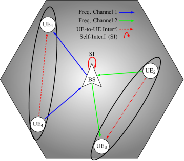
Figure 1: An example of cellular network employing FD with two UEs pairs. The BS selects pairs $\text{UE}_{1}$-$\text{UE}_{4}$ and $\text{UE}_{2}$-$\text{UE}_{3}$, represented by the ellipses, and jointly schedules them for FD transmission by allocating frequency channels in the UL and DL. To mitigate the UE-to-UE interference, it is advantageous to co-schedule DL/UL users for FD transmission that are far apart, such as $\text{UE}_{1}$-$\text{UE}_{2}$ and $\text{UE}_{3}$-$\text{UE}_{4}$.

A typical and natural objective for many physical layer procedures for FD cellular networks proposed in the literature is to maximize the sum spectral efficiency [6, 7]. The authors in [6] consider a joint subcarrier and power allocation problem, but without taking into account the UE-to-UE interference. The work reported in [7] considers the application of TNFD transmission mode in a cognitive femto-cell scenario with bidirectional transmissions from UEs, and develops sum-rate optimal resource allocation and power control algorithms.

Another important objective is to improve the fairness and per-user quality of service (QoS) of FD cellular networks, as emphasized in  [2, 1, 8, 9]. In our previous work, we proposed a weighted sum spectral efficiency maximization, where the weights represent path-loss compensation and are thus related to the rate distribution and fairness in the system [2]. The results showed that FD cellular networks can outperform current HD mode if appropriate SI cancellation and pairing schemes are employed. A heterogeneous statistical QoS provisioning framework, focusing on the bidirectional FD link case without considering the implications of TNFD transmissions is developed in [8]. The work in [1] emphasizes the importance of fairness and that it may degrade by a factor of two compared with HD communications. However, the authors do not provide power control and channel allocation schemes that are developed with such objectives in mind. In contrast, our previous work [9] formulated the maximization of the minimum spectral efficiency problem and proposed a max-min fair power control and channel allocation solution.

However, the interplay between weighted sum spectral efficiency maximization and fairness for FD cellular networks has not been studied. Therefore, in this work we aim to fill this research gap by proposing a multi-objective optimization problem to maximize simultaneously both the weighted sum spectral efficiency and the minimum spectral efficiency of all users. Such an optimization problem poses technical challenges that are markedly different from those investigated in our previous works [9, 2]. In particular, we develop an original and new solution approach based on the use of the scalarization technique to convert the multi-objective into a single-objective mixed integer nonlinear programming (MINLP) problem that considers jointly user pairing and UL/DL power control. Due to the complexity of the MINLP problem proposed, our novel solution approach relies on Lagrangian duality and the associated centralized algorithm based on the dual problem. This centralized solution is tested in a realistic system simulator that indicates that the solution is near-optimal, and increases the sum spectral efficiency and fairness among the users. An important feature of the proposed solution is that there is no need to consider weights in the sum spectral efficiency as done in previous works from the literature [2]. This is advantageous, because defining the weights in a weighted sum objective function is typically cumbersome and difficult in practice.

The numerical results also indicate that measuring and taking into account UE-to-UE interference is crucial for both overall spectral efficiency and fairness. When UE-to-UE interference is neglected, as in [6], the results are approximately as good as using random assignment and equal power allocation among all users.

II System Model and Problem Formulation

II-A System Model

We consider a hexagonal single-cell cellular system in which the BS is FD capable, while the UEs served by the BS are HD capable, as illustrated by Figure 1. In the figure, the BS is subject to SI, and the UEs in the UL ($\text{UE}_{2}$ and $\text{UE}_{4}$) cause UE-to-UE interference to co-scheduled UEs in the DL, that is to $\text{UE}_{3}$ and $\text{UE}_{1}$ respectively. The number of UEs in the UL and DL is denoted by $I$ and $J$, respectively, which are constrained by the total number of frequency channels in the system $F$, i.e., $I\leq F$ and $J\leq F$. The sets of UL and DL users are denoted by $\mathcal{I}=\{1,\ldots,I\}$ and $\mathcal{J}=\{1,\ldots,J\}$, respectively.

In this paper, we assume that fading is slow and frequency flat, which is an adequate model from the perspective of power control in existing and forthcoming cellular networks [10, 11]. Let $G_{ib}$ denote the path gain between transmitter UE $i$ and the BS, $G_{bj}$ denote the path gain between the BS and the receiver UE $j$, and $G_{ij}$ denote the interfering path gain between the UL transmitter UE $i$ and the DL receiver UE $j$.

The vector of transmit power levels in the UL by UE $i$ is denoted by $\mathbf{p^{u}}=[P_{1}^{u}\ldots P_{I}^{u}]$, whereas the DL transmit powers by the BS is denoted by $\mathbf{p^{d}}=[P_{1}^{d}\ldots P_{J}^{d}]$. We define $\beta$ as the SI cancellation coefficient to take into account the residual SI that leaks to the receiver. Then, the SI power at the receiver of the BS is $\beta P_{j}^{d}$ when the transmit power is $P_{j}^{d}$.

As illustrated in Figure 1, the UE-to-UE interference depends heavily on the geometry of the co-scheduled UL and DL users, which in turn is determined by the co-scheduling or pairing of UL and DL users on the available frequency channels. Therefore, UE pairing is a key function of the system. To capture the pairing of UE pairs, we define the pairing matrix, $\mathbf{X}\in\{0,1\}^{I\times J}$, such that

$$x_{ij}=\begin{cases}1,&\text{if the UL $\text{UE}_{i}$ is paired with the DL $\text{UE}_{j}$},\\ 0,&\text{otherwise.}\end{cases}$$

The signal-to-interference-plus-noise ratio (SINR) at the BS of transmitting user $i$ and the SINR at the receiving user $j$ of the BS are given by

$$\gamma_{i}^{u}=\frac{P_{i}^{u}G_{ib}}{\sigma^{2}+\sum_{j=1}^{J}x_{ij}P_{j}^{d}\beta},\;\gamma_{j}^{d}=\frac{P_{j}^{d}G_{bj}}{\sigma^{2}+\sum_{i=1}^{I}x_{ij}P_{i}^{u}G_{ij}},$$ (1)

respectively, where $x_{ij}$ in the denominator of $\gamma_{i}^{u}$ accounts for the SI at the BS, whereas $x_{ij}$ in the denominator of $\gamma_{j}^{d}$ accounts for the UE-to-UE interference caused by $\text{UE}_{i}$ to $\text{UE}_{j}$, and $\sigma^{2}$ is the noise power. The achievable spectral efficiency for each user is given by the Shannon equation for the UL and DL as $C_{i}^{u}=\log_{2}(1+\gamma_{i}^{u})$ and $C_{j}^{d}=\log_{2}(1+\gamma_{j}^{d})$, respectively.

In addition to the spectral efficiency, we weight the achievable spectral efficiencies by constant weights, which are denoted by $\alpha_{i}^{u}$ and $\alpha_{j}^{d}$, respectively. The purpose of these weights is to allow the system designer to choose between the commonly used sum rate maximization and important fairness related criteria such as the well known path loss compensation typically employed in the power control of cellular networks [12]. The weights $\alpha_{i}^{u}$ and $\alpha_{j}^{d}$ can account for sum rate maximization by setting $\alpha_{i}^{u}=\alpha_{j}^{d}=1$, or for path loss compensation by setting $\alpha_{i}^{u}=G_{ib}^{-1}$ and $\alpha_{j}^{d}=G_{bj}^{-1}$.

II-B Problem Formulation

Our goal is to maximize both the weighted sum spectral efficiency and the minimum spectral efficiency of all users, jointly considering the assignment of UEs in the UL and DL (pairing). This multi-objective optimization problem can be transformed to a single-objective optimization problem through the scalarization technique [13, Sec. 4.7.4]. We choose $(1-\mu)$ as the weight for the weighted sum spectral efficiency and $\mu$ for the minimum spectral efficiency, where $\mu\in[0,1]$. Specifically, we formulate the problem as

$$\underset{\mathbf{X},\mathbf{p}^{u},\mathbf{p}^{d}}{\text{maximize}}\quad \Big{(}1-\mu\Big{)}\Big{(}\sum\nolimits_{i=1}^{I}\alpha_{i}^{u}C_{i}^{u}+\sum\nolimits_{j=1}^{J}\alpha_{j}^{d}C_{j}^{d}\Big{)}$$

$$+\mu\;\min_{\begin{subarray}{c}\forall i,j\end{subarray}}\{C_{i}^{u},C_{j}^{d}\}$$ (2a)

subject to $$P_{i}^{u}\leq P_{\text{max}}^{u},\;\forall\;i,$$ (2b)

$$P_{j}^{d}\leq P_{\text{max}}^{d},\;\forall\;j,$$ (2c)

$$\sum\nolimits_{i=1}^{I}x_{ij}\leq 1,\;\forall\;j,$$ (2d)

$$\sum\nolimits_{j=1}^{J}x_{ij}\leq 1,\;\forall\;i,$$ (2e)

$$x_{ij}\in\{0,1\},\;\forall\;i,j.$$ (2f)

The optimization variables are $\mathbf{p}^{u}$, $\mathbf{p}^{d}$ and $\mathbf{X}$. Constraints (2b) and (2c) limit the transmit powers, whereas constraints (2d)-(2e) assure that only one UE in the DL can share the frequency resource with a UE in the UL and vice-versa. For the sake of clarity, we denote the solution to problem (2) as P-OPT.

Problem (2) belongs to the category of MINLP, which is known for its high complexity and computational intractability [14]. To find a near-to-optimal solution to problem (2) we establish an original approach using the dual problem, as described in Section III. However, the complexity of the dual problem solution might be prohibitive in practical cellular systems, which motivates the reformulation of the dual problem in Section IV, whose proposed solution in Algorithm 1 is denoted C-HUN.

III Solution Approach Based on Lagrangian Duality

III-A Problem Transformation

As a first step of solving problem (2), we consider the standard equivalent hypograph [13, Sec. 3.1.7] form of problem (2), where the new variable $t$ and two more constraints are introduced. Note that the hypograph simplifies the problem formulation, because it allows to use a linear function of the variable $t$ instead of the minimum between two nonlinear functions with the other variables.

$$\underset{\mathbf{X},\mathbf{p}^{u},\mathbf{p}^{d},t}{\text{maximize}} \textstyle\Big{(}1-\mu\Big{)}\Big{(}\sum\nolimits_{i=1}^{I}\alpha_{i}^{u}C_{i}^{u}+\sum\nolimits_{j=1}^{J}\alpha_{j}^{d}C_{j}^{d}\Big{)}+\mu t$$

subject to $$C_{i}^{u}\geq t,\forall i,$$ (3a)

$$C_{j}^{d}\geq t,\forall j$$ (3b)

$$\text{Constraints\leavevmode\nobreak\ \eqref{eq:power_ul}-\eqref{eq:binary_x}},$$

where $t>0$ is an additional variable with respect to (2). Notice that problem (3), similarly to problem (2), is a MINLP.

III-B Solution for $\mathbf{X}$ and $\mathbf{p}^{u},\mathbf{p}^{d}$

From problem (3), we form the partial Lagrangian function by taking into account constraints (3a)-(3b) and ignoring the integer (2d)-(2f) and power allocation constraints (2b)-(2c). To account for these constraints, it is assumed that $\mathbf{X}\in\mathcal{X}$ and $\mathbf{p}^{u},\mathbf{p}^{d}\in\mathcal{P}$, where $\mathcal{X}$ and $\mathcal{P}$ are sets in which the assignment constraints and power allocation constraints are fulfilled, respectively. The Lagrange multipliers associated with problem (3) are $\boldsymbol{\lambda}^{u},\;\boldsymbol{\lambda}^{d}$, where the superscripts $u$ and $d$ denote UL and DL, and the vectors have dimensions of $I\times 1$ and $J\times 1$, respectively.

The partial Lagrangian is a function of the Lagrange multipliers and the optimization variables $\mathbf{X},\mathbf{p}^{u},\mathbf{p}^{d}$ as follows:

$$L(\boldsymbol{\lambda}^{u},\boldsymbol{\lambda}^{d},\mathbf{X},\mathbf{p}^{u},\mathbf{p}^{d}) \triangleq-\Big{(}1-\mu\Big{)}\Big{(}\sum_{i=1}^{I}\alpha_{i}^{u}C_{i}^{u}+\sum_{j=1}^{J}\alpha_{j}^{d}C_{j}^{d}\Big{)}$$

$$-\mu t+\sum\nolimits_{i=1}^{I}\lambda_{i}^{u}\Big{(}t-C_{i}^{u}\Big{)}+\sum\nolimits_{j=1}^{J}\lambda_{j}^{d}\Big{(}t-C_{j}^{d}\Big{)}.$$ (4)

It is useful to rewrite the partial Lagrangian function as

$$L(\boldsymbol{\lambda}^{u},\boldsymbol{\lambda}^{d},\mathbf{X},\mathbf{p}^{u},\mathbf{p}^{d}) =t\Big{(}\sum\nolimits_{i=1}^{I}\lambda_{i}^{u}+\sum\nolimits_{j=1}^{J}\lambda_{j}^{d}-\mu\Big{)}$$

$$-\sum_{i=1}^{I}\Big{(}\lambda_{i}^{u}+(1-\mu)\alpha_{i}^{u}\Big{)}C_{i}^{u}-\sum_{j=1}^{J}\Big{(}\lambda_{j}^{d}+(1-\mu)\alpha_{j}^{d}\Big{)}C_{j}^{d}.$$ (5)

Let $g(\boldsymbol{\lambda}^{u},\boldsymbol{\lambda}^{d})$ denote the dual function obtained by minimizing the partial Lagrangian function (III-B) with respect to the variables $\mathbf{X},\mathbf{p}^{u},\mathbf{p}^{d}$. Thus,

$$g(\boldsymbol{\lambda}^{u},\boldsymbol{\lambda}^{d}) =\underset{\scriptscriptstyle\mathbf{X}\in\mathcal{X}\;\mathbf{p}^{u},\mathbf{p}^{d}\in\mathcal{P}}{\inf}L(\boldsymbol{\lambda}^{u},\boldsymbol{\lambda}^{d},\mathbf{X},\mathbf{p}^{u},\mathbf{p}^{d})$$ (6a)

$$g(\boldsymbol{\lambda}^{u},\boldsymbol{\lambda}^{d})= \underset{\scriptscriptstyle\mathbf{X}\in\mathcal{X}\;\mathbf{p}^{u},\mathbf{p}^{d}\in\mathcal{P}}{\inf}\textstyle\Big{[}\sum_{i}q_{i}^{u}(\mathbf{X},\mathbf{p}^{u},\mathbf{p}^{d})+$$

$$g(\boldsymbol{\lambda}^{u},\boldsymbol{\lambda}^{d})= \sum\nolimits_{j}q_{j}^{d}(\mathbf{X},\mathbf{p}^{u},\mathbf{p}^{d})\Big{]}, \underset{i}{\sum}\lambda_{i}^{u}+\underset{j}{\sum}\lambda_{j}^{d}=\mu$$ if

$$g(\boldsymbol{\lambda}^{u},\boldsymbol{\lambda}^{d})= -\infty,$$ otherwise, (6b)

where it follows from equality (6b) that the linear function $t\big{(}\sum_{i=1}^{I}\lambda_{i}^{u}+\sum_{j=1}^{J}\lambda_{j}^{d}-\mu\big{)}$ is lower bounded when it is identically zero, and

$$q_{i}^{u}(\mathbf{X},\mathbf{p}^{u},\mathbf{p}^{d}) \triangleq-\Big{(}\lambda_{i}^{u}+(1-\mu)\alpha_{i}^{u}\Big{)}C_{i}^{u},$$ (7a)

$$q_{j}^{d}(\mathbf{X},\mathbf{p}^{u},\mathbf{p}^{d}) \triangleq-\Big{(}\lambda_{j}^{d}+(1-\mu)\alpha_{j}^{d}\Big{)}C_{j}^{d}.$$ (7b)

The infimum of the dual function (6b) is obtained when the SINR of the UL-DL pairs is maximized. We can therefore write an initial solution for the assignment $x_{ij}$ as follows:

$$x_{ij}^{\star}=\begin{cases}1,&\text{if }(i,j)=\underset{i,j}{\operatorname*{arg\,max}}\;\Big{(}q_{i}^{u}+q_{j}^{d}\Big{)}\\ 0,&\text{otherwise,}\end{cases}$$ (8)

where, for simplicity, we denote an ordinary pair of UL-DL users as $(i,j)$. With the assignment solution given by (8) and recalling that $x_{ij}\in\mathcal{X}$, an UL user can be uniquely associated with a DL user. However, $x_{ij}^{\star}$ is still tied through the SINRs in the UL and DL, $\gamma_{i}^{u}$ and $\gamma_{j}^{d}$, respectively. With this, the solution for the assignment is still complex and – through $q_{i}^{u}$ and $q_{j}^{d}$ – is intertwined with the optimal power allocation.

Recall that from Eq. (6b) we must find the infimum of the sum between terms in Eqs. (7). Thus, with the initial solution for the assignment problem of finding $\mathbf{X}$, we can now evaluate the power allocation assuming that the pairs $(i,j)$ are already formed. The power allocation problem is formulated as follows:

$$\underset{\mathbf{p}^{u},\mathbf{p}^{d}}{\text{maximize}}\quad \sum\nolimits_{i=1}^{I}\Big{(}\lambda_{i}^{u}+(1-\mu)\alpha_{i}^{u}\Big{)}C_{i}^{u}+$$

$$+\sum\nolimits_{j=1}^{J}\Big{(}\lambda_{j}^{d}+(1-\mu)\alpha_{j}^{d}\Big{)}C_{j}^{d}$$ (9a)

subject to $$\mathbf{p}^{u},\mathbf{p}^{d}\in\mathcal{P},$$ (9b)

where the minimization of negative sums is converted to the maximization of positive sums. From the results of [10], it follows that the optimal transmit power allocation will have either $P_{i}^{u}$ or $P_{j}^{d}$ equal to $P_{\text{max}}^{u}$ or $P_{\text{max}}^{d}$, given that $i$ and $j$ share a frequency channel and form a pair. Therefore, the optimal power allocation is found within the corner points of $(P_{i}^{u},P_{j}^{d})$: $(0,P_{\text{max}}^{d})$, $(P_{\text{max}}^{u},0)$ or $(P_{\text{max}}^{u},P_{\text{max}}^{d})$. If a user (either in the UL or DL) is not sharing the resource, i.e., assigned to a frequency channel alone, then its transmit power is simply $P_{\text{max}}^{u}$ or $P_{\text{max}}^{d}$. With the assignment and power allocation solutions, we now need to find the optimal Lagrange multipliers $\boldsymbol{\lambda}^{u}$ and $\boldsymbol{\lambda}^{d}$.

III-C Dual Problem Solution

We need to find the Lagrangian multipliers $\lambda_{i}^{u}$ and $\lambda_{j}^{d}$, which also appear in the objective function of problem (9). Given the optimal power allocation problem (9), the dual function can be written as

$$g(\boldsymbol{\lambda}^{u},\boldsymbol{\lambda}^{d}) =-\sum_{i=1}^{I}\lambda_{i}^{u}C_{i}^{u}-\sum_{j=1}^{J}\lambda_{j}^{d}C_{j}^{d}-h(C_{i}^{u},C_{j}^{d}),$$ (10)

where the term $h(C_{i}^{u},C_{j}^{d})$ is the weighted sum of UL and DL spectral efficiencies, which are independent of $\lambda_{i}^{u}$ and $\lambda_{j}^{d}$, and do not impact the dual problem. Therefore, the dual problem of (9) can be formulated as

$$\underset{\boldsymbol{\lambda}^{u},\;\boldsymbol{\lambda}^{u}}{\text{minimize}} \sum\nolimits_{i=1}^{I}\lambda_{i}^{u}C_{i}^{u}+\sum\nolimits_{j=1}^{J}\lambda_{j}^{d}C_{j}^{d}$$ (11a)

subject to $$\sum\nolimits_{i=1}^{I}\lambda_{i}^{u}+\sum\nolimits_{j=1}^{J}\lambda_{j}^{d}=\mu,$$ (11b)

$$\lambda_{i}^{u},\;\lambda_{j}^{d}\geq 0,\forall i,j,$$ (11c)

where the maximization of negative sums is converted to the minimization of positive sums. The dual problem (11) is a Linear Programming (LP) problem in the variables $\lambda_{i}^{u}$ and $\lambda_{j}^{d}$.

It is convenient to rewrite the dual problem (11) in the standard LP form as [15, Sec. 4.2]:

$$\underset{\boldsymbol{\lambda}}{\text{minimize}} \mathbf{c}^{T}\boldsymbol{\lambda}$$ (12a)

subject to $$\mathbf{a}\boldsymbol{\lambda}=b,$$ (12b)

$$\boldsymbol{\lambda}\geq 0,$$ (12c)

where $\mathbf{c}=[C_{1}^{u}\;\ldots\;C_{I}^{u}\;C_{1}^{d}\;\ldots\;C_{J}^{d}]^{T}$, the variable vector is $\boldsymbol{\lambda}=[\lambda_{1}^{u}\;\ldots\;\lambda_{I}^{u}\;\lambda_{1}^{d}\;\ldots\;\lambda_{j}^{d}]^{T}$, the constraint vector $\mathbf{a}=\mathbf{1}^{T}$, and $b=\mu$. Since $\mathbf{a}$ has rank 1, we can separate the components of $\boldsymbol{\lambda}$ into two subvectors [15, Sec. 4.3], one consisting of $(I+J-1)$ nonbasic variables $\lambda_{N}$ (all of which are zero), and another consisting of 1 basic variable $\lambda_{B}$, which is equal to $b$. Therefore, we have a single nonzero $\lambda_{B}$, either in the UL or DL, whose index $B$ corresponds to the user with minimum spectral efficiency.

Therefore, using the results on the solution to the assignment problem (8), the optimal power allocation problem (9) from Section III-B, the dual problem (11) can be solved by checking exhaustively which pair of UL and DL users jointly solve Eq. (8), where the power allocation for each pair is within the corner points of set $\mathcal{P}$. Nevertheless, for a large number of users, this exhaustive search solution might not be practical due to the large number of iterations. Because of this property, we will reformulate the dual problem and propose a centralized solution in Section IV.

IV Centralized Solution based on the Lagrangian Dual Problem

IV-A Insights from the Dual Problem

In Section III-C, we showed that the dual problem (11) maximizes the user with minimum spectral efficiency in the system. To this end, we can initially set one $\lambda$ equal to $\mu$ and exhaustively check which one maximizes the power allocation problem (9). However, such exhaustive solution demands large number of iterations that depend on the number of simultaneously served UL and DL users. Consequently, such solution is not viable in practical systems.

Notice that the minimum spectral efficiency that a user can achieve is 0, because of the binary power control solution in problem (9). Therefore, whenever one user in the pair is not transmitting (has zero power), the $\lambda$ associated with that user will be nonzero, which leads to the non-uniqueness of $\lambda$. To reduce the complexity on the search of the nonzero $\lambda$, we assume that for each pair there is a $\lambda$ which equals $\mu$, whose index corresponds to the user with the minimum spectral efficiency of that pair.

IV-B Centralized Solution to Reformulated Dual Problem

Based on the reasoning on the non-uniqueness of $\lambda$ above and using the results from Section III, we reformulate the dual problem (11) to solve the assignment in Eq. (8). We propose a solution that aims at jointly maximizing the sum of the minimum spectral efficiency of the UL-DL pairs and the sum spectral efficiency. To this end, we rewrite the solution in Eq. (8) as an assignment problem given by

$$\underset{\mathbf{X}}{\text{maximize}}\quad \sum\nolimits_{i=1}^{I}\sum\nolimits_{j=1}^{J}s_{ij}x_{ij}$$ (13a)

subject to $$\sum\nolimits_{i=1}^{I}x_{ij}=1,\;\forall j,$$ (13b)

$$\sum\nolimits_{j=1}^{J}x_{ij}=1,\;\forall i,$$ (13c)

$$x_{ij}\in\{0,1\},\;\forall i,j,$$ (13d)

where the matrix $\mathbf{S}=[s_{ijf}]\in\mathbb{R}^{I\times J}$ can be understood as the benefit of pairing UL user $i$ with DL user $j$. It is given by $s_{ij}\!=(1-\mu)(\alpha_{i}^{u}C_{i}^{u}+\alpha_{j}^{d}C_{j}^{d})+\mu\min\{C_{i}^{u},C_{j}^{d}\}$ for a pair $(i,j)$ assigned to the same frequency. Constraint (13b) ensures that the DL users are associated with exactly one UL user. Similarly, constraint (13c) ensures that each UL user must be associated with a DL user.

Computing the optimal assignment as given by problem (13) requires checking $(I+J)!$ assignments [16, Section 1]. Alternatively, the Hungarian algorithm can be used in a fully centralized manner [16, Section 3.2], which has worst-case complexity of $O\Big{(}(I+J)^{3}\Big{)}$. Algorithm 1 summarizes the steps to solve problem (13) using the Hungarian algorithm. The inputs to Algorithm 1 are all the path gain between UL users, DL users and the BS. The BS runs Algorithm 1 and acquires or estimates the channel gains, which are measured and feedback by the served UEs using signalling mechanisms standardized by 3${}^{\text{rd}}$ Generation Partnership Project (3GPP) [11]. The most challenging measure to obtain is the UE-to-UE interference path gain for the pair $(i,j)$, but due to recent advances in 3GPP for device-to-device communications, this measurement can be obtained by sidelink transmissions and receptions  [17].

Algorithm 1 Centralized Algorithm at the BS

1:  Input: $\alpha_{i}^{u},\;\alpha_{i}^{u},\;G_{ibf},\;G_{bjf},\;G_{ijf},\;\beta,\;P_{\text{max}}^{u},\;P_{\text{max}}^{d}$

2:  for $i=1$ to $I$  do

3:    for $j=1$ to $J$  do

4:       Evaluate the corner point $(P_{i}^{u},P_{j}^{d})$ that maximizes $s_{ij}=(1-\mu)(\alpha_{i}^{u}C_{i}^{u}+\alpha_{j}^{d}C_{j}^{d})+\mu\min\{C_{i}^{u},C_{j}^{d}\}$

5:    end for

6:  end for

7:  With $s_{ij}$, evaluate the optimal assignment using Hungarian algorithm

8:  Output: $\mathbf{X},\mathbf{p}^{u},\mathbf{p}^{d}$

Once all inputs are available, the optimal power allocation for all possible pairs needs to be evaluated (see line 4). Algorithm 1 evaluates which corner point the pair $(i,j)$ belongs to, and stores $s_{ij}$ for later use. With $s_{ij}$ at hand, the assignment problem (13) can be solved by using the Hungarian algorithm  [16, Section 3.2] (see line 7). The outputs of the algorithm (see line 8) are the assignment matrix $\mathbf{X}$, and the optimal power allocation vectors $\mathbf{p}^{u},\,\mathbf{p}^{d}$. The complexity of Algorithm 1 hinges on creating the matrix $\mathbf{S}$, which, recall, has a complexity $O(3IJ)$, and on the Hungarian algorithm, which has worst-case complexity of $O\Big{(}(I+J)^{3}\Big{)}$.

V Numerical Results and Discussion

In this section we consider a single cell system operating in the urban micro environment [18]. The maximum number of frequency channels is $F=25$ that corresponds to the number of available frequency channel blocks in a 5 MHz LTE system [18]. The total number of served UE are $I+J=8$ and $I+J=50$, where we assume that $I=J$. We set the weights $\alpha_{i}^{u}$ and $\alpha_{j}^{d}$ based on either sum rate maximization (SR), or path loss compensation rule (PL). For SR, we set $\alpha_{i}^{u}=\alpha_{j}^{d}=1$, whereas for PL we set $\alpha_{i}^{u}=G_{ib}^{-1}$ and $\alpha_{j}^{d}=G_{bj}^{-1}$. The parameters of the simulations are set according to Table I.

To evaluate the performance of the proposed centralized solution in Algorithm 1, we use the RUdimentary Network Emulator (RUNE) as a basic platform for system simulations and extended it to FD cellular networks [19]. The RUNE FD simulation tool allows to generate the environment of Table I and to perform Monte Carlo simulations using either an exhaustive search algorithm to solve problem (2) or the centralized Hungarian solution.

Table I: Simulation parameters

Parameter	Value
Cell radius	$100\,\mathrm{m}$
Number of UL UEs $[I=J]$	$[4\;25]$
Monte Carlo iterations	$400$
Carrier frequency	$2.5\,\mathrm{GHz}$
System bandwidth	$5\,\mathrm{MHz}$
Number of freq. channels $[F]$	$[4\;25]$
line of sight (LOS) path-loss model	$34.96+22.7\log_{10}(d)$
non-line of sight (NLOS) path-loss model	$33.36+38.35\log_{10}(d)$
Shadowing st. dev. LOS and NLOS	$3\,\mathrm{dB}$ and $4\,\mathrm{dB}$
Thermal noise power $[\sigma^{2}]$	$-116.4\,\mathrm{dBm}$/channel
SI cancelling level $[\beta]$	$-100$ $\,\mathrm{dB}$
Max power $[P^{u}_{\text{max}}]=[P^{d}_{\text{max}}]$	$24\,\mathrm{dBm}$

Initially, we compare the optimality gap between the exhaustive search solution of problem (2), named P-OPT, and our proposed solution using Algorithm 1 with the optimal power allocation and the centralized Hungarian algorithm for the assignment, named C-HUN. In the following, we compare our proposed centralized solution with a basic FD solution with random assignment and equal power allocation for UL and DL users, named herein as R-EPA. In addition, we also consider a modified version of C-HUN that does not take into account UE-to-UE interference, named C-NINT. The motivation for C-NINT is to analyse how important the consideration of UE-to-UE interference is to the fairness and the sum spectral efficiency of the system.

Figure 2 shows the objective function in Eq. (2a) between P-OPT and C-HUN as a measure of the optimality gap. We assume a small system with reduced number of users, 4 UL and DL users, and frequency channels, where we assume $\mu\!=\![0.1\;0.5\;0.9]$ and with $\alpha_{i}^{u}\!=\!\alpha_{j}^{d}\!=\!1$ to represent SR. Moreover, we consider a SI cancelling level of $\beta\!=$$-100\,\mathrm{dB}$.

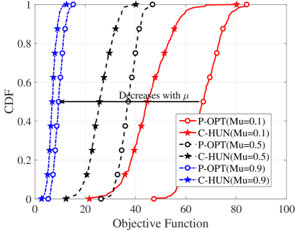
Figure 2: CDF of the objective function in Eq. (2a) for different values of $\mu$. We notice that the optimality gap between P-OPT and C-HUN decreases with $\mu$. Moreover, the objective function decreases with $\mu$, which is expected because of the reduction of the term with sum spectral efficiency.

Notice that the difference between the P-OPT and C-HUN decreases when $\mu$ increases. For instance, for $\mu\!=\!0.1$ the relative difference between P-OPT and C-HUN is approximately $33\,\mathrm{\%}$, whereas for $\mu\!=\!0.9$ this difference decreases to $26\,\mathrm{\%}$. In addition, the value of the objective function also decreases with $\mu$ because the term with the sum spectral efficiency also decreases.

Figure 3 shows Jain’s fairness index for the proposed solution C-HUN, the modified solution C-NINT that does not consider UE-to-UE interference, and the basic benchmark solution R-EPA. We assume a system fully loaded with 25 UL, DL users, and frequency channels, where we analyse the impact of the solutions for different weights of $\alpha_{i}^{u}$ and $\alpha_{j}^{d}$, which are denoted SR for sum rate maximization, and PL for path-loss compensation. The value of $\mu$ is 0.9, which implies that we aim at a more fair scenario. The SI cancelling level is $-100\,\mathrm{dB}$, i.e., $\beta=$$-100\,\mathrm{dB}$.

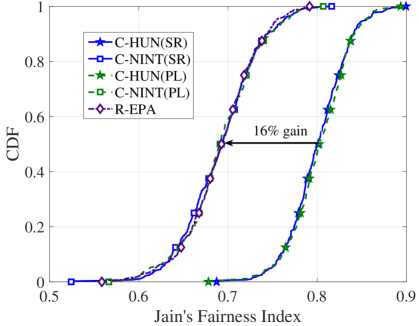
Figure 3: CDF of Jain’s fairness index for $\mu\!=0.9$ and different different weights of $\alpha_{i}^{u}$ and $\alpha_{j}^{d}$. Notice that C-HUN achieves similar performance for SR and PL, which implies that for high values of $\mu$ SR is enough to achieve high fairness in the system. Also, C-NINT is as good as a R-EPA, but with higher complexity.

We notice that the difference between SR and PL for the proposed solution C-HUN is negligible, which implies that we can achieve similar levels of fairness without using weights on $\alpha_{i}^{u}$ and $\alpha_{j}^{d}$. Conversely, there is a gain of approximately $16\,\mathrm{\%}$ between C-HUN and C-NINT at the 50-th percentile irrespectively of the weights on $\alpha_{i}^{u}$ and $\alpha_{j}^{d}$. In addition, there is practically no difference between C-NINT and R-EPA, which implies that using advanced solutions for pairing and power allocation without considering UE-to-UE interference bring losses to the system, and is as good as doing everything randomly and setting maximum power to all users. Thus, our proposed solution C-HUN is able to improve fairness in the system by approximately $16\,\mathrm{\%}$ in comparison with the benchmark solution R-EPA.

Figure 4 shows the sum spectral efficiency of the system for C-HUN, C-NINT, and R-EPA, where we assume the same parameters as the ones used for Figure 3.

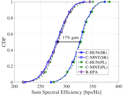
Figure 4: CDF of the sum spectral efficiency for all users. We notice that C-HUN is also able to improve the sum spectral efficiency with respect to C-NINT and R-EPA. Moreover, C-HUN with SR has practically the same performance as PL, implying that the weights on $\alpha_{i}^{u}$ and $\alpha_{j}^{d}$ are not necessary for high values of $\mu$.

As before, the difference between SR and PL for the proposed solution C-HUN is negligible, implying that also for the sum spectral efficiency there is practically no difference between using weights on $\alpha_{i}^{u}$ and $\alpha_{j}^{d}$. As noted earlier, there is a gain of approximately $17\,\mathrm{\%}$ between C-HUN and C-NINT at the 50-th percentile for SR weights on $\alpha_{i}^{u}$ and $\alpha_{j}^{d}$. Also, note that C-NINT for SR is slightly outperformed by R-EPA, and for PL, C-NINT is as good as R-EPA. This clearly shows that UE-to-UE interference needs to be taken into account if the system wants to maximize sum spectral efficiency. Therefore, C-HUN improves the sum spectral efficiency of the system by approximately $17\,\mathrm{\%}$ in comparison with the benchmark solution R-EPA. Overall, we notice that when $\mu$ is high, there is no need to use weights on $\alpha_{i}^{u}$ and $\alpha_{j}^{d}$ to improve the sum spectral efficiency or/and fairness of the system. In addition, the UE-to-UE interference needs to be taken into account if the system also wants to improve the sum spectral efficiency or/and fairness. Regardless of how the assignment and power allocation are performed, if UE-to-UE interference is not taken into account, the results are approximately as good as using random assignment and equal power allocation among all users.

VI Conclusion

In this paper we investigated the multi-objective problem of balancing sum spectral efficiency and fairness among users in FD cellular networks. Specifically, we scalarized the problem to maximize the weighted sum spectral efficiency and the minimum spectral efficiency of the users, where now we can tune the weights to move towards sum spectral efficiency maximization or fairness. This problem was posed as a mixed integer nonlinear optimization, and given its high complexity, we resorted to Lagrangian duality. However, the solution of the dual problem was still prohibitive for networks with large number of users. Thus, we used the observations and results of the dual problem to propose a low-complexity centralized solution that can be implemented at the cellular base station. The numerical results showed that our centralized solution improved the sum spectral efficiency and fairness regardless of the weights on the sum spectral efficiencies of UL and DL users. Furthermore, the UE-to-UE interference needs to be taken into account, because otherwise irrespectively of how the assignment and power allocation are performed, the performance in terms of sum spectral efficiency and fairness will be close to a random assignment and equal power allocation among users.

References

- [1] K. Thilina, H. Tabassum, E. Hossain, and D. I. Kim, “Medium Access Control Design for Full Duplex Wireless Systems: Challenges and Approaches,” IEEE Commun. Magaz., vol. 53, no. 5, pp. 112–120, May 2015.
- [2] J. M. B. da Silva Jr., Y. Xu, G. Fodor, and C. Fischione, “Distributed Spectral Efficiency Maximization in Full-Duplex Cellular Networks,” in IEEE Internat. Conf. on Commun. (ICC), 2016.
- [3] M. Chung, M. S. Sim, J. Kim et al., “Prototyping Real-Time Full Duplex Radios,” IEEE Commun. Magaz., vol. 53, no. 9, pp. 56–63, Sep. 2015.
- [4] L. Laughlin, M. A. Beach, K. A. Morris, and J. L. Haine, “Electrical Balance Duplexing for Small Form Factor Realization of In-Band Full Duplex,” IEEE Commun. Magaz., vol. 53, no. 5, pp. 102–110, May 2015.
- [5] S. Goyal, P. Liu, S. Panwar et al., “Full Duplex Cellular Systems: Will Doubling Interference Prevent Doubling Capacity ?” IEEE Commun. Magaz., vol. 53, no. 5, pp. 121–127, May 2015.
- [6] C. Nam, C. Joo, and S. Bahk, “Joint Subcarrier Assignment and Power Allocation in Full-Duplex OFDMA Networks,” IEEE Transac. on Wireless Commun., vol. 14, no. 6, pp. 3108–3119, Jun. 2015.
- [7] M. Feng, S. Maoa, and T. Jiang, “Joint Duplex Mode Selection, Channel Allocation, and Power Control for Full-Duplex Cognitive Femtocell Networks,” Digital Communications and Networks, vol. 1, no. 1, pp. 30–44, Apr. 2015.
- [8] W. Cheng, X. Zhang, and H. Zhang, “Heterogeneous Statistical QoS Provisioning Over 5G Wireless Full-Duplex Networks,” in IEEE Infocom, 2015, pp. 55–63.
- [9] J. M. B. da Silva Jr., G. Fodor, and C. Fischione, “Spectral Efficient and Fair User Pairing for Full-Duplex Communication in Cellular Networks,” IEEE Transac. on Wireless Commun., vol. 15, no. 11, pp. 7578–7593, Nov. 2016.
- [10] A. Gjendemsjø, D. Gesbert, G. Oien, and S. Kiani, “Binary power control for sum rate maximization over multiple interfering links,” IEEE Transac. on Wireless Commun., vol. 7, no. 8, pp. 3164–3173, Aug. 2008.
- [11] 3GPP, “Evolved Universal Terrestrial Radio Access (E-UTRA) and Evolved Universal Terrestrial Radio Access Network (E-UTRAN); Overall description; Stage 2,” 3GPP, TS 36.300, Sep. 2015.
- [12] A. Simonsson and A. Furuskar, “Uplink power control in LTE - overview and performance,” in Proc. of the IEEE Vehic. Tech. Conf. (VTC), 2008.
- [13] S. Boyd and L. Vandenberghe, Convex Optimization. Cambridge University Press, 2004.
- [14] D. Li and X. Sun, Nonlinear Integer Programming. Springer US, 2006, vol. XXII.
- [15] I. Griva, S. Nash, and A. Sofer, Linear and Nonlinear Optimization, 2nd ed. Society for Industrial and Applied Mathematics (SIAM), 2009.
- [16] R. E. Burkard and E. Çela, “Linear Assignment Problems and Extensions,” in Handbook of Combinatorial Optimization, D.-Z. Du and P. M. Pardalos, Eds. Springer US, 1999, pp. 75–149.
- [17] 3GPP, “Evolved Universal Terrestrial Radio Access (E-UTRA); Physical layer procedures,” 3GPP, TS 36.313, Jun. 2016.
- [18] ——, “Evolved Universal Terrestrial Radio Access (E-UTRA); Further advancements for E-UTRA physical layer aspects,” 3GPP, TR 36.814, Mar. 2010.
- [19] J. Zander, S.-L. Kim, M. Almgren, and O. Queseth, Radio Resource Management for Wireless Networks. Artech House, 2001.