On the efficient computation of a generalized Jacobian of the projector over the Birkhoff polytope

Abstract

We derive an explicit formula, as well as an efficient procedure, for constructing a generalized Jacobian for the projector of a given square matrix onto the Birkhoff polytope, i.e., the set of doubly stochastic matrices. To guarantee the high efficiency of our procedure, a semismooth Newton method for solving the dual of the projection problem is proposed and efficiently implemented. Extensive numerical experiments are presented to demonstrate the merits and effectiveness of our method by comparing its performance against other powerful solvers such as the commercial software Gurobi and the academic code PPROJ [Hager and Zhang, SIAM Journal on Optimization, 26 (2016), pp. 1773–1798]. In particular, our algorithm is able to solve the projection problem with over one billion variables and nonnegative constraints to a very high accuracy in less than 15 minutes on a modest desktop computer. More importantly, based on our efficient computation of the projections and their generalized Jacobians, we can design a highly efficient augmented Lagrangian method (ALM) for solving a class of convex quadratic programming (QP) problems constrained by the Birkhoff polytope. The resulted ALM is demonstrated to be much more efficient than Gurobi in solving a collection of QP problems arising from the relaxation of quadratic assignment problems.

Keywords: Doubly stochastic matrix, semismoothness, Newton’s method, generalized Jacobian AMS subject classifications: 90C06, 90C20, 90C25, 65F10.

1 Introduction

The Birkhoff polytope is the set of $n\times n$ doubly stochastic matrices defined by

$$\mathfrak{B}_{n}:=\{X\in\Re^{n\times n}\mid Xe=e,\,X^{T}e=e,X\geq 0\},$$

where $e\in\Re^{n}$ is the vector of all ones and $X\geq 0$ means that all the elements of $X$ are nonnegative. In this paper, we focus on the problem of projecting a matrix $G\in\Re^{n\times n}$ onto the Birkhoff polytope $\mathfrak{B}_{n}$, i.e., solving the following special convex quadratic programming (QP) problem

$$\min\Big{\{}\frac{1}{2}\|X-G\|^{2}\mid X\in\mathfrak{B}_{n}\Big{\}},$$ (1)

where $\|\cdot\|$ denotes the Frobenius norm. The optimal solution of (1), i.e., the Euclidean projection of $G$ onto $\mathfrak{B}_{n}$, is denoted by $\Pi_{\mathfrak{B}_{n}}(G)$.

The Birkhoff polytope has long been an important object in statistics, combinatorics, physics and optimization. As the convex hull of the set of permutation matrices [3, 42], the Birkhoff polytope has frequently been used to derive relaxations of nonconvex optimization problems involving permutations, such as the quadratic assignment problems [22] and the seriation problems [13, 25]. Very often the algorithms that are designed to solve these relaxed problems need to compute the projection of matrices onto the polytope $\mathfrak{B}_{n}$ [13, 22]. On the other hand, the availability of a fast solver for computing $\Pi_{\mathfrak{B}_{n}}(\cdot)$ can also influence how one would design an algorithm to solve the relaxed problems. As we shall demonstrate later, indeed one can design a highly efficient algorithm to solve QP problems involving Birkhoff polytope constraints if a fast solver for computing $\Pi_{\mathfrak{B}_{n}}(\cdot)$ and its generalized Jacobian is readily available.

Let $D$ be a nonempty polyhedral convex set. Besides the computation of the Euclidean projector $\Pi_{D}(\cdot)$, the differential properties of the projector have long been recognized to be important in nonsmooth analysis and algorithmic design. In [20], Haraux showed that the projector onto a polyhedral convex set must be directionally differentiable. Pang [30], inspired by an unpublished report of Robinson [35], derived an explicit formula for the directional derivative and discussed the Fréchet differentiability of the projector. By using the piecewise linear structure of $\Pi_{D}(\cdot)$, one may further use the results of Pang and Ralph [31] to characterize the B-subdifferential and the corresponding Clarke generalized Jacobian [8] of the projector. However, for an arbitrary polyhedral set $D$, the calculations of these generalized Jacobians are generally very difficult to accomplish numerically, if feasible at all. In order to circumvent this difficulty, Han and Sun in [17] proposed a special multi-valued mapping as a more tractable replacement for the generalized Jacobian and used it in the design of the generalized Newton and quasi-Newton methods for solving a class of piecewise smooth equations. The idea of getting an element from the aforementioned multi-valued mapping in [17] is to find certain dual multipliers of the projection problem together with a corresponding set of linearly independent active constraints. Since the linear independence checking can be costly, in particular when the dimension of the underlying projection problem is large, in this paper, we aim at introducing a technique to avoid this checking and provide an efficient computation of a generalized Jacobian in the sense of [17] for the Euclidean projector over the polyhedral convex set with an emphasis on the Birkhoff polytope. We achieve this goal by deriving an explicit formula for constructing a special generalized Jacobian in the sense of [17]. In addition, based on the special structure of the Birkhoff polytope, we further simplify the formula and discuss efficient implementations for its calculation. We shall emphasize here that, in contrast to the previous work done in [17] and as a surprising result, our specially constructed Jacobian needs neither the knowledge of the dual multipliers associated with the projection problem nor the set of corresponding linearly independent active constraints.

As one can see later, the computation of the Euclidean projector $\Pi_{D}(\cdot)$ is one of the key steps in our construction of the aforementioned special generalized Jacobian. Hence, its efficiency is crucial to our construction. As a simple yet fundamental convex quadratic programming problem, various well developed algorithms have been used for computing the projection onto a polyhedral convex set such as the state-of-the-art interior-point based commercial solvers Gurobi [16] and CPLEX. Recently, Hager and Zhang [18] proposed to compute the projector through the dual approach by combining the sparse reconstruction by separable approximation (SpaRSA) [44] and the dual active set algorithm. An efficient implementation called PPROJ is also provided in [18] and the comparisons between PPROJ and CPLEX indicate that PPROJ is robust, accurate and fast. In fact, the dual approach for solving Euclidean projection problems has been extensively studied in the literature. For example, both the dual quasi-Newton method [26] and the dual semismooth Newton method [32] have been developed to compute the Euclidean projector onto the intersection of an affine subspace and a closed convex cone. Another popular method for computing the projection over the intersection of an affine subspace and a closed convex cone is the alternating projections method with Dykstra’s correction [11] that was proposed in [19]. It has been shown in [26, Theorem 5.1] that the alternating projections method with Dykstra’s correction [11] is a dual gradient method with constant step size. As can be observed from the numerical comparison in [32], the semismooth Newton method outperformed the quasi-Newton and Dykstra’s methods by a significant margin.

As already mentioned in the second paragraph above, the projection onto the Birkhoff polytope has important applications in different areas. It is also by itself a mathematically elegant problem to study. Thus in this paper, we shall focus on the case where the polyhedral convex set $D$ is chosen to be the Birkhoff polytope $\mathfrak{B}_{n}$. Due to the elegant structure of $\mathfrak{B}_{n}$, we are able to derive a highly efficient procedure to compute a special generalized Jacobian of $\Pi_{\mathfrak{B}_{n}}$ by leveraging on its structure. As a crucial step in our procedure, we choose to use the semismooth Newton method for computing the projector $\Pi_{\mathfrak{B}_{n}}(\cdot)$ via solving the dual of the projection problem (1) and provide a highly efficient implementation. Extensive numerical experiments are presented to demonstrate the merits and effectiveness of our method by comparing its performance against other solvers such as Gurobi and PPROJ. In particular, our algorithm is able to solve a projection problem over the Birkhoff polytope with over one billion variables and nonnegative constraints to a very high accuracy in less than 15 minutes on a modest desktop computer. In order to further demonstrate the importance of our procedure, we also propose a highly efficient augmented Lagrangian method (ALM) for solving a class of convex QP problems with Birkhoff polytope constraints. Our ALM is demonstrated to be much more efficient than Gurobi in solving a collection of QP problems arising from the relaxation of quadratic assignment problems.

The remaining parts of this paper are organized as follows. The next section is devoted to studying the generalized Jacobians of the projector onto a general polyhedral convex set. In Section 3, a semismooth Newton method is designed for projecting a matrix onto the Birkhoff polytope. Then, a generalized Jacobian of the projector at the given matrix is computed. Efficient implementations of these steps are discussed. In Section 4, we show how the generalized Jacobian obtained in Section 3 can be employed in the design of a highly efficient augmented Lagrangian method for solving convex quadratic programming problems with Birkhoff polytope constraints. In Section 5, we conduct numerical experiments to evaluate the performance of our algorithms against Gurobi and PROJ for computing the projection onto the Birkhoff polytope. The advantage of incorporating the second order (generalized Hessian) information into the design of an algorithm for solving convex quadratic programming problems with Birkhoff polytope constraints is also demonstrated. We conclude our paper in the final section.

Before we move to the next section, here we list some notation to be used later in this paper. For any given $X\in\Re^{m\times n}$, we define its associated vector ${{\rm{\bf vec}}(X)}\in\Re^{mn}$ by

$${\rm{\bf vec}}(X):=[x_{11},\ldots,x_{m1},x_{12},\ldots,x_{m2},\ldots.x_{1n},\ldots,x_{mn}].$$

For any given vector $y\in\Re^{n}$, we denote by ${\rm Diag}(y)$ the diagonal matrix whose $i$th diagonal element is given by $y_{i}$. For any given matrix $A\in\Re^{m\times n}$, we use $\textup{Ran}(A)$ and ${\rm Null}(A)$ to denote the range space and the null space of $A$, respectively. Similar notation is used when $A$ is replaced by a linear operator ${\cal A}$. We use $I_{n}$ to denote the $n$ by $n$ identity matrix in $\Re^{n\times n}$ and $N^{\dagger}$ to denote the Moore-Penrose pseudo-inverse of a given matrix $N\in\Re^{m\times n}$.

2 Generalized Jacobians of the projector over polyhedral convex sets

In this section, we study the variational properties of the projection mapping $\Pi_{D}(\cdot)$ for a nonempty polyhedral convex set $D\subseteq\Re^{n}$ expressed in the following form

$$D:=\{x\in\Re^{n}\mid Ax\geq b,\,Bx=d\},$$ (2)

where $A\in\Re^{m\times n},B\in\Re^{p\times n}$ and $b\in\Re^{m},d\in\Re^{p}$ are given data. Without loss of generality, we assume that ${\rm rank}(B)=p$, $p\leq n$.

Given $x\in\Re^{n}$, from the representation of $D$ in (2), we know that there exist multipliers $\lambda\in\Re^{m}$ and $\mu\in\Re^{p}$ such that

$$\left\{\begin{aligned} &\Pi_{D}(x)-x+A^{T}\lambda+B^{T}\mu=0,\\[5.0pt] &A\Pi_{D}(x)-b\geq 0,\quad B\Pi_{D}(x)-d=0,\\[5.0pt] &\lambda\leq 0,\quad\lambda^{T}(A\Pi_{D}(x)-b)=0.\end{aligned}\right.$$ (3)

Let $M(x)$ be the set of multipliers associated with $x$, i.e.,

$$M(x):=\{(\lambda,\mu)\in\Re^{m}\times\Re^{p}\mid(x,\lambda,\mu)\;{\rm satisfies}\;\eqref{eq:KKTprojD}\}.$$

Since $M(x)$ is a nonempty polyhedral convex set containing no lines, it has at least one extreme point denoted as $(\bar{\lambda},\bar{\mu})$ [36, Corollary 18.5.3]. Denote

$$I(x):={\{i\in\{1,\ldots,m\}\mid A_{i}\Pi_{D}(x)=b_{i}\}},$$ (4)

where $A_{i}$ is the $i$th row of the matrix $A$. Define a collection of index sets:

$${\cal D}(x):=\{ K\subseteq\{1,\ldots,m\}\mid\exists\,(\lambda,\mu)\in M(x)\;{\rm s.t.}\;{\rm supp}(\lambda)\subseteq K\subseteq I(x),$$

$$[A_{K}^{T}\ B^{T}]\;\mbox{\rm is of full column rank}\},$$

where ${\rm supp}(\lambda)$ denotes the support of $\lambda$, i.e., the set of indices $i$ such that $\lambda_{i}\neq 0$ and $A_{K}$ is the matrix consisting of the rows of $A$, indexed by $K$. As is already noted in [17], the set ${\cal D}(x)$ is nonempty due to the existence of the extreme point $(\bar{\lambda},\bar{\mu})$ of $M(x)$. Since it is usually difficult to calculate the B-subdifferential $\partial_{B}\Pi_{D}(x)$ or the Clarke generalized Jacobian $\partial\Pi_{D}(x)$ for a general polyhedral convex set $D$ at a given point $x$, Han and Sun in [17] introduced the following multi-valued mapping ${\cal P}:\Re^{n}\rightrightarrows\Re^{n\times n}$ as a computable replacement for $\partial_{B}\Pi_{D}(\cdot)$, namely,

$${\cal P}(x):=\left\{P\in\Re^{n\times n}\mid P=I_{n}-[A_{K}^{T}\ B^{T}]\left(\left[\begin{array}[]{c}A_{K}\\ B\\ \end{array}\right][A_{K}^{T}\ B^{T}]\right)^{-1}\left[\begin{array}[]{c}A_{K}\\ B\\ \end{array}\right],\,K\in{\cal D}(x)\right\}.$$ (5)

The mapping ${\cal P}$ has a few important properties [17], which are summarized in the following proposition.

Proposition 1.

For any $x\in\Re^{n}$, there exists a neighborhood $U$ of $x$ such that

$${\cal D}(y)\subseteq{\cal D}(x),\quad{\cal P}(y)\subseteq{\cal P}(x),\quad\forall y\in U.$$

If ${\cal D}(y)\subseteq{\cal D}(x)$, it holds that

$$\Pi_{D}(y)=\Pi_{D}(x)+P(y-x),\quad{\forall P\in{\cal P}(y)}.$$

Thus, $\partial_{B}\Pi_{D}(x)\subseteq{\cal P}(x)$.

Note that even with formula (5), for a given point $x\in\Re^{n}$, it is still not easy to find an element in ${\cal P}(x)$ as one needs to find a suitable index $K\in{\cal D}(x)$ corresponding to some multiplier $(\lambda,\mu)\in M(x)$. A key contribution made in this paper is that we are able to construct a matrix $P_{0}\in\Re^{n\times n}$ such that $P_{0}\in{\cal P}(x)$ without knowing the index set $K$ and its corresponding multipliers. In addition, we show how to efficiently compute the matrix $P_{0}$ when the polyhedral set $D$ possesses certain special structures. We shall emphasize here that the efficient computation of $P_{0}$ is crucial in the design of various second order algorithms for solving optimization problems involving the polyhedral constraint $x\in D$.

We present here a very useful lemma which will be used extensively in our later discussions.

Lemma 1.

Let $H\in\Re^{m\times n}$ be a given matrix and $\widehat{H}\in\Re^{m_{1}\times n}$ be a full row rank matrix satisfying ${\rm Null}(\widehat{H})={\rm Null}(H)$. Then it holds that

$$H^{T}(HH^{T})^{\dagger}H=\widehat{H}^{T}(\widehat{H}\widehat{H}^{T})^{-1}\widehat{H}.$$

Proof.

By the singular value decomposition of $H$ and the definition of the Moore-Penrose pseudo-inverse of $HH^{T}$, we can obtain through some simple calculations that

$$H^{T}(HH^{T})^{\dagger}H\,d=\Pi_{\textup{Ran}(H^{T})}(d),\quad\forall d\in\Re^{n}.$$ (6)

Meanwhile, since $\widehat{H}$ is of full row rank, we know (e.g., see [41, Page 46 (6.13)]) that

$$\widehat{H}^{T}(\widehat{H}\widehat{H}^{T})^{-1}\widehat{H}\,d=\Pi_{\textup{Ran}(\widehat{H}^{T})}(d),\quad\forall d\in\Re^{n}.$$ (7)

Equations (6) and (7), together with the fact that

$${\textup{Ran}}(H^{T})={\rm Null}(H)^{\perp}={\rm Null}(\widehat{H})^{\perp}={\textup{Ran}}(\widehat{H}^{T}),$$

imply the desired result. ∎

Theorem 1.

For any given $x\in\Re^{n}$, let $I(x)$ be given in (4). Denote

$$P_{0}:=I_{n}-[A_{I(x)}^{T}\ B^{T}]\left(\left[\begin{array}[]{c}A_{I(x)}\\ B\\ \end{array}\right][A_{I(x)}^{T}\ B^{T}]\right)^{\dagger}\left[\begin{array}[]{c}A_{I(x)}\\ B\\ \end{array}\right].$$ (8)

Then, $P_{0}\in{\cal P}(x)$.

Proof.

Let $(\bar{\lambda},\bar{\mu})$ be an extreme point of $M(x)$. Denote $\overline{K}:={\rm supp}(\bar{\lambda})$. Then, $\overline{K}\subseteq I(x)$. From the definition of extreme points, we observe that $[A_{\overline{K}}^{T}\ B^{T}]$ has linearly independent columns. By adding indexes from $I(x)$ to $\overline{K}$ if necessary, one can obtain an index set $K$ such that $\overline{K}\subseteq K\subseteq I(x)$, $[A_{K}^{T}\ B^{T}]$ has full column rank and

$${\textup{Ran}}([A_{K}^{T}\ B^{T}])={\textup{Ran}}([A_{I(x)}^{T}\ B^{T}]).$$ (9)

That is, $K\in{\cal D}(x)$. Therefore,

$$P:=I_{n}-[A_{K}^{T}\ B^{T}]\left(\left[\begin{array}[]{c}A_{K}\\ B\\ \end{array}\right][A_{K}^{T}\ B^{T}]\right)^{-1}\left[\begin{array}[]{c}A_{K}\\ B\\ \end{array}\right]\in{\cal P}(x).$$

By (9) and Lemma 1, we know that

$$P_{0}=P.$$

Thus, $P_{0}\in{\cal P}(x)$ and this completes the proof for the theorem. ∎

Remark 1.

From Lemma 1, we know that the matrix $B$ in (8) can be replaced by any matrix $\widehat{B}$ satisfying ${\rm Null}(B)={\rm Null}(\widehat{B})$. In fact, Lemma 1 and Theorem 1 together imply that $P_{0}$ is invariant with respect to the algebraic representation of the polyhedral convex set $D$, i.e., it is in fact a geometric quantity corresponding to $D$ at $x$.

In general, it is not clear whether $P_{0}$ is a Clarke generalized Jacobian. As a computable replacement, the matrix $P_{0}$ will be referred to as the HS-Jacobian of $\Pi_{D}$ at $x$ in the sense of [17]. Apart from the calculation of $\Pi_{D}(x)$, one can observe from Theorem 1 that the key step involved in the computation of $P_{0}$ is the computation of the Moore-Penrose pseudo-inverse in (8). Next, we show that when the matrix $A$ in the inequality constraints in (2) is the identity matrix, the procedure for computing $P_{0}$ can be further simplified.

Proposition 2.

Let $\theta\in\Re^{n}$ be a given vector with each entry $\theta_{i}$ being $0$ or $1$ for all $i=1,\ldots,n$. Let $\Theta={\rm Diag}(\theta)$ and $\Sigma=I_{n}-\Theta$. For any given matrix $H\in\Re^{m\times n}$, it holds that

$$P:=I_{n}-[\Theta\ H^{T}]\left(\left[\begin{array}[]{c}\Theta\\ H\\ \end{array}\right][\Theta\ H^{T}]\right)^{\dagger}\left[\begin{array}[]{c}\Theta\\ H\\ \end{array}\right]=\Sigma-\Sigma H^{T}(H\Sigma H^{T})^{\dagger}H\Sigma.$$ (10)

Proof.

We only consider the case when $\Theta\neq 0$ as the conclusion holds trivially if $\Theta=0$. From Lemma 1, we observe that $P$ is the orthorgonal projection onto ${\rm Null}\left[\begin{array}[]{c}\Theta\\ H\\ \end{array}\right]$. Hence

$${\rm Ran}(P){=}{\rm Null}\left[\begin{array}[]{c}\Theta\\ H\\ \end{array}\right]\subset{\rm Null}(\Theta)={\rm Ran}(\Sigma),$$

where the last equality comes from the definitions of $\Theta$ and $\Sigma$. From here, it is easy to show that $P=\Sigma P$. Since $P$ is a symmetric matrix, it further holds that

$$P=\Sigma P\Sigma.$$ (11)

Let $\widehat{\Theta}$ be the submatrix of $\Theta$ formed by deleting all the zero rows of $\Theta$. Then, it is readily shown that

$${\rm Null}(\Theta)={\rm Null}(\widehat{\Theta}),\quad\widehat{\Theta}\widehat{\Theta}^{T}=I_{r},\quad\widehat{\Theta}^{T}\widehat{\Theta}=\Theta,$$

where $r$ is the number of rows of $\widehat{\Theta}$. Let $\left[\begin{array}[]{c}\widehat{\Theta}\\ \widehat{H}\\ \end{array}\right]$ be a full row rank matrix such that ${\rm Null}\left[\begin{array}[]{c}\widehat{\Theta}\\ \widehat{H}\\ \end{array}\right]={\rm Null}\left[\begin{array}[]{c}\Theta\\ H\\ \end{array}\right].$ Then, by Lemma 1 and (11), we know that

$$P=I_{n}-[\widehat{\Theta}^{T}\ \widehat{H}^{T}]M^{-1}\left[\begin{array}[]{c}\widehat{\Theta}\\ \widehat{H}\\ \end{array}\right]=\Sigma-[0\ \Sigma\widehat{H}^{T}]M^{-1}\left[\begin{array}[]{c}0\\ \widehat{H}\Sigma\\ \end{array}\right],$$

where

$$M:=\left[\begin{array}[]{c}\widehat{\Theta}\\ \widehat{H}\\ \end{array}\right][\widehat{\Theta}^{T}\ \widehat{H}^{T}]=\left[\begin{array}[]{cc}{I_{r}}&\widehat{\Theta}\widehat{H}^{T}\\ \widehat{H}\widehat{\Theta}^{T}&\widehat{H}\widehat{H}^{T}\\ \end{array}\right].$$

Therefore, we only need to focus on the $(2,2)$ block of the inverse of the partitioned matrix $M$. Simple calculations show that

$$(M^{-1})_{22}=(\widehat{H}\widehat{H}^{T}-\widehat{H}\widehat{\Theta}^{T}\widehat{\Theta}\widehat{H}^{T})^{-1}=(\widehat{H}\Sigma\widehat{H}^{T})^{-1}.$$

Therefore,

$$P=\Sigma-\Sigma\widehat{H}^{T}(\widehat{H}\Sigma\widehat{H}^{T})^{-1}\widehat{H}\Sigma.$$

The desired result then follows directly from Lemma 1 since ${\rm Null}(\widehat{H}\Sigma)={\rm Null}(H\Sigma)$. ∎

We should emphasize that the above proposition is particularly useful for calculating the HS-Jacobian of the projection over a polyhedral set defined by the intersection of hyperplanes and the nonnegative orthant. In particular, we will see how the proposition is applied to compute the HS-Jacobian of $\Pi_{\mathfrak{B}_{n}}$ in the next section. Here we provide a proposition on the projection over the general polyhedral set rather than on the Birkhoff polytope only as we believe that it can be useful in other situations.

3 Efficient procedures for computing $\Pi_{\mathfrak{B}_{n}}(\cdot)$ and its HS-Jacobian

In this section, we focus on the projection over the Birkhoff polytope $\mathfrak{B}_{n}$ and calculate the associated HS-Jacobian by employing the efficient procedure developed in Theorem 1 and Proposition 2. As a by-product, we also describe and implement a highly efficient algorithm for computing the projection $\Pi_{\mathfrak{B}_{n}}(G)$, i.e., the optimal solution for problem (1) with a given matrix $G\in\Re^{n\times n}$.

Let the linear operator ${\cal B}:\Re^{n\times n}\to\Re^{2n}$ be defined by

$${\cal B}(X):=[e^{T}X^{T}\ e^{T}X]^{T},\quad X\in\Re^{n\times n}.$$

Then, problem (1) can be represented as

$$\min\,\left\{\frac{1}{2}\|X-G\|^{2}\,\mid\,{\cal B}X=b,\,X\in C\right\},$$ (12)

where $b:=[e^{T}\ e^{T}]^{T}\in\Re^{2n}$ and $C:=\{X\in\Re^{n\times n}\mid X\geq 0\}$. Note that $b\in{\rm Ran}({\cal B})$ and ${\rm dim}({\rm Ran}({\cal B}))=2n-1$.

Suppose that $\overline{G}:=\Pi_{\mathfrak{B}_{n}}(G)$ has been computed. We then aim to find the HS-Jacobian of $\Pi_{\mathfrak{B}_{n}}$ at the given point $G$. Define the linear operator $\Xi:\Re^{n\times n}\to\Re^{n\times n}$ by

$$\Xi(H):=H-\Theta^{G}\circ H,\quad\,H\in\Re^{n\times n},$$ (13)

where $\Theta\in\Re^{n\times n}$ is given as follows. For all $1\leq i,j\leq n$,

$$\Theta_{ij}^{G}=\left\{\begin{aligned} &1,\quad{\rm if}\;\overline{G}_{ij}=0,\\[5.0pt] &0,\quad{\rm otherwise.}\end{aligned}\right.$$

Proposition 3.

Given $G\in\Re^{n\times n}$, let $\Xi$ be the linear operator defined in (13). Then the linear operator ${\cal P}:\Re^{n\times n}\to\Re^{n\times n}$ given by

$${\cal P}(H):=\Xi(H)-\Xi{\cal B}^{*}({\cal B}\Xi{\cal B}^{*})^{\dagger}{\cal B}\Xi(H),\quad\forall\,H\in\Re^{n\times n},$$ (14)

is the HS-Jacobian of $\Pi_{\mathfrak{B}_{n}}$ at $G$. Moreover, ${\cal P}$ is self-adjoint and positive semidefinite.

Proof.

The desired result follows directly from Theorem 1, Proposition 2 and Remark 1. ∎

Next, we focus on designing an efficient algorithm for computing the optimal solution of problem (12), i.e, the projection $\Pi_{{\cal B}_{n}}(G)$. By some simple calculations, we can derive a dual of (12) in the minimization form as follows:

$$\min\,\left\{\varphi(y):=\frac{1}{2}\|\Pi_{C}({\cal B}^{*}y+G)\|^{2}-\langle b,\,y\rangle-\frac{1}{2}\|G\|^{2}\,\mid\,y\in\textup{Ran}({\cal B})\right\}.$$ (15)

With no difficulty, we can write down the KKT conditions associated with problems (12) and (15) as follows:

$$X=\Pi_{C}({\cal B}^{*}y+G),\quad{\cal B}X=b,\quad y\in\textup{Ran}({\cal B}).$$ (16)

Note that the subspace constraint $y\in\textup{Ran}({\cal B})$ is imposed to ensure the boundedness of the solution set of (15). Indeed, since ${\rm int}(C)\neq\emptyset$ and ${\cal B}:\Re^{n\times n}\to\textup{Ran}({\cal B})$ is surjective, we have from [4, Theorem 2.165] that the solution set to the KKT system (16) is nonempty and for any $\tau\in\Re$ the level set $\{y\in\textup{Ran}({\cal B})\mid\varphi(y)\leq\tau\}$ is convex, closed and bounded.

Note that $\varphi(\cdot)$ is convex and continuously differentiable on $\textup{Ran}({\cal B})$ with

$$\nabla\varphi(y)={\cal B}\Pi_{C}({\cal B}^{*}y+G)-b,\quad\forall\,y\in\textup{Ran}({\cal B}).$$

Let $\bar{y}$ be a solution to the following nonsmooth equation

$$\nabla\varphi(y)=0,\quad y\in\textup{Ran}({\cal B})$$ (17)

and denote $\overline{X}:=\Pi_{C}({\cal B}^{*}\bar{y}+G)$. Then, $(\overline{X},\bar{y})$ solves the KKT system (16), i.e., $\overline{X}$ is the unique optimal solution to problem (12) and $\bar{y}$ solves problem (15). Let $y\in\textup{Ran}({\cal B})$ be any given point. Define the following operator

$$\hat{\partial}^{2}\varphi(y):={\cal B}\partial\Pi_{C}({\cal B}^{*}y+G){\cal B}^{*},$$

where $\partial\Pi_{C}({\cal B}^{*}y+G)$ is the Clarke subdifferential [8] of the Lipschitz continuous mapping $\Pi_{C}(\cdot)$ at ${\cal B}^{*}y+G$. From [21], we have that

$$\partial^{2}\varphi(y)h=\hat{\partial}^{2}\varphi(y)h,\quad\forall\,h\in\Re^{2n},$$

where $\partial^{2}\varphi(y)$ denotes the generalized Hessian of $\varphi$ at $y$, i.e., the Clarke subdifferential of $\nabla\varphi$ at $y$. Given $X\in\Re^{n\times n}$, define the linear operator ${\cal U}:\Re^{n\times n}\to\Re^{n\times n}$ as follows:

$${\cal U}(H):={\Omega^{X}}\circ H,\quad\forall\,H\in\Re^{n\times n},$$ (18)

where $``\circ"$ denotes the Hadamard product of two matrices and for $1\leq i,j\leq n$,

$${\Omega_{ij}^{X}}=\left\{\begin{aligned} &1,\quad{\rm if}\,X_{ij}\geq 0,\\[5.0pt] &0,\quad{\rm otherwise.}\end{aligned}\right.$$ (19)

From the definition of the simple polyhedral convex set $C$, it is easy to see that ${\cal U}\in\partial\Pi_{C}(X)$.

Next, we present an inexact semismooth Newton method for solving problem (15) and study its global and local convergence. Since $\Pi_{C}(\cdot)$ is strongly semismooth as it is a Lipschitz continuous piecewise affine function [28, 33], we can design a superlinearly or even quadratically convergent semismooth Newton method to solve the nonsmooth equation (17).

The template of the semismooth Newton conjugate gradient (CG) method for solving (15) is presented as follows.

Algorithm Ssncg1: A semismooth Newton-CG algorithm for solving (15). Given $\mu\in(0,1/2)$, $\bar{\eta}\in(0,1)$, $\tau_{1},\tau_{2}\in(0,1)$, $\tau\in(0,1]$, and $\delta\in(0,1)$, choose $y^{0}\in\textup{Ran}({\cal B})$. Iterate the following steps for $j=0,1,\ldots:$ Step 1. Choose ${\cal U}_{j}\in\partial{\Pi_{C}}({\cal B}^{*}y^{j}+{G})$ as given in (18). Let ${\cal V}_{j}:={\cal B}{\cal U}_{j}{\cal B}^{*}$ and $\varepsilon_{j}=\tau_{1}\min\{\tau_{2},\|\nabla\varphi(y^{j})\|\}$. Apply the CG algorithm with the zero vector as the starting point to find an approximate solution $d^{j}$ to the following linear system $$({\cal V}_{j}+\varepsilon_{j}I_{2n})d+\nabla\varphi(y^{j})=0,\quad d\in\textup{Ran}({\cal B})$$ (20) such that $$\|({\cal V}_{j}+\varepsilon_{j}I_{2n})d^{j}+\nabla\varphi(y^{j})\|\leq\min(\bar{\eta},\|\nabla\varphi(y^{j})\|^{{1+\tau}}).$$ Step 2. (Line search) Set $\alpha_{j}=\delta^{m_{j}}$, where $m_{j}$ is the first nonnegative integer $m$ for which $$\varphi(y^{j}+\delta^{m}d^{j})\leq\varphi(y^{j})+\mu\delta^{m}\langle\nabla\varphi(y^{j}),d^{j}\rangle.$$ Step 3. Set $y^{j+1}=y^{j}+\alpha_{j}\,d^{j}$.

We note that at each iteration of Algorithm Ssncg1, ${\cal V}_{j}$ is self-adjoint positive semidefinite. Indeed, for $j=0,1,\ldots$, the self-adjointness of ${\cal V}_{j}$ follows from the self-adjointness of ${\cal U}_{j}$ and it further holds that

$$\langle d,\,{\cal V}_{j}d\rangle=\langle d,\,{\cal B}{\cal U}_{j}{\cal B}^{*}d\rangle=\sum_{(k,l)\in\Gamma_{j}}({\cal B}^{*}d)_{kl}^{2}\geq 0,\quad\forall\,d\in\Re^{2n},$$

where the last equation follows from the definition of ${\cal U}_{j}$ given in (18) and the index set $\Gamma_{j}$ is defined by $\Gamma_{j}:=\{{(k,\l)}\mid({\cal B}^{*}y^{j}+G)_{kl}\geq 0,\;1\leq k,l\leq n\}$. The convergence results for the above Ssncg1 algorithm are stated in the next theorem.

Theorem 2.

Let $\{y^{j}\}$ be the infinite sequence generated by Algorithm Ssncg1 for solving problem (15). Then, $\{y^{j}\}\subseteq\textup{Ran}({\cal B})$ is a bounded sequence and any accumulation point $\hat{y}$ $(\in\textup{Ran}({\cal B}))$ of $\{y^{j}\}$ is an optimal solution to problem (15).

Proof.

Since $\nabla\varphi(y)\in\textup{Ran}({\cal B})$ for any given $y\in\Re^{2n}$, from the properties of the CG algorithm [41, Theorem 38.1], we know that for all $j\geq 0$, $d^{j}\in\textup{Ran}({\cal B})$. Thus, $\{y^{j}\}\subseteq\textup{Ran}({\cal B})$. All the other results follow directly from [45, Theorem 3.4]. ∎

Next, we state a theorem on the convergence rate of Algorithm Ssncg1. We shall omit the proof here as it can be proved in the same fashion as [45, Theorem 3.5].

Theorem 3.

Let $\bar{y}$ be an accumulation point of the infinite sequence $\{y^{j}\}$ generated by Algorithm Ssncg1 for solving problem (15). Assume that the following constraint nondegeneracy condition

$${\cal B}\,{\rm lin}({\cal T}_{C}(\widehat{G}))=\textup{Ran}({\cal B})$$ (21)

holds at $\widehat{G}:=\Pi_{C}({\cal B}^{*}\bar{y}+G)$, where ${\rm lin}({\cal T}_{C}(\widehat{G}))$ denotes the lineality space of the tangent cone of $C$ at $\widehat{G}$. Then, the whole sequence $\{y^{j}\}$ converges to $\bar{y}$ and

$$\|y^{j+1}-\bar{y}\|=O(\|y^{j}-\bar{y}\|^{1+\tau}).$$

Remark 2.

In fact, given the piecewise linear-quadratic structure in problem (15), the results given in [12] and [39] further imply that our Algorithm Ssncg1 with the Newton linear systems (20) solved exactly can enjoy a finite termination property. Therefore, we can expect to obtain an approximate solution to (12) through Algorithm Ssncg1 with the error on the order of the machine precision (provided the rounding errors introduced by the intermediate computations are not amplified significantly).

3.1 Efficient implementations

In our implementation of Algorithm Ssncg1, the key part is to solve the linear system (20) efficiently. Note that a similar linear system is also involved in the calculation of the HS-Jacobian in (14). Here, we propose to use the conjugate gradient method to solve (20). In this subsection, we shall discuss the efficient implementation of the corresponding matrix vector multiplications.

Let

$$V:=B\,{\rm Diag}({{\rm{\bf vec}}}({\Omega}))B^{T}\;\in\;\Re^{2n\times 2n},$$

where $B\in\Re^{2n\times n^{2}}$ denotes the matrix representation of ${\cal B}$ with respect to the standard basis of $\Re^{n\times n}$ and $\Re^{2n}$ and ${\Omega}$ is given in (19). Given $\varepsilon\geq 0$, we shall focus on the following linear system

$$(V+\varepsilon I_{2n})d=r.$$ (22)

Here, $r\in\Re^{2n}$ is a given vector. At the first glance, the cost of computing the matrix-vector multiplication $Vd$ for a given vector $d\in\Re^{2n}$ would be very expensive when the dimension $n$ is large. Fortunately, the matrix $B$ has a special structure which we can exploit to derive a closed form formula for $V$. Indeed, we have that

$$B=\left[\begin{array}[]{c}e^{T}\otimes I_{n}\\ I_{n}\otimes e^{T}\end{array}\right],$$

where “$\otimes$” denotes the Kronecker product. Therefore, we can derive the closed form representation of $V$ as follows:

$$V=\left[\begin{array}[]{cc}{\rm Diag}(\Omega e)&{\Omega}\\ ({\Omega})^{T}&{\rm Diag}(({\Omega})^{T}e)\end{array}\right].$$

Now it is clear that the computational cost of $Vd$ is only of the order ${\cal O}(n^{2})$. Furthermore, from the $0$-$1$ structure of ${\Omega}$ and a close examination of the sparsity of ${\Omega}$, it is not difficult to show that the computational cost of $Vd$ can further be reduced to $\min\big{\{}{\cal O}(\gamma+n),{\cal O}(n^{2}-\gamma+n)\big{\}}$, where $\gamma$ is the number of nonzero elements in ${\Omega}$. Following the terminology used in [24], this sparsity will be referred to as the second order sparsity of the underlying projection problem. Similar as is shown in [24], this second order sparsity is the key ingredient for our efficient implementation of Algorithm Ssncg1. Meanwhile, from the above representation of $V$, we can construct a simple preconditioner for the coefficient matrix in (22) as follows

$$\widehat{V}:={\rm Diag}([e^{T}{(\Omega)}^{T}\ e^{T}{\Omega}]^{T})+\varepsilon I_{2n}.$$

Clearly, $\widehat{V}$ will be a good approximation for $V+\varepsilon I_{2n}$ when ${\Omega}$ is a sparse matrix.

4 Quadratic programming problems with Birkhoff polytope constraints

As a demonstration on how one can take advantage of the efficient computation of the projection $\Pi_{\mathfrak{B}_{n}}$ and its HS-Jacobian presented in the last section, here we show how such an efficient computation can be employed in the design of efficient algorithms for solving the following convex quadratic programming problem:

$$({\bf P})\quad\min\left\{f(X):=\frac{1}{2}\langle X,\,{\cal Q}X\rangle+\langle G,\,X\rangle+\delta_{\mathfrak{B}_{n}}(X)\right\},$$

where ${\cal Q}:\Re^{n\times n}\to\Re^{n\times n}$ is a self-adjoint positive semidefinite linear operator, $G\in\Re^{n\times n}$ is a given matrix, $\delta_{\mathfrak{B}_{n}}$ is the indicator function of $\mathfrak{B}_{n}$. Its dual problem in the minimization form is given by

$$({\bf D})\quad\min\left\{\delta_{\mathfrak{B}_{n}}^{*}(Z)+\frac{1}{2}\langle W,\,{\cal Q}W\rangle\mid Z+{\cal Q}W+G=0,\,W\in\textup{Ran}({\cal Q})\right\},$$

where $\textup{Ran}({\cal Q})$ denotes the range space of ${\cal Q}$ and $\delta_{\mathfrak{B}_{n}}^{*}$ is the conjugate of the indicator function $\delta_{\mathfrak{B}_{n}}$. Similar to the subspace constraint $y\in\textup{Ran}({\cal B})$ in problem (15), the constraint $W\in\textup{Ran}({\cal Q})$ ensures the boundedness of the solution set of (D). Specifically, under this subspace constraint, since $\mathfrak{B}_{n}$ is a compact set with a nonempty interior, we know that both the primal and dual optimal solution sets are nonempty and compact. In addition, the fact that ${\cal Q}$ is positive definite on $\textup{Ran}({\cal Q})$ further implies that problem (D) has a unique optimal solution $(Z^{*},W^{*})\in\Re^{n\times n}\times\textup{Ran}({\cal Q})$.

Equipped with the efficient solver (Ssncg1 developed in the last section) for computing $\Pi_{\mathfrak{B}_{n}}(\cdot)$, it is reasonable for us to use a simple first order method to solve (P) and (D). For example, one can adapt the accelerated proximal gradient (APG) [29, 2] method to solve (P) and the classic two block alternating direction method of multipliers [14, 15] method with the step-length of 1.618 to solve (D). However, these first order methods may encounter stagnation difficulties or suffer from extremely slow local convergence, especially when one is searching for high accuracy solutions for (P) and (D). In order to be competitive against state-of-the-art interior point method based QP solvers such as those implemented in Gurobi, here we propose a semismooth Newton based augmented Lagrangian method for solving (D), wherein we show how one can take full advantage of the efficient computation of $\Pi_{\mathfrak{B}_{n}}(\cdot)$ and its HS-Jacobian to design a fast algorithm.

Here, the main reason for using the dual ALM approach is that the subproblem in each iteration of the dual ALM is a strongly convex minimization problem. Armed with this critical property, as will be shown in Theorem 5 and Remark 4, one can naturally apply the inexact semismooth Newton-CG method to solve a reduced problem in the variable $W\in{\rm Ran({\cal Q})}\subset{\cal S}^{n}$ and the SSNCG method is guaranteed to converge superlinearly (or even quadratically if the inexact direction is computed with high accuracy). In contrast, if one were to apply the ALM to the primal problem, $\min\{\frac{1}{2}\langle X,\,{\cal Q}X\rangle+\langle G,\,X\rangle+\delta_{\mathcal{B}_{n}}(X)\}$, one would first introduce the constraint $X-Y=0$ to make the terms in the objective function separable, i.e., $\min\{\frac{1}{2}\langle X,\,{\cal Q}X\rangle+\langle G,\,X\rangle+\delta_{\mathcal{B}_{n}}(Y)\mid X-Y=0\}.$ Then the corresponding reduced subproblem at the $k$th iteration of the primal ALM approach would take the following form:

$$\min\Big{\{}\phi_{k}(X):=\frac{1}{2}\langle X,\,{\cal Q}X\rangle+\langle G,\,X\rangle+\frac{\sigma}{2}\|(X+\sigma^{-1}\Lambda^{k})-\Pi_{\mathcal{B}_{n}}(X+\sigma^{-1}\Lambda^{k})\|^{2}\mid X\in{\cal S}^{n}\Big{\}},$$

where $\Lambda^{k}$ denotes the multiplier corresponding to the constraint $X-Y=0$. However, for this reduced subproblem in the variable $X\in{\cal S}^{n}$, the objective function is not necessarily strongly convex when ${\cal Q}$ is singular (especially for the extreme case when ${\cal Q}=0$). Therefore, the SSNCG method applied to this reduced subproblem in $X$ may not have superlinear linear convergence.

Given $\sigma>0$, the augmented Lagrangian function associated with (D) is given as follows:

$${\cal L}_{\sigma}(Z,W;X)=\delta_{\mathfrak{B}_{n}}^{*}(Z)+\frac{1}{2}\langle W,\,{\cal Q}W\rangle-\langle X,\,Z+{\cal Q}W+G\rangle+\frac{\sigma}{2}\|Z+{\cal Q}W+G\|^{2},$$

where $(Z,W,X)\in\Re^{n\times n}\times\textup{Ran}({\cal Q})\times\Re^{n\times n}$. The augmented Lagrangian method for solving (D) has the following template. In the algorithm, the notation $\sigma_{k+1}\uparrow\sigma_{\infty}\leq\infty$ means that $\sigma_{k+1}\geq\sigma_{k}$ and the limit of $\{\sigma_{k}\}$, denoted as $\sigma_{\infty}$, can be some constant finite number or $\infty$. As one can observed later in Theorem 4, the global convergence of Algorithm ALM can be obtained without requiring $\sigma_{\infty}=\infty$.

Algorithm ALM: An augmented Lagrangian method for solving (D). Let $\sigma_{0}>0$ be a given parameter. Choose $(W^{0},X^{0})\in\textup{Ran}({\cal Q})\times\Re^{n\times n}$ and $Z^{0}\in\textup{dom}(\delta^{*}_{\mathfrak{B}_{n}})$. For $k=0,1,\ldots$, perform the following steps in each iteration: Step 1. Compute $$(Z^{k+1},W^{k+1})\approx{\rm argmin}\left\{\Psi_{k}(Z,W):=\mathcal{L}_{\sigma_{k}}(Z,W;X^{k})\mid\,(Z,W)\in\Re^{n\times n}\times\textup{Ran}({\cal Q})\right\}.$$ (23) Step 2. Compute $$X^{k+1}=X^{k}-\sigma_{k}(Z^{k+1}+{\cal Q}W^{k+1}+G).$$ (24) Update $\sigma_{k+1}\uparrow\sigma_{\infty}\leq\infty$.

We shall discuss first the stopping criteria for approximately solving subproblem (23). For any $k\geq 0$, define

$$f_{k}(X)=-\frac{1}{2}\langle X,\,{\cal Q}X\rangle-\langle X,\,G\rangle-\frac{1}{2\sigma_{k}}\|X-X^{k}\|^{2},\quad\forall X\in\Re^{n\times n}.$$

Note that $f_{k}(\cdot)$ is in fact the objective function in the dual problem of (23). Let $\{\varepsilon_{k}\}$ and $\{\delta_{k}\}$ be two given positive summable sequences. Given $X^{k}\in\Re^{n\times n}$, we propose to terminate solving the subproblem (23) with either one of the following two easy-to-check stopping criteria:

$$(\textup{A})\quad\left\{\begin{aligned} &\Psi_{k}(Z^{k+1},W^{k+1})-f_{k}(X^{k+1})\leq\varepsilon_{k}^{2}/2\sigma_{k},\\[5.0pt] &\gamma(X^{k+1})\leq\alpha_{k}\varepsilon_{k}/\sqrt{2\sigma_{k}},\end{aligned}\right.$$

$$({\rm B})\quad\left\{\begin{aligned} &\Psi_{k}(Z^{k+1},W^{k+1})-f_{k}(X^{k+1})\leq\delta_{k}^{2}\|X^{k+1}-X^{k}\|^{2}/2\sigma_{k},\\[5.0pt] &\gamma(X^{k+1})\leq\beta_{k}\delta_{k}\|X^{k+1}-X^{k}\|/\sqrt{2\sigma_{k}},\end{aligned}\right.$$

where $\gamma(X^{k+1}):=\|X^{k+1}-\Pi_{\mathfrak{B}_{n}}(X^{k+1})\|,$

$$\alpha_{k}=\min\left\{1,\sqrt{\sigma_{k}},\frac{\varepsilon_{k}}{\sqrt{2\sigma_{k}}\|\nabla f_{k}(X^{k+1})\|}\right\}\quad{\rm and}\quad\beta_{k}=\min\left\{1,\sqrt{\sigma_{k}},\frac{\delta_{k}\|X^{k+1}-X^{k}\|}{\sqrt{2\sigma_{k}}\|\nabla f_{k}(X^{k+1})\|}\right\}.$$

From [9, Proposition 4.3] and [23, Lemma 2.2], criteria $(A)$ and $(B)$ can be used in ALM to guarantee the global and local convergence of ALM. Indeed, from J. Sun’s thesis [40] on the investigation of the subdifferentials of convex piecewise linear-quadratic functions, we know that $\partial f$ is a polyhedral multifunction (see also [38, Proposition 12.30]). The classic result of Robinson [34] on polyhedral multifunctions further implies that Luque’s error bound condition [27, (2.1)] associated with $\partial f$ is satisfied, i.e., there exist positive constants $\delta$ and $\kappa$ such that

$${\rm dist}(z,\partial f^{-1}(0))\leq\kappa\|u\|,\quad\forall\,z\in\ \partial f^{-1}(u),\quad\forall\,\|u\|\leq\delta.$$ (25)

Thus we can prove the global and local (super)linear convergence of Algorithm ALM by adapting the proofs in [37, Theorem 4], [27, Theorem 2.1] and [9, Theorem 4.2]. The next theorem shows that for the convex QP problem (P), one can always expect the KKT residual of the sequence generated by the ALM to converge at least R-(super)linearly.

Let the objective function $g:\Re^{n\times n}\times\textup{Ran}({\cal Q})\to(-\infty,+\infty]$ associated with (D) be given by

$$g(Z,W):=\delta_{\mathfrak{B}_{n}}^{*}(Z)+\frac{1}{2}\langle W,\,{\cal Q}W\rangle,\quad\forall\,(Z,W)\in\Re^{n\times n}\times\textup{Ran}({\cal Q}).$$

Theorem 4.

The sequence $\{(Z^{k},W^{k},X^{k})\}$ generated by Algorithm ALM under the stopping criterion $(\textup{A})$ for all $k\geq 0$ is bounded, and $\{X^{k}\}$ converges to an optimal solution $X^{\infty}$ of (P). In addition, $\{(Z^{k},W^{k})\}$ converges to the unique optimal solution of (D). Moreover, for all $k\geq 0$, it holds that

$$g(Z^{k+1},W^{k+1})-\inf\,({\bf D})$$

$$\leq{} \Psi_{k}(Z^{k+1},W^{k+1})-\inf\Psi_{k}+(1/2\sigma_{k})(\|X^{k}\|^{2}-\|X^{k+1}\|^{2}).$$

Let $\Omega$ be the nonempty compact optimal solution set of (P). Suppose that the algorithm is executed under criteria (A) and (B) for all $k\geq 0$. Then, for all $k$ sufficiently large, it holds that

$${\rm dist}(X^{k+1},{\Omega})\leq\theta_{k}{\rm dist}(X^{k},{\Omega}),$$

$$\|Z^{k+1}-{\cal Q}W^{k+1}-G\|\leq\tau_{k}{\rm dist}(X^{k},{\Omega}),$$

$$g(Z^{k+1},W^{k+1})-\inf\,({\bf D})\leq\tau_{k}^{\prime}{\rm dist}(X^{k},{\Omega}),$$

where $0\leq\theta_{k},\tau_{k},\tau^{\prime}_{k}<1$ and $\theta_{k}\to\theta_{\infty}=\kappa/\sqrt{\kappa^{2}+\sigma_{\infty}^{2}}$, $\tau_{k}\to\tau_{\infty}=1/\sigma_{\infty}$ and $\tau_{k}^{\prime}\to\tau^{\prime}_{\infty}=\|X^{\infty}\|/\sigma_{\infty}$ with $\kappa$ given in (25). Moreover, $\theta_{\infty}=\tau_{\infty}=\tau_{\infty}^{\prime}=0$ if $\sigma_{\infty}=\infty$.

Remark 3.

We also note that if the ALM is used to solve an equivalent reformulation of the primal form of (P) and the corresponding subproblems are solved exactly, then the global linear convergence of a certain constraint norm to zero can be established via using the results developed in [7, 10].

Next, we shall discuss how to solve the subproblems (23) efficiently. Given $\sigma>0$ and $\widehat{X}\in\Re^{n\times n}$, since ${\cal L}_{\sigma}(Z,W;\widehat{X})$ is strongly convex on $\Re^{n\times n}\times\textup{Ran}({\cal Q})$, we have that, for any $\alpha\in\Re$, the level set ${\cal L}_{\alpha}:=\{(Z,W)\in{\Re^{n\times n}\times\textup{Ran}({\cal Q})}\,\mid\,{\cal L}_{\sigma}(Z,W;\widehat{X})\leq\alpha\}$ is a closed and bounded convex set. Moreover, the optimization problem

$$\min\left\{{\cal L}_{\sigma}(Z,W;\widehat{X})\mid(Z,W)\in{\Re^{n\times n}\times\textup{Ran}({\cal Q})}\right\}$$ (26)

admits a unique optimal solution, which we denote as $(\overline{Z},\overline{W})\in{\Re^{n\times n}\times\textup{Ran}({\cal Q})}$. Define

$$\psi(W):=\inf_{Z}{\cal L}_{\sigma}(Z,W;\widehat{X})\quad{\rm and}\quad Z(W):=\widehat{X}-\sigma({\cal Q}W+G),\quad\forall\,W\in\textup{Ran}({\cal Q}).$$

It is not difficult to see that $\inf_{W\in\textup{Ran}({\cal Q})}\varphi(W)=\inf_{Z,{W\in\textup{Ran}({\cal Q})}}{\cal L}_{\sigma}(Z,W;\widehat{X})$ and

$$\sigma^{-1}\big{(}Z(W)-\Pi_{\mathfrak{B}_{n}}(Z(W))\big{)}=\arg\min_{Z}{\cal L}_{\sigma}(Z,W;\widehat{X}),\quad\forall\,W\in\textup{Ran}({\cal Q}).$$

Therefore, $(\overline{Z},\overline{W})$ solves the minimization problem (26) if and only if

$$\overline{W}=\arg\min\left\{\psi(W)\,\mid W\in\textup{Ran}({\cal Q})\right\},$$ (27)

$$\overline{Z}=\sigma^{-1}\big{(}Z(\overline{W})-\Pi_{\mathfrak{B}_{n}}(Z(\overline{W}))\big{)}=\arg\min_{Z}{\cal L}_{\sigma}(Z,\overline{W};\widehat{X}).$$

Simple calculations show that for all $W\in\textup{Ran}({\cal Q})$,

$$\psi(W)=\frac{1}{2}\langle W,\,{\cal Q}W\rangle+\frac{1}{\sigma}\langle Z(W),\,\Pi_{\mathfrak{B}_{n}}(Z(W))\rangle-\frac{1}{2\sigma}(\|\Pi_{\mathfrak{B}_{n}}(Z(W))\|^{2}+\|\widehat{X}\|^{2}).$$

Note that $\psi$ is strongly convex and continuously differentiable on $\textup{Ran}({\cal Q})$ with

$$\nabla\psi(W)={\cal Q}W-{\cal Q}\Pi_{\mathfrak{B}_{n}}(Z(W)).$$

Thus, $\overline{W}$, the optimal solution of (27), can be obtained through solving the following nonsmooth piecewise affine equation:

$$\nabla\psi(W)=0,\quad W\in\textup{Ran}({\cal Q}).$$

Given $\widehat{W}$, define the following linear operator ${\cal M}:\Re^{n\times n}\to\Re^{n\times n}$ by

$${\cal M}(\Delta W):=({\cal Q}+\sigma{\cal Q}{\cal P}{\cal Q})\Delta W,\quad\forall\Delta W\in\Re^{n\times n},$$

where ${\cal P}$ is the HS-Jacobian of $\Pi_{\mathfrak{B}_{n}}$ at $Z(\widehat{W})$ as given in (14) and it is self-adjoint and positive semidefinite. Moreover, since ${\cal Q}$ is self-adjoint and positive definite on ${\textup{Ran}{{\cal Q}}}$, it follows that ${\cal M}$ is also self-adjoint and positive definite on ${\textup{Ran}{{\cal Q}}}$. Similarly as in Section 3, we propose to solve the subproblem (27) by an inexact semismooth Newton method and ${\cal M}$ will be regarded as a computable generalized Hessian of $\varphi$ at $\widehat{W}$.

Algorithm Ssncg2: A semismooth Newton-CG algorithm for solving (27). Given $\mu\in(0,1/2)$, $\bar{\eta}\in(0,1)$, $\tau\in(0,1]$, and $\delta\in(0,1)$, choose $W^{0}\in\textup{Ran}({\cal Q})$. Iterate the following steps for $j=0,1,\ldots:$ Step 1. Let ${\cal M}_{j}:={\cal Q}+\sigma{\cal Q}{\cal P}_{j}{\cal Q}$ where ${\cal P}_{j}$ is the HS-Jacobian of $\Pi_{\mathfrak{B}_{n}}$ at $Z(W^{j})$ given in (14). Apply the CG algorithm to find an approximate solution $dW^{j}$ to the following linear system $${\cal M}_{j}dW+\nabla\psi(W^{j})=0,\quad dW\in\textup{Ran}({\cal Q})$$ (28) such that $$\|{\cal M}_{j}dW^{j}+\nabla\psi(W^{j})\|\leq\min(\bar{\eta},\|\nabla\psi(W^{j})\|^{{1+\tau}}).$$ Step 2. (Line search) Set $\alpha_{j}=\delta^{m_{j}}$, where $m_{j}$ is the first nonnegative integer $m$ for which $$\psi(W^{j}+\delta^{m}dW^{j})\leq\psi(W^{j})+\mu\delta^{m}\langle\nabla\psi(W^{j}),dW^{j}\rangle.$$ Step 3. Set $W^{j+1}=W^{j}+\alpha_{j}\,dW^{j}$.

Similar to Theorem 2 and Theorem 3, it is not difficult to obtain the following theorem on the global and local superlinear (quadratic) convergence for the above Algorithm Ssncg2. Its proof is omitted for brevity.

Theorem 5.

Let $\{W^{j}\}$ be the infinite sequence generated by Algorithm Ssncg2. Then $\{W^{j}\}$ converges to the unique optimal solution $\overline{W}\in\textup{Ran}({\cal Q})$ to problem (27) and

$$\|W^{j+1}-\overline{W}\|=O(\|W^{j}-\overline{W}\|^{1+\tau}).$$

Remark 4.

Note that in the above theorem, since ${\cal Q}$ is positive definite on $\textup{Ran}({\cal Q})$, we know that for each $j\geq 0$, ${\cal M}_{j}$ is also positive definite on $\textup{Ran}({\cal Q})$. Therefore, we do not need any nondegeneracy condition assumption here as is required in Theorem 3.

Remark 5.

The restriction of $dW\in\textup{Ran}({\cal Q})$ appears to introduce severe numerical difficulties when we need to solve (28). Fortunately, we can overcome these difficulties via a careful examination of our algorithm and some numerical techniques. Indeed, at the $j$th iteration of Algorithm Ssncg2, instead of dealing with (28), we propose to solve the following simpler linear system

$$({\cal I}+\sigma{\cal P}{\cal Q})dW=\Pi_{\mathfrak{B}_{n}}(Z(W^{j}))-W^{j},$$ (29)

where ${\cal I}$ is the identity operator defined on $\Re^{n\times n}$. Then, the approximate solution to (29) can be safely used as a replacement of $dW^{j}$ in the execution of Algorithm Ssncg2. We omit the details here for brevity. Interested readers may refer to Section 4 in [23] for a detailed discussion on why this procedure is legitimate.

Remark 6.

At the $k$th iteration of Algorithm ALM, given $X^{k}$ and $\sigma_{k}$, we first obtain $W^{k+1}$ via executing Algorithm Ssncg2. Then, we have that

$$Z^{k+1}=\sigma_{k}^{-1}(X^{k}-\sigma_{k}({\cal Q}W^{k+1}+G)-\Pi_{{\cal B}_{n}}(X^{k}-\sigma_{k}({\cal Q}W^{k+1}+G))).$$

Therefore, it is easy to see that the multiplier update step (24) in Algorithm ALM can be equivalently recast as:

$$X^{k+1}=X^{k}-\sigma_{k}(Z^{k+1}+{\cal Q}W^{k+1}+G)=\Pi_{{\cal B}_{n}}(X^{k}-\sigma_{k}({\cal Q}W^{k+1}+G)).$$

5 Numerical experiments

In this section, we evaluate the performance of our algorithms from various aspects. We have implemented all our algorithms in Matlab. Unless otherwise specifically stated, all our computational results are obtained from a 12-core workstation with Intel Xeon E5-2680 processors at 2.50GHz and 128GB memory. The experiments are run in Matlab 8.6 and Gurobi 6.5.2 [16] (with an academic license) under the 64-bit Windows Operating System. It is well known that Gurobi is an extremely powerful solver for solving generic quadratic programming problems. It is our view that any credible algorithms designed for solving a specialized class of QP problems should be benchmarked against Gurobi and be able to demonstrate its advantage over Gurobi. But we should note that as a general QP solver, Gurobi does not necessarily fully exploit the specific structure of the Birkhoff polytope, although it can fully exploit the sparsity of the constraint matrices and variables.

5.1 Numerical results for the projection onto the Birkhoff polytope

First we compare our Algorithm Ssncg1 with the state-of-the-art solver, Gurobi, for solving large scale instances of the projection problems (12) and its dual (15). Note that dual problem (15) is an unconstrained smooth convex optimization problem. For solving such a problem, the accelerated proximal gradient (APG) method of Nesterov [29] has become very popular due to its simplicity in implementation and strong iteration complexity. As it is a very natural method for one to adopt in the first attempt to solve (15), we also implement the APG method for solving (15) for comparison purposes.

Recall from (15) that $C=\{X\in\Re^{n\times n}\mid X\geq 0\}$ and define the function $h:\Re^{n\times n}\to\Re$ by $h(Z)=\frac{1}{2}\|\Pi_{C}(Z)\|^{2}$. Note that

$$\nabla h(Z)=\Pi_{C}(Z)\quad\mbox{and}\quad\|\nabla h(Y)-\nabla h(Z)\|\leq\|Y-Z\|,\quad\forall\,Y,Z\in\Re^{n\times n}.$$

Given $\hat{y}\in\Re^{2n}$, the Lipschitz continuity of $\nabla h$ implies that for all $y\in\Re^{2n}$,

$$\frac{1}{2}\|\Pi_{C}({\cal B}^{*}y+G)\|^{2}\leq\frac{1}{2}\|\Pi_{C}({\cal B}^{*}\hat{y}+G)\|^{2}+\langle\Pi_{C}({\cal B}^{*}\hat{y}+G),\,{\cal B}^{*}(y-\hat{y})\rangle+\frac{1}{2}\|{\cal B}^{*}(y-\hat{y})\|^{2}.$$

From the above inequality, we can derive the following simple upper bound for $\varphi$:

$$\varphi(y)\leq\hat{\varphi}(y;\hat{y}):=\varphi(\hat{y})+\langle\nabla\varphi(\hat{y}),\,y-\hat{y}\rangle+\frac{1}{2}\|{\cal B}^{*}y-{\cal B}^{*}\hat{y}\|^{2},\quad\forall\,y\in\Re^{2n}.$$ (30)

The APG method we implemented here is based on (30). The detailed steps of the APG method for solving (15) are given as follows.

Algorithm APG: An accelerated proximal gradient algorithm for (15). Given $y^{0}\in\textup{Ran}({\cal B})$, set $z^{1}=y^{0}$ and $t_{1}=1$. For $j=1,\ldots,$ perform the following steps in each iteration: Step 1. Compute $\nabla\varphi(z^{j})={\cal B}\Pi_{C}({\cal B}^{*}z^{j}+G)-b$. Then compute $$y^{j}={\rm argmin}\left\{\hat{\varphi}(y;z^{j})\,\mid y\in\textup{Ran}({\cal B})\right\}$$ via solving the following linear system: $${\cal B}{\cal B}^{*}y={\cal B}{\cal B}^{*}z^{j}-\nabla\varphi(z^{j}),\quad y\in\textup{Ran}({\cal B}).$$ (31) Step 2. Set $t_{j+1}=\frac{1+\sqrt{1+4t_{j}^{2}}}{2}$, $\beta_{j}=\frac{t_{j}-1}{t_{j+1}}$. Compute $z^{j+1}=y^{j}+\beta_{j}(y^{j}-y^{j-1}).$

Note that since $b\in\textup{Ran}({\cal B})$, the solution $y^{j}\in\textup{Ran}({\cal B})$ to equation (31) is in fact unique. Hence, Algorithm APG is well defined. In our implementation, we further use the restarting technique to accelerate the convergence of the algorithm.

In our numerical experiments, we measure the accuracy of an approximate optimal solution $(X,y)$ for problem (12) and its dual problem (15) by using the following relative KKT residual:

$$\eta=\max\{\eta_{P},\eta_{C}\},$$

where

$$\eta_{P}=\frac{\|{\cal B}X-b\|}{1+\|b\|},\quad\eta_{C}=\frac{\|X-\Pi_{C}({\cal B}^{*}y+G)\|}{1+\|X\|}.$$

We note that for the Gurobi solver, the primal infeasibility $\eta_{P}$ associated with the computed approximate solution is usually very small. On the other hand, for Algorithm Ssncg1 and Algorithm APG, since the solution $X$ is obtained through the dual approach, i.e., $X=\Pi_{C}({\cal B}^{*}y+G)$, we have that for these two algorithms, $\eta_{C}=0.$

Let $\varepsilon>0$ be a given tolerance. We terminate both algorithms Ssncg1 and APG when $\eta<\varepsilon$. The algorithms will also be stopped when they reach the maximum number of iterations (1,000 iterations for Ssncg1 and 20,000 iterations for APG) or the maximum computation time of 3 hours. For the Gurobi solver, we use the default parameter settings, i.e., using the default stopping tolerance and all 12 computing cores.

In this subsection, we test 17 instances of the given matrix $G$ for (12) with dimensions $n$ ranging from $10^{3}$ to $3.2\times 10^{4}$. Among these test instances, 6 of them are similarity matrices derived from the LIBSVM datasets [6]: gisette, mushrooms, a6a, a7a, rcv1 and a8a. Similarly as in [43], we first normalize each data point to have a unit $l_{2}$-norm and use the following Gaussian kernel to generate $G$, i.e.,

$$G_{ij}=\exp\left(-\|x_{i}-x_{j}\|^{2}\right),\quad\forall\,1\leq i,j\leq n.$$

The other 11 instances are randomly generated using the Matlab command: G = randn(n).

Table 1: The performance of Ssncg1, APG, and Gurobi on the projection problem (12) and its dual (15). In the table, “a” and “c1” stand for APG and Ssncg1 with the tolerance $\varepsilon=10^{-9}$; “b” stands for Gurobi; “c2” stands for Ssncg1 with $\varepsilon=10^{-15}$. The entry “*” indicates out of memory. The computation time is in the format of “hours:minutes:seconds”.

		iter	$\eta$	time
problem	$n$	a $|$ b $|$ c1 $|$ c2	a $|$ b($\eta_{P}$) $|$ c1 $|$ c2	a $|$ b $|$ c1 $|$ c2
rand1	1000	1350 $|$ 15 $|$ 12 $|$ 13	9.7-10 $|$ 4.1-5 (1.2-15) $|$ 8.7-12 $|$ 5.2-16	18 $|$ 06 $|$ 01 $|$ 01
rand2	2000	2630 $|$ 17 $|$ 13 $|$ 14	9.9-10 $|$ 2.4-5 (1.5-15) $|$ 4.4-12 $|$ 4.5-16	2:21 $|$ 31 $|$ 02 $|$ 02
rand3	4000	3544 $|$ 21 $|$ 14 $|$ 15	9.9-10 $|$ 8.4-6 (2.5-15) $|$ 2.2-13 $|$ 4.1-16	12:31 $|$ 2:30 $|$ 07 $|$ 08
rand4	8000	6454 $|$ 25 $|$ 14 $|$ 16	9.9-10 $|$ 2.3-6 (1.8-14) $|$ 4.2-10 $|$ 4.3-16	1:30:05 $|$ 13:02 $|$ 27 $|$ 34
rand5	10000	8234 $|$ 25 $|$ 14 $|$ 16	3.1-7 $|$ 6.2-6 (3.4-15) $|$ 8.6-11 $|$ 4.5-16	3:00:00 $|$ 21:27 $|$ 44 $|$ 58
rand6	12000	5565 $|$ 25 $|$ 15 $|$ 17	2.6-4 $|$ 4.6-6 (3.8-15) $|$ 2.0-11 $|$ 4.6-16	3:00:00 $|$ 33:31 $|$ 1:14 $|$ 1:33
rand7	16000	3061 $|$ * $|$ 15 $|$ 16	1.6-3 $|$            *            $|$ 3.7-12 $|$ 5.9-16	3:00:02 $|$  * $|$ 2:26 $|$ 2:55
rand8	20000	1646 $|$ * $|$ 16 $|$ 17	6.8-3 $|$            *            $|$ 1.7-11 $|$ 9.5-16	3:00:07 $|$  * $|$ 4:08 $|$ 4:45
rand9	24000	1014 $|$ * $|$ 16 $|$ 17	1.9-2 $|$            *            $|$ 2.9-13 $|$ 4.9-16	3:00:04 $|$  * $|$ 6:14 $|$ 7:15
rand10	30000	622 $|$ * $|$ 16 $|$ 17	4.9-2 $|$            *            $|$ 3.8-12 $|$ 5.9-16	3:00:14 $|$   *   $|$ 9:53 $|$ 12:01
rand11	32000	559 $|$ * $|$ 16 $|$ 18	6.3-2 $|$            *            $|$ 2.0-11 $|$ 4.8-16	3:00:17 $|$  *  $|$ 11:57 $|$ 14:10
gisette	6000	928 $|$ 24 $|$ 11 $|$ 12	9.8-10 $|$ 3.3-6 (2.5-15) $|$ 9.1-12 $|$ 6.5-16	7:19 $|$ 6:58 $|$ 14 $|$ 16
mushrooms	8124	763 $|$ 20 $|$ 11 $|$ 13	9.8-10 $|$ 9.5-5 (4.8-15) $|$ 2.8-10 $|$ 1.9-16	11:07 $|$ 11:58 $|$ 27 $|$ 32
a6a	11220	1227 $|$ 26 $|$ 13 $|$ 14	9.9-10 $|$ 4.7-6 (4.0-15) $|$ 5.4-12 $|$ 3.8-16	34:29 $|$ 31:21 $|$ 59 $|$ 1:03
a7a	16100	1377 $|$ * $|$ 14 $|$ 15	9.9-10 $|$            *            $|$ 7.5-13 $|$ 2.9-16	1:28:14 $|$  * $|$ 2:14 $|$ 2:34
rcv1	20242	1583 $|$ * $|$ 17 $|$ 18	1.3-6 $|$            *            $|$ 2.0-12 $|$ 1.9-16	3:00:03 $|$  * $|$ 4:33 $|$ 5:02
a8a	22696	1330 $|$ * $|$ 14 $|$ 16	2.7-4 $|$            *            $|$ 9.7-10 $|$ 2.5-16	3:00:03 $|$  * $|$ 5:12 $|$ 6:15

In Table LABEL:table:projBP, we report the numerical results obtained by Ssncg1, APG and Gurobi in solving various instances of the projection problem (12). Here, we terminate algorithms APG and Ssncg1 when $\eta<10^{-9}$. In order to further demonstrate the ability of Ssncg1 in computing highly accurate solutions, we also report the results obtained by Ssncg1 in solving the instances to the accuracy of $10^{-15}$. In the table, the first two columns give the name of problems and the size of $G$ in (12). The number of iterations, the relative KKT residual $\eta$ and computation times (in the format hours:minutes:seconds) are listed in the last twelve columns. For Gurobi, we also list the relative primal feasibility $\eta_{P}$. As one can observe, although Gurobi can produce a very small $\eta_{P}$, the corresponding relative KKT residual $\eta$ can only reach the accuracy about $10^{-5}$ to $10^{-6}$. In other words, comparing to Gurobi, the solutions produced by Ssncg1 and APG with the tolerance of $\varepsilon=10^{-9}$ are already more accurate.

One can also observe from Table LABEL:table:projBP that only our algorithm Ssncg1 can solve all the test problems to the required accuracies of $\eta<10^{-9}$ and $\eta<10^{-15}$. Indeed, APG can only solve 8 smaller instances out of 17 to the desired accuracy after 3 hours and Gurobi reported out of memory when the size of $G$ is larger than 12,000. Moreover, Ssncg1 is much faster than APG and Gurobi for all the test instances. For example, for the instance rand4, Ssncg1 is at least 26 times faster than Gurobi and 180 times faster than APG. In addition, Ssncg1 can solve rand11, a quadratic programming problem with over 1 billion variables and nonnegative constraints, to the extremely high accuracy of $5\times 10^{-16}$ in about 14 minutes while APG consumed 3 hours to only produce a solution with an accuracy of $6\times 10^{-2}$. We also emphasize here that from the accuracy of $10^{-9}$ to the much higher accuracy of $10^{-15}$, Ssncg1 only needs one or two extra iterations and consumes insignificant additional time. The latter observation truly confirmed the power of the quadratic (or at least superlinear) convergence property of Algorithm Ssncg1 and the power of exploiting the second order sparsity property of the underlying projection problem within the algorithm.

Since the worst-case iteration complexity of APG is only sublinear, it is not surprising that the performance of APG is relatively poor compared to Ssncg1. We also note that comparing to small scale problems, APG needs much more iterations to obtain relatively accurate solutions for large scale problems. For example, for the instance rand6, APG took 3 hours and 5,565 iterations to only generate a relatively inaccurate solution with an accuracy of $3\times 10^{-4}$. Despite this, for small scale instances (especially the instances gisette, mushrooms and a6a), APG, although much slower than Ssncg1, can obtain accurate solutions with computation time comparable to the powerful commercial solver Gurobi. Thus, as a first-order method, it is already quite powerful.

Figure 1(a) plots the KKT residual $\eta$ against the iteration count of Ssncg1 for solving the instance a8a. Clearly, our algorithm Ssncg1 exhibits at least a superlinear convergence behavior when approaching the optimal solution. In Figure 1(b), we compare the computational complexities of Ssncg1 and Gurobi when used to solve the 17 projection problems in Table LABEL:table:projBP. It shows that the time $t$ (in seconds) taken to solve a problem of dimension $n$ is given by $t=\exp(-16)n^{2.1}$ for Ssncg1 and $t=\exp(-14)n^{2.3}$ for Gurobi. One can further observe that on the average, for a given $n$ in the range from $[\exp(6),\exp(11)]$, our algorithm is at least $7n^{0.2}$ times faster than Gurobi.

Table 2: The performance of Ssncg1 and PPROJ on the projection problems (12) and its dual (15). In the table, “pp” stands for PPROJ; “c2” stands for Ssncg1 with $\varepsilon=10^{-15}$. The computation time is in the format of “hours:minutes:seconds”.

		$\eta$	time
problem	$n$	pp $|$ c2	pp $|$ c2
rand1	1000	7.5-14 $|$ 5.2-16	03 $|$ 00
rand2	2000	2.9-12 $|$ 4.4-16	07 $|$ 02
rand3	4000	1.5-11 $|$ 4.0-16	32 $|$ 05
rand4	8000	4.0-13 $|$ 4.3-16	2:32 $|$ 22
rand5	10000	5.8-12 $|$ 4.5-16	3:45 $|$ 39
rand6	12000	1.6-12 $|$ 4.7-16	5:31 $|$ 59
rand7	16000	5.8-13 $|$ 5.9-16	19:34 $|$ 1:20
rand8	20000	4.3-13 $|$ 9.5-16	34:01 $|$ 2:10
gisette	6000	1.4-14 $|$ 6.5-16	2:39 $|$ 11
mushrooms	8124	6.9-7 $|$ 2.0-16	16:22:46 $|$ 21
a6a	11220	3.3-14 $|$ 3.8-16	14:32 $|$ 39
a7a	16100	3.7-14 $|$ 2.9-16	43:53 $|$ 1:21
rcv1	20242	1.3-13 $|$ 1.9-16	2:01:32 $|$ 2:19

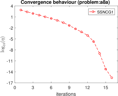
(a) Convergence behaviour (problem:a8a).

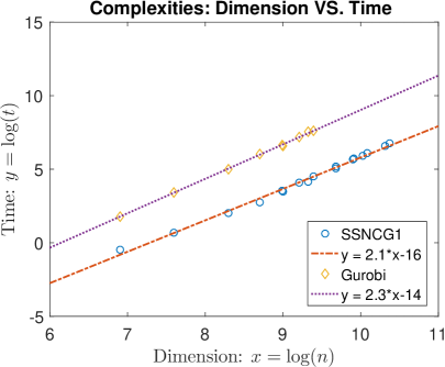
(b) Complexities: Dimension VS. Time.

Figure 1: Performance evaluations of Ssncg1.

In Table LABEL:table:projBPHPC, we report the detailed results obtained by our algorithm Ssncg1 and a recently developed algorithm (called PPROJ) in [18]. PPROJ is an extremely fast implementation of an algorithm which utilizes the sparse reconstruction by separable approximation [44] and the dual active set algorithm (DASA). We used the code downloaded from the authors’ homepage. Since PPROJ is implemented in C and it depends on some C libraries for linear system solvers, we have to compile PPROJ under the Linux system. Therefore, we compare the performance of Ssncg1 and PPROJ on the high performance computing (HPC) cluster at the National University of Singapore. Due to the memory limit imposed for each user, we are only able to test instances with the matrix dimensions less than 21,000. Default parameter values for PPROJ are used during the experiments. Note that since the stopping criterion of PPROJ is slightly different from ours, we report the accuracy measure $\eta$ corresponding to the solutions obtained by PPROJ. One can observe that, except the instance mushrooms, PPROJ can obtain highly accurate solutions. In fact, we observe from the detailed output file of PPROJ that it does not solve the instance mushrooms to the required accuracy while spending excessive amount of time on the DASA in computing Cholesky factorizations. One can also observe from Table LABEL:table:projBPHPC that Ssncg1 is much faster than PPROJ, especially for large scale problems. For example, for the instance rcv1, Ssncg1 is at least 52 times faster than PPROJ. Therefore, one can safely conclude that Ssncg1 is robust and highly efficient for solving projections problems over the Birkhoff polytope. However, we should emphasize here that PPROJ is a solver aiming at computing the projection onto a general polyhedral convex set and does not necessarily fully exploit the specific structure of the Birkhoff polytope. In fact, it would be an interesting future research topic to investigate whether PPROJ can take advantage of both the sparsity of the constraint matrix $B$ and the second order sparsity of the underlying problem to further accelerate its performance.

5.2 Numerical results for quadratic programming problems arising from relaxations of QAP problems

Given matrices $A,B\in{\cal S}^{n}$, the quadratic assignment problem (QAP) is given by

$$\min\{\langle X,\,AXB\rangle\mid X\in\{0,1\}^{n\times n}\cap\mathfrak{B}_{n}\},$$

where $\{0,1\}^{n\times n}$ denotes the set of matrices with only $0$ or $1$ entries. It has been shown in [1] that a reasonably good lower bound for the above QAP can often be obtained by solving the following convex QP problem:

$$\min\{\langle X,\,{\cal Q}X\rangle\mid X\in\mathfrak{B}_{n}\},$$ (32)

where the self-adjoint positive semidefinite linear operator ${\cal Q}$ is defined by

$${\cal Q}(X):=AXB-SX-XT,\quad\forall X\in\Re^{n\times n},$$

and $S,T\in{\cal S}^{n}$ are given as follows. Consider the eigenvalue decompositions, $A=V_{A}D_{A}V_{A}^{T}$, $B=V_{B}D_{B}V_{B}^{T}$, where $V_{A}$ and $D_{A}={\rm diag}{(\alpha_{1},\dots,\alpha_{n})}$ correspond to the eigenvectors and eigenvalues of $A$, and $V_{B}$ and $D_{B}={\rm diag}{(\beta_{1},\dots,\beta_{n})}$ correspond to the eigenvectors and eigenvalues of $B$, respectively. We assume that $\alpha_{1}\geq\ldots\geq\alpha_{n}$ and $\beta_{1}\leq\ldots\leq\beta_{n}$. Let $(\bar{s},\bar{t})$ be an optimal solution to the LP: $\max\{e^{T}s+e^{T}t\mid s_{i}+t_{j}\leq\alpha_{i}\beta_{j},\;i,j=1,\dots,n\}$, whose solution can be computed analytically as shown in [1]. Then $S=V_{A}{\rm diag}{(\bar{s})}V_{A}^{T}$ and $T=V_{B}{\rm diag}{(\bar{t})}V_{B}^{T}$. In our numerical experiments, the test instances $A$ and $B$ are obtained from the QAP Library [5]. We measure the accuracy of an approximate optimal solution $X$ for problem (32) by using the following relative KKT residual:

$$\eta=\frac{\|X-\Pi_{\mathfrak{B}_{n}}(X-{\cal Q}X)\|}{1+\|X\|+\|{\cal Q}X\|}.$$

Table LABEL:table:QAP reports the performance of the ALM designed in Section 4 against Gurobi in solving the QP (32). In the fourth and fifth columns of Table LABEL:table:QAP, “alm (itersub)” denotes the number of outer iterations with itersub in the parenthesis indicating the number of inner iterations of ALM. One can observe from Table LABEL:table:QAP that our algorithm is much faster than Gurobi, especially for large scale problems. For example, for the instance tai150b, ALM only needs 13 seconds to reach the desired accuracy while Gurobi needs about two and half hours. One can easily see that Algorithm ALM is highly efficient because each of its subproblems can be solved by the powerful semismooth Newton-CG algorithm Ssncg2 based on the efficient computations of $\Pi_{\mathfrak{B}_{n}}$ and its corresponding HS-Jacobian. Note that problem (32) is in fact a quadratic programming with $n^{2}$ variables. It is thus not surprising that the interior-point method based solver Gurobi reports out of memory for problem tai265c with $n=256$.

6 Conclusion

In this paper, we study the generalized Jacobians in the sense of Han and Sun [17] of the Euclidean projector over a polyhedral convex set with an emphasis on the Birkhoff polytope. A special element in the set of the generalized Jacobians, referred as the HS-Jacobian, is successfully constructed. Armed with its simple and explicit formula, we are able to provide a highly efficient procedure to compute the HS-Jacobian. To ensure the efficiency of our procedure, a dual inexact semismooth Newton method is designed and implemented to find the projection over the Birkhoff polytope. Numerical comparisons between the state-of-the-art solvers Gurobi and PPROJ have convincingly demonstrated the remarkable efficiency and robustness of our algorithm and implementation. To further demonstrate the importance of the fast computations of the projector and its corresponding HS-Jacobian, we also incorporate them in the augmented Lagrangian method for solving a class of Birkhoff polytope constrained convex QP problems. Extensive numerical experiments on a collection of QP problems arising from the relaxation of quadratic assignment problems show the large benefits of our second order nonsmooth analysis based procedure.

Table 3: The performance of ALM and Gurobi on the quadratic programming problems (32). In the table, “gu” stands for Gurobi; “alm” stands for ALM (accuracy $\eta<10^{-7}$). The entry “*” indicates out of memory. The computation time is in the format of “hours:minutes:seconds”. “00” in the time column means less than 0.5 seconds.

		iter	$\eta$	time
problem	$n$	gu $|$ alm (itersub)	gu $|$ alm	gu $|$ alm
lipa50a	50	11 $|$ 21 (58)	1.8-6 $|$ 7.3-8	11 $|$ 01
lipa50b	50	11 $|$ 17 (123)	2.2-6 $|$ 5.0-8	11 $|$ 05
lipa60a	60	11 $|$ 19 (54)	1.4-6 $|$ 6.7-8	30 $|$ 01
lipa60b	60	11 $|$ 18 (104)	1.7-6 $|$ 9.9-8	29 $|$ 05
lipa70a	70	11 $|$ 19 (52)	1.7-6 $|$ 6.0-8	1:17 $|$ 01
lipa70b	70	11 $|$ 19 (103)	1.4-6 $|$ 6.0-8	1:20 $|$ 06
lipa80a	80	11 $|$ 25 (68)	1.3-6 $|$ 7.3-8	2:46 $|$ 01
lipa80b	80	12 $|$ 18 (141)	6.3-7 $|$ 9.3-8	2:52 $|$ 14
lipa90a	90	11 $|$ 20 (54)	2.7-6 $|$ 8.8-8	5:32 $|$ 01
lipa90b	90	12 $|$ 19 (134)	5.5-7 $|$ 2.5-8	5:46 $|$ 15
sko100a	100	14 $|$ 26 (95)	8.5-6 $|$ 8.5-8	2:06 $|$ 11
sko100b	100	14 $|$ 27 (93)	8.3-6 $|$ 7.9-8	2:06 $|$ 10
sko100c	100	15 $|$ 27 (93)	4.5-6 $|$ 9.0-8	2:11 $|$ 11
sko100d	100	15 $|$ 26 (91)	4.8-6 $|$ 8.8-8	2:06 $|$ 10
sko100e	100	14 $|$ 27 (98)	5.8-6 $|$ 8.5-8	2:06 $|$ 11
sko100f	100	16 $|$ 27 (93)	6.1-6 $|$ 9.6-8	2:15 $|$ 09
sko64	64	13 $|$ 27 (91)	7.3-6 $|$ 9.0-8	13 $|$ 04
sko72	72	13 $|$ 26 (86)	8.1-6 $|$ 7.6-8	22 $|$ 04
sko81	81	14 $|$ 26 (89)	4.4-6 $|$ 7.6-8	43 $|$ 06
sko90	90	14 $|$ 26 (95)	4.4-6 $|$ 7.8-8	43 $|$ 08
tai100a	100	11 $|$ 18 (52)	1.3-6 $|$ 9.5-8	10:31 $|$ 02
tai100b	100	11 $|$ 27 (98)	1.3-6 $|$ 9.1-8	10:31 $|$ 13
tai50a	50	11 $|$ 20 (55)	1.1-6 $|$ 6.1-8	09 $|$ 01
tai50b	50	13 $|$ 25 (89)	5.9-6 $|$ 8.5-8	10 $|$ 03
tai60a	60	10 $|$ 19 (54)	5.4-6 $|$ 9.6-8	27 $|$ 01
tai60b	60	10 $|$ 28 (102)	5.4-6 $|$ 6.6-8	27 $|$ 06
tai80a	80	11 $|$ 21 (59)	1.2-6 $|$ 7.9-8	2:36 $|$ 01
tai80b	80	11 $|$ 27 (98)	1.2-6 $|$ 8.5-8	2:36 $|$ 07
tai256c	256	* $|$ 2 ( 4)	* $|$ 2.1-16	* $|$ 00
tai150b	150	19 $|$ 27 (94)	4.3-7 $|$ 9.3-8	2:46:17 $|$ 13
tho150	150	16 $|$ 24 (96)	5.6-6 $|$ 9.9-8	18:52 $|$ 22
wil100	100	13 $|$ 25 (82)	9.1-6 $|$ 8.8-8	2:14 $|$ 07
wil50	50	13 $|$ 29 (99)	3.9-6 $|$ 8.4-8	05 $|$ 03
esc128	128	17 $|$ 2 ( 4)	8.2-11 $|$ 2.2-16	09 $|$ 00

References

- [1] K. M. Anstreicher and N. W. Brixius, A new bound for the quadratic assignment problem based on convex quadratic programming, Mathematical Programming, 89 (2001), pp. 341–357.
- [2] A. Beck and M. Teboulle, A fast iterative shrinkage-thresholding algorithm for linear inverse problems, SIAM Journal on Imaging Sciences, 2 (2009), pp. 183–202.
- [3] G. Birkhoff, Three observations on linear algebra, Universidad Nacional de Tucumán, Revista, Serie A, 5 (1946), pp. 147–151.
- [4] J. F. Bonnans and A. Shapiro, Perturbation Analysis of Optimization Problems, Springer, New York, 2000.
- [5] R. E. Burkard, S. E. Karisch, and F. Rendl, QAPLIB — a quadratic assignment problem library, Journal of Global Optimization, 10 (1997), pp. 391–403.
- [6] C.-C. Chang and C.-J. Lin, LIBSVM: A library for support vector machines, ACM Transactions on Intelligent Systems and Technology, 2 (2011), pp. 27:1–27:27.
- [7] A. Chiche and J.Ch. Gilbert, How the augmented Lagrangian algorithm can deal with an infeasible convex quadratic optimization problem, Journal of Convex Analysis, 23 (2016), pp. 425–459.
- [8] F. H. Clarke, Optimization and Nonsmooth Analysis, John Wiley and Sons, New York, 1983.
- [9] Y. Cui, D. F. Sun, and K.-C. Toh, On the asymptotic superlinear convergence of the augmented Lagrangian method for semidefinite programming with multiple solutions, arXiv:1610.00875, 2016.
- [10] F. Delbos and J. Ch. Gilbert, Global linear convergence of an augmented Lagrangian algorithm to solve convex quadratic optimization problems, Journal of Convex Analysis, 12 (2005), pp. 45–69.
- [11] R. L. Dykstra, An algorithm for restricted least squares regression, Journal of the American Statistical Association, 78 (1983), pp. 837-842.
- [12] A. Fischer and C. Kanzow, On finite termination of an iterative method for linear complementarity problems, Mathematical Programming, 74 (1996), pp. 279–292.
- [13] F. Fogel, R. Jenatton, F. Bach, and A. d’Aspremont, Convex relaxations for permutation problems, Advances in Neural Information Processing Systems, 2013, pp. 1016–1024.
- [14] D. Gabay and B. Mercier, A dual algorithm for the solution of nonlinear variational problems via finite element approximations, Computers & Mathematics with Applications, 2 (1976), pp. 17–40.
- [15] R. Glowinski and A. Marroco, Sur l’approximation, par elements finis d’ordre un, et la resolution, par penalisation-dualit’e, d’une classe de problemes de Dirichlet non lineares, Revue Francaise d’Automatique, Informatique et Recherche Op’erationelle, 9 (R-2) (1975), pp. 41–76.
- [16] I. Gurobi Optimization, Gurobi Optimizer Reference Manual, 2016.
- [17] J. Y. Han and D. F. Sun, Newton and quasi-Newton methods for normal maps with polyhedral sets, Journal of Optimization Theory and Applications, 94 (1997), pp. 659–676.
- [18] W. W. Hager and H. Zhang, Projection onto a polyhedron that exploits sparsity, SIAM Journal on Optimization, 26 (2016), pp. 1773–1798.
- [19] N. Higham, Computing the nearest symmetric correlation matrix–a problem from finance, IMA Journal of Numerical Analysis, 22 (2002), pp. 329–343.
- [20] A. Haraux, How to differentiate the projection on a convex set in Hilbert space. Some applications to variational inequalities, Journal of the Mathematical Society of Japan, 29 (1977), pp. 615–631.
- [21] J.-B. Hiriart-Urruty, J.-J. Strodiot, and V. H. Nguyen, Generalized Hessian matrix and second-order optimality conditions for problems with data, Applied Mathematics and Optimization, 11 (1984), pp. 43–56.
- [22] B. Jiang, Y. F. Liu, and Z. W. Wen, -norm regularization algorithms for optimization over permutation matrices, SIAM Journal on Optimization, 26 (2016), pp. 2284–2313.
- [23] X. D. Li, D. F. Sun, and K.-C. Toh, QSDPNAL: A two-phase augmented Lagrangian method for convex quadratic semidefinite programming, Mathematical Programming Computation, in print, 2018.
- [24] X. D. Li, D. F. Sun, and K.-C. Toh, A highly efficient semismooth Newton augmented Lagrangian method for solving Lasso problems, SIAM Journal on Optimization, 28 (2018), pp. 433–458.
- [25] C. H. Lim and S. J. Wright, Beyond the Birkhoff polytope: convex relaxations for vector permutation problems, Advances in Neural Information Processing Systems, 2014, pp. 2168–2176.
- [26] J. Malick, A dual approach to semidefinite least-squares problems, SIAM Journal on Matrix Analysis and Applications, 26 (2004), pp. 272–284.
- [27] F. J. Luque, Asymptotic convergence analysis of the proximal point algorithm, SIAM Journal on Control and Optimization, 22 (1984), pp. 277–293.
- [28] R. Mifflin, Semismooth and semiconvex functions in constrained optimization, SIAM Journal on Control and Optimization, 15 (1977), pp. 959–972.
- [29] Y. Nesterov, A method of solving a convex programming problem with convergence rate , Soviet Mathematics Doklady, 27 (1983), pp. 372–376.
- [30] J.-S. Pang, Newton’s method for B-differentiable equations, Mathematics of Operations Research, 15 (1990), pp. 311–341.
- [31] J.-S. Pang and D. Ralph, Piecewise smoothness, local invertibility, and parametric analysis of normal maps, Mathematics of Operations Research, 21 (1996), pp. 401–426.
- [32] H. Qi and D. F. Sun, A quadratically convergent Newton method for computing the nearest correlation matrix, SIAM Journal on Matrix Analysis and Applications, 28 (2006), pp. 360–385.
- [33] L. Qi and J. Sun, A nonsmooth version of Newton’s method, Mathematical Programming, 58 (1993), pp. 353–367.
- [34] S. M. Robinson, Some continuity properties of polyhedral multifunctions, in Mathematical Programming at Oberwolfach, vol. 14 of Mathematical Programming Studies, Springer Berlin Heidelberg, 1981, pp. 206–214.
- [35] S. M. Robinson, Implicit B-differentiability in generalized equations, Technical report #2854, Mathematics Research Center, University of Wisconsin, Madison (1985).
- [36] R. T. Rockafellar, Convex Analysis, Princeton University Press, Princeton, N.J., 1970.
- [37] R. T. Rockafellar, Augmented Lagrangians and applications of the proximal point algorithm in convex programming, Mathematics of Operations Research, 1 (1976), pp. 97–116.
- [38] R. T. Rockafellar and R. J.-B. Wets, Variational Analysis, Springer, New York, 1998.
- [39] D. F. Sun, J. Y. Han, and Y. Zhao, On the finite termination of the damped-Newton algorithm for the linear complementarity problem, Acta Mathematica Applicatae Sinica, 21 (1998), pp. 148–154.
- [40] J. Sun, On Monotropic Piecewise Quadratic Programming, PhD thesis, Department of Mathematics, University of Washington, 1986.
- [41] L. N. Trefethen and D. Bau III, Numerical Linear Algebra, SIAM, Philadelphia, 1997.
- [42] J. Von Neumann, A certain zero-sum two-person game equivalent to an optimal assignment problem, Annals of Mathematical Studies, 28 (1953), pp. 5–12.
- [43] F. Wang, P. Li, and A. C. Konig, Learning a bi-stochastic data similarity matrix, 2010 IEEE 10th International Conference on Data Mining (ICDM), pp. 551–560.
- [44] S. J. Wright, R. D. Nowak, and M. A. T. Figueiredo, Sparse reconstruction by separable approximation, IEEE Transactions on Signal Processing, 57 (2009), pp. 2479–2493.
- [45] X. Zhao, D. F. Sun, and K.-C. Toh, A Newton-CG augmented Lagrangian method for semidefinite programming, SIAM Journal on Optimization, 20 (2010), pp. 1737–1765.