On a variable step size modification of Hines’ method in computational neuroscience

Abstract

For simulating large networks of neurons Hines proposed a method which uses extensively the structure of the arising systems of ordinary differential equations in order to obtain an efficient implementation. The original method requires constant step sizes and produces the solution on a staggered grid. In the present paper a one-step modification of this method is introduced and analyzed with respect to their stability properties. The new method allows for step size control. Local error estimators are constructed. The method has been implemented in matlab and tested using simple Hodgkin-Huxley type models. Comparisons with standard state-of-the-art solvers are provided.

Keywords: partitioned midpoint rule, stability of splitting methods, Hodkin-Huxley models, networks of neurons

Classification: AMS MSC (2010) 65L20, 65L05, 65L06, 92C42

KTH Royal Institute of Technology, Department of Mathematics, 100 44 Stockholm, Sweden

1 Introduction

When simulating large networks of neurons a considerable part of the model consists of the electrical subsystem which in turn extensively uses the classical Hodkin-Huxley model of nerve activity. Owing to the large size of the networks to be modeled the efficient numerical solution of the arising high-dimensional system of ordinary differential equations is of extraordinary importance. Complex program systems, e.g., NEURON [4], GENESIS [2], and many others are in routine use in order to solve them. In order to construct efficient numerical methods it is necessary to tailor the methods to the special properties of the system. The building block is often (variants of) the Hodgkin-Huxley system [9]

$$C\frac{dV}{dt} =I(t)-g_{K}n^{4}(V-V_{K})-g_{Na}m^{3}h(V-V_{Na})-g_{L}(V-V_{L}),$$ (1)

$$\frac{dn}{dt} =\alpha_{n}(V)(1-n)-\beta_{n}(V)n,$$ (2)

$$\frac{dm}{dt} =\alpha_{m}(V)(1-m)-\beta_{m}(V)m,$$ (3)

$$\frac{dh}{dt} =\alpha_{h}(V)(1-h)-\beta_{h}(V)h.$$ (4)

The coefficients $\alpha_{i}(V)$ and $\beta_{i}(V)$ are highly nonlinear functions of their argument. The key observation in this system is that the differential equation for the voltage $V$ is linear in $V$ while the differential equations for the gate variables $n,m,h$ are linear in those. Slightly more general, this system has the structure

$$x^{\prime} =A(y)x+b(y,t),$$ (5)

$$y^{\prime} =c(x,t)+D(x)y.$$ (6)

Here, $x$ denotes the voltage while $y$ is the vector of gate variables, or vice versa. In general, this model leads to stiff differential equations such that implicit time stepping methods are necessary. Standard approaches require the solution of a nonlinear system of equations in every step by using variants of Newton’s method. Given the large dimension of the usual models, this property may become a severe restriction. Hines [8] came up with the idea to discretize the system in two steps: First, the differential equation for $x$ is discretized leading to a linear system to be solved. Then, the differential equation for $y$ is discretized. Also here it remains only a linear system to be solved in contrast to a fully nonlinear system in the standard approach. Note that the lower dimensional systems have often a very special structure such that they can be solved very efficiently. In particular, for the Hodgkin-Huxley system (1) – (4), both systems have a diagonal system matrix.

Hines chose the implicit midpoint rule as the basic discretization. The discrete approximations of $x$ and $y$ are defined on a staggered grid. In order to fix notation, let $t\in[0,T]$ for some $T>0$ and $h>0$ be a given step size. For $n=0,1,2,\ldots$ let

$$t_{n}=nh,\quad t_{n+1/2}=(n+1/2)h.$$

Hines method reads

$$x_{n+1} =x_{n}+h\left(A(y_{n+1/2})\frac{x_{n+1}+x_{n}}{2}+b(y_{n+1/2},t)\right),$$ (7)

$$y_{n+3/2} =y_{n+1/2}+h\left(c(x_{n+1},t_{n+1})+D(x_{n+1})\frac{y_{n+3/2}+y_{n+1/2}}{2}\right).$$ (8)

This method has the following properties:

• The approximations are available on a staggered grid, only: $x_{n}\approx x(t_{n})$ and $y_{n+1/2}\approx y(t_{n+1/2})$.

• Since initial values are available for $t=0$ only, the first approximation $y_{1/2}$ must be computed by other means.

• The method is second order accurate. However, this property is only preserved if the step size is constant.

In particular the last property calls for a modification of this method such that a step size control becomes possible.

In this paper, we consider the following modification of Hines’ method:

$$x_{n+1/2} =x_{n}+\frac{h}{2}A(y_{n})x_{n}+b(y_{n},t_{n}),$$ (9)

$$y_{n+1} =y_{n}+h\left(c(x_{n+1/2},t_{n+1/2})+D(x_{n+1/2})\frac{y_{n+1}+y_{n}}{2}\right),$$ (10)

$$x_{n+1} =x_{n+1/2}+\frac{h}{2}(A(y_{n+1})x_{n+1}+b(y_{n+1},t_{n+1})).$$ (11)

Since the first of these three equation is an explicit Euler step, the computational work of the latter method is only slightly more expensive than that of the original proposal by Hines. However, the modified version is a genuine one-step method allowing for a step size change without sacrificing the order.

In this note we will investigate the numerical properties of this method. In particular, we are interested in the asymptotic stability of this method. Moreover, we will propose an efficient implementation. In the final section a few numerical examples will be provided.

2 Properties of the method

In order to simplify the notation slightly, we consider the system

$$x^{\prime} =f(x,y,t),$$ (12)

$$y^{\prime} =g(x,y,t).$$ (13)

The method (9) – (11) reduces to

$$x_{n+1/2} =x_{n}+\frac{h}{2}f(x_{n},y_{n},t_{n}),$$ (14)

$$y_{n+1} =y_{n}+hg(x_{n+1/2},\frac{1}{2}(y_{n+1}+y_{n}),t_{n+1/2}),$$ (15)

$$x_{n+1} =x_{n+1/2}+\frac{h}{2}f(x_{n+1},y_{n+1},t_{n+1}).$$ (16)

By eliminating the intermediate approximation $x_{n+1/2}$, this system reduces to

$$x_{n+1} =x_{n}+\frac{h}{2}(f(x_{n+1},y_{n+1},t_{n+1})+f(x_{n},y_{n},t_{n})),$$ (17)

$$y_{n+1} =y_{n}+hg(x_{n}+\frac{h}{2}f(x_{n},y_{n},t_{n}),\frac{1}{2}(y_{n+1}+y_{n}),t_{n+1/2}).$$ (18)

Let $(x^{\ast},y^{\ast})$ denote the solution of (12) – (13) on $[0,T]$ subject to the initial condition $x(0)=x_{0}$ and $y(0)=y_{0}$. Uniqueness is guaranteed if $f$ and $g$ are Lipschitz continuous with respect to $x$ and $y$ and continuous with respect to $t$ in a neighborhood $U$ of the trajectory $\Gamma=\{(x^{\ast}(t),y^{\ast}(t),t)|t\in[0,T]\}$.

Define, for sequences $\{(x_{n},y_{n})\}_{n=0}^{N(h)}$, the discretization error by

$${\cal N}_{x}(x_{n},y_{n}) =\frac{x_{n+1}-x_{n}}{h}-\frac{1}{2}(f(x_{n}y_{n}t_{n})+f(x_{n+1},y_{n+1},t_{n+1})),$$

$${\cal N}_{y}(x_{n},y_{n}) =\frac{y_{n+1}-y_{n}}{h}-g(x_{n}+\frac{h}{2}f(x_{n},y_{n},t_{n}),\frac{1}{2}(y_{n+1}+y_{n}),t_{n+1/2}).$$

The method is called stable if there exist an $h_{0}$ and a $K$ such that, for $h<h_{0}$ and for any sequences $\{(x_{n}^{j},y_{n}^{j})\}_{n=0}^{N(h)}$, $j=1,2$ belonging to $U$ it holds

$$\max_{n=0,\ldots N(h)}(|x_{n}^{1}-x_{n}^{2}|+|y_{n}^{1}-y_{n}^{2}|)\leq K\left\{|x_{0}^{1}-x_{0}^{2}|+|y_{0}^{1}-y_{0}^{2}|+\right.\\ \left.\max_{n=0,\ldots,N(h)}\left(|{\cal N}_{x}(x_{n}^{1},y_{n}^{1})-{\cal N}_{x}(x_{n}^{2},y_{n}^{2})|+|{\cal N}_{y}(x_{n}^{1},y_{n}^{1})-{\cal N}_{y}(x_{n}^{2},y_{n}^{2})|\right)\right\}.$$

This definition follows [1, Section 5.2.3].

Proposition 1.

Let $(x^{\ast},y^{\ast})$ be solutions of (12) – (13) on $[0,T]$ subject to the initial condition $x(0)=x_{0}$ and $y(0)=y_{0}$. Let $f$ and $g$ be Lipschitz continuous with respect to $x$ and $y$ and continuous with respect to $t$ in a neighborhood $U$ of the trajectory $\Gamma=\{(x^{\ast}(t),y^{\ast}(t),t)|t\in[0,T]\}$. Then, the method (14) – (16) is stable.

Proof.

The method is a combination of two implicit Runge-Kutta methods. So the proof is standard. ∎

Proposition 2.

Let the assumptions of Theorem 1 be fulfilled and $f$ and $g$ be sufficiently often differentiable. Then, (14) – (16) is a second order method and the global error has an asymptotic expansion in powers of $h^{2}$.

Proof.

As a Runge-Kutta method, the local error possesses an expansion in powers of $h$, [5, Theorem 3.2]. Taylor expansion shows that, for the truncation error, it holds

$${\cal N}_{x}(x^{\ast}(t_{n}),y^{\ast}(t_{n}))=O(h^{2}),\quad{\cal N}_{y}(x^{\ast}(t_{n}),y^{\ast}(t_{n}))=O(h^{2}).$$

Since the method is stable, it is second order convergent.

Rewriting (17), it holds $x_{n}+(h/2)f(x_{n},y_{n},t_{n})=x_{n+1}-(h/2)f(x_{n+1},y_{n+1},t_{n+1})$ such that (18) can be rewritten as

$$y_{n}=y_{n+1}-hg(x_{n+1}-(h/2)f(x_{n+1},y_{n+1},t_{n+1}),\frac{1}{2}(y_{n+1}+y_{n}),t_{n+1/2}).$$

Hence, the method is symmetric and the assertion about the asymptotic expansion follows from [5, Theorem 8.10]. ∎

A more interesting question is the asymptotic properties of this method. Recall that the system to be solved is usually stiff. This is also the case if the two components are considered individually, that is (12) for fixed $y$ and (13) for fixed $x$. So the standard notions of asymptotic stability that base on the test scalar equation $z^{\prime}=\lambda z$ are not useful here. A more appropriate test equation must have at least two components. This leads to the proposal

$$x^{\prime} =\mu x+ay,$$ (19)

$$y^{\prime} =bx+\lambda y,$$ (20)

where

$$\mu,\lambda<0\text{ and }ab<\mu\lambda.$$ (21)

Under these conditions, the system is asymptotically stable as well as the individual components are. This test system has been proposed by Strehmel&Weiner [18] in order to characterize stability properties of partitioned Runge-Kutta methods.

The method (14) – (16) applied to (19) – (20) gives rise to

$$A\left(\begin{array}[]{c}x_{n+1}\\ y_{n+1}\end{array}\right)=B\left(\begin{array}[]{c}x_{n}\\ y_{n}\end{array}\right)$$ (22)

where

$$A =\left(\begin{array}[]{cc}1-\frac{h\mu}{2}&-\frac{ha}{2}\\ 0&1-\frac{h\lambda}{2}\end{array}\right),$$

$$B =\left(\begin{array}[]{cc}1+\frac{h\mu}{2}&\frac{ha}{2}\\ hb\left(1+\frac{h\mu}{2}\right)&1+\frac{h\lambda}{2}+\frac{abh^{2}}{2}\end{array}\right).$$

This recursion can be rewritten in the form

$$\left(\begin{array}[]{c}x_{n+1}\\ y_{n+1}\end{array}\right)=C\left(\begin{array}[]{c}x_{n}\\ y_{n}\end{array}\right)$$

with

$$C=\left(\begin{array}[]{cc}\alpha\left(1+\gamma\frac{h\mu}{2}(\beta-1)\right)&ha\left(\frac{1}{\left(1-\frac{h\mu}{2}\right)\left(1-\frac{h\lambda}{2}\right)}+\frac{\gamma}{4}(\alpha-1)(\beta-1)\right)\\ hb\frac{1+\frac{h\mu}{2}}{1-\frac{h\lambda}{2}}&\beta+\gamma(\beta-1)\frac{h\mu}{2}\end{array}\right)$$

where

$$\alpha=\frac{1+\frac{h\mu}{2}}{1-\frac{h\mu}{2}},\quad\beta=\frac{1+\frac{h\lambda}{2}}{1-\frac{h\lambda}{2}}$$

are the stability functions of the midpoint and trapezoidal rule, respectively, applied to the equations (19) – (20) individually. Note that, under the conditions (21), it holds $|\alpha|<1$ and $|\beta|<1$.

The recursion is asymptotically stable if and only if the eigenvalues of $C$ are less than one in absolute value. A short computation shows that the characteristic polynomial of $C$ has the form

$$\chi(s)=s^{2}-(\alpha+\beta+\gamma(\alpha-1)(\beta-1))s+\alpha\beta$$

were $\gamma=\frac{ab}{\mu\lambda}$.

Lemma 3.

Consider the polynomial $\chi(s)=s^{2}-(\alpha+\beta+\gamma(\alpha-1)(\beta-1))s+\alpha\beta$ with $|\alpha|<1$ and $|\beta|<1$. For the roots $s_{1}$ and $s_{2}$ of $\chi(s)=0$ it holds $\max(|s_{1}|,|s_{2}|)<1$ if and only if

$$-\frac{(1+\alpha)(1+\beta)}{(1-\alpha)(1-\beta)}<\gamma<1.$$

Remark.

Under the assumption (21) it holds $\gamma<1$. Note that $\gamma$ may be negative.

Proof.

We use the change of variables

$$w(z)=\frac{1+z}{1-z}.$$

$w$ maps the negative complex halfplane $\mathbb{C}^{-}=\{z\in\mathbb{C}|\mathfrak{R}z<0\}$ uniquely onto the disk $S=\{z\in\mathbb{C}||z|<1\}$. So it holds $s_{1},s_{2}\in S$ if and only if $z_{1},z_{2}\in\mathbb{C}^{-}$ for the zeros of $\chi(w(z))$. Denote for short $\chi(s)=s^{2}+a_{1}s+a_{0}$. A short calculation provides

$$\chi(w(z))=\frac{z^{2}(1-a_{1}+a_{0})+z(2-2a_{0})+(1+a_{1}+a_{0})}{(1-z)^{2}}.$$

The zeros of this functions are those of the enumerator polynomial $\eta(z)=c_{2}z^{2}+c_{1}z+c_{0}$ where

$$c_{2} =1+(\alpha+\beta+\gamma(\alpha-1)(\beta-1))+\alpha\beta,$$

$$c_{1} =2-2\alpha\beta,$$

$$c_{0} =1-(\alpha+\beta+\gamma(\alpha-1)(\beta-1))+\alpha\beta.$$

According to the Routh-Hurwitz criterion [5, Theorem I.13.4] the roots of $\eta$ lie all in $\mathbb{C}^{-}$ if and only if all coefficients $c_{i}$ have the same sign. Since $|\alpha\beta|<1$, it holds $c_{1}>0$. The condition $c_{0}>0$ is equivalent to

$$\frac{1+\alpha\beta-\alpha-\beta}{(\alpha-1)(\beta-1)}=1>\gamma$$

while $c_{2}>0$ is equivalent to

$$\frac{-(\alpha+1)(\beta+1)}{(\alpha-1)(\beta-1)}<\gamma.$$

This completes the proof. ∎

Theorem 4.

Under the assumption $\mu,\lambda<0$, the recursion (22) is asymptotically stable if and only if

$$-\frac{(1+\alpha)(1+\beta)}{(1-\alpha)(1-\beta)}<\gamma<1.$$

The assertion is a consequence of Lemma 3.

Corollary 5.

For every $\gamma<0$, there exists a $h(\mu,\lambda,\gamma)>0$ such that the recursion (22) is unstable for all $h>h(\mu,\lambda,\gamma)$.

Proof.

One can easily show that $\alpha=\alpha(h)$ and $\beta=\beta(h)$ are monotonically decreasing functions of $h$. Moreover,

$$\varphi(h)=\frac{1+\alpha}{1-\alpha}$$

is a monotonically decreasing function of $\alpha$ and it holds $\lim_{h\rightarrow 0}\varphi(\alpha(h))=\infty$ and $\lim_{h\rightarrow\infty}\varphi(\alpha(h))=0$. ∎

Remark.

It is interesting to see how the corresponding results for the original Hines’ method look like. The recursion becomes

$$\left(\begin{array}[]{c}x_{n+1}\\ y_{n+3/2}\end{array}\right)=C_{\textrm{Hines}}\left(\begin{array}[]{c}x_{n}\\ y_{n+1/2}\end{array}\right)$$

with

$$C_{\textrm{Hines}} =\left(\begin{array}[]{cc}\alpha&\frac{ha}{\left(1-\frac{h\mu}{2}\right)}\\ \alpha\frac{hb}{\left(1-\frac{h\lambda}{2}\right)}&\beta+\frac{abh^{2}}{\left(1-\frac{h\mu}{2}\right)\left(1-\frac{h\lambda}{2}\right)}\end{array}\right)$$

$$=\left(\begin{array}[]{cc}\alpha&\frac{ha}{\left(1-\frac{h\mu}{2}\right)}\\ \alpha\frac{hb}{\left(1-\frac{h\lambda}{2}\right)}&\beta+\gamma(1-\alpha)(1-\beta)\end{array}\right).$$

It holds

$$\textrm{trace}(C_{\textrm{Hines}}) =\alpha+\beta+\gamma(1-\alpha)(1-\beta),$$

$$\det(C_{\textrm{Hines}}) =\alpha\beta+\alpha\gamma(1-\alpha)(1-\beta)-\alpha\frac{abh^{2}}{\left(1-\frac{h\mu}{2}\right)\left(1-\frac{h\lambda}{2}\right)}$$

$$=\alpha\beta.$$

So the stability polynomial of Hines’ method and its modification (9) – (11) are identical.

3 The relation of this method to Strang’s splitting and the Peaceman-Rachford method

3.1 Strang’s splitting

In this section, we will consider an approach to solving (12) – (13) using a splitting method. For that, let

$$U=\left(\begin{array}[]{c}x\\ y\end{array}\right),\quad F(U,t)=\left(\begin{array}[]{c}f(x,y,t)\\ g(x,y,t)\end{array}\right).$$

Then (12) – (13) is equivalent to $U^{\prime}=F(U,t)$. Introduce the splitting

$$F(U,t)=F_{1}(U,t)+F_{2}(U,t)=\left(\begin{array}[]{c}f(x,y,t)\\ 0\end{array}\right)+\left(\begin{array}[]{c}0\\ g(x,y,t)\end{array}\right).$$ (23)

A classical example of operator splitting is Strang’s approach [17]. In order to advance the solution one step of step size $h$ from $t_{n}$ to $t_{n+1}$ the system $U^{\prime}=F_{1}(U,t)$ is first integrated over the interval $[t_{n},t_{n}+h/2]$, then the results are used to integrate the system $U^{\prime}=F_{2}(U,t)$ on $[t_{n},t_{n+1}]$, and finally the first system on $[t_{n+1}-h/2,t_{n+1}]$. For the decomposition (23), this gives rise to the following three steps:

1. Integrate $x^{\prime}=f(x,y_{n},t)$, $x(t_{n})=x_{n}$ on $[t_{n,}t_{n}+h/2]$. Denote $x_{n+1/2}=x(t_{n}+h/2)$.

2. Integrate $y^{\prime}=g(x_{n+1/2},y,t)$, $y(t_{n})=y_{n}$ on $[t_{n},t_{n+1}]$. Denote $y_{n+1}=y(t_{n+1})$.

3. Integrate $x^{\prime}=f(x,y_{n+1},t)$, $x(t_{n}+h/2)=x_{n+1/2}$ on $[t_{n+1}-h/2,t_{n+1}]$. Let $x_{n+1}=x(t_{n+1})$.

Even if $f,g$ are linear functions, the operators $F_{1}$ and $F_{2}$ do not commute. So we expect the splitting to be second order accurate at least in the linear case (e.g., [10, Chapter 4]). A comparison with the finite difference method (14) – (16) reveals that the latter can be interpreted as a second order discretization of Strang’s splitting.

Let us ask the question of asymptotic stability of Strang’s splitting applied to the test system (19) – (20). Similarly as before the recursion can be written down in the form

$$\left(\begin{array}[]{c}x_{n+1}\\ y_{n+1}\end{array}\right) =C_{\text{Strang}}\left(\begin{array}[]{c}x_{n}\\ y_{n}\end{array}\right)$$ (28)

$$C_{\text{Strang}} =\left(\begin{array}[]{cc}\alpha+\alpha^{1/2}T&\frac{a}{\mu}\left(\alpha^{1/2}-1\right)\left(\alpha^{1/2}+T+\beta\right)\\ \frac{b}{\lambda}\alpha^{1/2}\left(\beta-1\right)&T+\beta\end{array}\right)$$ (31)

where $T=\gamma\left(\alpha^{1/2}-1\right)\left(\beta-1\right)$. Here,

$$\alpha=e^{\mu h},\quad\beta=e^{\lambda h}.$$

The characteristic polynomial becomes

$$\chi(s)=s^{2}-(\alpha+\beta+\gamma(\alpha-1)(\beta-1))s+\alpha\beta.$$

This is structurally identical to the one for the discrete case.

Theorem 6.

Let $\mu<0$ and $\lambda<0$. The recursion (28) is asymptotically stable if and only if

$$-\frac{\left(1+e^{h\mu}\right)\left(1+e^{h\lambda}\right)}{\left(e^{h\mu}-1\right)\left(e^{h\lambda}-1\right)}<\gamma<1.$$

Proof.

The result is a consequence of the results of Lemma 3 by setting $\alpha=e^{h\mu}$ and $\beta=e^{h\lambda}$. ∎

Note that always $\gamma<1$ under the assumption $ab<\mu\lambda$. Moreover, for any $h>0,\mu<0,\lambda<0$ and

$$\psi(h)=\frac{\left(1+e^{h\mu}\right)\left(1+e^{h\lambda}\right)}{\left(e^{h\mu}-1\right)\left(e^{h\lambda}-1\right)}$$

it holds that $\psi$ is a monotonically decreasing function with $\lim_{h\rightarrow 0}\psi(h)=\infty$ and $\lim_{h\rightarrow\infty}\psi(h)=1$. We have immediately

Corollary 7.

If $\gamma<-1$ and $\mu<0,\lambda<0$, the there exist always an $h(\gamma,\mu,\lambda)>0$ such that the recursion (28) is unstable for $h>h(\gamma,\mu,\lambda)$.

Compared to the discrete case, the stability domain is slightly larger for Strang’s splitting. However, even here the stability domain is bounded.

3.2 The Peaceman-Rachford method

The Peaceman-Rachford method was introduced in [13] in order to solve semidiscretized linear parabolic partial differential equations. If the system (12) – (13) is splitted according to (23), the solution $U$ is then advanced from $t_{n}$ to $t_{n+1}$ by

$$U_{n+1/2} =U_{n}+\frac{h}{2}\left(F_{1}(U_{n+1/2},t_{n+1/2})+F_{2}(U_{n},t_{n})\right),$$

$$U_{n+1} =U_{n+1/2}+\frac{h}{2}\left(F_{1}(U_{n+1/2},t_{n+1/2})+F_{2}(U_{n+1},t_{n+1})\right).$$

The application of the Peaceman-Rachford method in (23) leads to

$$\left(\begin{array}[]{c}x_{n+1/2}\\ y_{n+1/2}\end{array}\right) =\left(\begin{array}[]{c}x_{n}\\ y_{n}\end{array}\right)+\frac{h}{2}\left(\left(\begin{array}[]{c}0\\ g(x_{n+1/2},y_{n+1/2},t_{n+1/2}\end{array}\right)+\left(\begin{array}[]{c}f(x_{n},y_{n},t_{n})\\ 0\end{array}\right)\right),$$

$$\left(\begin{array}[]{c}x_{n+1}\\ y_{n+1}\end{array}\right) =\left(\begin{array}[]{c}x_{n+1/2}\\ y_{n+1/2}\end{array}\right)+\frac{h}{2}\left(\left(\begin{array}[]{c}0\\ g(x_{n+1/2},y_{n+1/2},t_{n+1/2}\end{array}\right)+\left(\begin{array}[]{c}f(x_{n+1},y_{n+1},t_{n+1})\\ 0\end{array}\right)\right).$$

Writing out the components, this recursion becomes

(i)

$x_{n+1/2}=x_{n}+\frac{h}{2}f(x_{n},y_{n},t_{n})$

(ii)

$y_{n+1/2}=y_{n}+\frac{h}{2}g(x_{n+1/2},y_{n+1/2},t_{n+1/2})$

(iii)

$y_{n+1}=y_{n+1/2}+\frac{h}{2}g(x_{n+1/2},y_{n+1/2},t_{n+1/2})$

(iv)

$x_{n+1}=x_{n+1/2}+\frac{h}{2}f(x_{n+1},y_{n+1},t_{n+1})$

Inserting (i) into (iv) we obtain

$$x_{n+1}=x_{n}+\frac{h}{2}\left(f(x_{n},y_{n},t_{n})+f(x_{n+1},y_{n+1},t_{n+1})\right).$$

Similarly, from (ii) and (iii) we have

$$y_{n+1}=y_{n}+hg(x_{n}+\frac{h}{2}f(x_{n},y_{n},t_{n}),y_{n+1/2},t_{n+1/2}).$$

By subtracting (ii) and (iii) we arrive at

$$y_{n+1/2}=\frac{1}{2}\left(y_{n}+y_{n+1}\right).$$

Hence, the Peaceman-Rachford method applied to our system becomes

$$x_{n+1} =x_{n}+\frac{h}{2}\left(f(x_{n},y_{n},t_{n})+f(x_{n+1},y_{n+1},t_{n+1})\right),$$

$$y_{n+1} =y_{n}+hg(x_{n}+\frac{h}{2}f(x_{n},y_{n},t_{n}),\frac{1}{2}\left(y_{n}+y_{n+1}\right),t_{n+1/2}).$$

So this method is equivalent to (17) – (18).

The Peaceman-Rachford method has been used extensively to solve partial differential equations. There, one is mainly interested in showing stability properties independent of the spatial discretization. These stability estimates are often based on monotonicity assumptions (one-sided Lipschitz conditions) on the right-hand side $F_{1},F_{2}$. In particular, let the condition

$$\left\langle F_{i}(\tilde{w},t)-F_{i}(w,t),\tilde{w}-w\right\rangle\leq\nu\|\tilde{w}-w\|^{2},\quad i=1,2,$$

hold for all $\tilde{w},w$ and $t$ with a certain constant $\nu\in\mathbb{R}$. Here, $\left\langle\cdot\right\rangle$ denotes the Euclidean inner product and $\|\cdot\|$ the Euclidean norm. Hundsdorfer&Verwer [11] show that the method is unconditionally stable (that is, for all step sizes $h$) if $\nu\leq 0$. However, if $\nu>0$, stability can only be guaranteed if the step size is restricted by $h\nu<2$.

How do these results translate to our model system

$$x^{\prime} =\mu x+ay,$$

$$y^{\prime} =bx+\lambda y,$$

where $\mu,\lambda<0$ and $ab<\mu\lambda$?

In the linear autonomous case, the monotonicity requirement reduces to

$$w^{T}F_{i}(w)\leq\nu\|w\|^{2}\quad\text{for all }w.$$

We have

$$w^{T}F_{2}(w)\leq\nu\|w\|^{2}\text{ for all }w \Longleftrightarrow y(bx+\lambda y)\leq\nu(x^{2}+y^{2})\text{ for all }x,y$$

$$\Longleftrightarrow 0\leq\nu x^{2}-bxy+(\nu-\lambda)y^{2}\text{ for all }x,y.$$

For the latter inequality to hold for all $x,y$, we must have $\nu\geq 0$.

$$w^{T}F_{2}(w)\leq\nu\|w\|^{2}\text{ for all }w \Longleftrightarrow 0\leq\left(\sqrt{\nu}x-\frac{1}{2\sqrt{\nu}}by\right)^{2}+\left(\nu-\lambda-\frac{b^{2}}{4\nu}\right)y^{2}\text{ for all }x,y$$

$$\Longleftrightarrow 0\leq\nu-\lambda-\frac{b^{2}}{4\nu}$$

$$\Longleftrightarrow\frac{1}{2}(\lambda+\sqrt{\lambda^{2}+b^{2}})\leq\nu.$$

Similarly,

$$w^{T}F_{1}(w)\leq\nu\|w\|^{2}\text{ for all }w\Longleftrightarrow\frac{1}{2}(\mu+\sqrt{\mu^{2}+a^{2}})\leq\nu.$$

Hence, we have always $\nu>0$ unless $a=b=0$.

4 Implementation

For an efficient implementation, estimations of the local error and step size control are of utmost importance. In this section we will discuss these issues.

The method (14) – (16) does not have an imbedded error estimator. So we have two possibilities for estimating the local error:

1. Since the discrete solution possesses an asymptotic expansion in powers of $h^{2}$, the error can be estimated via Richardson extrapolation. This can be combined with local extrapolation.

2. Use the detailed representation of the leading error term.

The first idea seems to be rather straightforward. However, one has to keep in mind that the individual equations in (5) – (6) are often stiff, and the discretization reduces to the trapezoidal rule and the implicit midpoint rule, respectively, for decoupled systems. For such systems and these discretizations, we expect a simple step size halving to behave very badly when using local extrapolation since the resulting method has a bounded stability domain [6, p. 133]. In fact, when applying our method and step size halving to Hodkin-Huxley systems, we observed a behavior of the method which is typical for instabilities due to too large step sizes at low tolerances. Therefore, we implemented two versions:

• a version using the step size subdivisions $\{1,2\}$ without extrapolation (modhines);

• a version using the step size subdivisions $\{1,3\}$ with local extrapolation (modhext).

It should be mentioned that a theoretical analysis of the extrapolation method is missing so far. It is known that the domains of absolute stability for the extrapolated trapezoidal rule become smaller and smaller with the number of extrapolation steps. However, the present method should be investigated using the test system (19) – (20).

In practice, there is no problem to further extrapolate in the extrapolation tableau. However, in the applications we are aiming at, we expect mainly low accuracies to be required such that high order methods will not provide much benefit.

The discrete solution $x_{n+1}$ is computed using the trapezoidal rule (17). Therefore, the local discretization error has the representation

$$\tau_{x,n}={\cal N}_{x}(x(t_{n}),y(t_{n}))=-\frac{1}{12}x^{\prime\prime\prime}(t_{n})h^{2}+O(h^{3}).$$

A similar computation leads to

$$\tau_{y,n} ={\cal N}_{y}(x(t_{n}),y(t_{n}))$$

$$=\left(\frac{1}{24}y^{\prime\prime\prime}(t_{n})+\frac{1}{8}\left(\frac{\partial}{\partial x}g(x(t_{n}),y(t_{n}),t_{n})x^{\prime\prime}(t_{n})-\frac{\partial}{\partial y}g(x(t_{n}),y(t_{n}),t_{n})y^{\prime\prime}(t_{n})\right)\right)h^{2}+O(h^{3}).$$

In order to approximate the derivatives $x^{\prime\prime\prime}$, $y^{\prime\prime\prime}$, and $y^{\prime\prime}$, the discrete solution is interpolated by a 3rd order Hermite polynomial using the the values $(x_{n},y_{n}),(x_{n+1},y_{n+1})$ and the function values $(f(x_{n},y_{n},t_{n}),g(x_{n},y_{n},t_{n}))$, $(f(x_{n+1},y_{n+1},t_{n+1}),g(x_{n+1},y_{n+1},t_{n+1}))$. In case of an accepted step, $f(x_{n},y_{n},t_{n})$ and $f(x_{n+1},y_{n+1},t_{n+1})$ are available for free. It should be noted that in the case of a constant coefficient system $y^{\prime}=Ay$ it holds $y^{\prime\prime\prime}=Ay^{\prime\prime}=(\partial/\partial y)gy^{\prime\prime}$ such that $\tau_{y,n}=-\frac{1}{12}y^{\prime\prime\prime}(t_{n})h^{2}+O(h^{3})$. In our implementation (modhnew) we use the “simplified” approximation $\tau_{y,n}=-\frac{1}{12}y^{\prime\prime\prime}(t_{n})h^{2}+O(h^{3})$ for $y$ even in the general case.

We tested also a number of step size selection strategies following proposals in [15, 16]. The PI.4.2 controller [15] was finally chosen.

5 Numerical examples

We show the performance on two benchmark problems; a pure Hodgkin-Huxley system (Example 1) and a model of a nerve cell with a spine by using compartment modeling (Example 2).

Example 1

In the Hodkin-Huxley system we choose the parameters from [9]:

$$\begin{gathered}C=1,\quad I(t)=14.2\\ g_{K}=36,\quad g_{Na}=120,\quad g_{L}=0.3\\ V_{K}=12,\quad V_{Na}=-115,\quad V_{L}=-10.599\\ \alpha_{n}(V)=0.1\psi(0.1(V+10)),\quad\beta_{n}(V)=0.125\exp(V/80)\\ \alpha_{m}(V)=\psi(0.1(V+25)),\quad\beta_{m}(V)=4\exp(V/18)\\ \alpha_{h}(V)=0.07\exp(0.05V),\quad\beta_{h}(V)=\left(1+\exp(0.1(V+30))\right)^{-1}\\ \psi(x)=\frac{x}{e^{x}-1}\end{gathered}$$

This system is solved on $[0,20]$ with the initial values

$$V(0)=-4.5,\quad m(0)=0.085,\quad n(0)=0.5,\quad h(0)=0.38.$$

Figure On a variable step size modification of Hines’ method in computational neuroscience shows a plot of the solutions.

Example 2

We consider the neuron model consisting of three compartments, the soma, the dendrite and a spine that has been proposed in [3]. Each compartment carries its own potential $V_{i}$, $i=1,2,3$ corresponding to the soma, the dendrite and the spine. The soma is modeled including three types of channels ($n,m,h$) while the spine has two of them ($r,s$). There are no channels attached to the dendrite. Additionally, the calcium ion dynamics is taken into account. The latter contains an additional degradation in a calcium pool. The equations become

$$C_{1}\frac{dV_{1}}{dt} =I(t)-g_{K}n^{4}(V_{1}-V_{K})-g_{Na}m^{3}h(V_{1}-V_{Na})+\frac{V_{2}-V_{1}}{R_{a,2}}-\frac{V_{1}-V_{L}}{R_{m,1}}$$

$$C_{2}\frac{dV_{2}}{dt} =\frac{V_{1}-V_{2}}{R_{a,2}}+\frac{V_{3}-V_{2}}{R_{a,3}}-\frac{V_{2}-V_{L}}{R_{m,2}}$$

$$C_{3}\frac{dV_{3}}{dt} =-g_{Ca}s^{2}r(V_{3}-V_{Ca})-g_{KCa}c_{Ca}(V_{3}-V_{K})+\frac{V_{2}-V_{3}}{R_{a,3}}-\frac{V_{3}-V_{L}}{R_{m,3}}$$

$$\frac{dc_{Ca}}{dt} =g_{Ca}s^{2}rB(V_{Ca}-V_{3})-\frac{c_{Ca}}{\tau}$$

$$\frac{dP}{dt} =\alpha_{P}(V)(1-P)+\beta_{P}(V)P,\quad P\in\{n,m,h,r,s\}.$$

The opening and closing rates are given in the following table.

Opening rate	Closing rate
$\alpha_{h}=70\exp(-50(V_{1}+0.07))$	$\beta_{h}=\frac{1000}{1+\exp{(-100(V_{1}+0.0400)})}$
$\alpha_{m}=10^{3}\psi(-100(V_{1}+0.045))$	$\beta_{m}=4000\exp(-(V_{1}+0.07)/0.018)$
$\alpha_{n}=100\psi(-100(V_{1}+0.06))$	$\beta_{n}=125\exp(-12.5(V_{1}+0.07))$
$\alpha_{r}=\begin{cases}5,&\text{ if }V_{3}\leq-0.07\\ 5\exp(-50(V_{3}+0.07)),&\text{ if }V_{3}>-0.07\end{cases}$	$\beta_{r}=5-\alpha_{r}$
$\alpha_{s}=\frac{1600}{1+\exp(-72(V_{3}+0.005))}$	$\beta_{s}=100\psi(200(V_{3}+0.0189))$

The parameters are given by

$$C_{1}=3.6\times 10^{-11}F,\quad C_{2}=2\times 10^{-11}F,\quad C_{3}=9.6\times 10^{-15},$$

$$R_{m,1}=8.333\times 10^{8}\Omega,\quad R_{m,2}=1.5\times 10^{9}\Omega,\quad R_{m,3}=3.125\times 10^{12}\Omega,$$

$$R_{a,2}=5\times 10^{8}\Omega,\quad R_{a,3}=3\times 10^{7}\Omega,$$

$$V_{Na}=0.045V,\quad V_{K}=-0.085V,\quad V_{Ca}=0.07V,\quad V_{L}=-0.0594V,$$

$$g_{Na}=5.4\times 10^{-7}S,\quad g_{K}=5.4\times 10^{-8}S,\quad g_{Ca}=9.6\times 10^{-13}S,\quad g_{KCa}=7.68\times 10^{-12},$$

$$I(t)=0.09\times 10^{-9}A,\quad\tau=0.1s,\quad B=4.51389\times 10^{12}.$$

The system has been solved on the interval $[0,0.1]$using the initial values

$$V_{1}(0)=0.07V,\quad V_{2}(0)=0.06V,\quad V_{3}(0)=0.06V,$$

$$c_{Ca}(0)=1.6\times 10^{-4}\text{mol/m}^{3},$$

$$n(0)=0.8,\quad m(0)=1,\quad h(0)=0.3,\quad r(0)=1,\quad s(0)=0.11.$$

Figure On a variable step size modification of Hines’ method in computational neuroscience shows a plot of the solution.

All methods have been implemented in Matlab. The experiments have been carried out by running the codes with varying tolerances $\textrm{TOL}=10^{-2-k/8}$ for $k=0,\ldots,48$. In the applications, the coarser tolerances are of most interest. The tolerance requirements in the codes implementing the new method are modeled according to those used in the Matlab ode suite: For $z=(x,y)$, the criterion

$$|\textrm{err}_{i}|\leq\textrm{TOL}|z_{i}|+\textrm{AbsTol}_{i}$$

shall be satisfied for all components $z_{i}$ of $z$. Here, $\textrm{err}_{i}$ denotes the error estimate for $z_{i}$. $\textrm{AbsTol}_{i}$ has been chosen as a typical size of $|z_{i}|$ multiplied by TOL.

The diagrams contain the obtained accuracy versus the computational effort. The accuracy is measured as the error of the numerical solution at the final time. Since the analytical solutions are not known, the systems have been solved with very tight tolerances using ode15s in order to obtain a reference solution.

The computational effort has been measured in terms of function evaluations. One function evaluation corresponds to a computation of both $f$ and $g$. A Jacobian computations is counted as expensive as one function evaluation. So one step of Hines’ method corresponds to two function evaluations while one step of the modified method needs 2.5 function evaluations. This is consistent with the statistics provided by the codes of the matlab ode suite.

The following codes have been compared:

hines, cmhines

This are the implementations of the original method (7) – (8) and the modification (9) – (11), respectively, for constant step sizes. The main purpose of using these codes consists of showing second order convergence of both as well as comparing the relative accuracy.

modhines, modhext, modhnew

These are the new implementations with error estimation and step size control according to the descriptions above. Since these methods are no longer symmetric in $x$ and $y$ (in contrast to the original method), the experiments are run in two versions: one where the voltages are used as $x$-component, and one where the gate variables of the channels are used as $x$-components.

ode15s, ode23s, ode23t, ode23tb

This are Matlab’s ode solvers. Here, the system is solved as a whole. In these codes the complete Jacobian is used. As an experiment, we modified even ode15s in such a way that only the diagonal blocks of the Jacobian are used (ode15sm). We intended to understand how important the off-diagonal blocks are in the given examples. It should be noted, however, that this approach is questionable since this may break internal control strategies.

radau5

This is the Fortran code RADAU5 developed by Hairer&Wanner [6, Section IV.8]. We used the interface in [12] to call this code from Matlab.

drcvode

This is the cvodes code from the Sundial package [7], version 2.8.2, using the matlab interface version 2.5.0 [14].

The following observations can be made:

• Figures 1 and 2 show clearly that the new methods as well as Hines’ method have second order of accuracy. While Hines’ method is symmetric in both the $x$- and $y$-components, the symmetry is broken in the new method. Therefore, it becomes important how the splitting is defined. For the Hodgkin-Huxley system, a much better accuracy is obtained if the gates are chosen as $x$-components. This difference is not seen in the soma-dendrite-spine example. Here, the difference in efficiency between Hines’ method and the new method is mainly due to the fact that the new method is slightly more expensive per step.

• In both examples, the usage of higher order methods is preferred, in particular in the case of higher accuracies. Thus, it is only the version with local extrapolation which is competitive, at least for low tolerances.

• Among the second order methods, the additional flexibility offered by variable step size solvers compared to the constant step size Hines’ method does not seem to pay off.

• It is surprising how irregular the effort-accuracy curve is for many of the well-established solvers. This holds in particular for the Hodgkin-Huxley system. This is emphasized in Figure On a variable step size modification of Hines’ method in computational neuroscience where the accuracy is plotted versus the tolerance requirement.

6 Conclusions

In the present note we have introduced a modification of a method proposed by Hines for solving the large system of ordinary differential equations arising when simulating large networks of neurons. The basic motivation for the new method was to allow for a step size variation while at the same time retaining the possibility for an efficient linear algebra by using the special structure of the systems as it is done in Hines’ method. The relation of the new method to Strang splitting and the Peaceman-Rachford method has been shown.

Since the systems are often stiff, an investigation of the domain of absolute stability has been done. Here, a test equation inspired by similar considerations for partitioned Runge-Kutta methods was of much use. It turned out that, in many cases, these domains are bounded.

The method has been implemented in different versions in matlab including also an implementation of Richardson extrapolation. A number of tests and comparisons to standard state-of-the-art solvers for ordinary differential equations have been done. In the tests it turned out that higher order methods are most efficient even in the case of rather low tolerance which are of most practical interest.

The competivity of the new method compared to standard solvers depends mostly on an efficient implementation of the linear algebra involved. This could not be tested in the matlab environment. Therefore, we will implement the new method in actual neuron simulators in the future in order to obtain more realistic comparisons.

(a)	(b)

Solution of the Hodkin-Huxley system. (a) Voltage $V$, (b) gate variables $m,n,h$

(a)	(b)	(c)

Solution of the soma-dendrite-spine system. (a) Voltages $V_{1},V_{2},V_{3}$. Note that $V_{2}=V_{3}$ up to plotting accuracy, (b) gate variables $m,n,h,r,s$, (c) calcium concentration $c_{Ca}$

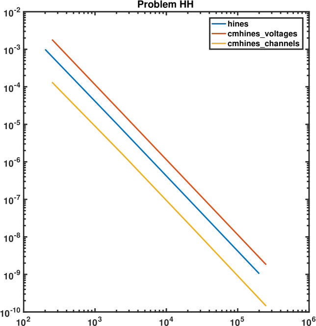
Figure 1: The Hodkin-Huxley system: Constant step size solvers

(a)	(b)

The Hodkin-Huxley system: Comparison of solvers. (a) behavior of the new solvers in comparison to matlab’s ode solvers, (b) behavior of the new solvers with different assignments to the $x$- and $y$-components. The tags “voltages” and “channels” indicate which set of variables has been considered as $x$-components

(a)	(b)

The Hodkin-Huxley system: Comparison of solvers. (a) The new solvers and the constant step size Hines’ method, (b) state-of-the-art methods and the most efficient new version

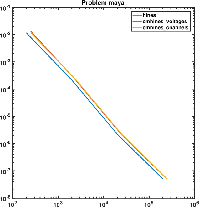
Figure 2: The soma-dendrite-spine system: Constant step size solvers

(a)	(b)

The soma-dendrite-spine system: Comparison of solvers. (a) behavior of the new solvers in comparison to matlab’s ode solvers, (b) behavior of the new solvers with different assignments to the $x$- and $y$-components. The tags “voltages” and “channels” indicate which set of variables has been considered as $x$-components

(a)	(b)

The soma-dendrite-spine system: Comparison of solvers. (a) The new solvers and the constant step size Hines’ method, (b) state-of-the-art methods and the most efficient new version

(a)	(b)

Tolerance-accuracy plots. (a) Hodgkin-Huxley model, (b) soma-dendrite-spine system

References

• [1] U.M. Ascher and L.R. Petzold. Coputer methods for Ordinary Differential Equations and Differential-Algebraic Equations. SIAM, Philadelphia, 1998.
• [2] J.M. Bower and D. Beeman. The Book of GENESIS: Exploring realistic neural models with the GEneral NEural SImulation System. Springer, 2nd edition, 1998.
• [3] M. Brandi. Simulating a Multi-Scale and Multi-Physics Model of a Dendritic Spine – Towards a communication framework for multi-scale modeling. Master thesis, KTH Royal Institute of Technology, 2011.
• [4] N.T. Carnevale and M.L. Hines. The NEURON Book. Cambridge University Press, 2005.
• [5] E. Hairer, S. Norsett, and G. Wanner. Solving ordinary differential equations I, volume 8 of Springer Series in Computational Mathematics. Springer, Berlin, 2. rev. edition, 1992.
• [6] E. Hairer and G. Wanner. Solving ordinary differential equations II, volume 14 of Springer Series in Computational Mathematics. Springer, Berlin, 2. rev. edition, 1996.
• [7] A.C. Hindmarsh, P.N. Brown, K.E. Grant, S.L. Lee, R. Serban, D.E. Shumaker, and C.S. Woodward. SUNDIALS, Suite of Nonlinear and Differential/Algebraic Equation Solvers. ACM Trans. Math. Software, 31:363–396, 2005.
• [8] M. Hines. Efficient computation of branched nerve equations. Int. J. Bio-Med. Comput., 15:69–76, 1984.
• [9] A.L. Hodgkin and A.F. Huxley. A quantitative description of membrane current and application to conduction and excitation in nerve. J. Physiol., 117:500–544, 1952.
• [10] W. Hundsdorfer and J. Verwer. Numerical solution of time-dependent advection-diffusion-reaction equations, volume 33 of Springer Series in Computational Mathematics. Springer, 2003.
• [11] W.H. Hundsdorfer and J.G. Verwer. Stability and convergence of the Peaceman- Rachford ADI method for initial-boundary value problems. Math. Comp., 53(187):81–101, 1989.
• [12] Ch. Ludwig. ODE MEXfiles for Radau5, version 16.07.2013. Technical report, TU München, http://www-m3.ma.tum.de/foswiki/pub/M3/Software/ODEFiles/radau5.zip, 2013. last accessed 10/01/2017.
• [13] D.W. Peaceman and Jr. Rachford, H.H. The numerical solution of parabolic and elliptic differential equations. J. Soc. Indust. Appl. Math., 3:28–41, 1955.
• [14] R. Serban. sundialsTB, a MATLAB Interface to SUNDIALS. Technical Report UCRL-SM-212121, LLNL, 2005.
• [15] G. Söderlind. Automatic control and adaptive time-stepping. Numer. Algorithms, 31:281–310, 2002.
• [16] G. Söderlind. Digital filters in adaptive time-stepping. ACM Trans. Math. Software, 29:1–26, 2003.
• [17] G. Strang. On the construction and comparison of difference schemes. SIAM J. Numer. Anal., 5:506–517, 1968.
• [18] K. Strehmel and R. Weiner. Partitioned Runge-Kutta adaptive methods and their stability. Numer. Math., 45:283–300, 1984.
{sidewaysfigure}