Why Do Cascade Sizes Follow a Power-Law?

Abstract

We introduce random directed acyclic graph and use it to model the information diffusion network. Subsequently, we analyze the cascade generation model (CGM) introduced by Leskovec et al. [19]. Until now only empirical studies of this model were done. In this paper, we present the first theoretical proof that the sizes of cascades generated by the CGM follow the power-law distribution, which is consistent with multiple empirical analysis of the large social networks. We compared the assumptions of our model with the Twitter social network and tested the goodness of approximation.

1 Introduction

Each day billions of instant messages, comments, articles, blog posts, emails, tweets and other various mediums of communication are exchanged in the reciprocal, social relations. The study of the information propagation through network is more and more demanded. Such models of propagation are used to minimize transmission costs, enhance the security and prevent information leaks or predict a propagation of malicious software among the users [13].

When considering state-of-the-art models of information diffusion, the underlying network structure of a transmission is constructed based on the known connections (e.g., the graph of followers in the Twitter network). Here, we have discovered that the graph of information dissemination has noteworthy features, unexploited in the previous works. It has been well known that more active individuals in the network have more acquaintances [27]. We have conducted experiments confirming those observations in the information diffusion network and showed its underlying structure.

Our model of the information diffusion network explains power-law (or Pareto) distribution of the number of informed nodes (cascade size). This is a major improvement over the state-of-the-art models, which give predictions inconsistent with the real data [8]. Random power-law graphs may sufficiently describe the follower-followee relation in the social network [5], but these graphs may not necessarily characterize the medium of an information propagation. The results of our study will allow researchers to enhance their models of the information transmission and will enable them to develop a framework to validate these models.

1.1 Related Work

Up to the best of our knowledge this work presents the first theoretical analysis of the cascade size distribution using cascade generation to model the spread of the information in the social networks. The first experimental analysis has been conducted by Leskovec et al. [19]. They proposed a cascade generation model and simulated it on the dataset of blog links. Since then, the research on the cascade sizes has become a fruitful field (for more references see [23]).

Through study on an epidemiology and a solid-state physics, different models such as SIR (susceptible-infectious-recovered) or SIS (susceptible-infectious-susceptible) has been employed to model the dynamics of spread of the information. However, all of these models assume that everyone in the population is in contact with everyone else [3], which is unrealistic in large social networks.

The classical example of the modified spreading process incorporates the effect of a stifler [2]. Stiflers never spread the information even if they were exposed to it multiple times. Nevertheless, stiflers can actively convert other spreaders or susceptible nodes into stiflers. That complicated logic may lead to the elimination of the epidemic threshold  and has been actively developed [6].

In 2002 Watts [26] proposed exact solution of the global cascade sizes on an arbitrary random graph. Notwithstanding, this process of the information propagation called the threshold model is utterly different from cascade generation by Leskovec et al. [19] and does not fully explain the dynamics of modern social networks like the Twitter.

Iribarren et al. [13] have developed the similar model, where an integro-differential equations have been introduced. That equations describe the cascade sizes when the number of messages send by a node is described by the Harris discrete distribution.However, the general solution to their equations is not known and merely solutions for nontrivial cases (e.g., superexponential processes [13]) has been considered. Our discoveries provide much simpler method and lucidly explain, that the underlying social graph is far more complex than just the graph of followers.

Results similar to ours were also obtained in the study on the bias of traceroute sampling. Achlioptas et al. [1] characterize the degree distribution of a BFS tree for a random graph with a given degree distribution. Their explanation why the degree distribution under traceroute sampling exhibits power-law motivated researchers to study bias in P2P systems [25] and network discovery [4]. Their research also resulted in the development of the new tools in the social networks sampling [16].

In the seminal paper of Leskovec et al. [18], the cascade size distribution in the network of recommendation has been analyzed. Leskovec et al. [18] showed that the product purchases follow a “long tail” distribution, where a significant fraction of sold items were rarely sold items. They fit the data to the power-law distribution and discovered, that the parameters may differ for distinct networks (remarkably, the power-law exponent was close to $-1$ for DVD recommendation cascades).

One of the greatest issue in analyzing the cascade size distribution is the lack of a good theoretical background for this process. Recently, researchers [20] has presented new models, designed to fit real distribution of cascade sizes. Moreover, goodness of fit test against CGM model has been conducted. It turns out, that CGM works well for small cascades, however it is unreliable for the large ones. The introduction of time dependent parameters significantly improves predictions for the large cascades [20].

In future, theoretical studies on cascades size distribution could explain phenomena in Gossip-based routing [10], rumor virality and influence maximization [14], recurrence of the cascades [7] or assist in forecasting rumors [15]. Currently the research in this area is purely empirical and we need more theoretical models to understand the process of information propagation [20].

2 Modeling Information Cascades

Intuitively, information cascades are generated by the following process: one individual passes the information to all its acquaintances. Then in each round newly informed nodes randomly decide to pass it to their acquaintances. This process continues until no new individuals are informed. The graph generated by the spread of the information is called the cascade.

The cascade generation model (CGM) established by [19] introduces a single parameter $\alpha$ that measures how infectious a passed information is. More precisely, $\alpha$ is the probability that the information will be passed to the acquaintance.

According to Leskovec et al. [19], the cascade is generated by the following:

1. Uniformly at random pick a starting point of the cascade and add it to the set of newly informed nodes.

2. Every newly informed node independently with the probability $\alpha$ informs their direct neighbors.

3. Let newly informed be the set of nodes that has been informed for the first time in step $2$ and add them to the generated cascade.

4. Repeat steps $2$ and $3$ until newly informed set is empty.

In this model we assume that all nodes have an identical impact ($\alpha=\mathrm{const}$) on their neighbors and all generated cascades are trees, since we pick a single, initial node. It is not a major problem, since the most of cascades are trees [19].

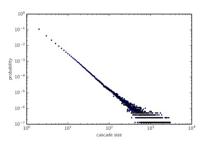
Figure 1: The log-log plot of the cascade size distribution on the Twitter dataset. It follows a power-law with an exponent $-2.3$.

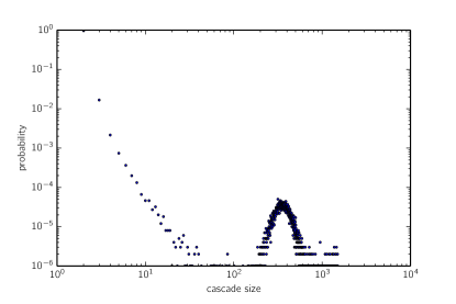
Figure 2: The log-log plot of the cascade size distribution predicted by the simulation of CGM using the Twitter followers graph. Note the phase transition, absent in real data.

Recently, information diffusion models have been evaluated on large social networks and it has been observed [24, 8] that the actual cascade size distribution is inconsistent with the distribution predicted by the model. First, the simulation registered an obvious phase transition (the cascades are either extremely large or are smaller than $100$) (see Figure 2). No such gap has been observed in the real data (see Figure 1). Second, the probability of the large cascade is intolerably high in simulations. 

There has been many attempts to readjust the cascade generation model [11, 8, 17], but as we have discussed above, those attempts oversimplify the process or incorrectly describe the distribution of cascades sizes. We introduce novel observations concerning the underlying social network and based on them we introduce a theoretical model of information propagation.

2.1 Information Transmission

The underlying network of rumor spreading is unknown. Even if we would have the network of all social contacts, the rumor could propagate through the mass media with a random interaction or even evolve in time. Because of that, when analyzing the social media we focus on the network of information propagation. The same technique has been used by Leskovec et al. [19], but their network was generated by links in blogs. To observe a non-trivial structure of the social network we considered actions generated by replying to messages. Such replies in the Twitter microblogging network are called retweets. We analyzed a set of over 500 millions tweets and the retweets from a $10\%$ sample of all tweets from May 19 to May 30 2013. Each retweet contains identifiers of the cited and replying users. Based on that, we generate a directed graph of the information transmission (same as [27, 8]). We use data published in [20, 22] and publish our code and experimental results on [21].

It is well known that the degree distribution of the generated graph follows a power-law [5]. However, this characterization does not necessarily describe the network of the information transmission. The intuition is that the nodes with greater degree are more active. Hence, when information spreads through the underlying network the distribution of spreading nodes should prefer nodes with higher degree, in consequence inflating the probability for these nodes.

Moreover, we have observed the hierarchical structure of the graph of retweets. The probability that a popular blogger replies to the message of an unpopular one is extremely small.

To confirm our intuition, we have determined the distribution of neighboring degrees for all nodes with a given degree. As shown on Figure 3 each degree has a distinct distribution of neighbors’ degrees (implementation is available on [21]). It means that it is more likely that a node is followed by some popular nodes when node itself is popular. Moreover, there is a pattern: the probability decreases with degree (for followers with degree greater than the followed node). Based on this observation we will model the aforementioned distribution as an approximated step function. This observation is consistent with the state-of-the-art analysis [19] and the most of cascades are “tree-like” or “stars”. According to our knowledge no further research has been conducted for examining distributions of neighbors degrees for node with a given degree (only cumulative degree for every cascade has been studied [19]).

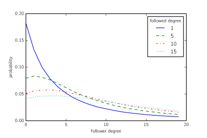
Figure 3: The degree distribution of the followers aggregated by the followed degree. Note the inflection point increases with a followed degree.

Undoubtedly, the process of information transmission in social networks is far more complex to be modeled by simulations just on the random power-law graphs. Because of the hierarchical structure and the relation of activity with node degree effects, we propose the model where the information is spread only to the nodes with lower degree with approximately uniform distribution.

2.2 Random DAG Generator

One of the basic methods for generating random graphs has been introduced in 1960 by Erdős and Rényi [9]. In a nutshell: for a given set of vertices, all edges have the same probability of being present or absent in a graph. This model of the graph is not suited for modeling the social networks because its degree distribution does not follow a power-law. The distribution of degrees for Erdős-Rényi model is binomial.

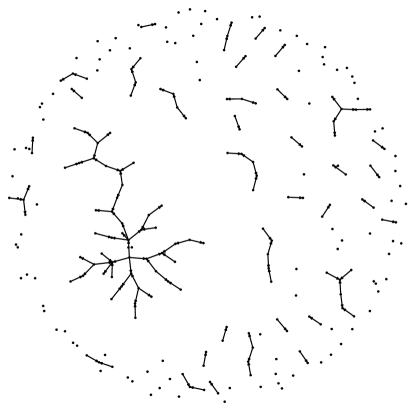
Figure 4: A diffusion network generated by the random DAG algorithm (see Algorithm 1).

This model is used in the theoretical research for modeling interactions between networks and propagation of catastrophes [12]. Even though Erdős-Rényi model does not characterize connections between nodes, we believe it can represent the process of information spreading. We will propose the intuitive variation of Erdős-Rényi model for directed graphs.

According to Leskovec et al. [19] the cascades very rarely express cycles and can be modeled as a tree-like structure. Even though this graphs do not model relationships in the social network, the directed acyclic graphs (DAG) are appropriate structure of the information propagation in the social network.

We introduce the procedure that generates the random directed acyclic graphs (DAG) and prove that propagating information in CGM regime results in cascade sizes obeying the power-law.

Let us denote by rdag$(n,p)$ a random graph generated by the RandomDAG($n,p$) (see Algorithm 1).

Algorithm 1 Generation of a random DAG

procedure RandomDAG($n,p$)

     $G\leftarrow\text{empty graph with vertices }1,2,\ldots,n$

     for $i\leftarrow 1\text{ to }n-1$ do

         for $j\leftarrow i+1\text{ to }n$ do

              with probability $p$ add directed edge $(j,i)$ to $G$

         end for

     end for

     return $G$

end procedure

The final $n$-vertices graph is acyclic since all edges $(j,i)$ obey $j>i$ (see Figure 5).

Any DAG can be generated by the RandomDAG($n,p$) when $p\in(0,1)$. If we label all vertices from $n$ to $1$ in the topological order, the graph $G$ will consist only of edges $(j,i)$ that $j>i$. Finally, all edges obeying $j>i$ can be present in the graph with independent probability $p$.

Figure 5: Sample DAG generated by procedure RandomDAG($5,p$). Dotted edges are unchosen.

Leskovec et al. [19] suggested that in the real information diffusion network, the small and simple graphs will occur more often than the complex, non trivial DAGs. This is exactly the case in RandomDAG($n,p$).

2.2.1 Degree Distribution of a Random DAG

The distribution of in-degrees in the rdag$(n,p)$ satisfies:

$$\mathbb{P}\left[\mathrm{indeg}(v)=k\right]=\frac{1}{n}\sum^{n-1}_{i=k}\binom{i}{k}p^{k}(1-p)^{i-k}.$$ (1)

Similarly to the Erdős-Rényi graph, the in-degree distribution of a given vertex $i$ is binomial but with different parameters for each node. As a consequence, it leads to a step-function like shape (see Figure 6).

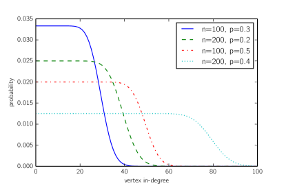
Figure 6: The in-degree distribution of the rdag$(n,p)$ graphs, according to Formula (1).

The in-degree distribution is almost uniform when the in-degree is lower than $np$. Naturally, this is merely a simple approximation of the true network of a probable information transmission. Still, based on observations in Section 2.1 rdag$(n,k)$ is the more accurate model than the follower-followee graph.

2.2.2 Comparison with Erdős-Rényi Model

The random DAG, in contrast to the standard Erdős and Rényi graph is a directed graph. It means that it can model one-way communication and the distribution of degrees. Next key difference is the hierarchical structure (i.e., the node $n$ will not follow the node with the lower label). These differences enable the random DAG model to produce cascades with the power-law distribution of sizes.

3 Analysis

In this section, we will formally analyze the introduced model. Subsequently, we will quantitatively describe a process of the information diffusion on a random DAG by determining the cascade size distribution.

Recall $p$ to be the probability of an edge in a rdag$(n,p)$ and $\alpha$ to be the average infectiousness of an information. Then set $\beta=1-p\alpha$ for simplicity. Hence, $\beta$ is the probability that the informed user will not spread the information through a given edge.

Now we will determine the probability $P_{n,k}$, that the cascade reaches $k$ distinct vertices in a graph with $n$ nodes, commencing from the vertex no. $1$. Clearly $P_{1,1}=1$ and $P_{n,k}=0$ when $k>n$ or $k\leq 0$. For a remaining case assume the cascade has size $k$ and consider two distinct states of the $n$-th node:

• $n$ was informed. Then, at least one of the other $k-1$ informed nodes had passed it to the $n$-th node, so the probability is $(1-\beta^{k-1})\cdot P_{n-1,k-1}$.

• $n$ was not informed. It can happen only when none of the other $k$ informed nodes passed the information to $n$-th node. The probability of such event equals $\beta^{k}\cdot P_{n-1,k}$.

Hence, we obtain a formula when $1\leq k\leq n$:

$$P_{n,k}=\beta^{k}\cdot P_{n-1,k}+(1-\beta^{k-1})\cdot P_{n-1,k-1},$$

To determine the distribution of the cascade size, we assume that an information shall commence in any node with an equal probability. Because the process of propagating the information in rdag$(n,p)$ starting from node $1$ is identical to propagating it from node $i$ in rdag$(n+i-1,p)$, the distribution is:

$$\mathbb{P}\left[|\emph{Informed}|=k\right]=S_{n,k}=\frac{1}{n}\sum_{i=1}^{n}P_{i,k}.$$

Now, we have the exact equation for the cascade size distribution. This equation does not have a simple form. However, we can ask what will happen when the number of nodes in graph is large. Let us recall that two series $x_{n},y_{n}$ are asymptotically equivalent when:

$$x_{n}\sim y_{n}\text{ iff }\lim_{n\to\infty}\frac{x_{n}}{y_{n}}=1.$$

The cascade size distribution satisfies Theorem 1.

Theorem 1

$$S_{n,k}\sim\frac{1}{n(1-\beta^{k})}$$

Proof 3.2.

Let us denote $\widetilde{S}_{n,k}=nS_{n,k}$. We need to prove that:

$$A_{k}:=\lim_{n\to\infty}\widetilde{S}_{n,k}=\frac{1}{1-\beta^{k}}.$$ (2)

We will prove it by induction. For $k=1$:

$$\widetilde{S}_{n,1} = \sum_{i=1}^{n}P_{i,1}=P_{1,1}+\sum^{n-1}_{i=1}P_{i+1,1}=1+\sum^{n-1}_{i=1}\beta P_{i,1}$$

$$= 1+\beta\widetilde{S}_{n-1,1}=1+\beta+\beta^{2}+\ldots+\beta^{n-1}.$$

Hence, $\widetilde{S}_{n,1}$ is the sum of the geometric series:

$$\widetilde{S}_{n,1}=\frac{1-\beta^{n}}{1-\beta}\to\frac{1}{1-\beta}.$$

For $k>1$:

$$\widetilde{S}_{n,k}=\sum_{i=1}^{n}P_{i,k}=\sum_{i=1}^{n}\beta^{k}P_{i-1,k}+\sum_{i=1}^{n}(1-\beta^{k-1})P_{i-1,k-1}.$$

So $\widetilde{S}_{n,k}$ obeys the recursive formula:

$$\widetilde{S}_{n,k}=\beta^{k}\widetilde{S}_{n-1,k}+(1-\beta^{k-1})\widetilde{S}_{n-1,k-1}.$$ (3)

Technical induction shows, that the $\widetilde{S}_{n,k}$ is bounded and increasing in respect to $n$, so $A_{k}=\lim_{n\to\infty}\widetilde{S}_{n,k}$ exists. Hence, we can take a limit on both sides of Equation 3 and obtain:

$$A_{k}=\beta^{k}A_{k}+(1-\beta^{k-1})A_{k-1},$$

$$A_{k}=\frac{1-\beta^{k-1}}{1-\beta^{k}}A_{k-1}.$$ (4)

Finally, by unwinding the recursive Formula (4), for each $k>0$ we obtain (recall that $A_{1}=\frac{1}{1-\beta}$):

$$A_{k}=\frac{1-\beta^{k-1}}{1-\beta^{k}}\frac{1-\beta^{k-2}}{1-\beta^{k-1}}\cdots\frac{1}{1-\beta}=\frac{1}{1-\beta^{k}}.$$

Hence, we have proved an asymptotic Formula (2) of the cascade size distribution.

3.1 Approximation for the Large Networks

Recall, that $\beta=1-p\alpha=1-\epsilon$. Because $p$ and $\alpha$ are extremely small, $\beta$ is close to 1. Taking the Laurent series of our function we get:

$$\frac{1}{1-(1-\epsilon)^{k}}=\frac{1}{k\epsilon}+\frac{k-1}{2k}+O(\epsilon).$$

The social networks have an extremely large number of nodes (e.g., the Twitter network has about $300$ millions distinct users [5]). On the other hand, new information reaches only few nodes (the cascade size distribution is believed to be a power-law for $k$ smaller than $10\,000$) [8, 19]. Then, because the element $\frac{k-1}{2kn}$ is insignificant when $n$ is that large, for $k\ll\frac{1}{p\alpha}\ll n$ we get:

$$S_{n,k}\sim\frac{1}{n(1-(1-p\alpha)^{k})}=\frac{1}{knp\alpha}+\frac{k-1}{2kn}+O(\frac{p\alpha}{n})$$

Hence, the distribution of cascade size:

(5)

in the first-order perturbation follows the power-law. Due to the low number of the large cascades, the distribution of sizes is unknown for $k$ close to $\frac{1}{p\alpha}$. In that case, one should use an exact formula.

3.2 Goodness of the Approximation

On the Figure 7 we have presented a comparison between approximation and exact formula for the distribution of cascade sizes. For a relatively small cascade size $k$ the slope of a distribution matches ideally.

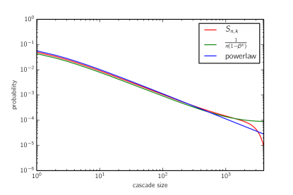
Figure 7: The log-log plot of an exact formula $S_{n,k}$, asymptotic bound $\frac{1}{n(1-\beta^{k})}$ and the power-law distribution with exponent $-1$.

How large cascades can we model using the aforementioned assumptions? The number of nodes $n$ in the Twitter network is approximately 300 millions. In [27] the average infectiousness $\alpha$ of the information on Twitter is said to be of order of $0.01$. According to Leskovec et al. [19], the number of edges in a cascade is proportional to $n^{1.03}$. So the parameter $p$ should be approximately $p\propto\frac{n^{1.03}}{n^{2}}$, since the number of possible edges is $n^{2}$. The largest rumor in our dataset has roughly $70\,000$ informed nodes, hence the lower bound for parameter $p$ is of order of $\frac{(7\cdot 10^{4})^{1.03}}{(7\cdot 10^{4})^{2}}\approx 2\cdot 10^{-5}$.

Still, $\frac{1}{\alpha p}\approx 5\cdot 10^{6}\ll 3\cdot 10^{8}\approx n$. So, for the Twitter network we can model the cascades with sizes $k\ll 5\cdot 10^{6}$. Remarkably, it is enough, since approximately $10^{-5}$ of Twitter rumors have the size greater than $10^{4}$.

3.2.1 Goodness of Fit

K-S test comparing the power-law distribution and the real cascade size distribution [22] is $0.0145$. At [20], the the K-S test comparing the cascade size distribution on the variant of CGM with real cascade distribution is $0.0447$. It means, that our model can potentially improve the test value by $3\%$ in comparison to the CGM on the graph of retweets.

3.3 Other Schemes of Information Diffusion

One would state that cascade generation model is counterintuitive for microblogging services such as the Twitter. In fact, it is more intuitive that every follower of the spreader eventually will be informed. So every follower, after being informed for the first time ought to make exactly one decision (with probability $\alpha$): whether to pass the information to all of its acquaintances simultaneously (previously the information was passed to each of its followers independently and each follower may had multiple opportunities to become a spreader). In such a case, the Formula (5) is exactly the same (for further proof see Appendix A).

4 Conclusion and Future Work

The graph of the information diffusion is utterly different from the global network of social connections. In contrast to multiple previous approaches, we model the cascade of information propagation as the random directed acyclic graph and we show that in the scheme of CGM the distribution of information popularity is asymptotically equivalent to:

where $n$ is the number of nodes and $\beta$ is a parameter dependent on both infectiousness of average information and density of the cascade. We show that for a sufficiently big number of nodes this distribution follows the power-law, what is consistent with real world observations. We hope that an introduction of this framework will inspire the theoretical affords to model and describe the information diffusion in the large social networks. The analysis of the rdag$(n,p)$ graph showed that the cascade size distribution follows the power-law for $\gamma=-1$. Leskovec et al. [18] presented the rich family of data with power-law exponent close to $-1$. Leskovec et al. [18] suggest that the information propagation in the network of recommendations may produce cascades with desired exponent. However, in the real data, the parameter $\gamma$ can be completely different (e.g., see Figure 1 of the Twitter cascade size distribution with power-law exponent $\gamma=-2.3$). To adopt our rdag$(n,p)$ model to those cases, one can customize a distribution of random cascades (we assumed a fairly simple method to generate them). We believe that adaptation of cascade shape distribution to the experimental data will readjust the $\gamma$ parameter (for a start one can use the shape distribution provided by Leskovec et al. [19]). Further enhancements might also be achieved by adapting the information diffusion scheme to a particular society (similarly to Appendix A). To encourage other researchers to apply our model in practice, we publish the code used to generate all figures and the results on [21].

Still, we need more experiments and research to answer what type of social networks the random directed acyclic graphs model and how richer set of features (e.g., spatio-temporal features) influences the cascade size distribution.

5 Acknowledgments

This work was partially supported by NCN grant UMO-2014/13/B/ST6/01811, ERC project PAAl-POC 680912, ERC project TOTAL 677651, FET IP project MULTIPLEX 317532 and polish funds for years 2013-2016 for co-financed international projects.

Appendix A Dependant Passing of the Information

In this model we count spreaders who pass the information to all of theirs followers with probability $\alpha$. These followers will receive the information and might become new spreaders.

For clarity, we will use the notation from Section 3 and the proof of Theorem 1.

Analogously to previous analysis, we obtain the recursive formula:

$$P_{1,1} = \alpha,$$

$$P_{n,k} = 0,\text{ when }k>n,$$

$$P_{n,k} = \big{(}1-(1-\beta^{k})\alpha\big{)}\cdot P_{n-1,k}+\alpha(1-\beta^{k-1})\cdot P_{n-1,k-1}.$$

Rest of the proof is almost identical to the proof of Theorem 1.

For $k=1$, we have:

$$\lim_{n\to\infty}\widetilde{S}_{n,1}=\lim_{n\to\infty}\frac{1-\big{(}1-(1-\beta^{k})\alpha\big{)}^{n}}{1-\beta}=\frac{1}{1-\beta}.$$

For $k>1$, when $n\to\infty$:

$$\lim_{n\to\infty}\widetilde{S}_{n,k}=A_{k} = \big{(}1-(1-\beta^{k})\alpha\big{)}A_{k}+$$

$$+\alpha(1-\beta^{k-1})A_{k-1}.$$

By subtracting the expression on both sides:

$$A_{k}-A_{k}(1-(1-\beta^{k})\alpha)=A_{k-1}\alpha(1-\beta^{k-1}).$$

And after simplification we get:

$$A_{k}(1-\beta^{k})\alpha=A_{k-1}(1-\beta^{k-1})\alpha$$

Hence, we have obtained the same formula as in Theorem 1:

$$A_{k}=A_{k-1}\frac{1-\beta^{k}}{1-\beta^{k-1}}$$

and finally obtain:

$$\lim_{n\to\infty}\widetilde{S}_{n,k}=\frac{1}{1-\beta^{k}}.$$

References

- [1] D. Achlioptas, A. Clauset, D. Kempe, and C. Moore. On the bias of traceroute sampling: Or, power-law degree distributions in regular graphs. J. ACM, 56(4):21:1–21:28, 2009.
- [2] M. Barthelemy, A. Barrat, and A. Vespignani. The role of geography and traffic in the structure of complex networks. Advances in Complex Systems, 10(1):5–28, 2007.
- [3] N. Bayley. The mathematical theory of epidemics. Griffin, London, 1975.
- [4] Z. Beerliova, F. Eberhard, T. Erlebach, A. Hall, M. Hoffmann, M. Mihal’ak, and L. S. Ram. Network discovery and verification. IEEE Journal on selected areas in communications, 24(12):2168–2181, 2006.
- [5] P. Brach, M. Cygan, J. Lacki, and P. Sankowski. Algorithmic complexity of power law networks. In R. Krauthgamer, editor, Proceedings of the Twenty-Seventh Annual ACM-SIAM Symposium on Discrete Algorithms, SODA 2016, Arlington, VA, USA, January 10-12, 2016, pages 1306–1325. SIAM, 2016.
- [6] P. Brach, A. Epasto, A. Panconesi, and P. Sankowski. Spreading rumours without the network. In A. Sala, A. Goel, and K. P. Gummadi, editors, Proceedings of the second ACM conference on Online social networks, COSN 2014, Dublin, Ireland, October 1-2, 2014, pages 107–118. ACM, 2014.
- [7] J. Cheng, L. A. Adamic, J. M. Kleinberg, and J. Leskovec. Do cascades recur? In J. Bourdeau, J. Hendler, R. Nkambou, I. Horrocks, and B. Y. Zhao, editors, Proceedings of the 25th International Conference on World Wide Web, WWW 2016, Montreal, Canada, April 11 - 15, 2016, pages 671–681. ACM, 2016.
- [8] B. Cui, S. J. Yang, and C. Homan. Non-independent cascade formation: Temporal and spatial effects. In J. Li, X. S. Wang, M. N. Garofalakis, I. Soboroff, T. Suel, and M. Wang, editors, Proceedings of the 23rd ACM International Conference on Conference on Information and Knowledge Management, CIKM 2014, Shanghai, China, November 3-7, 2014, pages 1923–1926. ACM, 2014.
- [9] P. Erdős and A. Rényi. On the evolution of random graphs. In PUBLICATION OF THE MATHEMATICAL INSTITUTE OF THE HUNGARIAN ACADEMY OF SCIENCES, pages 17–61, 1960.
- [10] A. Gaba, S. Voulgaris, K. Iwanicki, and M. van Steen. Revisiting gossip-based ad-hoc routing. In WiMAN 2012: Proceedings of the 6th International Workshop on Wireless Mesh and Ad Hoc Networks, Munich, Germany, July 2012. IEEE.
- [11] R. Ghosh and B. A. Huberman. Ultrametricity of information cascades. CoRR, abs/1310.2619, 2013.
- [12] S. Havlin, N. A. M. Araujo, S. V. Buldyrev, C. S. Dias, R. Parshani, G. Paul, and H. E. Stanley. Catastrophic cascade of failures in interdependent networks. CoRR, abs/1012.0206, 2010.
- [13] J. L. Iribarren and E. Moro. Branching dynamics of viral information spreading. CoRR, abs/1110.1884, 2011.
- [14] D. Kempe, J. M. Kleinberg, and É. Tardos. Maximizing the spread of influence through a social network. In L. Getoor, T. E. Senator, P. M. Domingos, and C. Faloutsos, editors, Proceedings of the Ninth ACM SIGKDD International Conference on Knowledge Discovery and Data Mining, Washington, DC, USA, August 24 - 27, 2003, pages 137–146. ACM, 2003.
- [15] S. Krishnan, P. Butler, R. Tandon, J. Leskovec, and N. Ramakrishnan. Seeing the forest for the trees: new approaches to forecasting cascades. In W. Nejdl, W. Hall, P. Parigi, and S. Staab, editors, Proceedings of the 8th ACM Conference on Web Science, WebSci 2016, Hannover, Germany, May 22-25, 2016, pages 249–258. ACM, 2016.
- [16] M. Kurant, A. Markopoulou, and P. Thiran. On the bias of bfs (breadth first search). In Teletraffic Congress (ITC), 2010 22nd International, pages 1–8. IEEE, 2010.
- [17] K. Lerman and R. Ghosh. Information contagion: An empirical study of the spread of news on digg and twitter social networks. In W. W. Cohen and S. Gosling, editors, Proceedings of the Fourth International Conference on Weblogs and Social Media, ICWSM 2010, Washington, DC, USA, May 23-26, 2010. The AAAI Press, 2010.
- [18] J. Leskovec, L. A. Adamic, and B. A. Huberman. The dynamics of viral marketing. TWEB, 1(1), 2007.
- [19] J. Leskovec, M. McGlohon, C. Faloutsos, N. S. Glance, and M. Hurst. Patterns of cascading behavior in large blog graphs. In Proceedings of the Seventh SIAM International Conference on Data Mining, April 26-28, 2007, Minneapolis, Minnesota, USA, pages 551–556. SIAM, 2007.
- [20] A. Pacuk, P. Sankowski, K. Wegrzycki, and P. Wygocki. There is something beyond the twitter network. In J. Blustein, E. Herder, J. Rubart, and H. Ashman, editors, Proceedings of the 27th ACM Conference on Hypertext and Social Media, HT 2016, Halifax, NS, Canada, July 10-13, 2016, pages 279–284. ACM, 2016.
- [21] A. Pacuk, P. Sankowski, K. Węgrzycki, and P. Wygocki. Python code of experiments and results. http://social-networks.mimuw.edu.pl/#rdag, 2017.
- [22] A. Pacuk, P. Sankowski, K. Węgrzycki, and P. Wygocki. Twitter anonymised graph. http://social-networks.mimuw.edu.pl/#beyond, 2017.
- [23] E. M. Rogers. Diffusion of innovations. Free Press, 2010.
- [24] G. V. Steeg, R. Ghosh, and K. Lerman. What stops social epidemics? In L. A. Adamic, R. A. Baeza-Yates, and S. Counts, editors, Proceedings of the Fifth International Conference on Weblogs and Social Media, Barcelona, Catalonia, Spain, July 17-21, 2011. The AAAI Press, 2011.
- [25] D. Stutzbach, R. Rejaie, N. Duffield, S. Sen, and W. Willinger. On unbiased sampling for unstructured peer-to-peer networks. IEEE/ACM Transactions on Networking (TON), 17(2):377–390, 2009.
- [26] D. J. Watts. A simple model of global cascades on random networks. In Proceedings of the National Academy of Sciences of the United States of America, volume 99, pages 5766–5771, April 30 2002. http://www.jstor.org/view/00278424/sp020038/02x3936j/0.
- [27] Q. Zhao, M. A. Erdogdu, H. Y. He, A. Rajaraman, and J. Leskovec. SEISMIC: A self-exciting point process model for predicting tweet popularity. In L. Cao, C. Zhang, T. Joachims, G. I. Webb, D. D. Margineantu, and G. Williams, editors, Proceedings of the 21th ACM SIGKDD International Conference on Knowledge Discovery and Data Mining, Sydney, NSW, Australia, August 10-13, 2015, pages 1513–1522. ACM, 2015.