Quantum criticality of spinons

Abstract

The free fermion nature of interacting spins in one dimensional (1D) spin chains still lacks a rigorous study. In this letter we show that the length-$1$ spin strings significantly dominate critical properties of spinons, magnons and free fermions in the 1D antiferromagnetic spin-1/2 chain. Using the Bethe ansatz solution we analytically calculate exact scaling functions of thermal and magnetic properties of the model, providing a rigorous understanding of the quantum criticality of spinons. It turns out that the double peaks in specific heat elegantly mark two crossover temperatures fanning out from the critical point, indicating three quantum phases: the Tomonaga-Luttinger liquid (TLL), quantum critical and fully polarized ferromagnetic phases. For the TLL phase, the Wilson ratio $R_{W}=4K_{s}$ remains almost temperature-independent, here $K_{s}$ is the Luttinger parameter. Furthermore, applying our results we precisely determine the quantum scalings and critical exponents of all magnetic properties in the ideal 1D spin-1/2 antiferromagnet Cu(C₄H₄N₂)(NO₃)₂ recently studied in Phys. Rev. Lett. 114, 037202 (2015)]. We further find that the magnetization peak used in experiments is not a good quantity to map out the finite temperature TLL phase boundary.

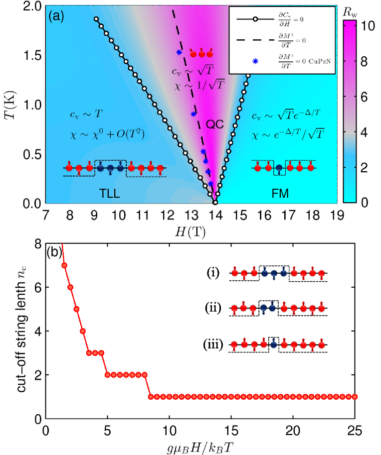
Figure 1: (a) Contour plot of the Wilson ration $R_{\mathrm{W}}$ in the $T-H$ plane. Without losing generality we used the realistic coupling constant $2J=10.81K$ and the Lande factor $g=2.3$ of the spin-1/2 compound CuPzN. It maps out quantum scalings of the TLL, the quantum critical (QC) region and the fully polarized ferromagnetic (FM) phase. The dotted solid lines fanning out from the saturation field $H_{s}=4J$ show the peak positions of the specific heat. The black dashed line shows the magnetization peaks determined from the TBA equations (S.4). The blue stars show the experimental magnetization peaks. (b) The cut-off string length $n_{c}$ versus the energy scale $g\mu_{B}H/(k_{B}T)$ at an accuracy of the order of $10^{-6}$. The cut-off $n_{c}$ shows stir-like features at low temperatures. The inset shows three schematic spin configurations: (i) $M^{z}=1$ and $2$ spinons; (ii) $M^{z}=0$, $\nu_{2}=1$ and $2$ spinons; (iii) $M^{z}=1$, $\nu_{2}=1$ and $4$ spinons, see Supp .

Of central importance to the study of the 1D spin-1/2 antiferromagnetic Heisenberg chain is the understanding of spin excitations Yang:1966a ; Faddeev:1981 ; Haldane:1981 ; Affleck:1986a ; Takahashi:1999 ; WangYP:2015 ; Johnston:2000 ; Tennant:1995 ; Lake:2005 ; Mourigal:435 ; Lake:2013 ; Zheludev:2008 ; Stone:2003 . Elementary spin excitations in this model may exhibit quasi-particle behaviour which is described by spinons carrying half a unit of spin. Such fractional quasiparticles are responsible for the TLL in the model Affleck:1986 ; Cardy:1986 ; Giamarchi:2004 .

Regarding to the Bethe ansatz solution of the 1D spin-1/2 chain, a significant development is Takahashi’s discovery of spin string patterns Takahashi:1971 , i.e., magnon bound states with different string lengths. Takahashi’s spin strings give one full access to the thermodynamics of the model through Yang and Yang’s grand canonical approach Yang:1969 , namely the so-called thermodynamic Bethe ansatz (TBA) equations Takahashi:1971 . However, the problems of how such spin strings determine the free fermion nature of spinons and how spin strings comprise universal scalings of thermal and magnetic properties still lack a rigorous understanding. In this paper we present a full answer to these questions.

Using spin string solutions to the TBA equations, we obtain the following results: I) we obtain exact scaling functions, critical exponents and a benchmark of quantum magnetism for the 1D spin-1/2 Heisenberg chain, revealing the microscopic origin of the quasiparticle spinons, free fermions and magnons that emerge in different physical regimes; II) We find that the Wilson ratio Som28 ; Wil75 , the ratio between the susceptibility $\chi$ and the specific heat $c_{v}$ divided by the temperature $T$, $R_{\mathrm{W}}=\frac{4}{3}\left(\frac{\pi k_{B}}{g\mu_{B}}\right)^{2}\chi/(c_{v}/T)$, significantly characterises the TLL of spinons and marks the crossover temperature between the quantum critical phase and the TLL Kono:2015 , see Fig. 1. When the magnetic field is larger than the saturation field, dilute magnon behaviour is evidenced by the exponential decay of the susceptibility; III) Using our analytical and numerical results we precisely determine the quantum scalings and magnetic properties of the ideal spin-1/2 antiferromagnet Cu(C₄H₄N₂)(NO₃)₂ (denoted by CuPzN for short) Kono:2015 . We also find that the magnetization peak used in experiment Kono:2015 ; Ruegg:2008 ; Shaginyan:2016 is not a good quantity to map out the finite temperature TLL phase boundary. Instead one should use the Wilson ratio or the specific heat peaks.

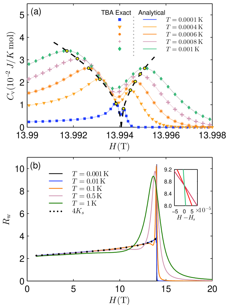
Figure 2: (a) Numerical (symbols from (S.4)) and analytical (solid lines from (5)) specific heat versus magnetic field in the same setting as that of Fig. 1. The double-peaks (circles) fanning out from the $Hs=13.9941$(T) mark the crossover temperatures separating the three regions: the TLL, the QC and the FM, see Fig 1. (b) A numerical plot of the Wilson ratio at different temperatures, which collapse to the Luttinger parameter curve of $4K_{s}$ calculated using (S.4), indicating the TLL nature. The inset shows the dimensionless scaling behaviour of the Wilson ratio at low temperatures.

Bethe ansatz equations. The Hamiltonian of the 1D Heisenberg spin 1/2 chain is given by Bethe:1931

$$\mathcal{H}=2J\sum_{j=1}^{N}\vec{S}_{j}\cdot\vec{S}_{j+1}-g\mu_{B}HM^{z},$$ (1)

where $J$ is the intrachain coupling constant, $N$ is the number of lattice sites and $M^{z}=\sum_{j=1}^{N}S_{j}^{z}=N/2-M$ is the magnetization. $M$ is the number of down spins. In this Hamiltonian, $g$ and $\mu_{B}$ are the Landé factor and the Bohr magneton, respectively. To simplify notation, we let $g\mu_{B}=1$. The spin-1/2 operator $\vec{S}_{j}$ associate to the site $j$ interacts with its nearest neighbours under a magnetic field $H$. The energy is given by $E=-\sum^{M}_{j=1}\frac{J}{\lambda_{j}^{2}+\frac{1}{4}}+HM+E_{0}$, where $E_{0}=\frac{1}{2}N\left(J-H\right)$, and the spin quasimomenta $\lambda_{j}$ with $j=1,\ldots,M$ are determined by the Bethe ansatz (BA) equations Bethe:1931 ; Takahashi:1999 , also see Supp . For the ground state, all the $\lambda_{j}$ take real values. However, at finite temperatures and in the thermodynamic limit, there are real and complex solutions describing different lengths of bound states

$$\lambda^{n}_{j,\ell}=\lambda^{n}_{j}+\frac{1}{2}\mathrm{i}(n+1-2\ell)$$ (2)

with $\ell=1,\ldots,n$, and $j=1,\ldots,\nu_{n}$. Here $\lambda^{n}_{j}$ and $\nu_{n}$ denote the real part and the number of length-$n$ strings, respectively Faddeev:1981 .

Building on such spin strings Takahashi:1971 , the thermodynamics of the system is determined by the TBA equations

$$\varepsilon_{n}^{+}=\varepsilon^{0}_{n}-\sum_{m}A_{m,n}\ast\varepsilon_{m}^{-}(\lambda),$$ (3)

where $\ast$ denotes convolution, $n$ takes positive integer values and $\varepsilon_{n}^{\pm}=\pm T\ln[1+{\rm e}^{\pm\varepsilon_{n}/T}]$ defines the dressed energy of the length-$n$ spin strings. The driving term is given by $\varepsilon_{n}^{0}=-2\pi Ja_{n}(\lambda)+nH$ with the kernel function $a_{n}(\lambda)=\frac{1}{2\pi}\frac{n}{\lambda^{2}+n^{2}/4}$. The function $A_{m,n}$ is given in Supp . The free energy per unit length is given by $f=\sum_{n}\int a_{n}\left(\lambda\right)\varepsilon_{n}^{-}\left(\lambda\right)d\lambda$. Hereafter, all magnetic properties will be in the per unit lengths.

Spin strings and spin liquid. For low-lying excitations, each magnon decomposes into two spinons, i.e. spin-1/2 quasiparticles Faddeev:1981 ; Hammar:1999 ; Karbach:2000 ; Karbach:2002 ; Caux:2005 ; Caux:2006 ; Klauser:2012 ; YangW:2017 . The spectral weight of two spinon excitations have been experimentally confirmed through observation of the spin dynamic structure factor Lake:2005 ; Mourigal:435 ; Lake:2013 ; Zheludev:2008 ; Stone:2003 . In order to calculate the spin string contributions to the thermodynamics at different temperature scales, we rewrite the free energy as $f=\sum_{n}g_{n}(\lambda)+\sum_{n}\varepsilon_{n}^{-}(\infty)$, where $g_{n}=\int{\rm d\lambda}\>a_{n}(\lambda)(\varepsilon_{n}^{-}(\lambda)-\varepsilon_{n}^{-}(\infty))$ counts the major contribution from the length-$n$ strings, besides their constant values $\varepsilon_{n}^{\pm}(\infty)$, to the free energy. Thus $g_{n}$ is very convenient for estimating the cut-off string length $n_{c}$, see Supp . It is important to observe that $g_{n}$ shows a power law decay as $n$ increases, see Fig. 1(b).

Here we observe that for a small value of $H/T$, a large cut-off string length $n_{c}$ is needed in the calculation of the thermodynamics. When $T\to\infty$, full string patterns are required, i.e. $n_{c}\to\infty$, so that the free energy reduces to that of free spins: $f=\sum_{n}\varepsilon_{n}^{-}(\infty)$. Moreover, for $H\sim 0^{+}$ and $T\ll 1$, logarithmic temperature corrections to the thermodynamical properties of the renormalization fixed point effective Hamiltonian have been seen Johnston:2000 ; Lukyanov:1998 ; Eggert:1994 . At $T=0$, all the $\lambda_{j}$ take real values. In this case, one easily gets the known magnetization critical exponent $\delta=2$ in the scaling form $1-M^{z}/M_{s}=D(1-H/H_{s})^{1/\delta}$ with $D=4/\pi$ Supp . This gives a divergent spin susceptibility at the saturation point $H_{s}=4J$ Bonner:1964 .

At low temperatures, i.e. $T\ll H$, the TLL feature is dominated by the excitations close to the Fermi points of the length-$1$ string $\varepsilon_{1}$ in the parameter $\lambda$ space. Such elementary excitations are described by particle hole excitations. From the TBA equations (S.4), the dressed energy $\varepsilon_{1}$ is given by $\varepsilon_{1}(\lambda)=\varepsilon_{1}^{(0)}(\lambda)+\eta(\lambda)+O(T^{3})$, where $\varepsilon_{1}^{(0)}(\lambda)$ is given by the dressed energy equation (S.4) in the limit $T=0$ and the leading order temperature correction is determined by $\eta(\lambda)=\frac{\pi^{2}T^{2}}{6t}[a_{2}(\lambda+Q)+a_{2}(\lambda-Q)]-\int_{-Q}^{Q}a_{2}\ast\eta(\mu){\rm d}\mu$. Here, $Q$ is fixed by the external field through $\varepsilon_{1}^{\left(0\right)}\left(\pm Q\right)=0$, see Supp . At low temperatures and in the limit of zero magnetic field, the free energy has been calculated by the Wiener-Hopf method Nepomechie:1993 . For arbitrary $H<H_{s}$, we thus obtain the field theory result for the free energy: $f=E_{0}-\pi T^{2}/(6v_{s})+O(T^{3})$, where $E_{0}$ is the ground state energy and the sound velocity is given by $v_{s}=\frac{1}{2\pi}\frac{d\varepsilon_{1}\left(\lambda\right)/d\lambda}{\rho_{0}\left(\lambda\right)}\mid_{\lambda=Q}$ Supp . This free energy gives the relativistic behavour of phonons Affleck:1986a , where the specific heat is $c_{v}/T=\pi/(3v_{s})$. This gives the dynamic critical exponent $z=1$.

Quantum criticality of spinons. In this spin-1/2 chain, the phase transition between the magnetized and ferromagnetic phases occurs at the saturation point Haldane:1981 ; Affleck:1986a ; Maeda:2007 . However, the determination of the phase boundary of the TLL at quantum criticality is still in question. In experiments Ruegg:2008 ; Kono:2015 , the magnetization peaks were regarded as the, as yet unjustified, TLL phase boundary. In Fig. 1 (a), we demonstrate that the peak positions of the specific heat( the dotted solid lines) fanning out from the saturation field $H_{s}$ coincide with the phase boundaries determined by the Wilson ratio $R_{\rm W}$. We observe that the phase boundary of the TLL determined by the magnetization peaks deviates significantly from the true TLL phase boundary as determined by the Wilson ratio and specific heat.

In Fig. 1 (a), we further demonstrate the existence of crossover temperatures from the double-peak structure of the specific heat. The existence of these crossover temperatures results in three different fluctuation regions: quantum and thermal fluctuations reach an equal footing (TLL); thermal fluctuations strongly coupled to quantum fluctuations (QC); dilute magnons dominate the fluctuations (FM). We show that there exists an intrinsic connection between the Wilson ratio and Luttinger parameter

$$R_{\mathrm{W}}=4K_{s}$$ (4)

for the Luttinger liquid, i.e. $H\leq H_{s}$, see Fig. 1(b). Here $K_{s}$ is the Luttinger parameter. A similar relation was recently found in spin ladder compounds and Fermi gases Nin12 ; GuaYFB13 ; Yu:2016 ; Saghafi:2016 . Thus the Wilson ratio elegantly quantifies the TLL regardless of the microscopic details of the underlying quantum system. This elegant relation (4) is confirmed by the numerical solutions of the TBA equations (S.4), see Fig. 1 (b). Moreover, the relation between the Luttinger parameter $K_{s}$ and the sound velocity $K_{s}=\pi v_{s}\chi/\left(g\mu_{B}\right)^{2}$ is also universal Giamarchi:2004 .

We further show that the length-$1$ spin strings dominate the quantum criticality of the antiferromagnetic spin-1/2 chain in the vicinity of the critical point Supp . We prove that the vanishing Fermi point gives rise to a universality class of free fermion criticality, i.e. the dilute spinons. By developing the generating function of free fermions in the TBA equations (S.4) Supp , we obtain the free energy

$$f \approx -\frac{2}{\pi}b_{1}+\frac{8}{\pi}b_{2}$$ (5)

near $H_{s}$, where $b_{1}=-\frac{\sqrt{\pi}T^{\frac{3}{2}}}{4\sqrt{J}}\operatorname{Li}_{\frac{3}{2}}\left(-e^{\frac{A}{T}}\right)$ and $b_{2}=-\frac{1}{2}\frac{\sqrt{\pi}T^{\frac{5}{2}}}{\left(16J\right)^{\frac{3}{2}}}\operatorname{Li}_{\frac{5}{2}}\left(-e^{\frac{A}{T}}\right)$ with $A=4J-H-\frac{b_{1}}{\pi}+\frac{b_{2}}{\pi}$. This simple result gives very accurate thermal and magnetic properties for the field near the saturation field, see 1(a). The polylog function $\operatorname{Li}_{3/2}(x)$ appearing in $b_{1}$ indicates that the spinons are similar in nature to free fermions. The magnon density $n_{\rm magnon}=M_{s}/N-M^{z}=\frac{\sqrt{2m^{*}T}}{\pi}\int^{\infty}_{0}\frac{dx}{e^{x^{2}-\frac{H_{s}-H}{T}}+1}$ can be obtained from (5) in the vicinity of the critical point. Here the effective mass of the magnon is given by $m^{*}\approx\frac{1}{2J}\left(1-\frac{T^{1/2}}{\sqrt{\pi J}}\int^{\infty}_{0}\frac{dx}{e^{x^{2}-\frac{H_{s}-H}{T}}+1}\right)$. We observe that the effective mass decreases as the magnetic field moves away from the critical point.

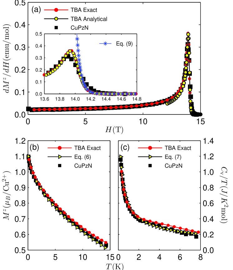
Figure 3: (a) Susceptibility versus magnetic field at $T=0.08$K. The numerical (red-dots (S.4)) and analytical (yellow-circles (5)) results agree well with the experimental measurement (black squares) for the 1D spin-$1/2$ antiferromagnet CuPzN Kono:2015 with the same setting used in Fig. 1. The inset shows the exponential decay of the susceptibility, as compared with Eq. (9), when the field slightly exceeds the saturation field $H_{s}$. (b) and (c) show the scaling laws of the magnetization and specific heat versus temperature. Excellent agreement is observed between our theoretical result and the experimental data (black-squares), where the red-dots and yellow-triangles denote the numerical TBA (S.4) result and the analytical scalings Eqs. (6) and (7), respectively.

Using the standard thermodynamic relations one can obtain entire scaling functions for the per unit length magnetization and the susceptibility for the region beyond the TLL, i.e. $T\gg H_{s}-H$:

$$M^{z} = \frac{1}{2}+\lambda_{0}T^{\frac{1}{2}}f^{s}_{\frac{1}{2}},\qquad\chi=-\lambda_{0}T^{-\frac{1}{2}}f^{s}_{-\frac{1}{2}},$$ (6)

where $\lambda_{0}=1/(2\sqrt{\pi J})$ and $f_{n}^{s}=\operatorname{Li}_{n}\left(-e^{\frac{\Delta}{T}}\right)$ with $\Delta=4J-H$. These analytical scaling functions signify the free fermion nature of the spinons and correspond to a dynamical critical exponent $z=2$ and a correlation length exponent $\nu=1/2$. In particular, the magnetization $(M_{s}/N-M^{z})/H\propto T^{\beta}$ determines the exponent $\beta=1/2$ in the critical region. The scaling function of the specific heat in the critical regime is given by

$$c_{v} = \sqrt{\frac{T}{\pi J}}\left[-\frac{3}{8}f^{s}_{\frac{3}{2}}+\frac{1}{2}\frac{\Delta}{T}f^{s}_{\frac{1}{2}}-\frac{1}{2}\left(\frac{\Delta}{T}\right)^{2}f^{s}_{-\frac{1}{2}}\right].$$ (7)

We see that $c_{v}/T\propto T^{-\alpha}$ with $\alpha=1/2$. By definition, the Wilson ratio in the critical region satisfies the scaling behaviour $R_{W}\approx\left(\frac{4\pi k_{B}}{3g\mu_{B}}\right)^{2}f_{-1/2}^{s}/f_{3/2}^{s}$ as $H\to H_{s}$. It follows that the Wilson ratio curves at low temperatures intersect, where the slopes are proportional to $1/T$, see the inset of Fig. 1 (b).

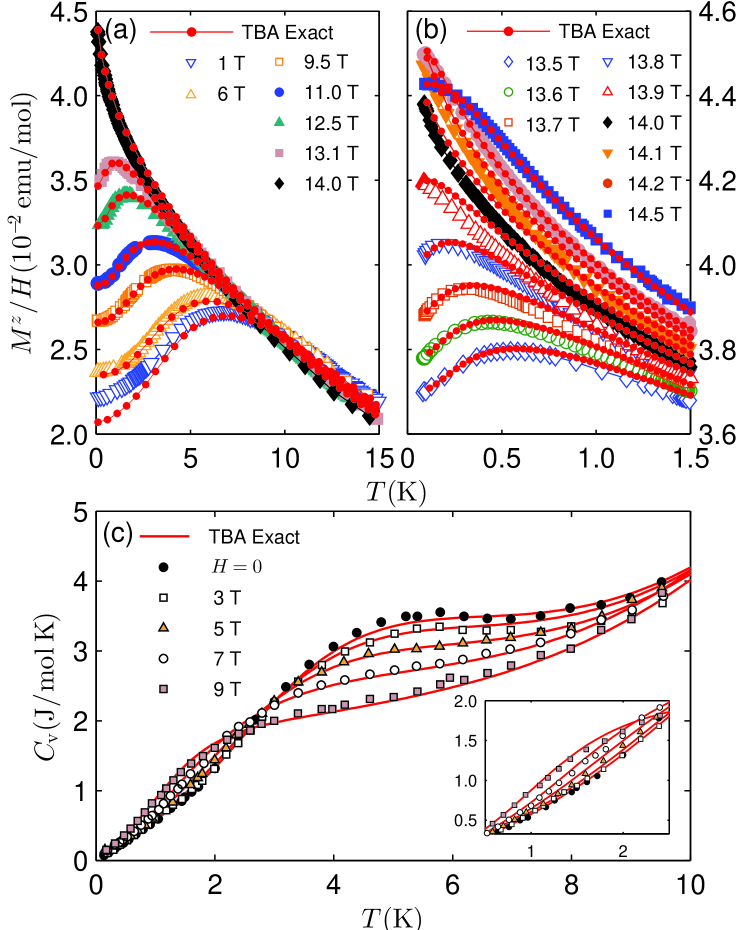
Figure 4: (a) Experimental magnetization $M^{z}/H$ versus temperature at various fields (see symbols) for the antiferromagnet CuPzN Kono:2015 . The red dots show the TBA numerical result with the same setting used in Fig. 1. For the case $H=1.0$T, we considered $n=120$ spin strings in order to reach a stable numerical accuracy. (b) shows the magnetization for low temperatures ($T\leqslant 1.5$K) and for magnetic fields near $H_{s}$, comparing the numerical result (red dots) with the experimental data (symbols). (c) Specific heat versus temperature for CuPzN Hammar:1999 with different magnetic fields. The symbols and solid red lines stand for the experimental and TBA numerical results from (S.4) with the cutoff string $n_{c}=30$. Here the phonon contribution is included. The inset shows the linear T-dependent signature within the curves as $T\to 0$.

So far, we have analytically obtained all critical exponents in the critical region:

$$\alpha=\beta=1/2,\,\,\delta=2,\,\,z=2,\,\,\nu=\frac{1}{2}.$$ (8)

They satisfy the relation $\alpha+\beta\left(1+\delta\right)=2$. In addition, when the magnetic field slightly exceeds the critical field $H_{s}$, the ferromagnetic ordering leads to a gapped phase where the susceptibility decays exponentially, illustrating the universal behaviour of the dilute magnons

$$\chi=\frac{1}{2\sqrt{\pi JT}}e^{-\Delta_{g}/T}$$ (9)

with $\Delta_{g}=4J-H$, see Fig. 3(a).

Application to the spin material. The analytical results obtained here for the quantum scaling functions (6)–(9) provide a precise understanding of the quantum criticality of the ideal spin-1/2 antiferromagnet CuPzN Kono:2015 , on which high precision measurements of the thermal magnetic properties have been made. Here the best fit of magnetic properties determines the coupling constant $2J=10.81$K, Lande factor $g=2.3$ and the saturation field $H_{s}=13.9941$(T) which only slightly differ from the experimental values $2J=10.8(1)$K, $g=2.3(1)$ and $H_{s}=13.97(6)$(T), respectively. Fig. 3(a) shows excellent agreement between our theoretical results for the susceptibility and the experimental data for the spin-1/2 antiferromagnet CuPzN in the measured region. In particular, one can identify dilute magnon behaviour for magnetic fields exceeding $H_{s}$, see the inset of Fig. 3(a). Indeed, the scaling forms of the susceptibility (6) and specific heat (7) fit quite well with the experimental data, see Fig. 3 (b) and (c). However, we mention a small discrepancy between the theoretical result and experimental data for the susceptibility in a narrow window around the critical point. This is due to a 3D coupling effect, which has also been noted in spin ladder compounds Klanjsek:2008 ; Thielemann:2009 ; Ruegg:2008 .

In Fig. 4 (a), (b), we have compared our theoretical calculations with experimental measurements for the magnetization of the antiferromagnet CuPzN subjected to both weak and strong magnetic fields. There was no theoretical examination on the magnetization data measured in this experiment Kono:2015 . Although there is overall agreement between our results and the data, an obvious discrepancy between theory and experiment was observed for $H\sim J^{{}^{\prime}}$ or $H_{s}-H\sim J^{{}^{\prime}}$ due to 3D interchain coupling. For this model $J^{{}^{\prime}}\approx 0.046$K, see the magnetization curves at $H=14.0$, $13.9$, $13.8$T in Fig. 4 (b). In addition, by properly choosing the cut-off string $n_{c}$, we can analyse the full thermodynamics of the model in the entire temperature regime by solving the TBA equation (S.4). In Fig. 4(c), for the specific heat, $n_{c}=30$ was used.

In summary, we have analytically obtained scaling functions and all the critical exponents of the thermal and magnetic properties of the spin-1/2 chain. This provides a rigorous theoretical understanding of the quantum criticality of spinons that has been observed in the antiferromagnet CuPzN Kono:2015 . We have found that the specific heat peaks elegantly mark the phase boundaries between the different phases at quantum criticality and that the Wilson ratio essentially quantifies the TLL and characterises phase transition regardless of the microscopic details of the systems. Our results also shed light on quantum liquids and the criticality of spinons in a variety of systems of interacting bosons and fermions with internal spin degrees of freedom.

Acknowledgments. The authors thank T. Giamarchi and H. Pu for helpful discussions. This work is supported by the NSFC under grant numbers 11374331 and the key NSFC grant No. 11534014. H.Q.L. acknowledges financial support from NSAF U1530401 and computational resources from the Beijing Computational Science Research Centre.

Supplementary materials: Quantum criticality of spinons
Feng He, Yu-Zhu Jiang, Yi-Cong Yu, H.-Q.Lin, and Xi-Wen Guan
 
 

I. Bethe ansatz and String hypothesis.

The Heisenberg spin-1/2 XXX chain is a prototypical integrable model, which is widely used to study quantum magnetism in one dimension (1D). In Hans Bethe’s seminal work Bethe , a particular type of wave function, which is called Bethe ansatz wave function, was proposed. Using this Bethe’s ansatz, the so-called Bethe ansatz (BA) equations and energy spectrum of the spin-1/2 XXX chain were given by

$$\left(\frac{\lambda_{j}-\frac{i}{2}}{\lambda_{j}+\frac{i}{2}}\right)^{2}=-\prod_{l=1}^{M}\frac{\lambda_{j}-\lambda_{l}-i}{\lambda_{j}-\lambda_{l}+i},$$ (S.1)

$$E(\lambda_{1},\cdots,\lambda_{M})=-\sum_{j=1}^{M}\left(\frac{J}{\lambda_{j}^{2}+\frac{1}{4}}\right)+HM+E_{0}.$$ (S.2)

Where $\lambda_{j}$ is spin quasimomentum with $j=1,\ldots,M$, and $M$ is the number of down spins.

The BA equations (S.1) determine the rapidities $\left\{\lambda_{j}\right\}$ which can be real and/or complex. The complex solutions of the Bethe roots are called spin strings by Takahashi Takahashi:1971

$$\lambda_{j,l}^{n}=\lambda_{j}^{n}+\frac{i}{2}(n+1-2l)$$ (S.3)

with $\ell=1,\ldots,n$, and $j=1,\ldots,\nu_{n}$, see the main text. In thermodynamic limit, i.e. $N,M\to\infty$, and $M/N$ is finite, and at finite temperatures, the grant canonical description gives rise to the so called thermodynamic Bethe ansatz (TBA) equations

$$\varepsilon_{n}^{+}=\varepsilon_{n}^{0}-\sum_{m}A_{m,n}\ast\varepsilon_{n}^{-}$$ (S.4)

with $n=1,2\ldots\infty$. The $\ast$ here denote convolution $(a\ast b)(\lambda)=\int_{-\infty}^{\infty}a(\lambda-\mu)b(\mu)d\mu$, and $\varepsilon^{\pm}=\pm T\ln(1+e^{\pm\varepsilon_{n}/T})$. The driving term is $\varepsilon_{n}^{0}=-2\pi Ja_{n}(\lambda)+nH=-\frac{nJ}{\lambda^{2}+n^{2}/4}+nH$ and the convolution kernel is

$$A_{m,n}\left(\lambda\right)=a_{m+n}\left(\lambda\right)+2a_{m+n-2}\left(\lambda\right)+\cdots+2a_{\left|m-n\right|+2}\left(\lambda\right)+a_{\left|m-n\right|}.$$ (S.5)

The full finite temperature thermodynamics can be determined from the per length free energy

$$f=\sum_{n}\int_{-\infty}^{\infty}a_{n}\left(\lambda\right)\varepsilon_{n}^{-}\left(\lambda\right)d\lambda.$$ (S.6)

II. Magnetism at zero Temparature.

From the form of TBA equations (S.4), we observe that $\varepsilon_{n}\geq 0$ for $n\geq 1$. Therefore, for $T=0$, the TBA equations and free energy per site reduce to

$$\varepsilon_{1}^{\left(0\right)}\left(\lambda\right) = -2\pi Ja_{1}\left(\lambda\right)+H-\int^{Q}_{-Q}a_{2}\left(\lambda-\mu\right)\varepsilon_{1}^{\left(0\right)}\left(\mu\right)d\mu,$$ (S.7)

$$f_{0} = \int^{+Q}_{-Q}a_{1}\left(\mu\right)\varepsilon_{1}^{(0)}\left(\mu\right)d\mu,$$ (S.8)

where the $Q$ is the cut-off spin quasimomentum determined by the zero point of dressed energy, i.e. $\varepsilon_{1}^{(0)}\left(\pm Q\right)=0$. The saturation magnetic field can be easily obtained from the condition $\varepsilon_{1}(0)=0$. This gives $H_{s}=4J$ and $M^{z}=1/2$. The zero temperature critical properties thus can be analytically obtained for a small $Q$ near the critical field $H_{s}$. We can expand the zero temperature TBA equation (S.7) in terms of $\lambda$, namely

$$\varepsilon_{1}^{(0)}(\lambda)\approx-2\pi Ja_{1}(\lambda)+H-\frac{1}{\pi}\int_{-Q}^{Q}\varepsilon_{1}^{(0)}(\lambda){\rm d}\lambda\approx-2\pi Ja_{1}(\lambda)+H-\frac{2Q(H-H_{s})}{\pi}.$$ (S.9)

Thus we get $Q=\sqrt{\frac{H_{s}-H}{16J}}$. The free energy, magnetization and susceptibility can directly evaluate with the zero temperature dressed energy

$$f_{0} \approx \int^{+Q}_{-Q}a_{1}\left(\mu\right)\varepsilon_{1}^{(0)}\left(\mu\right)d\mu\approx\frac{4J}{\pi}\frac{(1-4Q^{2})\arctan(2Q)-2Q}{1+4Q^{2}}+O(Q^{4}).$$ (S.10)

It follows that the normalized magnetization and magnetic susceptibility (in per length unit)

$$M^{z} = M_{s}-\frac{\partial f_{0}}{\partial H}=\frac{1}{2}-\frac{2}{\pi}\left(1-\frac{H}{H_{s}}\right)^{1/2},$$ (S.11)

$$\chi = \frac{\partial M^{z}}{\partial H}=\frac{1}{2\pi}\left(\frac{1}{J\left(H_{s}-H\right)}\right)^{1/2}.$$ (S.12)

Using this result, we give the scaling form

$$1-\frac{M^{z}}{M_{s}}=D\left(1-\frac{H}{H_{s}}\right)^{1/\delta}=\frac{4}{\pi}\left(1-\frac{H}{H_{s}}\right)^{1/2}$$ (S.13)

that reads off the critical exponent $\delta=2$ with the factor $D=4/\pi$ at zero temperature. This square-root behaviour of magnetization is showed in Fig. s1.

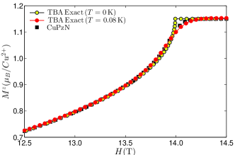
Figure s1: (color online). Per length magnetization $M^{z}$ vs external magnetic field $H$. The yellow-circles shows magnetization at zero temperature, which exhibits a square-root singularity at the saturation field $H_{s}=13.9941(T)$.

III. Spin strings.

The low-lying excitations of the spin-1/2 system are described by spin strings (S.3). These spin string patterns are very complicated under magnetic field and temperature. At zero magnetic field and zero temperature, real roots form the ground state of the spin-1/2 system. For the ground state Faddeev:1981 ; Caux:2005 ; Caux:2006 ; Klauser:2012 we regard the BA roots as $M=N/2$ magnons, i.e. $N/2$ length-1 spin strings to the BA (S.1) equations. Spin excitations are created by flipping the dow-spins so that a magnon decomposes into two spinons carried spin-1/2. Mathematically speaking, this spin flipping leads to two $\varepsilon_{1}(\lambda)$ holes in the sea of $\lambda$ roots of BA (S.1) equations. Such a two-spinon spectrum has been experimentally observed in many spin-1/2 systems. However, the spin excitations may lead to quite different spin string patterns, also see recent paper YangW:2017 . Here we demonstrate three simple low-lying excitations, see Fig. s2.

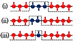
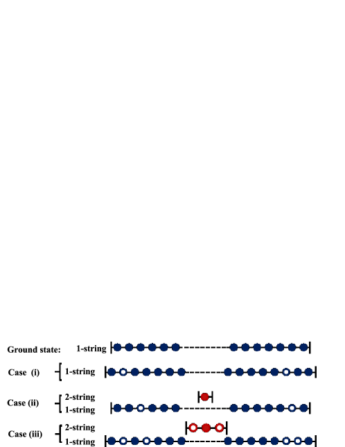
Figure s2: (color online). Schematic spin string configurations for (i) $M^{z}=1$ and $2$ spinons; (ii) $M^{z}=0,\nu_{2}=1$ and $2$ spinons; (iii) $M^{z}=1,\nu_{2}=1$ and $4$ spinons.

As being shown in Fig. s2, in order to give a clear picture on the elementary excitations, we prefer to use the Néel state to demonstrate spin excitations over the ground state at zero magnetic field .

Case (i): the two-spinon excitation with $M=N/2-1$ and the total spin $M^{z}=1$. In contrast to the ground state with $N/2$ magnons, this type of excitation has $N/2-1$ length-1 magnons and two holes, i.e. one magnon decomposes into two magnons. Such a spin flipping gives rise to two kinks ($\uparrow$-$\uparrow$), which are regarded as quasi-particles, i.e., two spinons. The two spinons move with two independent rapidities. In view of the BA equations, all vacancies are occupied for the ground state at zero magnetic filed. One less real string makes the number of total vacancies increased by one. Therefore, in this case, the excited states has two holes of length-$1$ string which form a scattering state of two spinons.

Case (ii): two-spinon excitation with $M=N/2$ and total spin $M^{z}=0$. In this spin singlet configuration, there is a length-$2$ string. Such a singlet excitation state is created by taking two length-$1$ strings out from the ground state pattern and add one length-2 string, see case (ii) in Fig. s2, where the two kinks ($\uparrow$-$\uparrow$ and $\downarrow$-$\downarrow$) are bounded together moving with one velocity. The length-2 string has only one vacancy. In terms of Bethe ansatz roots, we observe that there are two spinons in the length-1 string sector, which define the excitation energy. This indicates that the singlet excitation also splits into two spinons.

Case (iii): The spin triplet excitation with $M=N/2-1$ and total spin $M^{z}=1$. This spin triplet excitaion is constructed by taking three length-1 strings out form the ground state pattern and add one length-$2$ string with two holes (total three vacancies) in the length-$2$ sector, see case (iii) in Fig. s2, where the two $\uparrow$-$\uparrow$ kinks are bounded together. The only length-2 string occupies one of these three vacancies. These length-$2$ vacancies provide an order $\sim 1/N$ corrections to the momentum distributions and they are negligible in thermodynamic limit. Based on the root patterns of the BA equations, we observe that there are four spinons in the length-$1$ spin string sector. The excitation energy and momentum are determined by these four spinons in the thermodynamic limit.

The above configurations can be obtained from the TBA equations too. We assume that there are $v_{\nu}$ length-$\nu$ strings in the excited state. This configuration is created by taking $\gamma$ length-$1$ strings out of the ground state pattern. There is no other length spin strings, i.e. $v_{n}=0$ for $n\neq 1,\nu$. We assume that there are $\vartheta$ holes in length-$1$ string, located at $\lambda_{j}^{\rm h}$ with $j=1,2,\ldots,\vartheta$ and the density of holes in length-$1$ spin strings is $\rho_{1}^{\rm h}=\frac{1}{N}\sum_{j=1}^{\vartheta}\delta(\lambda-\lambda_{j}^{h})$. The $v_{\nu}$ length-$\nu$ strings locate at $\lambda^{\nu}_{i}$ with $i=1,2,\ldots,v_{\nu}$ and the corresponding density $\rho_{\nu}=\frac{1}{N}\sum_{i=1}^{v_{\nu}}\delta(\lambda-\lambda^{\nu}_{i})$. The density of particles and holes satisfy

$$\rho_{1}(\lambda)+\rho_{1}^{\rm h}(\lambda)=a_{1}(\lambda)-(a_{2}\ast\rho_{1})(\lambda)-\left((a_{\nu-1}+a_{\nu+1})\ast\rho_{\nu}\right)(\lambda).$$ (S.14)

Taking integration with respect to $\lambda$ on both sides of this equation, we get the number of spinons in the length-$1$ spin string sector

$$\vartheta=2(\gamma-v_{\ell}).$$ (S.15)

With the help of this equation, we can find the number of holes for different kinds of spin excitations as being discussed above. We can also calculate the excitation energies and momenta by using the TBA equations.

The spin strings configurations play important roles in quantum dynamic process at low temperatures. However, once we consider thermodynamics of the system at finite temperatures and finite magnetic field, contributions from different lengths of spin strings rather depend on numerical accuracy of the energy scales which we required. For example, in the vicinity of the saturation point, the length-$1$ strings of magnons dominate the critical behaviour. Different lengths of spin strings are requested to reach a certain accuracy of energy when the magnetic field and temperature are changed. We will further discuss the energy contributions from different spin strings later.

IV. Luttinger Liquid.

At low temperatures, the particle-hole excitations near two Fermi points form a collective motion which is called the Luttinger liquid. Such elementary excitations only involve the roots of length-$1$ strings. Despite of differences in microscopic details between the Luttinger liquids in 1D and Fermi liquid in higher dimensions, the particle-hole excitations in 1D lead to similar macroscopic behaviours of higher dimensional systems at low energy. The Luttinger liquid behaviour can be observed in the antiferromagnetic region with the condition $\left|H-H_{s}\right|/T\gg 1$. Without losing generality, we can rewrite the low temperature TBA equation (S.42) as $\varepsilon_{1}=\varepsilon_{1}^{\left(0\right)}+\eta$, where the $\varepsilon_{1}^{\left(0\right)}$ is zero temperature dressed energy (S.7) and $\eta$ can be regard as a leading order correction to the temperature, namely

$$\varepsilon_{1}\left(\lambda\right) = -2\pi Ja_{1}\left(\lambda\right)+H+T\int_{-\infty}^{\infty}a_{2}\left(\lambda-\mu\right)\ln\left(1+e^{\frac{-\varepsilon_{{}_{1}}\left(\mu\right)}{T}}\right)d\mu$$

$$= -2\pi Ja_{1}\left(\lambda\right)+H+T\left(\int^{-Q}_{-\infty}+\int^{\infty}_{Q}\right)a_{2}\left(\lambda-\mu\right)\ln\left(1+e^{\frac{-\varepsilon_{{}_{1}}\left(\mu\right)}{T}}\right)d\mu$$

$$+T\int^{Q}_{-Q}a_{2}\left(\lambda-\mu\right)\ln\left(1+e^{\frac{\varepsilon_{{}_{1}}\left(\mu\right)}{T}}\right)d\mu-\int^{Q}_{-Q}a_{2}\left(\lambda-\mu\right)\varepsilon_{1}\left(\mu\right)d\mu$$

$$= -2\pi Ja_{1}\left(\lambda\right)+H+T\int^{\infty}_{-\infty}a_{2}\left(\lambda-\mu\right)\ln\left(1+e^{\frac{-\left|\varepsilon_{{}_{1}}\left(\mu\right)\right|}{T}}\right)d\mu-\int^{Q}_{-Q}a_{2}\left(\lambda-\mu\right)\varepsilon_{1}\left(\mu\right)d\mu.$$

We then rewrite

$$\varepsilon_{1}\left(\lambda\right) = \varepsilon_{1}^{\left(0\right)}\left(\lambda\right)+\eta\left(\lambda\right)$$ (S.17)

$$= -2\pi Ja_{1}\left(\lambda\right)+H-\int^{Q}_{-Q}a_{2}\left(\lambda-\mu\right)\varepsilon_{1}^{\left(0\right)}\left(\mu\right)d\mu+\eta\left(\lambda\right)$$

$$= -2\pi Ja_{1}\left(\lambda\right)+H-\int^{Q}_{-Q}a_{2}\left(\lambda-\mu\right)\left(\varepsilon_{1}\left(\mu\right)-\eta\left(\mu\right)\right)d\mu+\eta\left(\lambda\right).$$

It follows that

$$\eta\left(\lambda\right) = T\int^{\infty}_{-\infty}a_{2}\left(\lambda-\mu\right)\ln\left(1+e^{\frac{-\left|\varepsilon_{{}_{1}}\left(\mu\right)\right|}{T}}\right)d\mu-\int^{Q}_{-Q}a_{2}\left(\lambda-\mu\right)\eta\left(\mu\right)d\mu$$ (S.18)

$$= I-\int^{Q}_{-Q}a_{2}\left(\lambda-\mu\right)\eta\left(\mu\right)d\mu$$

When $T\rightarrow 0,$ the dominant contribution to this integration comes from the regions near the Fermi points, i.e., the zeros of $\varepsilon_{1}$. By expanding $\varepsilon_{1}$ at $\lambda=Q$, we have

$$\varepsilon_{1}\left(\lambda\right)=t\left(\lambda-Q\right)+O\left(\left(\lambda-Q\right)^{2}\right)$$ (S.19)

with $t=\frac{d\varepsilon(\lambda)}{d\lambda}\Big{|}_{\lambda=Q}$. Then the first term of $\eta$ becomes

$$I = \frac{\pi^{2}T^{2}}{6t}\left[a_{2}\left(\lambda+Q\right)+a_{2}\left(\lambda-Q\right)\right].$$ (S.20)

Following a straightforward calculation, we have

$$\eta\left(\lambda\right)=\frac{\pi^{2}T^{2}}{6t}\left[a_{2}\left(\lambda+Q\right)+a_{2}\left(\lambda-Q\right)\right]-\int^{Q}_{-Q}a_{2}\left(\lambda-\mu\right)\eta\left(\mu\right)d\mu.$$ (S.21)

At zero temperature, the free energy per site $f\left(T,H\right)$ is given by

$$f_{0}\left(0,H\right)=\int^{Q}_{-Q}a_{1}\left(\lambda\right)\varepsilon_{1}^{\left(0\right)}\left(\lambda\right)d\lambda.$$ (S.22)

At low temperatures and zero magnetic field limit, the free energy was calculated by Wiener-Hopf method Nepomechie:1993 . Here we consider low temperatures and finite magnetic field. Under such conditions, the free energy is given by

$$f\left(T,H\right)=-T\int^{\infty}_{-\infty}a_{1}\left(\lambda\right)\ln\left(1+e^{\frac{-\varepsilon_{{}_{1}}\left(\lambda\right)}{T}}.\right)d\lambda.$$ (S.23)

It follows that

$$f-f_{0} = -T\int^{\infty}_{-\infty}a_{1}\left(\lambda\right)\ln\left(1+e^{\frac{-\varepsilon_{{}_{1}}\left(\lambda\right)}{T}}\right)d\lambda-\int^{Q}_{-Q}a_{1}\left(\lambda\right)\varepsilon_{1}^{\left(0\right)}\left(\lambda\right)d\lambda$$ (S.24)

$$= -T\left(\int^{-Q}_{-\infty}+\int^{\infty}_{Q}\right)a_{1}\left(\lambda\right)\ln\left(1+e^{\frac{-\varepsilon_{{}_{1}}\left(\lambda\right)}{T}}\right)d\lambda-T\int^{Q}_{-Q}a_{1}\left(\lambda\right)\ln\left(1+e^{\frac{\varepsilon_{{}_{1}}\left(\lambda\right)}{T}}\right)d\lambda$$

$$+\int^{Q}_{-Q}a_{1}\left(\lambda\right)\varepsilon_{{}_{1}}\left(\lambda\right)d\lambda-\int^{Q}_{-Q}a_{1}\left(\lambda\right)\varepsilon_{1}^{\left(0\right)}\left(\lambda\right)d\lambda$$

$$= -T\int^{\infty}_{-\infty}a_{1}\left(\lambda\right)\ln\left(1+e^{\frac{-\left|\varepsilon_{{}_{1}}\left(\lambda\right)\right|}{T}}\right)d\lambda+\int^{Q}_{-Q}a_{1}\left(\lambda\right)\eta\left(\lambda\right)d\lambda$$

$$= -\frac{\pi^{2}T^{2}}{3t}a_{1}\left(Q\right)+\int^{Q}_{-Q}a_{1}\left(\lambda\right)\eta\left(\lambda\right)d\lambda$$

Then we can express the free energy in terms of leading order contributions to the temperature

$$f=f_{0}-\frac{\pi^{2}T^{2}}{3t}a_{1}\left(Q\right)+\int^{Q}_{-Q}a_{1}\left(\lambda\right)\eta\left(\lambda\right)d\lambda$$ (S.25)

In order to get an close form of free energy, the key calculation is the last term in the Eq. (S.25). We use the spin-down density BA equation

$$\rho_{0}\left(\lambda\right)=a_{1}\left(\lambda\right)-\int_{-Q}^{Q}a_{2}\left(\lambda-\mu\right)\rho_{0}\left(\mu\right)d\mu$$ (S.26)

and the Eq. (S.21), we can obtain

$$\int^{Q}_{-Q}\frac{\pi^{2}T^{2}}{6t}\left[\left(a_{2}\left(\lambda+Q\right)+a_{2}\left(\lambda-Q\right)\right)\right]\rho_{0}\left(\lambda\right)d\lambda=\int^{Q}_{-Q}a_{1}\left(\lambda\right)\eta\left(\lambda\right)d\lambda.$$ (S.27)

Using the relation

$$\rho_{0}\left(Q\right) = a_{1}\left(Q\right)-\int^{Q}_{-Q}a_{2}\left(Q-\mu\right)\rho_{0}\left(\mu\right)d\mu,$$

$$\rho_{0}\left(-Q\right) = a_{1}\left(-Q\right)-\int^{Q}_{-Q}a_{2}\left(-Q-\mu\right)\rho_{0}\left(\mu\right)d\mu,$$ (S.28)

and summing up the two equations, we thus obtain

$$\int^{Q}_{-Q}\left[\left(a_{2}\left(\lambda+Q\right)+a_{2}\left(\lambda-Q\right)\right)\right]\rho_{0}\left(\lambda\right)d\lambda=2a_{1}\left(Q\right)-2\rho_{0}\left(Q\right).$$ (S.29)

Then we obtain the following result

$$\int^{Q}_{-Q}a_{1}\left(\lambda\right)\eta\left(\lambda\right)d\lambda=\frac{\pi^{2}T^{2}}{6t}\left[2a_{1}\left(Q\right)-2\rho_{0}\left(Q\right)\right].$$ (S.30)

Finally, together with the formula of the free energy per site (S.25), we give

$$f = f_{0}-\frac{\pi^{2}T^{2}}{3t}a_{1}\left(Q\right)+\int^{Q}_{-Q}a_{1}\left(\lambda\right)\eta\left(\lambda\right)d\lambda$$ (S.31)

$$= f_{0}-\frac{\pi^{2}T^{2}}{3t}a_{1}\left(Q\right)+\frac{\pi^{2}T^{2}}{6t}\left[2a_{1}\left(Q\right)-2\rho_{0}\left(Q\right)\right]$$

$$= f_{0}-\frac{\pi^{2}T^{2}}{3t}\rho_{0}\left(Q\right)\text{}.$$

We further define sound velocity

$$v_{s}=\frac{1}{2\pi}\frac{d\varepsilon_{1}\left(\lambda\right)/d\lambda}{\rho_{0}\left(\lambda\right)}\Big{|}_{\lambda=Q}=\frac{1}{2\pi}\frac{t}{\rho_{0}\left(Q\right)}.$$ (S.32)

We obtain the free energy per site with the leading order temperature correction

$$f=f_{0}-\frac{\pi T^{2}}{6v_{s}}$$ (S.33)

Since $f_{0}$ is the free energy per site at zero temperature, it is independent of $T$. It follows that the specific heat at TLL region is given by

$$c_{v}=-T\frac{\partial^{2}f}{\partial^{2}T}=\frac{\pi T}{3v_{s}}\propto T^{\alpha}.$$ (S.34)

This gives the exponent $\alpha=0$. In one dimension $\alpha=2-\left(d+z\right)/z$,$d=1$, so that the dynamic factor $z=1$.

Phenomenologically, the field theory Hamiltonian can be rewritten as an effective Hamiltonian in long wave length limit, which essentially describes the low energy physics of the spin chain Giamarchi:2004 , namely

$$H=\frac{\hbar}{2\pi}\int dx\left[\frac{v_{s}K_{s}}{\hbar^{2}}\left(\pi\Pi\left(x\right)\right)^{2}+\frac{v_{s}}{K_{s}}\left(\nabla\phi\left(x\right)\right)^{2}\right],$$ (S.35)

where the the canonical momenta $\Pi$ conjugate to the phase $\phi$ obeying the standard Bose commutation relations $\left[\phi(x),\Pi(y)\right]=\mathrm{i}\delta(x-y)$. In this approach, the density variation in space is viewed as a superposition of harmonic waves. The quantized harmonic waves are bosons (called bosonization) and form the new eigenstate of the 1D metallic state. In low energy excitations, the interaction between these quantized waves are marginal. The Luttinger parameter $K_{s}$ and the sound velocity $v_{s}$ characterize the low energy physics and determine long distance asymptotic of correlation functions. Therefore the effective Hamiltonian (S.35) captures the TLL physics of such kind.

For the spin-1/2 Heisenberg chain, in the bosonization language, the magnetization term $H_{m}=-g\mu_{B}HM^{z}$ in Hamiltonian can be written in term of the field $\partial_{x}\phi$

$$H_{m}=\frac{g\mu_{B}}{\pi}\int dxH\partial_{x}\phi$$ (S.36)

which is exactly the chemical potential term in the free spinless fermions. Using the TLL form of the Hamiltonian (S.35) the susceptibility per length unit is thus given by Giamarchi:2004

$$\chi=\frac{-(g\mu_{B})}{\pi}\frac{d\langle\nabla\phi\left(x_{0}\right)\rangle}{dH}=\frac{(g\mu_{B})^{2}K_{s}}{\pi v_{s}}$$ (S.37)

Recalling back the constant factor which we neglected, then we have

$$K_{s}=\frac{\pi v_{s}}{\left(g\mu_{B}\right)^{2}}\chi.$$ (S.38)

Whereas, for the specific heat in TLL region, we have

$$c_{v}/T=\frac{\pi k_{B}^{2}}{3v_{s}}.$$ (S.39)

Moreover, the Wilson ratio are used to characterize the interaction effect and spin fluctuation. Using the relation of susceptibility (S.38) and specific heat (S.39), we obtain

$$R_{W}=\frac{4}{3}\left(\frac{\pi k_{B}}{g\mu_{B}}\right)^{2}\frac{\chi}{c_{v}/T}=\frac{4}{3}\left(\frac{\pi k_{B}}{g\mu_{B}}\right)^{2}\frac{\left(g\mu_{B}\right)^{2}K_{s}/\pi v_{s}}{\pi k_{B}^{2}/3v_{s}}=4K_{s}.$$ (S.40)

This relation set up an intrinsic connection between the Wiilson ratio and the Luttinger parameter for quantum liquid. While this turns the phenomenological Luttinger parameter $K_{s}$ measurable through the Wilson ratio.

V. Quantum criticality.

For the magnetic field approaching to the saturation filed, the free energy and TBA equations can be simplified as

$$f = -T\int a_{1}\left(\lambda\right)\ln\left(1+e^{\frac{-\varepsilon_{{}_{1}}\left(\lambda\right)}{T}}\right)d\lambda,$$ (S.41)

$$\varepsilon_{1}\left(\lambda\right) = -2\pi Ja_{1}\left(\lambda\right)+H+T\int a_{2}\left(\lambda-\mu\right)\ln\left(1+e^{\frac{-\varepsilon_{{}_{1}}\left(\mu\right)}{T}}\right)d\mu.$$ (S.42)

Taking an expansion with the kernel function

$$a_{n}\left(\lambda\right)=\frac{1}{2\pi}\frac{n}{\lambda^{2}+n^{2}/4}\approx\frac{2}{n\pi}\left(1-\frac{4}{n^{2}}\lambda^{2}+\cdots\right)$$ (S.43)

and after a lengthy algebra, we can obtain the free energy

$$f\approx-\frac{2}{\pi}b_{1}+\frac{8}{\pi}b_{2}$$ (S.44)

$$\varepsilon_{1}\left(\lambda\right)\approx\left(16J-\frac{b_{1}}{\pi}\right)\lambda^{2}-4J+H+\frac{b_{1}}{\pi}-\frac{b_{2}}{\pi},$$ (S.45)

where we denoted

$$b_{1} =T\int\ln\left(1+e^{\frac{-\varepsilon_{{}_{1}}\left(\mu\right)}{T}}\right)d\mu,$$ (S.46)

$$b_{2} =T\int\mu^{2}\ln\left(1+e^{\frac{-\varepsilon_{{}_{1}}\left(\mu\right)}{T}}\right)d\mu.$$ (S.47)

By a straightforward calculation with a proper iteration via dressed energy (S.42), we find

$$b_{1} = -\frac{\sqrt{\pi}T^{\frac{3}{2}}}{\left(16J-\frac{b_{1}}{\pi}\right)^{\frac{1}{2}}}f_{\frac{3}{2}}^{A_{0}},$$ (S.48)

$$b_{2} = -\frac{1}{2}\frac{\sqrt{\pi}T^{\frac{5}{2}}}{\left(16J-\frac{b_{1}}{\pi}\right)^{\frac{3}{2}}}f_{\frac{5}{2}}^{A_{0}}$$ (S.49)

with $A_{0}=4J-H-\frac{b_{1}}{\pi}+\frac{b_{2}}{\pi}$. Here we defined the function $f_{n}^{A_{0}}=\operatorname{Li}_{n}(-e^{\frac{A_{0}}{T}})$ with $\operatorname{Li}_{n}\left(x\right)=\sum_{k=1}^{\infty}\frac{x^{n}}{k^{n}}$ is the polylogarithm function. Using these expressions, we obtain the following close forms of the dressed energy and free energy

$$\varepsilon_{1}\left(\lambda\right) = \left(16J-\frac{b_{1}}{\pi}\right)\lambda^{2}-4J+H-\frac{1}{4\sqrt{\pi J}}\frac{T^{\frac{3}{2}}}{\left(1-\frac{b_{1}}{16\pi J}\right)^{\frac{1}{2}}}f_{\frac{3}{2}}^{A_{0}}$$ (S.50)

$$+\frac{1}{8\sqrt{\pi J}\left(16J\right)}\frac{T^{\frac{5}{2}}}{\left(1-\frac{b_{1}}{16\pi J}\right)^{\frac{3}{2}}}f_{\frac{5}{2}}^{A_{0}},$$

$$f = \frac{T^{\frac{3}{2}}}{2\sqrt{\pi J}\left(1-\frac{b_{1}}{16\pi J}\right)^{\frac{1}{2}}}f_{\frac{3}{2}}^{A_{0}}-\frac{T^{\frac{5}{2}}}{16J\sqrt{\pi J}\left(1-\frac{b_{1}}{16\pi J}\right)^{\frac{3}{2}}}f_{\frac{5}{2}}^{A_{0}}.$$ (S.51)

Using standard thermodynamic relations, we can directly calculate magnetic quantities, for example, the magnetization is given by

$$M^{z} = \frac{1}{D_{m}}\frac{-T^{1/2}}{2\sqrt{\pi J}}f_{1/2}^{s}(1-\frac{T}{8J}f_{3/2}^{s}/f_{1/2}^{s})+O((T/J)^{2}),$$ (S.52)

$$D_{m} = 1-\frac{T^{1/2}}{\sqrt{16\pi J}}f_{1/2}^{s}+\frac{T^{3/2}}{2\sqrt{\pi}(16J)^{3/2}}f_{3/2}^{s}.$$ (S.53)

Here $f_{n}^{s}=\operatorname{Li}_{n}(-{\rm e}^{\frac{4J-H}{T}})$. In order to see free fermion nature of spinons, we wish to express the magnetization (S.52) as

$$M^{z}=M_{s}/N-\frac{\sqrt{2m^{*}T}}{\pi}\int^{\infty}_{0}\frac{dx}{e^{(x^{2}-\frac{H_{s}-H}{T})}+1}.$$ (S.54)

Here $m^{*}$ is the effective mass of the spinons. Using the explicit per site magnetization (S.52), we can rewrite

$$M^{z} \approx M_{s}/N+\frac{T^{1/2}}{2\sqrt{\pi J}}\operatorname{Li}_{1/2}\left(-e^{\frac{H_{s}-H}{T}}\right)\left[1+\frac{T^{1/2}}{4\sqrt{\pi J}}\operatorname{Li}_{1/2}\left(-e^{\frac{H_{s}-H}{T}}\right)\right]$$

$$= M_{s}/N-\frac{T^{1/2}}{\pi\sqrt{J}}\int^{\infty}_{0}\frac{dx}{e^{(x^{2}-\frac{H_{s}-H}{T})}+1}\left[1-\frac{T^{1/2}}{2\sqrt{\pi J}}\int^{\infty}_{0}\frac{dx}{e^{(x^{2}-\frac{H_{s}-H}{T})}+1}\right]$$

which gives the effective mass $m^{*}=\frac{1}{2J}\left(1-\frac{T^{1/2}}{\sqrt{\pi J}}\int^{\infty}_{0}\frac{dx}{e^{(x^{2}-\frac{H_{s}-H}{T})}+1}\right)$ as $H\to H_{s}$. This shows the nature of free ferimons, see a discussion Maeda:2007 .

Scaling functions. Near a quantum phase transition, thermal and quantum fluctuations destroy the forward scattering process in the phase of TLL Yu:2016 . In the vicinity of the critical point $H_{s}$ and $\left|H-H_{s}\right|/T\ll 1$, all magnetic properties can be cast into universal scaling forms. This is called the quantum critical region. We can obtain the scaling forms directly from the close form of the free energy (S.51) with an extra condition $J/T\gg 1$. Then we obtain a scaling form of free energy in the critical region

$$f\approx\frac{T^{\frac{3}{2}}}{2\sqrt{\pi J}}\operatorname{Li}_{\frac{3}{2}}\left(-e^{\frac{4J-H}{T}}\right).$$ (S.55)

It follows that the scaling forms of the Magnetization and susceptibility

$$M^{z} = \frac{1}{2}+\frac{T^{\frac{1}{2}}}{2\sqrt{\pi J}}\operatorname{Li}_{\frac{1}{2}}\left(-e^{\frac{4J-H}{T}}\right)=\frac{1}{2}+T^{1/2}\mathcal{M}\left(\Delta H/T\right),$$ (S.56)

$$\chi = \frac{\partial M^{z}}{\partial H}=-\frac{1}{2\sqrt{\pi JT}}\operatorname{Li}_{-\frac{1}{2}}\left(-e^{\frac{4J-H}{T}}\right)=T^{-1/2}\mathcal{G}\left(\Delta H/T\right).$$ (S.57)

In the above equations the functions $\mathcal{M}(x)=\frac{1}{2\sqrt{\pi J}}f^{s}_{1/2}(x)$, $\mathcal{G}(x)=-\frac{1}{2\sqrt{\pi J}}f^{s}_{-1/2}(x)$ are dimensionless scaling functions. Here we denoted

$$f_{n}^{s}\left(\frac{\Delta}{T}\right)=\operatorname{Li}_{n}\left(-e^{\frac{\Delta}{T}}\right).$$ (S.58)

where $\Delta=H_{s}-H=4J-H$. Similarly, the scaling function of the specific heat is given by

$$c_{v} = T\frac{\partial s}{\partial T}=-T\frac{\partial^{2}f}{\partial T^{2}}$$ (S.59)

$$= \sqrt{\frac{T}{\pi J}}\left[-\frac{3}{8}\operatorname{Li}_{\frac{3}{2}}\left(-e^{\frac{\Delta}{T}}\right)+\frac{1}{2}\left(\frac{\Delta}{T}\right)\operatorname{Li}_{\frac{1}{2}}\left(-e^{\frac{\Delta}{T}}\right)\right.$$

$$\left.-\frac{1}{2}\left(\frac{\Delta}{T}\right)^{2}\operatorname{Li}_{-\frac{1}{2}}\left(-e^{\frac{\Delta}{T}}\right)\right]$$

$$= T^{\frac{1}{2}}\mathcal{C}\left(\Delta H/T\right).$$

We thus read off the critical dynamic exponent $z=2$ and correlation length exponent $\nu=\frac{1}{2}$. Furthermore,we can also get the scaling form of the Wilson Ratio in critical region

$$R_{W}=\frac{4}{3}\left(\frac{\pi k_{B}}{g\mu_{B}}\right)^{2}\frac{f_{-1/2}^{s}}{\frac{3}{4}f_{3/2}^{s}-\frac{\Delta}{T}f_{1/2}^{s}+\left(\frac{\Delta}{T}\right)^{2}f_{-1/2}^{s}}\approx\left(\frac{4}{3}\frac{\pi k_{B}}{g\mu_{B}}\right)^{2}\frac{f_{-1/2}^{s}}{f_{3/2}^{s}}.$$ (S.60)

We compare these analytical scaling forms of physical quantities with the numerical results calculated from the TBA equations in the Figure s3. Excellent agreement between the analytical and numerical results is seen.

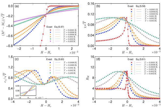
Figure s3: (color online) Scaling functions for magnetion (a), susceptibility (b), specific heat (c), Wilson ratio (d). Analytical results Eq. (S.56), Eq. (S.57), Eq. (S.59), Eq. (S.60) (lines) agree with numerical solutions of the TBA equations (S.4). These thermodynamical properties at different temperatures intersect at the critical point that reads off the critical exponents, see the main text.

Energy gap. At zero temperature, the antiferromagnetic Heisenbeg spin chain has a phase transition from a magnetized ground state to a ferromagnetic phase transition when the magnetic field excess the saturation magnetic field $H_{s}$. In the ferromagnetic phase an energy gap leads to spin wave quasiparticles with a gapped dispersion. The energy gap is obtained from the TBA equations at $T\to 0$, namely

$$\varepsilon_{1}\left(0\right)=H-4J=\Delta_{g},$$ (S.61)

where $H\geq 4J$. At low temperature, the conditions $\Delta_{g}/T\gg 1$ always holds, then we expand the free energy (S.51), then we get

susceptibility and specific heat in terms of energy gap

$$\chi=-\frac{1}{2\sqrt{\pi JT}}\operatorname{Li}_{-\frac{1}{2}}\left(-e^{-\frac{\Delta_{g}}{T}}\right),$$ (S.62)

specific heat

$$c_{v}=\sqrt{\frac{T}{\pi J}}\left[-\frac{3}{8}\operatorname{Li}_{\frac{3}{2}}\left(-e^{-\frac{\Delta_{g}}{T}}\right)+\frac{1}{2}\left(-\frac{\Delta_{g}}{T}\right)\operatorname{Li}_{\frac{1}{2}}\left(-e^{-\frac{\Delta_{g}}{T}}\right)-\frac{1}{2}\left(-\frac{\Delta_{g}}{T}\right)^{2}\operatorname{Li}_{-\frac{1}{2}}\left(-e^{-\frac{\Delta_{g}}{T}}\right)\right].$$ (S.63)

Taking the limit $\lim_{\left|z\right|\rightarrow 0}\operatorname{Li}_{s}\left(z\right)=z$, the gap equation of susceptibility and specific heat can be written as

$$\chi = -\frac{1}{2\sqrt{\pi JT}}\left(-e^{-\frac{\Delta_{g}}{T}}\right)=\frac{1}{2\sqrt{\pi JT}}e^{-\frac{\Delta_{g}}{T}},$$ (S.64)

$$c_{v} = \sqrt{\frac{T}{\pi J}}\left[\frac{3}{8}+\frac{1}{2}\left(\frac{\Delta_{g}}{T}\right)+\frac{1}{2}\left(\frac{\Delta_{g}}{T}\right)^{2}\right]e^{-\frac{\Delta_{g}}{T}}.$$ (S.65)

It is obviously that the susceptibility and specific show an exponential decay with respect to the energy gap. This nature was directly seen from our numerical and experimental fitting in the main text.

VI. Numerical solution to the TBA equations.

The analytical expression of the dressed energy is extremely hard to derive except for some limit cases, see the above sections. Here we develop new numerical method to deal with finite temperature magnetic properties of the 1D Heisenberg chain. The TBA equations (S.4) consist of infinite number of coupled integral equations of $\varepsilon_{n}(\lambda)$. In fact, it is also very difficult to solve numerically these equations. We observe that $\varepsilon_{n}(\lambda)$ approaches to a constant for a large value of $\lambda$, i.e.

$$\varepsilon_{n}(\infty)=T\text{ln}\Big{[}\Big{(}\frac{\text{sinh}[(n+1)H/(2T)]}{\text{sinh}[H/(2T)]}\Big{)}^{2}-1\Big{]}.$$ (S.66)

Moreover, $|\varepsilon_{n}(\lambda)-\varepsilon_{n}(\infty)|$ decreases with increasing the string length $n$. Thus we can take such advances to evaluate the quantity $\Delta\varepsilon_{n}^{\pm}(\lambda)=\varepsilon_{n}^{\pm}(\lambda)-\varepsilon_{n}^{\pm}(\infty)$. In order to achieve this goal, we rewrite the TBA equations (S.4) as

$$\Delta\varepsilon_{n}^{+}(\lambda)=-2\pi Ja_{n}(\lambda)-\sum_{m=1}^{n_{\rm c}}A_{m,n}\ast\Delta\varepsilon_{n}^{-}(\lambda)-\sum_{m=n_{\rm c}+1}^{\infty}A_{m,n}\ast\Delta\varepsilon_{n}^{-}(\lambda).$$ (S.67)

We choose the cut-off string number $n_{c}$ large enough such that $\sum_{m=n_{\rm c}+1}^{\infty}A_{m,n}\ast\Delta\varepsilon_{n}^{-}(\lambda)$ is negligiably small. Then we are capable of performing numerical calculation on the dressed energies and the thermodynamic quantities.

For the dressed energy is given by

$$f=\frac{H}{2}-2J\ln 2-T\ln[\cosh(\frac{H}{2T})]+\sum_{n=1}^{n_{\rm c}}g_{n}+\sum_{n=n_{\rm c}+1}^{\infty}g_{n},$$ (S.69)

$$g_{n}=\int{\rm d\lambda}a_{n}(\lambda)\Delta\varepsilon_{n}^{-}(\lambda).$$

Here we find that $g_{n}$ decays in a power law with respect to the string length $n$

$$g_{n}|_{n\gg 1}\propto n^{-a}$$ (S.70)

with a constant exponent $a$. For example, if we take $k_{B}T/J\approx 0.2$ and $g\mu_{B}H/J\approx 0$, we see $a\approx 3$. The value of $a$ increases with respect to the magnetic field $H$. We observe that $g\mu_{B}H/J\approx 2$, then $a\approx 10$. This suggests that even at the zero magnetic field limit, we still can solve the TBA equations numerically.

In a actual numerical process, we use $|(g_{n+1}-g_{n})/g_{1}|<d$ to estimate the errors, where $d$ is the accuracy. For example, we can estimate the string length cut-off $n_{c}$ by setting up an accuracy $d=10^{-6}$, see Fig.1 in the main text. The plateaux feature indicates that for a certain interval of $H$, there exists a cut-off $n_{c}$ which gives a high accurate numerical result with a given accuracy $d$. When the magnetic field $H$ is very small, higher length strings are needed in the numerical calculation. For an absence of the magnetic field, the contributions from high length spin strings should be taken account. In our numerical calculation, the major contributions $\sum_{n=1}^{\infty}\varepsilon_{n}^{-}(\infty)=\frac{H}{2}-2J\ln 2-T\ln[\cosh(\frac{H}{2T})]$ has been already considered analytically in the above equations. We only need to calculate $\Delta\varepsilon_{n}^{-}(\lambda)$ accurately. Upon the accuracy $d=10^{-6}$, we find that $n_{\rm c}=11$ is enough to maintain such an accuracy. In particular, we would like to emphasize that near the critical point $H_{s}$, we found that the length-1 string is accurate enough to capture the thermodynamical and magnetic properties of the spin chain in the vicinity of the critical point $H_{s}$.

References

(1)C. N. Yang, and C. P. Yang, Phys. Rev. 150, 321 (1966); Phys. Rev. 150, 327 (1966); Phys. Rev. 151, 258 (1966).
(2)L. D. Faddeev and L. A. Takhtajan, Phys. Lett. A 85, 375 (1981).
(3)F. D. M. Haldane, Phys. Rev. Lett. 47, 1840 (1981).
(4)A. Affleck, Phys. Rev. Lett. 56, 2763 (1986).
(5)M. Takahashi, Thermodynamics of One-Dimensional Solvable Models, (Cambridge University Press, Cambridge, 1999).
(6)Y. Wang, W.-L. Yang, J. Cao, K. Shi, Off-Diagonal Bethe Ansatz for Exactly Solvable Models, (Springer-Verlag Berlin Heidelberg 2015).
(7)D. C. Johnston et al., Phys. Rev. B 61, 9558 (2000).
(8)D. A. Tennant et al., Phys. Rev. B 52, 13368 (1995).
(9)B. Lake et al., 4, 329 (2005).
(10)M. Mourigal et al., Nat. Phys. 9, 435 (2013).
(11)B. Lake et al., Phys. Rev. Lett. 111, 137205 (2013).
(12)A. Zheludev et al., Phys. Rev. Lett. 100, 157204 (2008).
(13)M. B. Stone et al., Phys. Rev. Lett. 91, 037205 (2003).
(14)I. Affleck, Phys. Rev. Lett. 56, 746 (1986).
(15)J. Cardy, Nucl. Phys. B 270, 186 (1986).
(16)T. Giamarchi Quantum Physics in one dimension (Oxford University Press, Oxford, 2004).
(18)C. N. Yang, and C. P. Yang, J. Math. Phys. (N.Y.) 10, 1115 (1969).
(19)A. Sommerfeld, Z. Phys. 47, 1 (1928).
(20) K. G. Wilson, Rev. Mod. Phys. 47, 773 (1975).
(21)Y. Kono et al.,
Phys. Rev. Lett. 114, 037202 (2015).
(22)V. R. Shaginyan et al., Ann. Phys. (Berlin) 528, 483 (2016).
(23)H. A. Bethe, Z. Phys. 71, 205 (1931).
(24) See supplementary material.
(25)M. Karbach and G. Müller, Phys. Rev. B 62, 14871 (2000).
(26)M. Karbach, D. Biegel and G. Müller, Phys. Rev. B 66, 054405 (2002).
(27) J.-S. Caux, R. Hagemans, and J.-M. Maillet, J. Stat.
Mech. P09003 (2005).
(28)J.-S. Caux and R. Hagemans, J. Stat. Mech. P12013 (2006).
(29)A. Klauser, J. Mosset and J.-S. Caux, J. Stat. Mech. P03012 (2012).
(30)S. Lukyanov, Nucl. Phys. B 522, 533 (1998).
(31)S. Eggert, I. Affleck and M. Takahashi, Phys. Rev. Lett. 73, 332 (1994).
(32)J. C. Bonner and M. E. Fisher, Phys. Rev. 135, A640 (1964).
(33)L. Mezincescu and R. I. Nepomechie, Quantum groups, integrable models and statistical systems, eds. J. LeTourneux and L. Vinet, World Scientific Singapore (1993) pp 168-191;
L. Mezincescu et al., Nucl. Phys. B 406, 681
(1993).
(34)Y. Maeda, C. Hotta and M. Oshikawa, Phys. Rev. Lett. 99, 057205 (2007).
(35)Ch. Rüegg et al., Phys. Rev. Lett. 101, 247202 (2008).
(36) K. Ninios et al., 108, 097201 (2012).
(37) X. -W. Guan et al., Phys. Rev. Lett. 111, 130401 (2013).
(38)Y.-C. Yu and Y.-C. Chen, H.-Q. Lin, R. A. Roemer, and X.-W. Guan, Phys. Rev. B 94, 195129 (2016).
(39)Z. Saghafi et al., J. Mag. Mag. Mat. 398, 183 (2016).
(40)M. Klanjsek et al., Phys. Rev. Lett. 101, 137207 (2008).
(41)B. Thielemann et al., Phys. Rev. Lett. 102, 107204 (2009).
(42) P. R. Hammar et al., Phys. Rev. B 59, 1008 (1999).