Transport coefficients of a hot QCD medium and their relative significance in heavy-ion collisions

Abstract

The main focus of this article is to obtain various transport coefficients for a hot QCD medium that is produced while colliding two heavy nuclei ultra-relativistically. As the hot QCD medium follows dissipative hydrodynamics while undergoing space-time evolution, the knowledge of the transport coefficients such as thermal conductivity, electrical conductivity, shear and bulk viscosities are essential to understand the underlying physics there. The approach adopted here is semi-classical transport theory. The determination of all these transport coefficients requires knowledge of the medium away from equilibrium. In this context, we setup the linearized transport equation employing the Chapman-Enskog technique from kinetic theory of many particle system with a collision term that includes the binary collisions of quarks/antiquarks and gluons. In order to include the effects of a strongly interacting, thermal medium, a quasi-particle description of realistic hot QCD equation of state has been employed through the equilibrium modeling of the momentum distributions of gluons and quarks with non-trivial dispersion relations while extending the model for finite but small quark chemical potential. The effective coupling for strong interaction has been redefined following the charge renormalization under the scheme of the quasiparticle model. The consolidated effects on transport coefficients are seen to have significant impact on their temperature dependence. The relative significances of momentum and heat transfer as well as charge diffusion processes in hot QCD have been investigated by studying the ratios of the respective transport coefficients.

Keywords: Transport coefficients; Quark-gluon-plasma; Effective quasi-particle model; Electro-magnetic responses; Hot QCD equation of state

PACS: 12.38.Mh,  13.40.-f,  05.20.Dd,  25.75.-q

1 Introduction

The sub-nucleonic world of partonic substructures (quarks and gluons) have been studied with greater precision in last few decades, by exploring a deconfined state of the nuclear matter at relativistically energetic heavy-ion collider experiments. The experimental facilities at Relativistic Heavy Ion Collider (RHIC), BNL and Large Hadron Collider (LHC), CERN, have provided a fortune of data, which helped in revealing the thermodynamic and transport properties of the created medium after equilibration. A closer inspection on the experimental observables such as transverse momentum spectra and collective flows of charged hadrons or electromagnetic probes, reveals that their quantitative estimates should involve critical dependence upon the transport parameters of the system. This serves as a strong motivation for the quantitative study of the transport coefficients of this exotic medium (Quark-Gluon-Plasma (QGP)) that is created while colliding two heavy-ions such as Au-Au or Pb-Pb ultrarelativistically, along with a detailed study of their temperature dependences. The transport coefficients under investigation are, the shear and bulk viscosities ($\eta$ and $\zeta$) , electrical conductivity ($\sigma_{el}$) and thermal conductivity ($\lambda$) of the QGP medium. Besides providing information about the dissipation and electromagnetic (EM) responses of the medium, these transport parameters give relevant insights about the nature of interaction and non-equilibrium dynamics of the system as well. Earlier predictions of charged hadron elliptic flow from RHIC STAR and their theoretical explanations using dissipative hydrodynamics Luzum first provide the experimental evidence of existence of the transport processes in the QGP. More recently, a number of ALICE results have re confirmed the relevance of transport processes ALICE1 ; ALICE2 ; ALICE3 ; ALICE4 ; ALICE5 ; ALICE-JHEP . In particular in the context of the signal properties of charged hadrons and thermally produced particles (photons and dileptons), electromagnetic responses of the QGP medium also observed to play vital role which have been explored in Hirano ; Kharzeev1 ; Kharzeev2 ; Skokov ; Toneev ; Voloshin ; Zahed , in the due course of understanding the QGP medium.

The present article aims to estimate the temperature dependence of $\eta$, $\zeta$, $\lambda$ and $\sigma_{el}$ for a hot QCD medium/QGP created in heavy-ion collisions, including the effect of a finite quark chemical potential $\mu_{q}$. To explore the relative importance of these transport parameters and associated physical transport processes, their ratios in the form of known laws of known numbers in the literature have been investigated. The analysis has been done with semi-classical transport theory adopting Chapman-Enskog approach for many particle systems. The basic approach of determining the transport coefficients in kinetic theory is pursued by comparing the macroscopic and microscopic definitions of thermodynamic flows, as a results of which the particle interactions enter in the expressions of transport coefficients as dynamical inputs. Hence kinetic theory offers a unique scheme, that bridges between the microscopic events of particle interactions to its macroscopic effects (transport phenomena) on the thermodynamic system. In order to initiate the analysis and setup the appropriate transport equation, the very first requirement is the knowledge of local equilibrium momentum distributions of the gluonic and quark degrees of freedom that constitute the QGP. To that end, the modeling of equilibrium momentum distributions of gluons and quarks/antiquarks at vanishing and non-vanishing quark chemical potentials is needed to be done in a way that a realistic equation of state (EOS) for the QGP (such as lattice QCD EOS) could be mimicked. This has been done by adopting a recently introduced effective quasi-particle model by Chandra and Ravishankar Chandra_quasi1 ; Chandra_quasi2 where the hot QCD medium effects, present in the equations of state (EOSs) have been mapped to the equilibrium momentum distributions of quasiquarks and quasigluons containing temperature dependent quark and gluon effective fugacities. The modified thermodynamic quantities along with the non-trivial dispersion relation and the effective coupling of the strong interaction within the scope of the quasiparticle model, are observed to influence the temperature dependence of the transport parameters and the ratios significantly. It could be safely inferred that, the hot QCD medium effects, of a strongly correlated QGP liquid, introduced through the quasiparticle model, are being reflected in the temperature dependence of the estimated transport coefficients.

In order to quantify the energy-momentum dissipation during the space-time evolution of the system, shear and bulk viscous coefficients are needed to be estimated. The velocity gradient between the adjacent fluid layers results in the distortion of momentum distribution within the fluid elements, which gives rise to viscous forces. The viscous coefficients provide a measure of how the microscopic interactions within the system restore back the momentum distribution from skewed to isotropic. The thermal dissipation, occurring due to temperature gradient over the spatial separations of fluid, is described in terms of thermal conductivity for a system with conserved baryon current density. Besides the dissipative properties, one needs to investigate the electromagnetic (EM) responses in the QGP system, since a considerably strong EM field ($eB\sim m_{\pi}^{2}$) is being generated in the early stages of heavy ion collisions. In order to quantify the impact of the fields on electromagnetically charged QGP, the electrical conductivity plays quite useful role. It gives a measure of the electric current being induced in the response of the early stage electric field. In the strongly correlated systems like non-relativistic ultracold atomic Fermi gases or strongly coupled Bose fluids (in particular liquid helium), and for the QGP medium, the specific shear viscosity ($\eta/s$) is observed to have small values exhibiting near perfect fluidity of the system Schafer1 ; Schafer2 . The value of shear viscosity has been constrained by its ratio over system’s entropy density ($\eta/s$) by a lower bound $1/4\pi$, following the uncertainty principle and substantiated using anti-de Sitter space/conformal-field-theory (AdS/CFT) correspondence ADSCFT . The agreement of hydrodynamic description with the experimental data in Luzum also confirms this small value ($\eta/s=2/4\pi$) of shear viscous coefficient, which appears to be consistent with the values extracted directly from experiments Gavin and lattice simulations Nakamura as well. The magnitude of bulk viscosity, $\zeta$ is found to be quite small as compared to the shear viscosity, $\eta$, due to which early viscous hydrodynamic simulations ignored bulk viscosity for simplicity Heinz . Although it vanishes for a conformal fluid or massless QGP on the classical level, quantum effects break the conformal symmetry of QCD and generate a nonzero bulk viscosity even in the massless QGP phase, as recently shown by the lattice results Meyer in the $SU(3)$ pure gauge theory. Following the general argument that QCD to hadron gas transition is a crossover, $\eta/s$ shows a minimum near $T_{c}$, the critical temperature, close to the lower bound Csernai ; Lacey , whereas the bulk viscosity to entropy density ratio $\zeta/s$ shows large values around $T_{c}$ Karsch ; Pratt . Finally at FAIR energies and in the low-energy runs at RHIC, where the baryon chemical potential will be significant, thermal conductivity ($\lambda$) is expected to play important roles in the hydrodynamic evolution of the system. In Kapusta , the thermal conductivity is shown to diverge at the critical point and used to study the impact of hydrodynamic fluctuations on experimental observables. As a consequence of the strong electromagnetic field generated in the early stages of heavy ion collisions, the produced matter, after thermalization involves a non negligible electrical conductivity $\sigma_{el}$. In Deng , nontrivial time dependence of the electromagnetic fields is observed to be sensitive to this finite electrical conductivity. In Zakharov , the electromagnetic responses in the plasma fireball is demonstrated in the presence of a realistic $\sigma_{el}$, demanding a finite value of electrical conductivity in the QGP system. The relative behavior of these transport parameters leads to a comparative measure between different thermodynamic dissipations and electromagnetic responses. The mutual ratios between $\eta$, $\lambda$ and $\sigma_{el}$ can reflect the competition between momentum transport, heat transport and charge transport in the medium respectively, indicating different physical laws that will be elaborated in next section.

As already mentioned the physical laws connecting different transport coefficients provide a comparative study between the various collective behavior of the system under consideration. We start with the Wiedemann-Franz law which states that the thermal conductivity of a system is proportional to its electrical conductivity times the bulk temperature ($T$) of the system, such that $\lambda/(\sigma_{el}T)$ is a constant of temperature. The ratio is known as Lorentz number, which for most of the system including metals is independent of temperature depending only on the fundamental constants. In Ref. Crossno , a break-down of Wiedemann-Franz law has been reported for electron-hole plasma in graphene, indicating the signature of a strongly coupled Dirac fluid. In the same context, it is interesting to look into the behavior of this law in the strongly interacting QGP medium as well. Next, we focus on the relative behavior of viscous and thermal dissipation. From ADS/CFT studies of strongly coupled thermal gauge theories in the framework of the gauge-gravity duality, a value of the ratio between shear viscosity and thermal conductivity has been reported Son1 providing an analogue of the Wiedemann-Franz law between momentum transport and heat transport. For a system with finite chemical potential $\mu$, the ratio states $\frac{\lambda\mu^{2}}{\eta T_{H}}=8\pi^{2}$, where $T_{H}$ is the Hawking temperature. It is more customary to express the relative importance of kinematic viscosity or shear viscosity and thermal conductivity, in a dimensionless ratio called Prandtl number ($Pr$), given by $Pr=\eta c_{p}/\rho\lambda$, where $c_{p}$ is the specific heat at constant pressure of the system and $\rho$ is mass density of the system. In non-relativistic conformal holographic fluid this number is estimated to be $Pr=1$, from ADS/CFT computations Son2 . In Braby the Prandtl number is estimated to be $Pr=2/3$ for a dilute atomic Fermi gas, which agrees with the classical gas result. Finally, we mention about the relative behavior between shear viscosity and electrical conductivity which characterizes the relative importance of momentum diffusion and charge diffusion in a electromagnetically charged system that undergoes dissipation. We can specify this comparison by observing the ratio of two dimensionless quantities, $(\eta/s)/(\sigma/T)$. Since the electromagnetic responses are mostly carried by the charged components of the system, i.e, by the quarks in a strongly interacting QGP (although the diffusion flow of quarks and gluons are constrained to be coupled with each other, so that the gluon interaction rate in effect enters in the expression of electrical conductivity), whereas both quarks and gluons participate in momentum transport, the shear viscosity should dominate over the electrical conductivity as predicted by Greco , for strongly interacting QGP system. These physical laws and the associated ratios of transport parameters, providing useful informations about the dynamics and relative responses about the system, is instructive to relook for the QGP system, which is one of the major motivation of this work.

In order to provide the spectrum of the theoretical estimations of these transport quantities, we need to review the state of the art developments in recent literature. Turning out to be an useful signature of the phase transition occurring in the medium created in heavy ion collisions, the estimations of shear and bulk viscous coefficients have emerged as celebrated topics for quite some time both below and above the QCD transition temperature $T_{c}$. Above $T_{c}$ in the QGP sector, there are a number of estimations of the viscosities employing the transport theory approach utilizing kinetic theory of a many particle system Danielewicz ; Baym ; Thoma ; Heiselberg ; Hosoya ; AMY1 ; AMY2 ; Chen1 ; Chen2 ; Toneev-viscosity ; Greiner1 ; Greiner2 ; Schaefer-viscosity ; Jeon-Yaffe . Under the application of Kubo formalism the QGP viscosities have also been obtained by evaluating the correlation functions using linear response theory in Jeon ; Hosoya-Sakagami ; Carrington ; Basagoiti ; Moore . Describing the in medium constituent quark interactions under the scheme of Nambu-Jona-Lasinio(NJL) model, both the shear and bulk viscous coefficients have been estimated in Sasaki ; Deb ; Ghosh1 ; Ghosh2 . The quasiparticle approach, introduced in order to describe the hot QCD medium, has been employed to estimate the viscosities as well Plumari ; Chandra1 ; Chandra2 . The temperature dependence of $\eta$ and $\zeta$ have been constrained from hydrodynamic simulations and by comparing with the experimental data in Denicol ; Ryu ; Hirano2 . The molecular dynamics simulations have been employed in Shuryak to extract the shear viscosity to entropy density ratio for a strongly coupled QGP. Below the transition temperature, i.e, in the confined hadronic regime also a number of estimates of viscous coefficients are available Gavin-hadron ; Prakash ; NoronhaHostler ; Itakura ; Chen-hadron ; Davesne ; Dobado1 ; Dobado2 ; Dobado3 ; Dobado4 ; Dobado5 ; Buballa ; Albright ; Lang ; Wiranata ; Moore-hadron ; Moroz ; Chakraborty ; Pal ; Mitra1 ; Mitra2 ; Mitra3 . For quite a few times the viscous coefficients are being analyzed from holographic predictions as well. These viscous parameters are studied in great detail in a number of recent ADS/CFT based literature employing holographic QCD models Sachin ; Policastro ; Cremonini1 ; Cremonini2 ; Cremonini3 ; Cremonini4 ; Li ; Buchel . In comparison to the estimations of viscosities, the study of thermal conductivity has received much less attention in the current scenario. However a few estimated of $\lambda$ are available both in partonic and hadronic areas Gavin-hadron ; Prakash ; Davesne ; Greif ; Marty ; Nam ; Dobado-conductivity ; Nicola1 ; Nicola2 ; Mitra4 . Electrical conductivity, turning out to be an effective signature of electromagnetic responses in strongly interacting systems, has attained a lot of interest recently. In the strongly coupled QGP, the relativistic transport theory, dynamical quasiparticle model (DQPM) and the maximum entropy method (MEM), has found a number of applications to estimate the value and temperature dependence of $\sigma_{el}$ Greco ; Greiner-econd ; Greco-econd ; Cassing1 ; Cassing2 ; Qin ; Patra ; Mitra-Chandra . From the soft photon spectrum in heavy-ion collisions $\sigma_{el}$ has been extracted in Yin . Quite a considerable number of estimations of $\sigma_{el}$ are available from Lattice QCD computations as well Amato ; Aarts1 ; Aarts2 ; Gupta1 ; Brandt1 ; Brandt2 ; Ding ; Francis . In hadronic sector the contributions from Fraile ; Denicol-econd are prior to mention. Finally a number of holographic estimations have been proposed for both thermal and electrical conductivities in Finazzo ; Huot ; Sachin-cond1 ; Sachin-cond2 ; Sachin-cond3 ; Bu . A detailed comparison of the various transport coefficients obtained in the present work to the above mentioned existing interesting works will be presented in the later part of the manuscript.

The manuscript is organized as follows. Section 2, includes the formal developments of the transport theory, containing the Quasiparticle description of hot QCD medium, the evaluation and temperature behavior of thermal relaxation times of quarks and gluons within the medium and the detailed estimations of the transport coefficients in different subsections. The physical laws concerning the ratios of different transport coefficients have been discussed in Section 3. The obtained results have been discussed in Section 4. Finally in Section 5, the article has been summarized with providing possible outlooks of the work.

2 Formalism: Transport theory

Determination of transport coefficients for a hot QCD system needs modeling of the system away from equilibrium. Their determination can be done within two equivalent approaches, viz., the correlator technique in QCD using Green-Kubo formula, and the semiclassical transport theory (Chapman-Enskog or Grad’s 14 method). The present analysis is done following the latter approach. To initiate the formalism, an appropriate modeling of the equilibrium, isotropic momentum distributions of gluons and quark-antiquarks in the hot QCD medium at vanishing or non-vanishing baryon density (whatever be the case), is required to be provided. This could be systematically done by adopting an effective modeling of the hot QCD medium effects, encoded in the interacting QCD/QGP equations of state. To that end, the well accepted effective fugacity quasi-particle proposed by Chandra and Ravishankar  Chandra_quasi1 ; Chandra_quasi2 ; Chandra_quasi3 (EQPM) serves the current purpose which has been discussed below. The quasi-particle modeling of the system properties is followed by the estimations of the essential ingredients such as thermal relaxation times of interacting partons and other related quantities that are necessary while determining various transport coefficients under consideration here. Finally the complete formalism for extracting the transport coefficients is presented with all the required mathematical details below.

2.1 Effective modeling of momentum distributions of gluons and matter sector

The QCD medium at high temperature can conveniently be realized in terms of its effective quasi-particle degrees of freedom, viz., the quasi-gluons and quasi-quarks/antiquarks with non-trivial dispersion relations. There have been several quasi-particle models, proposed over the last few decades, to describe the hot QCD equations of state in terms of non-interacting or weakly interacting effective gluons and effective quarks and anti-quarks. The effective mass models Peshier1 ; Peshier2 ; Peshier3 ; Bannur1 ; Bannur2 ; Bannur3 ; Rebhan ; Thaler ; Szabo , the effective mass models with Polyakov loop DElia1 ; DElia2 ; Castorina1 ; Castorina2 ; Alba , describe the medium effects in terms of effective thermal mass or effective coupling in the medium. In these models, thermodynamic consistency condition is needed to be handled carefully, sometimes by introducing a few additional temperature dependence parameters. Another set of these models include, the NJL (Nambu Jona Lasinio) and the PNJL (Polyakov loop extended Nambu Jona Lasinio) based effective models Dumitru ; Fukushima ; SKGhosh ; Abuki . The EQPM which has been employed here, is described below in details.

2.1.1 The EQPM and its extension to finite quark chemical potential

The EQPM models the hot QCD medium effects in terms of effective quasi-partons (quasi-gluons, quasi-quarks/antiquarks). The main idea is to map the hot QCD medium effects present in the hot QCD EOSs either computed within improved perturbative QCD (pQCD) or lattice QCD simulations, into the effective equilibrium distribution functions for the quasi-partons. The EQPM for the QCD EOS at $O(g^{5})$ (EOS1) and $O(g^{6}\ln(1/g)+\delta)$ (EOS2) along with a recent (2+1)-flavor lattice QCD EOS (LEOS)  Cheng1 at physical quark masses, have been exploited in the present manuscript. Note that, there are more recent lattice results with the improved hot QCD actions and refined lattices Bazavov ; Cheng2 ; Borsanyi1 ; Borsanyi2 , for which, we need to re look the model with specific set of lattice data (specifically to define the effective gluonic degrees of freedom). Therefore, we will stick to the set of lattice data utilized in the model described in Ref. Chandra_quasi2 and leave the issue for further investigations in near future.

In either of these EOSs, form of the quasi-parton equilibrium distribution functions, $f_{eq}\equiv\{f_{g},f_{q,\bar{q}}\}$ (describing the strong interaction effects in terms of effective fugacities $z_{g,q}$) can be written as,

$$f_{g/q}=\frac{z_{g/q}\exp[-\beta E_{p}]}{\bigg{(}1\mp z_{g/q}\exp[-\beta E_{p}]\bigg{)}}$$ (1)

where $E_{p}=|\vec{p}|$ for the gluons and $\sqrt{|\vec{p}|^{2}+m_{q}^{2}}$ for the quarks/antiquarks ($m_{q}$ denotes the mass of the quarks). The parameter, $\beta=T^{-1}$ denotes inverse of the temperature, $\nu_{g}=2(N_{c}^{2}-1)$ denotes the gluonic degrees of freedom and $\nu_{q}=\nu_{\bar{q}}=2N_{c}N_{f}$, are the quark-antiquark degrees of freedom for $SU(N_{c})$ with $N_{f}$ number of flavors. Since the model is valid in the deconfined phase of QCD (beyond $T_{c}$), therefore, the mass of the light quarks can be neglected while comparing it with the temperature. Noteworthily, the EOS1 which is fully perturbative, is proposed by Arnold and Zhai Arnold-Zhai1 ; Arnold-Zhai2 and Zhai and Kastening Zhai-Karstening and the EOS2 which is at $O(g^{6}\ln(1/g)+\delta)$ is determined by Kajantie et al. Kajantie-Laine while incorporating contributions from non-perturbative scales such as $gT$ and $g^{2}T$. In the case of vanishing baryon density, $f_{q}\equiv f_{\bar{q}}$.

It is important to note that these effective fugacities, $z_{g/q}$ are not merely temperature dependent parameters that encode the hot QCD medium effects; they lead to non-trivial dispersion relation both in the gluonic and quark sectors as,

$$\omega_{g/q}=E_{p}+T^{2}\partial_{T}ln(z_{g/q}),$$ (2)

where $\omega_{g,q}$ denote the quasi-gluon and quasi-quark dispersions (single particle energy) respectively. The second term in the right-hand side of Eq.(2), encodes the effects from collective excitations of the quasi-partons.

The extension of the model to finite baryon/quark chemical potential is quite straightforward. This could be done by introducing the quark-chemical potentials ($\mu_{q}$) in the momentum distributions in the matter sector as:

$$f_{q/\bar{q}}=\frac{z_{q}\exp[-\beta(E_{p}\mp\mu_{q})]}{\bigg{(}1+z_{q}\exp[-\beta(E_{p}\mp\mu_{q})]\bigg{)}}$$ (3)

It is important to note that the temperature dependence of effective fugacities, $z_{g},z_{q}$ are set while implementing the EOS1, EOS2 and LEOS in terms of EQPM. In other words, while extending the EQPM for finite but small ($\mu_{q}/T<<1$) baryon densities, the same expressions for $z_{g}$ and $z_{q}$ have employed so that one can get the correct limit in case where $\mu_{q}=0$. The effective fugacities, $z_{g},z_{q}$ are not related with any conserved number current in the hot QCD medium. They have been merely introduced to encode the hot QCD medium effects in the EQPM. The physical interpretation of $z_{g}$ and $z_{q}$ emerges from the above mentioned non-trivial dispersion relations. The modified part of the energy dispersions in Eq. (2) leads to the trace anomaly (interaction measure) in hot QCD and takes care of the thermodynamic consistency condition. It is straightforward to compute, gluon and quark number densities and all the thermodynamic quantities such as energy density, entropy, enthalpy etc. by realizing the hot QCD medium in terms of an effective Grand canonical system Chandra_quasi1 ; Chandra_quasi2 . Furthermore, these effective fugacities lead to a very simple interpretation of hot QCD medium effects in terms of an effective Virial expansion. Note that $z_{g,q}$ scales with $T/T_{c}$, where $T_{c}$ is the QCD transition temperature. For the current analysis $T_{c}$ has been taken to be $170$ MeV. All the relevant thermodynamic quantities such as energy density, number density, pressure, entropy density, speed of sound etc. could straightforwardly be obtained in terms of $f_{g}$, $f_{q,\bar{q}}$ following their basic definitions. The detailed evaluation of these quantities at finite ($\mu_{q}$) are mentioned in the Appendix-B. The EQPM has recently been extended to non-extensive statistical systems keeping in view that the dense hadronic or QCD matter is generally produced in a nonextensive environment where the usual Boltzmann-Gibbs statistics is questionable and so the Tsallis statistics is being applied Wilk1 ; Tsallis .

2.1.2 Charge renormalization and effective coupling at finite $T$ and $\mu_{q}$

In contrast to the effective mass models where the effective mass is motivated from the mass renormalization in the hot QCD medium, the EQPM is based on the charge renormalization in high temperature QCD. This could be realized by computing the expression for the Debye mass in the medium following its definition that is derived in semi-classical transport theory Kelly1 ; Kelly2 ; Litim ; Blaizot as,

$$m_{D}^{2}=4\pi\alpha_{s}(T,\mu_{q})\bigg{(}-2N_{c}\int\frac{d^{3}p}{(2\pi)^{3}}\partial_{p}f_{g}(\vec{p})-N_{f}\int\frac{d^{3}p}{(2\pi)^{3}}\partial_{p}(f_{q}(\vec{p})+f_{\bar{q}}(\vec{p}))\bigg{)}$$ (4)

where, $\alpha_{s}(T)$ is the QCD running coupling constant at finite temperature and chemical potential

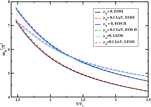
Figure 1: (Color online)Effective coupling constant using various EOSs as a function of $T/T_{c}$.

After performing the momentum integral and substituting the quasi-parton distribution function from Eq.(1) to Eq.(4), we are left with the expression of Debye mass within the scheme of EQPM model with finite quark chemical potential, upto the order $O(\tilde{\mu_{q}}^{2})$ (since $\tilde{\mu_{q}}^{2}<<1$),

$$m_{D}^{2}=4\pi\alpha_{s}(T,\mu_{q})T^{2}\bigg{\{}\bigg{(}\frac{2N_{c}}{\pi^{2}}\textrm{PolyLog}[2,z_{g}]-\frac{2N_{f}}{\pi^{2}}\textrm{PolyLog}[2,-z_{q}]\bigg{)}+{\tilde{\mu_{q}}^{2}}\frac{N_{f}}{\pi^{2}}\frac{z_{q}}{1+z_{q}}\bigg{\}}$$ (5)

The Debye mass here reduces to the leading order HTL expression in the limit $z_{g,q}\rightarrow 1$ (ideal EoS: non-interacting ultra relativistic quarks and gluons),

$$m_{D}^{2}(\textrm{HTL})=4\pi\alpha_{s}(T,\mu_{q})\ T^{2}\bigg{\{}(\frac{N_{c}}{3}+\frac{N_{f}}{6})+{\tilde{\mu_{q}}^{2}}\frac{N_{f}}{2\pi^{2}}\bigg{\}}~{}.$$ (6)

From Eq.(5) and (6), the effective coupling can be defined as:

$$\alpha_{eff}(T,\mu_{q})=\alpha_{s}(T,\mu_{q})\times\frac{\big{\{}\frac{2N_{c}}{\pi^{2}}\textrm{PolyLog}[2,z_{g}]-\frac{2N_{f}}{\pi^{2}}\textrm{PolyLog}[2,-z_{q}]\big{\}}+\tilde{\mu_{q}}^{2}\big{\{}\frac{N_{f}}{\pi^{2}}\frac{z_{q}}{1+z_{q}}\big{\}}}{\big{\{}\frac{N_{c}}{3}+\frac{N_{f}}{6}\big{\}}+\tilde{\mu_{q}}^{2}\big{\{}\frac{N_{f}}{2\pi^{2}}\big{\}}}~{}.$$ (7)

The behavior of the ratio $m_{D}^{2}/T^{2}$ as a function of temperature ($T/T_{c}$) for various EOSs and finite $\mu_{q}$ is depicted in Fig. 1. As expected, the finite but small $\mu_{q}$ effects are quite visible at lower temperatures, which are merging with the zero quark chemical potential cases at higher temperatures. This is seen to be valid for all the three EOSs considered here. The medium effects (thermal) manifested through the temperature dependent $z_{g,q}$, play the crucial role in modulating the quantity $m_{D}^{2}/T^{2}$ as a function of temperature.

There are only three free functions ($z_{g}$, $z_{q}$, and $\tilde{\mu}_{q}$) in the EQPM employed here. The first two, depend on the chosen EOS. In the case of EOS1 and EOS2 employed in the present case, these functions are obtained in Chandra_quasi1 and are continuous functions of $T/T_{c}$. On the other hand, for LEOS they are defined in terms of eight parameters obtained in Ref. Chandra_quasi2 (See Table I of Ref. Chandra_quasi2 ). The quantity $\tilde{\mu_{q}}$ is chosen to be $0.0$ and $0.1$ GeV throughout our analysis. In addition, the effective coupling mentioned above depends on the QCD running coupling constant $g(T,\mu_{q})=\sqrt{4\pi\alpha_{s}}$, that explicitly depends upon how we fix the QCD renormalization scale at finite temperature and $\mu_{q}$, and up to what order we define $g(T,\mu_{q})$. Henceforth, these are the only quantities that are needed to be supplied throughout the analysis here.

Notably, the EQPM employed here has been remarkably useful in understanding the bulk and the transport properties of the QGP in heavy-ion collisions Chandra_eta1 ; Chandra_eta2 ; Chandra_dilep1 ; Chandra_dilep2 ; Chandra_hq1 ; Chandra_hq2 ; Chandra_hq3 . Before, the formalism for estimations of thermal relaxation times of the constituent gluons and quarks are being discussed, it is important to highlight the utility of quasi-particle models in the context of understanding the bulk and transport properties of the hot QCD/QGP medium created out of the heavy-ion collisions. As already mentioned transport parameters of the QGP have estimated employing various quasiparticle models in Plumari ; Chandra1 ; Chandra2 ; Albright ; Chandra_eta1 ; Chandra_eta2 ; Bluhm . Note that Ref. Bluhm offered the estimation of $\eta$ and $\zeta$ for pure gluon plasma employing the effective mass quasi-particle model. On the other hand, Refs. Chandra1 ; Chandra2 ; Chandra_eta1 ; Chandra_eta2 , reported their estimation for both gluonic as well as matter sector. Refs. Chakraborty ; Albright , presented the quasi-particle estimations of $\eta$ and $\zeta$ in hadronic sector. The thermal conductivity has also been studied, in addition to the viscosity parameters Albright , within the effective mass model at finite baryon density.

2.2 Thermal Relaxation times

As mentioned earlier, the microscopic interactions between the constituents of the system, provide the dynamical inputs for different transport coefficients. Here, it is done by introducing the thermal relaxation times of the partons, which in turn, introduce the transport cross sections to the expressions of the transport coefficients.

In order to define the thermal relaxation times for quasi quarks/anti quarks and gluons, we start with the relativistic transport equation of the momentum distribution functions of the constituent partons in an out of equilibrium, multicomponent system that describes the binary elastic process $p_{k}+p_{l}\rightarrow p^{\prime}_{k}+p^{\prime}_{l}$,

$$p_{k}\partial_{\mu}f_{k}=\sum_{l=1}^{N}C_{kl}[f_{k},f_{l}],~{}~{}~{}~{}~{}~{}~{}~{}~{}~{}~{}~{}~{}~{}~{}~{}[k=1,2,..........N]~{}.$$ (8)

Here $f_{k}$ is the single particle distribution function for the $k^{th}$ species, that depends upon the particle 4-momentum $p_{k}$ and 4-space-time coordinates $x$. Here, the right hand side of Eq.(8) denotes the collision term that quantifies the rate of change of $f_{k}$. For each $l$, $C_{kl}[f_{k},f_{l}]$ defines the collision contribution due to the scattering of $k^{th}$ particle with $l^{th}$ one given in the following manner  AMY1 ,

$$C_{kl}[f_{k},f_{l}]=\frac{1}{2}\frac{\nu_{l}}{2}\int d\Gamma_{p_{l}}d\Gamma_{p^{\prime}_{k}}d\Gamma_{p^{\prime}_{l}}(2\pi)^{4}\delta^{4}(p_{k}+p_{l}-p^{\prime}_{k}-p^{\prime}_{l})\langle|M_{k+l\rightarrow k+l}|^{2}\rangle$$

$$[f_{k}(p^{\prime}_{k})f_{l}(p^{\prime}_{l})\{1\pm f_{k}(p_{k})\}\{1\pm f_{l}(p_{l})\}-f_{k}(p_{k})f_{l}(p_{l})\{1\pm f_{k}(p^{\prime}_{k})\}\{1\pm f_{l}(p^{\prime}_{l})\}]~{}.$$ (9)

The phase space factor is given by the notation $d\Gamma_{p_{i}}=\frac{d^{3}\vec{p_{i}}}{(2\pi)^{3}2\omega_{i}}$, as $\omega_{k}$ is the energy of the scattered particle (of the $k^{th}$ species). The overall $\frac{1}{2}$ factor appears due to the symmetry in order to compensate for the double counting of final states that occurs by interchanging $p^{\prime}_{k}$ and $p^{\prime}_{l}$. $\nu_{l}$ is the degeneracy of $2^{nd}$ particle that belongs to $l^{th}$ species.

In the next section it will be shown that upto the next to leading order, the out of equilibrium distribution function is constructed as follows,

$$f_{k}=f_{k}^{0}+\delta f_{k}=f_{k}^{0}+f_{k}^{0}(1\pm f_{k}^{0})\phi_{k}~{},$$ (10)

where the non-equilibrium part $\delta f_{k}$ of the distribution function is quantified by the deviation function $\phi_{k}$. The distribution functions of the quasi partons at local thermal equilibrium is given by Eq.(1).

In the next section, we will see that the simplest method of linearizing the transport equation (8)is to replace the collision term by the rate of change of the distribution function over the thermal relaxation time $\tau_{k}$ which is needed by the out of equilibrium distribution function to restore its equilibrium value, such that the transport equation becomes,

$$\frac{df_{k}}{dt}=-\frac{\delta f_{k}}{\tau_{k}}=-\frac{(f_{k}-f_{k}^{0})}{\tau_{k}}~{}.$$ (11)

Consequently the collision term becomes,

$$C_{kl}[f_{k},f_{l}]=-\omega_{k}\frac{\delta f_{k}}{\tau_{k}}=-\omega_{k}\frac{f_{k}^{0}(1\pm f_{k}^{0})\phi_{k}}{\tau_{k}}~{}.$$ (12)

Putting (10) into the right hand side of (9) by assuming the distribution functions of the particles other than the scattered one are very much close to equilibrium and comparing with (12), the relaxation time finally becomes as the inverse of the reaction rate $\Gamma_{k}$ of the respective processes  Zhang ,

$$\tau_{k}^{-1}\equiv\Gamma_{k}= \frac{\nu_{l}}{2}\frac{1}{2\omega_{k}}\int d\Gamma_{p_{l}}d\Gamma_{p^{\prime}_{k}}d\Gamma_{p^{\prime}_{l}}(2\pi)^{4}\delta^{4}(p_{k}+p_{l}-p^{\prime}_{k}-p^{\prime}_{l})$$ (13)

$$\langle|M_{k+l\rightarrow k+l}|^{2}\rangle\frac{f_{l}^{0}(1\pm f_{k}^{{}^{\prime}0})(1\pm f_{l}^{{}^{\prime}0})}{(1\pm f_{k}^{0})}~{}.$$

Clearly the distribution function of final state particles are given by primed notation.

Simplifying $\tau_{k}$ utilizing the $\delta$-function we finally obtain its expression in the center of momentum frame of particle interaction as,

$$\tau_{k}^{-1}=\Gamma_{k}=\nu_{l}\int\frac{d^{3}\vec{p_{l}}}{(2\pi)^{3}}d(\cos\theta)\frac{d\sigma}{d(\cos\theta)}\frac{f_{l}^{0}(1\pm f_{k}^{{}^{\prime}0})(1\pm f_{l}^{{}^{\prime}0})}{(1\pm f_{k}^{0})}~{},$$ (14)

where $\theta$ is the scattering angle in the center of momentum frame and $\sigma$ is the interaction cross section for the respective scattering processes. Now in terms of the Mandelstam variables $s,t$ and $u$ the expression for $\tau_{k}$ can be reduced simply as,

$$\tau_{k}^{-1}=\Gamma_{k}=\nu_{l}\int\frac{d^{3}\vec{p_{l}}}{(2\pi)^{3}}dt\frac{d\sigma}{dt}\frac{f_{l}^{0}(1\pm f_{k}^{{}^{\prime}0})(1\pm f_{l}^{{}^{\prime}0})}{(1\pm f_{k}^{0})}~{}.$$ (15)

The differential cross section relates the scattering amplitudes as $\frac{d\sigma}{dt}=\frac{\langle|M|^{2}\rangle}{16\pi s^{2}}$. The QCD scattering amplitudes for $2\rightarrow 2$ binary, elastic processes are taken from  Combridge , that are averaged over the spin and color degrees of freedom of the initial states and summed over the final states. The inelastic processes like $q\overline{q}\rightarrow gg$, have been ignored in the present case, because they do not have a forward peak in the differential cross section and thus their contributions will presumably be small compared to the elastic ones.

Now in order to take into account the small-angle scattering scenario that results into divergent contributions from $t$-channel diagrams of QCD interactions, a transport weight factor $(1-\cos\theta)=\frac{2tu}{s^{2}}$ has been introduced in the interaction rate  Hosoya . Furthermore considering the momentum transfer $q=|\vec{p_{k}}-\vec{p^{\prime}_{k}}|=|\vec{p_{l}}-\vec{p^{\prime}_{l}}|$ is not too large we can make following assumptions, $f_{k}^{0}\cong f_{k}^{{}^{\prime}0}$ and $f_{l}^{0}\cong f_{l}^{{}^{\prime}0}$  Thoma1 to finally obtain,

$$\tau_{k}^{-1}=\Gamma_{k}=\nu_{l}\int\frac{d^{3}\vec{p_{l}}}{(2\pi)^{3}}f_{l}^{0}(1\pm f_{l}^{0})\int dt\frac{d\sigma}{dt}\frac{2tu}{s^{2}}~{}.$$ (16)

This additional transport factor changes the infrared and ultraviolet behavior of the interaction rate quite significantly. Due to inclusion of this term all the higher order divergences reduce to simple logarithmic singularities which can be simply handled by putting a small angle cut-off in the integration limit. In the integration involving $t$-channel diagrams from where the infrared logarithmic singularity appears, the limit of integration is restricted from $-s$ to $-k^{2}$ in order to avoid those divergent results using the cut-off $k^{2}=g^{2}T^{2}$ as infrared regulator. Here $g^{2}=4\pi\alpha_{s}$ with $\alpha_{s}$ being the coupling constant of strong interaction as already mentioned in Section 1.

Now in the QGP medium the quark and gluon interaction rates result from the following interactions respectively,

$$\Gamma_{g}=\Gamma_{gg}+\Gamma_{gq}+\Gamma_{g\overline{q}}~{},~{}~{}~{}~{}~{}~{}\Gamma_{q}=\Gamma_{qg}+\Gamma_{qq}+\Gamma_{q\overline{q}}~{},~{}~{}~{}~{}~{}~{}\Gamma_{\overline{q}}=\Gamma_{\overline{q}g}+\Gamma_{\overline{q}q}+\Gamma_{\overline{q}\overline{q}}~{}$$ (17)

where $\Gamma_{kl}$, is the interaction rate of $k^{th}$ particle due to scattering with the $l^{th}$ one.

Finally after pursuing the angular integration in (16) we are left with the thermal relaxation times of the quark, antiquark and gluon components in a QGP system in the following way,

$$\tau_{g}^{-1}= \{\nu_{g}\int\frac{d^{3}\vec{p_{g}}}{(2\pi)^{3}}f_{g}^{0}(1+f_{g}^{0})\}[\frac{9g^{4}}{16\pi\langle s\rangle_{gg}}\{ln\frac{\langle s\rangle_{gg}}{k^{2}}-1.267\}]$$

$$+ \{\nu_{q}\int\frac{d^{3}\vec{p_{q}}}{(2\pi)^{3}}f_{q}^{0}(1-f_{q}^{0})\}[\frac{g^{4}}{4\pi\langle s\rangle_{gq}}\{ln\frac{\langle s\rangle_{gq}}{k^{2}}-1.287\}]$$

$$+ \{\nu_{\overline{q}}\int\frac{d^{3}\vec{p_{\overline{q}}}}{(2\pi)^{3}}f_{\overline{q}}^{0}(1-f_{\overline{q}}^{0})\}[\frac{g^{4}}{4\pi\langle s\rangle_{g\overline{q}}}\{ln\frac{\langle s\rangle_{g\overline{q}}}{k^{2}}-1.287\}],$$ (18)

$$\tau_{q}^{-1}= \{\nu_{g}\int\frac{d^{3}\vec{p_{g}}}{(2\pi)^{3}}f_{g}^{0}(1+f_{g}^{0})\}[\frac{g^{4}}{4\pi\langle s\rangle_{qg}}\{ln\frac{\langle s\rangle_{qg}}{k^{2}}-1.287\}]$$

$$+ \{\nu_{q}\int\frac{d^{3}\vec{p_{q}}}{(2\pi)^{3}}f_{q}^{0}(1-f_{q}^{0})\}[\frac{g^{4}}{9\pi\langle s\rangle_{qq}}\{ln\frac{\langle s\rangle_{qq}}{k^{2}}-1.417\}]$$

$$+ \{\nu_{\overline{q}}\int\frac{d^{3}\vec{p_{\overline{q}}}}{(2\pi)^{3}}f_{\overline{q}}^{0}(1-f_{\overline{q}}^{0})\}[\frac{g^{4}}{9\pi\langle s\rangle_{q\overline{q}}}\{ln\frac{\langle s\rangle_{q\overline{q}}}{k^{2}}-1.417\}]~{},$$ (19)

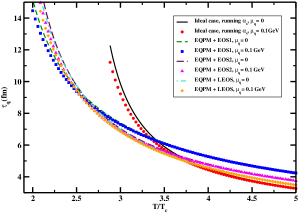
Figure 2: Thermal relaxation times for gluons and quarks using various EOSs as a function of $T/T_{c}$ at fixed $\tilde{\mu}_{q}$.

$$\tau_{\overline{q}}^{-1}= \{\nu_{g}\int\frac{d^{3}\vec{p_{g}}}{(2\pi)^{3}}f_{g}^{0}(1+f_{g}^{0})\}[\frac{g^{4}}{4\pi\langle s\rangle_{\overline{q}g}}\{ln\frac{\langle s\rangle_{\overline{q}g}}{k^{2}}-1.287\}]$$

$$+ \{\nu_{q}\int\frac{d^{3}\vec{p_{q}}}{(2\pi)^{3}}f_{q}^{0}(1-f_{q}^{0})\}[\frac{g^{4}}{9\pi\langle s\rangle_{\overline{q}q}}\{ln\frac{\langle s\rangle_{\overline{q}q}}{k^{2}}-1.417\}]$$

$$+ \{\nu_{\overline{q}}\int\frac{d^{3}\vec{p_{\overline{q}}}}{(2\pi)^{3}}f_{\overline{q}}^{0}(1-f_{\overline{q}}^{0})\}[\frac{g^{4}}{9\pi\langle s\rangle_{\overline{q}\overline{q}}}\{ln\frac{\langle s\rangle_{\overline{q}\overline{q}}}{k^{2}}-1.417\}]~{},$$ (20)

where $\langle s\rangle_{kl}=2\langle p_{k}\rangle\langle p_{l}\rangle$ is the thermal average value of $s$ with $\langle p_{k}\rangle=\frac{\int\frac{d^{3}\vec{p_{k}}}{(2\pi)^{3}}|\vec{p_{k}}|f_{k}^{0}}{\int\frac{d^{3}\vec{p_{k}}}{(2\pi)^{3}}f_{k}^{0}}$. Clearly in order to account for a hot QCD medium the quasiparticle effects must be invoked in the expressions of these thermal relaxation times obtained far. As discussed in Section 2.1, the distribution functions of quarks and gluons and the coupling $g$ will carry the quasiparticle descriptions accordingly. Since the cut-off parameter $k$ also depends upon $g$ and the thermal average of $s$ includes $f^{0}_{g,q,\overline{q}}$, they will reflect the hot QCD equation of state effect as well. Following the definition of equilibrium distribution function of quarks and gluons from Eq.(1), within the quasiparticle framework, the thermal averages of gluon and quark momenta respectively are obtained as,

$$\langle p_{g}\rangle= 3T\frac{\textrm{PolyLog}[4,z_{g}]}{\textrm{PolyLog}[3,z_{g}]}~{},$$ (21)

$$\langle p_{q}\rangle= 3T\frac{\textrm{PolyLog}[4,-z_{q}]+\tilde{\mu_{q}}\textrm{PolyLog}[3,-z_{q}]+\frac{(\tilde{\mu_{q}})^{2}}{2}\textrm{PolyLog}[2,-z_{q}]}{\textrm{PolyLog}[3,-z_{q}]+\tilde{\mu_{q}}\textrm{PolyLog}[3,-z_{q}]-\frac{(\tilde{\mu_{q}})^{2}}{2}ln(1+z_{q})}~{},$$ (22)

$$\langle p_{\overline{q}}\rangle= 3T\frac{\textrm{PolyLog}[4,-z_{q}]-\tilde{\mu_{q}}\textrm{PolyLog}[3,-z_{q}]+\frac{(\tilde{\mu_{q}})^{2}}{2}\textrm{PolyLog}[2,-z_{q}]}{\textrm{PolyLog}[3,-z_{q}]-\tilde{\mu_{q}}\textrm{PolyLog}[3,-z_{q}]-\frac{(\tilde{\mu_{q}})^{2}}{2}ln(1+z_{q})}~{}.$$ (23)

The degeneracy factors used, are $\nu_{g}=2\times 8=16$, $\nu_{q}=\nu_{\overline{q}}=2\times N_{c}\times N_{f}$, with $N_{f}$ and $N_{c}$ are the quark number of flavors and colors respectively. From the above analysis, it turned out that the thermal relaxation times at a particular $\mu_{q}$ follows the form given as,

$$\tau_{q/\overline{q},g}^{-1}\sim T\alpha_{s}^{2}ln\bigg{\{}\frac{1}{\alpha_{s}}\bigg{\}}~{}.$$ (24)

In Fig.(2), the temperature dependence of the thermal relaxation times of quasi gluons and quarks, obtained from Eq.(18) and (19) respectively, have been plotted as a function of $T/T_{c}$. The temperature dependence of $\tau$ for both the gluonic and quark components, is observed to exhibit the obvious decreasing trend with increasing temperature, revealing that the enhanced interaction rates at higher temperatures make the thermal quarks and gluons restore down their equilibrium faster. We observe at a particular temperature, $\tau_{q}$ is quantitatively little greater than $\tau_{g}$, indicating stronger interaction rates of the gluonic part. The order of magnitude of the relaxation times and the fact that $\tau_{q}$ is larger than $\tau_{g}$, agree with the work given in Baym .

In the present case the $\tau_{g}$ and $\tau_{q}$ have been estimated for three different EOSs (EOS1, EOS2, LEOS) within the scope of EQPM along with ideal EOS with running coupling and also for two different quark chemical potentials ($\mu_{q}=0,\ 0.1$GeV). As noticed earlier in the case of QCD coupling, here also the finite quark chemical potential effects are only significant at lower temperatures which almost diminishes at higher temperature regions. The large values of $\tau_{g}$ and $\tau_{q}$ for the ideal case at lower temperature mostly result from the higher values of running $\alpha_{s}(T,\mu_{q})(\sim 0.4)$ compare to the $\alpha_{eff}(T,\mu_{q})(\sim 0.3)$, contributing through the logarithmic term. However at higher temperatures, the plots of $\tau$’s including the quasiparticle equation of state effects are merging with the ideal ones, as at those temperature regions the quasiparticle properties almost behave like that of the free particles. Three different set of plots with EQPM calculations are clearly showing the distinct effects of separate EOSs. In each set, the small but finite effects of non-zero $\mu_{q}$ is observed at lower temperatures, which is more predominant in the plots of $\tau_{q}$ for obvious reasons. So we conclude that first the logarithmic term in Eq.(24) is playing here the key role in determining the temperature behavior of $\tau$’s and secondly different EOSs describing the interacting medium through various models (pQCD or Lattice) and the non-zero $\mu_{q}$ is providing considerable effects on it.

2.3 Estimation of transport coefficients in Chapman-Enskog method

The basic scheme of determining the transport coefficients of a many particle system resides in comparing the macroscopic and microscopic definition of thermodynamic flows. The description of irreversible phenomena taking place in non equilibrium systems is characterized by two kinds of concepts : the thermodynamic forces and thermodynamic flows. The first ones create spatial non-uniformities of the macroscopic thermodynamic state variables where the later tend to restore back the equilibration situation by wiping out these non-uniformities. Phenomenologically, one finds to a good approximation that these fluxes are linearly related to the thermodynamic forces where the proportionality constants are termed as transport coefficients. As a consequence the irreversible part of the energy momentum tensor and the heat flow can be expressed in a linear law, directly proportional to the corresponding thermodynamic forces which is respectively the velocity gradient and temperature gradient of the system. From the second law of thermodynamics, it is known that the restoration of equilibrium is achieved by the processes which involve increasing entropy. From these criteria the viscous pressure tensor and the irreversible heat flow of the system are expressed by the following equations respectively  Degroot ; Weinberg ,

$$\Pi^{\mu\nu}= 2\eta\langle\partial^{\mu}u^{\nu}\rangle+\zeta\Delta^{\mu\nu}\partial\cdot u~{},$$ (25)

$$I^{\mu}= \lambda(\partial_{\sigma}T-TDu_{\sigma})\Delta^{\mu\sigma}~{},$$ (26)

where the constant of proportionalities $\eta,\zeta$ and $\lambda$ are referred to as the transport coefficients. The notation used are explained below. The hydrodynamic velocity $u^{\mu}$ defined in a comoving frame as $u^{\mu}=(1,0,0,0)$. $\Delta^{\mu\nu}=g^{\mu\nu}-u^{\mu}u^{\nu}$ is the projection operator, with $g^{\mu\nu}=(1,-1,-1,-1)$ as the metric of the system. $\langle t^{\mu\nu}\rangle\equiv[\frac{1}{2}(\Delta^{\mu\alpha}\Delta^{\nu\beta}+\Delta^{\nu\alpha}\Delta^{\mu\beta})-\frac{1}{3}\Delta^{\mu\nu}\Delta^{\alpha\beta}]t_{\alpha\beta}$ indicates a space-like symmetric and traceless form of the tensor $t^{\mu\nu}$.

The alternative definition of thermodynamic fluxes at microscopic level involves an integral over the product of non-equilibrium or collisional part of the distribution function of particles and an irreducible tensor of the quantity which is being transported. Following this prescription the viscous pressure tensor and the irreversible heat flow can be given by the following integral equations,

$$\Pi^{\mu\nu}= \sum_{k=1}^{N}\nu_{k}\int\frac{d^{3}\vec{p}_{k}}{(2\pi)^{3}p_{k}^{0}}\Delta^{\mu}_{\sigma}\Delta^{\nu}_{\tau}p_{k}^{\sigma}p_{k}^{\tau}\delta f_{k},$$ (27)

$$I^{\mu}= \sum_{k=1}^{N}\nu_{k}\int\frac{d^{3}\vec{p}_{k}}{(2\pi)^{3}p_{k}^{0}}(p_{k}.u-h_{k})p_{k}^{\sigma}\Delta^{\mu}_{\sigma}\delta f_{k}.$$ (28)

Here $p_{k}$ and $h_{k}$ are the particle 4-momenta and enthalpy per particle respectively. So, comparing the set of equations in (25,26) and (27,28), the values of $\eta$, $\zeta$ and $\lambda$ can be estimated as a function of the particle distribution deviation $\delta f_{k}$.

For a system with electrically charged constituents, under the influence of an external electric field the induced current density relates with the field itself by a linear relation via electrical conductivity ($\sigma_{el}$) as,

$$J^{\mu}=\sigma_{el}E^{\mu}~{}.$$ (29)

In microscopic definition the current density of such a system is given by Greif-Thesis ,

$$J^{\mu}(x)=\sum_{k=1}^{N}q_{k}I_{k}^{\mu}=\sum_{k=1}^{N-1}(q_{k}-q_{N})I_{k}^{\mu}~{},$$ (30)

where $q_{k}$ is the electric charge associated with the $k^{th}$ species. The diffusion flow $I^{\mu}_{a}$ for a non equilibrium relativistic system including all reactive processes into account, is given by,

$$I_{a}^{\mu}= \sum_{k=1}^{N}q_{ak}I_{k},~{}~{}~{}~{}~{}~{}~{}~{}~{}~{}~{}~{}~{}~{}~{}~{}[a=1,2,..........N^{\prime}]$$ (31)

$$= \sum_{k=1}^{N}q_{ak}\{N_{k}^{\mu}-x_{k}N^{\mu}\}~{}.$$ (32)

Here $a$ stands for the index of conserved quantum number and $q_{ak}$ is the $a^{th}$ conserved quantum number associated with $k^{th}$ component. $N_{k}^{\mu}(x)=\sum_{k=1}^{N}N_{k}^{\mu}(x)$ stands for the total particle 4-flow, where the particle 4-flow for the $k^{th}$ species in a multicomponent system is defined as, $N_{k}^{\mu}(x)=\int\frac{d^{3}\vec{p_{k}}}{(2\pi)^{3}p_{k}^{0}}p_{k}^{\mu}f_{k}(x,p_{k})$. $x_{k}=\frac{n_{k}}{n}$ is defined as the particle fraction corresponding to $k^{th}$ species with $n_{k}=\int\frac{d^{3}\vec{p_{k}}}{(2\pi)^{3}}f_{k}(x,p_{k})$ , and $n=\sum_{k=1}^{N}n_{k}(x)$, as the particle number density of $k^{th}$ species and total number density of the system respectively.

Putting Eq.(32) into Eq.(30), and comparing with Eq.(29) we can obtain $\sigma_{el}$ again as a function of the particle distribution deviation $\delta f_{k}$.

Observing that the transport coefficients depend upon $\delta f_{k}=f^{0}_{k}(1\pm f^{0}_{k})\phi_{k}$, we need to obtain a scheme to determine this quantity in an out of equilibrium thermodynamic system. We proceed by solving the relativistic transport equation (8), in a technique called Chapman-Enskog method from the kinetic theory of a multicomponent, many particle system. In Chapman-Enskog method the distribution function is expanded in a series in terms of a parameter. This parameter must be a small, dimensionless quantity in order to make the series asymptotic, such that leading order terms in the expansion must be significant as compared to the next to leading order ones. Before introducing a useful quantity that can be used as the expansion parameter, let us investigate the transport equation (8) again,

$$p^{\mu}_{k}\partial_{\mu}f_{k}=\sum_{l=1}^{N}C_{kl}[f_{k},f_{l}],~{}~{}~{}~{}~{}~{}~{}~{}~{}~{}~{}~{}~{}~{}~{}~{}[k=1,2,..........N]~{}.$$ (33)

The derivative on the left hand side of equation (33) is decomposed into a time-like and a space-like part as $\partial^{\mu}=u^{\mu}D+\nabla^{\mu}$, with the covariant time derivative $D=u^{\mu}\partial_{\mu}$ and the spatial gradient $\nabla_{\mu}=\Delta_{\mu\nu}\partial^{\nu}$. The resulting equation is obtained as,

$$p_{k}^{\mu}u_{\mu}Df_{k}+p_{k}^{\mu}\nabla_{\mu}f_{k}=\sum_{l=1}^{N}C_{kl}[f_{k},f_{l}].$$ (34)

We observe that the length scale associated with the collision term on the right hand side of the transport equation is the mean free path ($\lambda_{c}$) of the hydrodynamic system. The length scale associated with the terms on the left hand side of transport equation is the characteristic dimension for the spatial non-uniformities within the system, i.e, it is the typical length $L$ over which the macroscopic thermodynamic quantities within the system can vary appreciably. The dimensionless ratio $\lambda_{c}/L$ is called the Knudsen number and let us denote it by $\epsilon=\lambda_{c}/L$. The order of magnitude of the ratio of a typical term on the right hand side of transport equation to a typical term on the left hand side is the Knudsen number $\epsilon$ and due to this fact one can introduce $\epsilon$ (which must be small in the hydrodynamic regime where the deviation from equilibrium is small), as a dimensionless parameter in front of the left hand side of the transport equation depicted below to balance the magnitude of length scale of both sides of transport equation,

$$\epsilon\{p_{k}^{\mu}u_{\mu}Df_{k}+p_{k}^{\mu}\nabla_{\mu}f_{k}\}=\sum_{l=1}^{N}C_{kl}[f_{k},f_{l}].$$ (35)

Next, we present the expansion of the particle distribution function in a power series of $\epsilon$ in the following way,

$$f_{k}=\sum_{n=0}^{\infty}\epsilon^{n}f_{k}^{(n)}~{}.$$ (36)

In covariant notation, the time derivative over distribution function is expanded as follows,

$$Df_{k}=(Df_{k})^{0}+\epsilon(Df_{k})^{1}+\epsilon^{2}(Df_{k})^{2}+.............=\sum_{n=0}^{\infty}\epsilon^{n}(Df_{k})^{(n)}~{}.$$ (37)

where the term $(Df_{k})^{(n)}$ simply denotes $\partial f_{k}^{(n)}/\partial t$. Equations (36) and (37) helps to expand transport equation in terms of the non-uniformity parameter $\epsilon$. Substituting them into the transport equation (35) and equating the coefficients of equal power in $\epsilon$, we obtain the hierarchy of equations,

$$0=\sum_{k=1}^{N}C_{kl}[f_{k}^{(0)},f_{l}^{(0)}]~{},$$ (38)

$$p_{k}^{\mu}u_{\mu}(Df_{k})^{r-1}+p_{k}^{\mu}\nabla_{\mu}f_{k}^{r-1}=\sum_{s=0}^{r}\sum_{l=1}^{N}C_{kl}[f_{k}^{(s)},f_{l}^{(r-s)}],~{}~{}~{}~{}~{}~{}~{}~{}~{}~{}~{}r\geq 1~{}.$$ (39)

Equation (38) reveals nothing but the Boltzmann transport equation for a fluid in equilibrium where the collision term involving equilibrium distribution function vanishes. Equation (39) provides a hierarchy of equations where in the left hand side of the transport equation the derivatives appear on the lower order of distribution function, and the next order appear on the right hand side only under the collision term. If the $r$th order of distribution function is expressed as $f_{k}^{(r)}=f_{k}^{(0)}(1\pm f_{k}^{(0)})\phi^{(r)}$, then employing the principle of detailed balance $f_{k}^{(0)}(x,p_{k})f_{l}^{(0)}(x,p_{l})=f_{k}^{(0)}(x,p_{k}^{\prime})f_{l}^{(0)}(x,p^{\prime}_{l})$ we obtain,

$$C[f_{k}^{(0)},f_{l}^{(r)}]+C[f_{k}^{(r)},f_{l}^{(0)}]=-{{\cal L}_{kl}}[\phi_{k}^{(r)},\phi_{l}^{(r)}]~{}.$$ (40)

The unknown function $\phi_{k}^{(r)}$, which depends upon particle 4-momenta and fluid space-time co-ordinates, is needed to be determined. Here, we can see that the non-linear collision term is linearized under the function $\phi_{k}^{(r)}$ and the linearized collision operator is defined as,

$${\cal L}_{kl}[\phi_{k}^{(r)},\phi_{l}^{(r)}]= \frac{1}{2}\nu_{l}f_{k}^{(0)}(x,p_{k})\int d\Gamma_{p_{l}}\ d\Gamma_{p^{\prime}_{k}}\ d\Gamma_{p^{\prime}_{l}}f_{l}^{(0)}(x,p_{l})\{1+f_{k}^{(0)}(x,p^{\prime}_{k})\}\{1+f_{l}^{(0)}(x,p^{\prime}_{l})\}$$ (41)

$$[\phi^{(r)}_{k}(x,p_{k})+\phi^{(r)}_{l}(x,p_{l})-\phi^{(r)}_{k}(x,p^{\prime}_{k})-\phi^{(r)}_{l}(x,p^{\prime}_{l})]W(p_{k},p_{l}|p^{\prime}_{k},p^{\prime}_{l})~{}.$$

Here $W=\frac{1}{2}(2\pi)^{4}\delta^{4}(p_{k}+p_{l}-p^{\prime}_{k}-p^{\prime}_{l})\langle|M_{k+l\rightarrow k+l}|^{2}\rangle$ is the interaction cross sections for the corresponding dynamical processes. In this way the Chapman-Enskog hierarchy becomes,

$$p_{k}^{\mu}u_{\mu}(Df_{k})^{r-1}+p_{k}^{\mu}\nabla_{\mu}f_{k}^{(r-1)}-\sum_{s=1}^{r-1}\sum_{l=1}^{N}C_{kl}[f_{k}^{(s)},f_{l}^{(r-s)}]=-\sum_{l=1}^{N}{{\cal L}_{kl}}[\phi_{k}^{(r)},\phi_{l}^{(r)}]~{}.$$ (42)

From the foregoing discussion it follows that the first Chapman-Enskog approximation is determined by equation (42) for r=1

$$p_{k}^{\mu}u_{\mu}(Df_{k})^{0}+p_{k}^{\mu}\nabla_{\mu}f_{k}^{(0)}=-\sum_{l=1}^{N}{{\cal L}_{kl}}[\phi_{k}^{(1)},\phi_{l}^{(1)}]~{}.$$ (43)

In equation (43) the quantity $\phi_{k}^{(1)}$ is the measure of the deviation of the distribution function in the first approximation of Chapman-Enskog method from its equilibrium value and from here on we are restricting our estimations for $\phi_{k}^{(1)}$ only. Hence throughout this article this quantity has been simply denoted by $\phi_{k}$. So the next to leading order correction in the leading order equilibrium distribution function is,

$$\delta f_{k}=f_{k}^{(1)}=f_{k}^{(0)}(1\pm f_{k}^{(0)})\phi_{k}~{}.$$ (44)

From the above hierarchy of equations, it can be well understood that the Chapman-Enskog technique is an iterative method, where from the known lower order distribution function the unknown next order can be determined by successive approximation.

Here the linearization of the collision integral, by turning it into a linear integral operator with symmetric kernel, in terms of the deviation function $\phi_{k}$, in the right hand side of Eq.(43) is extremely essential. In general, the program of seeking solution of transport equation becomes non-trivial due to the non-linearity of the collision term. However if the state of the system is not considered to be too far from the equilibrium as in the present case, one may assume that a linearized form of the transport equation provides a reasonably accurate description of the non-linear phenomena. Now one of the conventional mathematical tool to treat the Integro-Differential equation containing the linearized collision term, is the variational approximation method, in which the deviation function is expanded in a polynomial series to any desired degrees of accuracy. However for a multicomponent system with $N$ number of independent particle species this polynomial method leads to expressing the transport coefficients in terms of a $N\times N$ matrix whose elements include the 4-particle phase space integrals containing the explicit interaction cross sections. This again becomes non-trivial to tackle along with the in medium corrections in the collective properties of a strongly interacting, thermal system. So in order to provide a solution without much loss in generality in the context of the situation concerned, we decide to proceed by treating the collision term in relaxation time approximation (RTA). In this method the collision term is replaced by the rate of change of the distribution function over the thermal relaxation times $\tau_{k}$ for particular species as discussed in section 2.2. Following the RTA scheme Eq.(43) finally reduces to,

$$p_{k}^{\mu}u_{\mu}(Df_{k})^{0}+p_{k}^{\mu}\nabla_{\mu}f_{k}^{0}=-\frac{\omega_{k}}{\tau_{k}}f_{k}^{0}(1\pm f_{k}^{0})\phi_{k}~{}.$$ (45)

In the presence of an external electromagnetic force, the left hand side of the relativistic transport equation includes also a covariant force term $q_{k}F^{\alpha\beta}p_{\beta}\frac{\partial f_{k}}{\partial p_{k}^{\alpha}}$, where $q_{k}$ is the electronic charge of the $k^{th}$ species particle and $F^{\mu\nu}=\{-u^{\mu}E^{\nu}+u^{\nu}E^{\mu}\}$ is the electromagnetic field tensor with electric field $E^{\mu}$, in the absence of any magnetic field in the medium. After incorporating this force term in to Eq.(45), we finally obtain the linearized transport equation under the Chapman-Enskog scheme as the following,

$$p_{k}^{\mu}u_{\mu}(Df_{k})^{0}+p_{k}^{\mu}\nabla_{\mu}f_{k}^{0}+\frac{1}{T}f_{k}^{0}(1\pm f_{k}^{0})q_{k}E_{\mu}p_{k}^{\mu}=-\frac{\omega_{k}}{\tau_{k}}f_{k}^{0}(1\pm f_{k}^{0})\phi_{k}~{}.$$ (46)

Now applying the definition of equilibration momentum distribution function of quasi quarks/anti-quarks and quasi gluons from Eq.(1) on the left hand side of Eq.(46) and exploiting a number of thermodynamic identities which are nothing but equilibrium thermodynamic evolution equations of macroscopic state variables of the system, following from certain conservation laws (discussed in Appendix-A), we are left with a number of thermodynamic forces with different tensorial ranks,

$$Q_{k}X+\langle p_{k}^{\nu}\rangle\{(p_{k}.u)-h_{k}\}X_{qk}+\langle p_{k}^{\nu}\rangle\sum_{a=1}^{N^{\prime}-1}(q_{ak}-x_{a})X_{a\nu}-\langle p_{k}^{\mu}p_{k}^{\nu}\rangle\langle X_{\mu\nu}\rangle=-\frac{T\omega_{k}}{\tau_{k}}\phi_{k}~{},$$ (47)

with,

$$X= \partial\cdot u~{},$$ (48)

$$X_{q\mu}= [\frac{\partial_{\mu}T}{T}-\frac{\partial_{\mu}P}{nh}]+[-\frac{1}{h}\sum_{k=1}^{N}x_{k}q_{k}E_{\mu}]~{},$$ (49)

$$X_{k\mu}= [(\partial_{\mu}\mu_{k})_{P,T}-\frac{h_{k}}{nh}\partial_{\mu}P]+[q_{k}-q_{N}-\frac{h_{k}-h_{N}}{h}\sum_{l=1}^{N}x_{l}q_{l}]E_{\mu}~{},$$ (50)

$$\langle X_{\mu\nu}\rangle= \langle\partial_{\mu}u_{\nu}\rangle=\frac{1}{2}\{\Delta_{\mu\alpha}\Delta_{\nu\beta}+\Delta_{\nu\alpha}\Delta_{\mu\beta}-\frac{2}{3}\Delta_{\mu\nu}\Delta_{\alpha\beta}\}\partial^{\alpha}u^{\beta}~{}.$$ (51)

Here $Q_{k}=\frac{1}{3}\{|\vec{p_{k}}|^{2}-3\omega_{k}^{2}c_{s}^{2}\}$, with $c_{s}$ is the velocity of sound propagation within the medium and, $(\partial_{\mu}\mu_{a})_{P,T}=\sum_{b=1}^{N^{\prime}-1}\{\frac{\partial\mu_{a}}{\partial x_{b}}\}_{P,T,\{x_{a}\}}\partial_{\mu}x_{b}$, with $x_{a}$ and $\mu_{a}$ are the particle fraction and chemical potential associated with $a^{th}$ quantum number respectively. Tensors of form $\langle p_{k}^{\mu}p_{k}^{\nu}\rangle=\frac{1}{2}\{\Delta^{\mu\alpha}\Delta^{\nu\beta}+\Delta^{\nu\alpha}\Delta^{\mu\beta}-\frac{2}{3}\Delta^{\mu\nu}\Delta^{\alpha\beta}\}(p_{k})_{\alpha}(p_{k})_{\beta}$, and $\langle p_{k}^{\mu}\rangle=\Delta^{\mu\nu}(p_{k})_{\nu}$, are called irreducible tensor of rank 2 and 1 respectively, where the rank 0 is simply a scalar. These tensors are irreducible with respect to the transformation group, consisting of those Lorentz transformations $\Lambda$, which leaves the time-like vector $u^{\mu}$ invariant ($\Lambda^{\mu}_{\nu}u^{\nu}=u^{\mu}$). The natural occurrence of these form of tensors in problems involving spherical symmetry and the fact that they can form a complete set of tensors with minimum number of members, have made their application quite convenient and advantageous in kinetic theory.

Now, we observe that different thermodynamic forces indicated by Eq.(48)-(51) involves different transport processes. $X$, expressing the trace part of velocity gradient is known as bulk viscous force. The quantity, $X_{q\mu}$ is related to the temperature gradient known as thermal driving force. $X_{k\mu}$ includes the spatial gradient over chemical potential that can be translated into the gradient over particle fraction (($\nabla^{\mu}\mu_{k})_{P,T}=\frac{T}{x_{k}}\nabla^{\mu}x_{k}$), and thus known as diffusion driving force. Finally $\langle X_{\mu\nu}\rangle$, containing the traceless part of velocity gradient is known as the shear viscous force. The respective viscous forces give rise to shear ($\eta$) and bulk ($\zeta$) viscous coefficient where as thermal driving force gives rise to thermal conductivity$\lambda$. We notice that, apart of the spatial gradients over thermodynamic quantities, the thermal driving force and the diffusion driving forces include finite contributions purely from the $E^{\mu}$, reflecting the response of the external electric field in the medium. So we can conclude that in the expressions of thermal and diffusion driving forces, terms proportional to electric field give rise to electrical conductivity ($\sigma_{el}$).

Now in order to be a solution of Eq.(47) the deviation function $\phi_{k}$ must be a linear combination of the thermodynamic forces in the following manner,

$$\phi_{k}=A_{k}X+B_{k}^{\mu}X_{q\mu}+\frac{1}{T}\sum_{a=1}^{N^{\prime}-1}B_{ak}^{\mu}X_{a\mu}-C_{k}^{\mu\nu}\langle X_{\mu\nu}\rangle~{},$$ (52)

where $A,B$ and $C$ are the unknown coefficients with appropriate tensorial ranks consistent with the thermodynamic forces, such that $\phi_{k}$ becomes a scalar, needed to be estimated from the transport equation itself. In order to do so, we put Eq.(52) on the right hand side of Eq.(47) and by the virtue of the fact that thermodynamic forces are independent of each other we finally obtain,

$$A_{k}= \frac{Q_{k}}{\{-\frac{T\omega_{k}}{\tau_{k}}\}}~{},$$ (53)

$$B_{k}^{\mu}= \langle p_{k}^{\mu}\rangle\frac{\omega_{k}-h_{k}}{\{-\frac{T\omega_{k}}{\tau_{k}}\}}~{},$$ (54)

$$B_{ak}^{\mu}= T\langle p_{k}^{\mu}\rangle\frac{q_{ak}-x_{a}}{\{-\frac{T\omega_{k}}{\tau_{k}}\}}~{},$$ (55)

$$C_{k}^{\mu\nu}= \frac{\langle p_{k}^{\mu}p_{k}^{\nu}\rangle}{\{-\frac{T\omega_{k}}{\tau_{k}}\}}~{}.$$ (56)

Utilizing the expressions rom Eq.(53)-(56) and putting the expression of $\phi_{k}$ from Eq.(52) into Eq.(44), we finally obtain the full expression of the deviation of the partonic distribution function $\delta f_{k}$. Now we are in a situation where by putting the expression of deviation of the distribution function into the microscopic definitions of thermodynamic fluxes and comparing them with the macroscopic definitions of the same, the transport coefficients can be estimated explicitly as discussed earlier. Here, we need to mention one crucial property of the irreducible tensor used so far. Due to isotropy and the relativistic invariance of the of the collision operator, it can be observed that the thermodynamic flows and forces of different tensorial rank do not couple, while they of equal rank do couple by via scalar coefficients. The inner product of two irreducible tensors of different ranks gives rise to zero, where with equal ranks they completely contract giving rise to scalar transport coefficients. This statement is famous as Curie’s principle in the framework of relativistic kinetic theory. It beautifully takes care of the fact, that only the relevant physical phenomena responsible for the deviation of particle’s momentum distribution from equilibrium, will be contributed to the respective thermodynamic flows. The next four sub sections will be contributed for the evaluation of the four different transport coefficients namely shear viscosity ($\eta$), bulk viscosity ($\zeta$), thermal conductivity ($\lambda$) and electrical conductivity ($\sigma_{el}$).

2.3.1 Shear viscosity

As discussed in the previous section, in order to estimate the viscous coefficients we need to compare the expressions of viscous pressure tensor from Eq.(25) and Eq.(27). It is convenient to split $\Pi^{\mu\nu}$ into a traceless part and a remainder such as,

$$\Pi^{\mu\nu}=\langle{\Pi}^{\mu\nu}\rangle+\Pi\Delta^{\mu\nu}~{}.$$ (57)

The viscous pressure $\Pi$ is defined as one third of the trace of the viscous pressure tensor,

$$\Pi=\sum_{k=1}^{N}\nu_{k}\frac{1}{3}\int\frac{d^{3}\vec{p}_{k}}{(2\pi)^{3}p_{k}^{0}}\Delta_{\mu\nu}p_{k}^{\mu}p_{k}^{\nu}\delta f_{k}~{}.$$ (58)

So the trace less part of viscous pressure tensor comes out to be,

$$\langle{\Pi}^{\mu\nu}\rangle=\Pi^{\mu\nu}-\Pi\Delta^{\mu\nu}=\sum_{k=1}^{N}\nu_{k}\int\frac{d^{3}\vec{p}}{(2\pi)^{3}p^{0}}\langle p^{\mu}p^{\nu}\rangle\delta f_{k}~{}.$$ (59)

Clearly Eq.(58) will give rise to bulk viscosity while Eq.(59) gives rise to shear viscosity. Putting the expression of $\delta f_{k}$, with the expression of $\phi_{k}$ from Eq.(52), into Eq.(59) and comparing with Eq.(25) we obtain the expression of shear viscosity as,

$$\eta=\sum_{k=1}^{N}\nu_{k}\frac{\tau_{k}}{15T}\int\frac{d^{3}\vec{p}_{k}}{(2\pi)^{3}}\frac{|\vec{p_{k}}|^{4}}{\omega^{2}_{k}}f_{k}^{0}(1\pm f_{k}^{0})~{}.$$ (60)

In the context of the current article, the shear viscosity for a strongly interacting QGP system is provided with the help of the thermal relaxation times of constituent partons from Eq.(18), (19) and (20), and the quasiparticle equilibrium distribution functions of the same under EQPM scheme from Eq.(1) as the following,

$$\eta= \nu_{q}\frac{\tau_{q}}{15T}\int\frac{d^{3}\vec{p}_{q}}{(2\pi)^{3}}\frac{|\vec{p_{q}}|^{4}}{\omega^{2}_{q}}f_{q}^{0}(1-f_{q}^{0})$$

$$+ \nu_{\overline{q}}\frac{\tau_{\overline{q}}}{15T}\int\frac{d^{3}\vec{p}_{\overline{q}}}{(2\pi)^{3}}\frac{|\vec{p_{\overline{q}}}|^{4}}{\omega^{2}_{\overline{q}}}f_{\overline{q}}^{0}(1-f_{\overline{q}}^{0})$$

$$+ \nu_{g}\frac{\tau_{g}}{15T}\int\frac{d^{3}\vec{p}_{g}}{(2\pi)^{3}}\frac{|\vec{p_{g}}|^{4}}{\omega^{2}_{g}}f_{g}^{0}(1+f_{g}^{0})~{}.$$ (61)

Here the quasiparticle energy per partons under the EQPM model can be derived from the dispersion relation given in Eq.(2) as,

$$\omega_{k}=|\vec{p_{k}}|[1+\{\frac{T}{|\vec{p_{k}}|}\}\{\frac{T}{T_{c}}\}\partial_{(\frac{T}{T_{c}})}\{lnz_{k}\}]~{}.$$ (62)

We have estimated $\eta$ from Eq.(61) in two ways. First an exact estimation of $\eta$ from Eq.(61) has been obtained using full numerical coding. Secondly we perform an analytical approximation of Eq.(61) in the following manner by investigating its level of accuracy. By analyzing the temperature dependence of effective fugacity parameter $z_{k}$, we have examined the second term on the right hand side of Eq.(62). For gluonic case, at $T/T_{c}=2.5$ we obtain from Eq.(62),

$$\omega_{g}=|\vec{p_{g}}|[1+0.094]~{}.$$ (63)

So the correction in $\omega_{k}$ due to the fugacity term is less than $10\%$. (Similar estimations can be shown for quark degrees of freedom as well.) So Eq.(63) can be conveniently expanded in a binomial series keeping upto only $2^{nd}$ order term. Following this prescription the $\frac{1}{\omega_{k}^{2}}$ term in the expression of $\eta$, can be reduced to,

$$\frac{1}{\omega_{k}^{2}}=\frac{1}{|\vec{p_{k}}|^{2}}-\frac{2}{|\vec{p_{k}}|^{3}}[T(\frac{T}{T_{c}})\partial_{(\frac{T}{T_{c}})}\{lnz_{k}\}]~{}.$$ (64)

Following Eq.(64), the expression of $\eta$, with the analytical approximation performed, becomes

$$\eta=\sum_{k=q,\overline{q},g}\nu_{k}\frac{\tau_{k}}{15T}[\int\frac{d^{3}\vec{p}_{k}}{(2\pi)^{3}}|\vec{p_{k}}|^{2}f_{k}^{0}(1\pm f_{k}^{0})-2\{T(\frac{T}{T_{c}})\partial_{(\frac{T}{T_{c}})}(lnz_{k})\}\int\frac{d^{3}\vec{p}_{k}}{(2\pi)^{3}}|\vec{p_{k}}|f_{k}^{0}(1\pm f_{k}^{0})]~{}.$$ (65)

The momentum integrations over the equilibrium quasiparticle distribution functions are analytically computable giving compact results in terms of PolyLog functions of the fugacity parameters of quasi-quarks and gluons,

$$\eta= \big{(}\frac{2T^{4}}{5\pi^{2}}\big{)}\nu_{g}\tau_{g}[2\textrm{Polylog}[4,z_{g}]-\{\big{(}\frac{T}{T_{c}}\big{)}\partial_{(\frac{T}{T_{c}})}(lnz_{g})\}\textrm{Polylog}[3,z_{g}]]$$

$$+ \big{(}\frac{2T^{4}}{5\pi^{2}}\big{)}\nu_{q}\tau_{q}[-2\{\textrm{Polylog}[4,-z_{q}]+\tilde{\mu_{q}}\textrm{Polylog}[3,-z_{q}]+\frac{{\tilde{\mu_{q}}}^{2}}{2}\textrm{Polylog}[2,-z_{q}]\}$$

$$+ \{\big{(}\frac{T}{T_{c}}\big{)}\partial_{(\frac{T}{T_{c}})}(lnz_{q})\}\{\textrm{Polylog}[3,-z_{q}]+\tilde{\mu_{q}}\textrm{Polylog}[2,-z_{q}]-\frac{{\tilde{\mu_{q}}}^{2}}{2}ln(1+z_{q})\}]$$

$$+ \big{(}\frac{2T^{4}}{5\pi^{2}}\big{)}\nu_{\overline{q}}\tau_{\overline{q}}[-2\{\textrm{Polylog}[4,-z_{q}]-\tilde{\mu_{q}}\textrm{Polylog}[3,-z_{q}]+\frac{{\tilde{\mu_{q}}}^{2}}{2}\textrm{Polylog}[2,-z_{q}]\}$$

$$+ \{\big{(}\frac{T}{T_{c}}\big{)}\partial_{(\frac{T}{T_{c}})}(lnz_{q})\}\{\textrm{Polylog}[3,-z_{q}]-\tilde{\mu_{q}}\textrm{Polylog}[2,-z_{q}]-\frac{{\tilde{\mu_{q}}}^{2}}{2}ln(1+z_{q})\}]$$

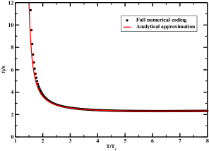
Figure 3: Shear viscosity to entropy ratio using various EOSs as a function of $T/T_{c}$ at fixed $\tilde{\mu}_{q}$.

In Fig.(3) the obtained shear viscosity over entropy density ratio (derived in Appendix-B) has been plotted as a function of $T/T_{c}$ . The first figure is showing the comparison between fully numerical estimation directly from Eq.(61) and the approximated analytical estimation from Eq.(LABEL:SV-10) of $\eta/s$ for $N_{f}=3$, with LEOS under EQPM scheme at $\mu_{q}=0.1$ GeV. The plot shows that the two curves are merely separable from each other above $T/T_{c}\sim 2~{}~{}(T\sim 300$MeV). So it can be clearly inferred that the analytical approximation performed in the estimation of $\eta$ is quite reliable in the temperature range we are interested currently. The right panel of the same figure exhibits the temperature dependence of $\eta/s$ estimated under the EQPM scheme using three separate EOSs mentioned in section (2.1) for zero and non-zero $\mu_{q}$. As predicted by other pQCD estimates, the value of $\eta/s$ is observed to be greater than the experimental extractions and ADS/CFT predictions which is $\sim 0.1$ (discussed later in details). Here the leading log term in thermal relaxation time inputs are majorly responsible for the enhanced value of $\eta/s$. Upto $T/T_{c}\sim 4$ the equation of state effects under EQPM are quite distinctly visible which is merging with the ideal ones in high temperature ranges. The non-zero $\mu_{q}$ effects are only slightly visible in lower temperatures which becomes negligible in high temperatures.

2.3.2 Bulk viscosity

The bulk viscous coefficients can be estimated in the same spirit as $\eta$ by comparing Eq.(58) and (25), and putting the expression of $\phi_{k}$ from Eq.(52) into $\delta f_{k}$,

$$\zeta=\sum_{k=q,\overline{q},g}\nu_{k}\frac{\tau_{k}}{9T}\int\frac{d^{3}\vec{p}_{k}}{(2\pi)^{3}}\frac{1}{\omega^{2}_{k}}\{p_{k}^{2}-3\omega_{k}^{2}c_{s}^{2}\}^{2}f_{k}^{0}(1\pm f_{k}^{0})~{}.$$ (67)

Under the analytical approximation mentioned in the earlier section Eq.(67) becomes,

$$\zeta =(1-3c_{s}^{2})^{2}\sum_{k=q,\overline{q},g}\nu_{k}\frac{\tau_{k}}{9T}\int\frac{d^{3}\vec{p}_{k}}{(2\pi)^{3}}|\vec{p_{k}}|^{2}f_{k}^{0}(1\pm f_{k}^{0})$$ (68)

$$-2(1-9c_{s}^{4})\sum_{k=q,\overline{q},g}\nu_{k}\frac{\tau_{k}}{9T}\big{\{}T\big{(}\frac{T}{T_{c}}\big{)}\partial_{(T/T_{c})}\{lnz_{k}\}\big{\}}\int\frac{d^{3}\vec{p}_{k}}{(2\pi)^{3}}|\vec{p_{k}}|f_{k}^{0}(1\pm f_{k}^{0})$$

$$+(1+3c_{s}^{2})^{2}\sum_{k=q,\overline{q},g}\nu_{k}\frac{\tau_{k}}{9T}\big{\{}T\big{(}\frac{T}{T_{c}}\big{)}\partial_{(T/T_{c})}\{lnz_{k}\}\big{\}}^{2}\int\frac{d^{3}\vec{p}_{k}}{(2\pi)^{3}}f_{k}^{0}(1\pm f_{k}^{0})~{}.$$

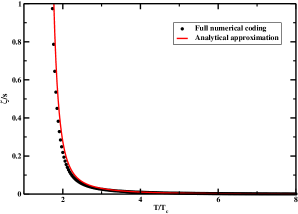
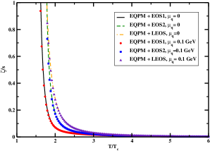
Figure 4: Bulk viscosity to entropy ratio using various EOSs as a function of $T/T_{c}$ at fixed $\tilde{\mu}_{q}$.

After performing the momentum integrals over separate partonic degrees of freedom, we obtain the consolidated expression of $\zeta$ in terms of the Polylog function over fugacity parameters in the following way,

$$\zeta =(1-3c_{s}^{2})^{2}\tau_{g}\nu_{g}(\frac{4T^{4}}{3\pi^{2}})\textrm{PolyLog}[4,z_{g}]$$

$$-(1-9c_{s}^{4})\tau_{g}\nu_{g}(\frac{2T^{4}}{3\pi^{2}})[(\frac{T}{T_{c}})\partial_{(\frac{T}{T_{c}})}(lnz_{g})]\textrm{PolyLog}[3,z_{g}]$$

$$+(1+3c_{s}^{2})^{2}\tau_{g}\nu_{g}(\frac{T^{4}}{9\pi^{2}})[(\frac{T}{T_{c}})\partial_{(\frac{T}{T_{c}})}(lnz_{g})]^{2}\textrm{PolyLog}[2,z_{g}]$$

$$+(1-3c_{s}^{2})^{2}\tau_{q}\nu_{q}(\frac{4T^{4}}{3\pi^{2}})[-\{\textrm{PolyLog}[4,-z_{q}]+\tilde{\mu_{q}}\textrm{Polylog}[3,-z_{q}]+\frac{{\tilde{\mu_{q}}}^{2}}{2}\textrm{Polylog}[2,-z_{q}]\}]$$

$$-(1-9c_{s}^{4})\tau_{q}\nu_{q}(\frac{2T^{4}}{3\pi^{2}})[(\frac{T}{T_{c}})\partial_{(\frac{T}{T_{c}})}(lnz_{q})][-\{\textrm{PolyLog}[3,-z_{q}]+\tilde{\mu_{q}}\textrm{Polylog}[2,-z_{q}]-\frac{{\tilde{\mu_{q}}}^{2}}{2}ln(1+z_{q})\}]$$

$$+(1+3c_{s}^{2})^{2}\tau_{q}\nu_{q}(\frac{T^{4}}{9\pi^{2}})[(\frac{T}{T_{c}})\partial_{(\frac{T}{T_{c}})}(lnz_{q})]^{2}[-\{\textrm{PolyLog}[2,-z_{q}]-\tilde{\mu_{q}}ln(1+z_{q})-\frac{{\tilde{\mu_{q}}}^{2}}{2}\frac{z_{q}}{1+z_{q}}\}]$$

$$+(1-3c_{s}^{2})^{2}\tau_{\overline{q}}\nu_{\overline{q}}(\frac{4T^{4}}{3\pi^{2}})[-\{\textrm{PolyLog}[4,-z_{q}]-\tilde{\mu_{q}}\textrm{Polylog}[3,-z_{q}]+\frac{{\tilde{\mu_{q}}}^{2}}{2}\textrm{Polylog}[2,-z_{q}]\}]$$

$$-(1-9c_{s}^{4})\tau_{\overline{q}}\nu_{\overline{q}}(\frac{2T^{4}}{3\pi^{2}})[(\frac{T}{T_{c}})\partial_{(\frac{T}{T_{c}})}(lnz_{q})][-\{\textrm{PolyLog}[3,-z_{q}]-\tilde{\mu_{q}}\textrm{Polylog}[2,-z_{q}]-\frac{{\tilde{\mu_{q}}}^{2}}{2}ln(1+z_{q})\}]$$

$$+(1+3c_{s}^{2})^{2}\tau_{\overline{q}}\nu_{\overline{q}}(\frac{T^{4}}{9\pi^{2}})[(\frac{T}{T_{c}})\partial_{(\frac{T}{T_{c}})}(lnz_{q})]^{2}[-\{\textrm{PolyLog}[2,-z_{q}]+\tilde{\mu_{q}}ln(1+z_{q})-\frac{{\tilde{\mu_{q}}}^{2}}{2}\frac{z_{q}}{1+z_{q}}\}]$$

In Fig.(4) the temperature dependence of the estimated $\zeta/s$ has been depicted. The first figure again proves the authenticity of the analytical approximation (Eq.(LABEL:BV-3)), as it agrees sensibly with the full numerical coding (Eq.(68)). The temperature dependence of $\zeta/s$ is displaying the conventional decreasing trend with increasing temperature above $T_{c}$, and away from ($T/T_{c}\sim 2$) its magnitude appears to be quite small as expected, indicating the diverging nature of $\zeta$ only around $T_{c}$. We note from Eq.(67), that the ideal EOS will result in vanishing contribution to $\zeta$ for massless QGP. The different EOSs under EQPM are showing distinct temperature behavior of $\zeta/s$ around $T/T_{c}\sim 2$ which are merging together into extremely small values at higher temperatures. However due to small order of magnitude of $\zeta$ even around $T_{c}$ (in comparison with other transport coefficients), the nonzero quark chemical potential effects are barely visible in this case.

After obtaining the expressions of $\eta$ and $\zeta$, their ratios have been plotted while scaled with {$2(1/3-c_{s}^{2})$} (scaling 1) and {$15(1/3-c_{s}^{2})^{2}$} (scaling 2) including three different EOS effects and with $\mu_{q}=0.1$GeV in Fig.(5). These scaling factors have been widely used to illustrate the interplay between bulk and shear viscous coefficients in a number of literature based on pQCD, ADS/CFT and experimental extractions of transport parameters (details mentioned in discussion section). However in our case, the second one is offering a better scaling at least at higher temperature regions for all three EOSs, whereas the first one fails to prove a sensible scaling of $\zeta/\eta$ ratio.

Figure 5: Bulk viscosity to shear viscosity ratio for various EOSs as a function of $T/T_{c}$ at fixed $\tilde{\mu}_{q}$ using different scalings.

2.3.3 Thermal conductivity

The analytical expression of thermal conductivity can be obtained by comparing Eq.(26) and (28), and replacing $\phi_{k}$ in $\delta f_{k}$ from Eq.(52) in the following form,

$$\lambda=\sum_{k=q,\overline{q},g}\nu_{k}\frac{\tau_{k}}{3T^{2}}\int\frac{d^{3}\vec{p}_{k}}{(2\pi)^{3}}\frac{|\vec{p_{k}}|^{2}}{\omega^{2}_{k}}(\omega_{k}-h_{k})^{2}f_{k}^{0}(1\pm f_{k}^{0})~{}.$$ (70)

In analytical approximation $\lambda$ comes out to be,

$$\lambda= (\frac{2T^{3}}{9\pi^{2}})\nu_{g}\tau_{g}[2\textrm{Polylog}[4,z_{g}]-\{(\frac{T}{T_{c}})\partial_{(\frac{T}{T_{c}})}(lnz_{g})\}\textrm{Polylog}[3,z_{g}]]$$

$$+ (\frac{2T^{3}}{9\pi^{2}})\nu_{q}\tau_{q}[-2\{\textrm{Polylog}[4,-z_{q}]+\tilde{\mu_{q}}\textrm{Polylog}[3,-z_{q}]+\frac{{\tilde{\mu_{q}}}^{2}}{2}\textrm{Polylog}[2,-z_{q}]\}$$

$$+ \{(\frac{T}{T_{c}})\partial_{(\frac{T}{T_{c}})}(lnz_{q})\}\{\textrm{Polylog}[3,-z_{q}]+\tilde{\mu_{q}}\textrm{Polylog}[2,-z_{q}]-\frac{{\tilde{\mu_{q}}}^{2}}{2}ln(1+z_{q})\}]$$

$$+ (\frac{2T^{3}}{9\pi^{2}})\nu_{\overline{q}}\tau_{\overline{q}}[-2\{\textrm{Polylog}[4,-z_{q}]-\tilde{\mu_{q}}\textrm{Polylog}[3,-z_{q}]+\frac{{\tilde{\mu_{q}}}^{2}}{2}\textrm{Polylog}[2,-z_{q}]\}$$

$$+ \{(\frac{T}{T_{c}})\partial_{(\frac{T}{T_{c}})}(lnz_{q})\}\{\textrm{Polylog}[3,-z_{q}]-\tilde{\mu_{q}}\textrm{Polylog}[2,-z_{q}]-\frac{{\tilde{\mu_{q}}}^{2}}{2}ln(1+z_{q})\}]$$

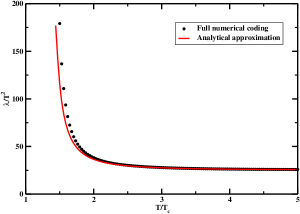
Figure 6: Thermal conductivity using various EOSs as a function of $T/T_{c}$.

The results of thermal conductivity displayed as a function of temperature in Fig.(6). Like other two previous cases, here too the analytical approximation works wonderfully well, showing convincing agreement with full numerical coding. We have plotted the dimensionless quantity $\lambda/T^{2}$ as a function of $T/T_{c}$ in the second plot, for all possible EOSs and both zero and nonzero quark chemical potentials. As before, the different EOSs are providing recognizably different effects at lower temperatures which are fusing with the ideal one at higher temperatures. The nonzero $\mu_{q}$ effects are only visible at quite low temperatures. Around $T/T_{c}\sim 2$, the LEOS results with $\mu_{q}=0.1$GeV is in good agreement with the NJL estimation of thermal conductivity by Marty Marty .

2.3.4 Electrical conductivity

In order to estimate $\sigma_{el}$, we start with the expression of diffusion flow given in Eq.(32). We clearly observe that at leading order with equilibrium distribution function $f_{k}^{0}$ in the definition of $N_{k}^{\mu}$, $N^{\mu}$ and $x_{k}$, the diffusion flow vanishes, while in the next to leading order the correction term $\delta f_{k}=f_{k}^{0}(1\pm f_{k}^{0})$, gives finite contribution to the diffusion flow as follows,

$$I_{a}^{\mu}=\sum_{k=1}^{N}(q_{ak}-x_{a})\int\frac{d^{3}\vec{p_{k}}}{(2\pi)^{3}p_{k}^{0}}p_{k}^{\mu}f_{k}^{0}(1\pm f_{k}^{0})\phi_{k}~{}.$$ (72)

Putting the value of $\phi_{k}$ from (52) with the help of Eq. (54) and (55) we get the linear law obeyed by the diffusion flow,

$$I_{a}^{\mu}=l_{aq}X_{q}^{\mu}+\sum_{b=1}^{N^{\prime}-1}l_{ab}X_{b}^{\mu}~{},a=1,....,(N^{\prime}-1)~{},$$ (73)

where the coefficients associated with thermal diffusion and particle concentration diffusion are given respectively as,

$$l_{aq}= \sum_{k=1}^{N}(q_{ak}-x_{a})\frac{1}{T}\int\frac{d^{3}\vec{p_{k}}}{(2\pi)^{3}}f_{k}^{0}(1\pm f_{k}^{0})\tau_{k}\frac{|\vec{p}_{k}|^{2}}{\omega_{k}^{2}}(\omega_{k}-h_{k})~{},$$ (74)

$$l_{ab}= \sum_{k=1}^{N}(q_{ak}-x_{a})(q_{bk}-x_{b})\frac{1}{T}\int\frac{d^{3}\vec{p_{k}}}{(2\pi)^{3}}f_{k}^{0}(1\pm f_{k}^{0})\tau_{k}\frac{|\vec{p}_{k}|^{2}}{\omega_{k}^{2}}.$$ (75)

Substituting the expression of diffusion flow from Eq.(73) into the microscopic definition of current density in Eq.(30), and pertaining the terms proportional to electric field only we finally obtain the expression for the electric current density as,

$$J^{\mu}=\sum_{k=1}^{N-1}(q_{k}-q_{N})[\sum_{l=1}^{N-1}l_{kl}\{q_{l}-q_{N}-\frac{h_{l}-h_{N}}{h}\sum_{n=1}^{N}x_{n}q_{n}\}-\frac{l_{kq}}{h}\sum_{n=1}^{N}x_{n}q_{n}]E^{\mu}~{}.$$ (76)

Finally comparing the Eq.(76) with the macroscopic definition of induced current density from Eq.(29) we get the expression for electrical conductivity as the following,

$$\sigma_{el}=\sum_{k=1}^{N-1}(q_{k}-q_{N})[\sum_{l=1}^{N-1}l_{kl}\{q_{l}-q_{N}-\frac{h_{l}-h_{N}}{h}\sum_{n=1}^{N}x_{n}q_{n}\}-\frac{l_{kq}}{h}\sum_{n=1}^{N}x_{n}q_{n}]~{}.$$ (77)

For a QGP system with quarks, antiquarks and gluons as the degrees of freedom, the expression of $\sigma_{el}$ turns out to be,

$$\sigma_{el}=q^{2}_{q}[ (l_{11}+l_{21})\{1-\frac{h_{q}-h_{g}}{h}(x_{q}+x_{\overline{q}})\}+(l_{12}+l_{22})\{1-\frac{h_{\overline{q}}-h_{g}}{h}(x_{q}+x_{\overline{q}})\}$$

$$- (l_{1q}+l_{2q})\frac{(x_{q}+x_{\overline{q}})}{h}]~{},$$ (78)

with,

$$l_{1q}= (1-x_{q})\frac{\tau_{q}}{T}\int\frac{d^{3}\vec{p_{q}}}{(2\pi)^{3}}f^{0}_{q}(1-f^{0}_{q})\frac{|\vec{p_{q}}|^{2}}{\omega_{q}^{2}}(\omega_{q}-h_{q})$$ (79)

$$+(-x_{q})\frac{\tau_{\overline{q}}}{T}\int\frac{d^{3}\vec{p_{\overline{q}}}}{(2\pi)^{3}}f^{0}_{\overline{q}}(1-f^{0}_{\overline{q}})\frac{|\vec{p_{\overline{q}}}|^{2}}{\omega_{\overline{q}}^{2}}(\omega_{\overline{q}}-h_{\overline{q}})$$

$$+(-x_{q})\frac{\tau_{g}}{T}\int\frac{d^{3}\vec{p_{g}}}{(2\pi)^{3}}f^{0}_{g}(1+f^{0}_{g})\frac{|\vec{p_{g}}|^{2}}{\omega_{g}^{2}}(\omega_{g}-h_{g})~{},$$

$$l_{2q}= (-x_{\overline{q}})\frac{\tau_{q}}{T}\int\frac{d^{3}\vec{p_{q}}}{(2\pi)^{3}}f^{0}_{q}(1-f^{0}_{q})\frac{|\vec{p_{q}}|^{2}}{\omega_{q}^{2}}(\omega_{q}-h_{q})$$ (80)

$$+(1-x_{\overline{q}})\frac{\tau_{\overline{q}}}{T}\int\frac{d^{3}\vec{p_{\overline{q}}}}{(2\pi)^{3}}f^{0}_{\overline{q}}(1-f^{0}_{\overline{q}})\frac{|\vec{p_{\overline{q}}}|^{2}}{\omega_{\overline{q}}^{2}}(\omega_{\overline{q}}-h_{\overline{q}})$$

$$+(-x_{\overline{q}})\frac{\tau_{g}}{T}\int\frac{d^{3}\vec{p_{g}}}{(2\pi)^{3}}f^{0}_{g}(1+f^{0}_{g})\frac{|\vec{p_{g}}|^{2}}{\omega_{g}^{2}}(\omega_{g}-h_{g})~{},$$

$$l_{11}=(1-x_{q})^{2}\frac{\tau_{q}}{T}\int\frac{d^{3}\vec{p_{q}}}{(2\pi)^{3}}f^{0}_{q}(1-f^{0}_{q})\frac{|\vec{p_{q}}|^{2}}{\omega_{q}^{2}}$$

$$+x_{q}^{2}\frac{\tau_{\overline{q}}}{T}\int\frac{d^{3}\vec{p_{\overline{q}}}}{(2\pi)^{3}}f^{0}_{\overline{q}}(1-f^{0}_{\overline{q}})\frac{|\vec{p_{\overline{q}}}|^{2}}{\omega_{\overline{q}}^{2}}$$

$$+x_{q}^{2}\frac{\tau_{g}}{T}\int\frac{d^{3}\vec{p_{g}}}{(2\pi)^{3}}f^{0}_{g}(1+f^{0}_{g})\frac{|\vec{p_{g}}|^{2}}{\omega_{g}^{2}}~{},$$ (81)

$$l_{22}= x_{\overline{q}}^{2}\frac{\tau_{q}}{T}\int\frac{d^{3}\vec{p_{q}}}{(2\pi)^{3}}f^{0}_{q}(1-f^{0}_{q})\frac{|\vec{p_{q}}|^{2}}{\omega_{q}^{2}}$$ (82)

$$+(1-x_{\overline{q}})^{2}\frac{\tau_{\overline{q}}}{T}\int\frac{d^{3}\vec{p_{\overline{q}}}}{(2\pi)^{3}}f^{0}_{\overline{q}}(1-f^{0}_{\overline{q}})\frac{|\vec{p_{\overline{q}}}|^{2}}{\omega_{\overline{q}}^{2}}$$

$$+x_{\overline{q}}^{2}\frac{\tau_{g}}{T}\int\frac{d^{3}\vec{p_{g}}}{(2\pi)^{3}}f^{0}_{g}(1+f^{0}_{g})\frac{|\vec{p_{g}}|^{2}}{\omega_{g}^{2}}~{},$$

and

$$l_{12}=l_{21}= x_{\overline{q}}(x_{q}-1)\frac{\tau_{q}}{T}\int\frac{d^{3}\vec{p_{q}}}{(2\pi)^{3}}f^{0}_{q}(1-f^{0}_{q})\frac{|\vec{p_{q}}|^{2}}{\omega_{q}^{2}}$$ (83)

$$+x_{q}(x_{\overline{q}}-1)\frac{\tau_{\overline{q}}}{T}\int\frac{d^{3}\vec{p_{\overline{q}}}}{(2\pi)^{3}}f^{0}_{\overline{q}}(1-f^{0}_{\overline{q}})\frac{|\vec{p_{\overline{q}}}|^{2}}{\omega_{\overline{q}}^{2}}$$

$$+x_{q}x_{\overline{q}}\frac{\tau_{g}}{T}\int\frac{d^{3}\vec{p_{g}}}{(2\pi)^{3}}f^{0}_{g}(1+f^{0}_{g})\frac{|\vec{p_{g}}|^{2}}{\omega_{g}^{2}}~{}.$$

The $q_{q}^{2}=\sum_{k}\nu_{k}q_{qk}^{2}$ is simply the square of the fractional quark charges taking sum over quark degeneracy. For up, down and strange quarks the fractions quark charges are taken to be $2/3$, $-1/3$ and $-1/3$ respectively.

Apart of the full numerical coding, we have done the analytical approximation as well in estimating the value of $\sigma_{el}$. For this purpose the two relevant integrals present in Eq.(79)-(83), indicated by $I_{1}$ and $I_{2}$ as following,

$$\{I_{1}\}_{k}= \int\frac{d^{3}\vec{p_{k}}}{(2\pi)^{3}}f^{0}_{k}(1\pm f^{0}_{k})\frac{|\vec{p_{k}}|^{2}}{\omega_{k}^{2}}(\omega_{k}-h_{k})~{},$$ (84)

$$\{I_{2}\}_{k}= \int\frac{d^{3}\vec{p_{k}}}{(2\pi)^{3}}f^{0}_{k}(1\pm f^{0}_{k})\frac{|\vec{p_{k}}|^{2}}{\omega_{k}^{2}}~{},$$ (85)

are needed to be computed analytically as indicated earlier. The estimated values of the integrals for different partonic degrees of freedom in terms of the fugacity parameters and its derivatives are given below

$$\{I_{1}\}_{g}= -\frac{T^{4}}{\pi^{2}}[\textrm{PolyLog}[3,z_{g}]-\frac{2}{3}\{(\frac{T}{T_{c}})\partial_{(\frac{T}{T_{c}})}(lnz_{g})\}\textrm{PolyLog}[2,z_{g}]]~{},$$ (86)

$$\{I_{1}\}_{q}= \frac{T^{4}}{\pi^{2}}[\textrm{PolyLog}[3,-z_{q}]+\tilde{\mu_{q}}\textrm{PolyLog}[2,-z_{q}]-\frac{{\tilde{\mu_{q}}}^{2}}{2}ln(1+z_{q})]$$ (87)

$$-\frac{2T^{4}}{3\pi^{2}}\{(\frac{T}{T_{c}})\partial_{(\frac{T}{T_{c}})}(lnz_{q})\}[\textrm{PolyLog}[2,-z_{q}]-\tilde{\mu_{q}}ln(1+z_{q})-\frac{{\tilde{\mu_{q}}}^{2}}{2}\frac{z_{q}}{1+z_{q}}]~{},$$

$$\{I_{1}\}_{\overline{q}}= \frac{T^{4}}{\pi^{2}}[\textrm{PolyLog}[3,-z_{q}]-\tilde{\mu_{q}}\textrm{PolyLog}[2,-z_{q}]-\frac{{\tilde{\mu_{q}}}^{2}}{2}ln(1+z_{q})]$$ (88)

$$-\frac{2T^{4}}{3\pi^{2}}\{(\frac{T}{T_{c}})\partial_{(\frac{T}{T_{c}})}(lnz_{q})\}[\textrm{PolyLog}[2,-z_{q}]+\tilde{\mu_{q}}ln(1+z_{q})-\frac{{\tilde{\mu_{q}}}^{2}}{2}\frac{z_{q}}{1+z_{q}}]~{},$$

$$\{I_{2}\}_{g}= \frac{T^{3}}{\pi^{2}}\textrm{PolyLog}[2,z_{g}]+\frac{T^{3}}{\pi^{2}}\{(\frac{T}{T_{c}})\partial_{(\frac{T}{T_{c}})}(lnz_{g})\}ln(1-z_{g})~{},$$ (89)

$$\{I_{2}\}_{q}= \frac{-T^{3}}{\pi^{2}}[\textrm{PolyLog}[2,-z_{q}]-\tilde{\mu_{q}}ln(1+z_{q})-\frac{{\tilde{\mu_{q}}}^{2}}{2}\frac{z_{q}}{1+z_{q}}]$$ (90)

$$-\frac{T^{3}}{\pi^{2}}\{(\frac{T}{T_{c}})\partial_{(\frac{T}{T_{c}})}(lnz_{q})\}[ln(1+z_{q})+\tilde{\mu_{q}}\frac{z_{q}}{1+z_{q}}+\frac{{\tilde{\mu_{q}}}^{2}}{2}\frac{z_{q}}{(1+z_{q})^{2}}]~{},$$

$$\{I_{2}\}_{\overline{q}}= \frac{-T^{3}}{\pi^{2}}[\textrm{PolyLog}[2,-z_{q}]+\tilde{\mu_{q}}ln(1+z_{q})-\frac{{\tilde{\mu_{q}}}^{2}}{2}\frac{z_{q}}{1+z_{q}}]$$ (91)

$$-\frac{T^{3}}{\pi^{2}}\{(\frac{T}{T_{c}})\partial_{(\frac{T}{T_{c}})}(lnz_{q})\}[ln(1+z_{q})-\tilde{\mu_{q}}\frac{z_{q}}{1+z_{q}}+\frac{{\tilde{\mu_{q}}}^{2}}{2}\frac{z_{q}}{(1+z_{q})^{2}}]~{}.$$

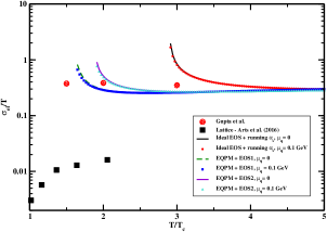
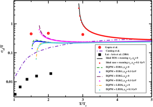
Figure 7: Electrical conductivity using various EOSs as a function of $T/T_{c}$.

We end this section by giving the results of electrical conductivity in Fig.(7). The dimensionless ratio $\sigma_{el}/T$ has been plotted against $T/T_{c}$ for $N_{f}=2$ and $N_{f}=3$ employing different EOSs in the EQPM. The results with $\mu_{q}=0.1$ GeV differ from the same with $\mu_{q}=0$ as given in Mitra-Chandra , below $T/T_{c}\sim 2$, in a small but quantitative amount. The 3-flavor case appears to be slightly greater than the 2-flavor ones, since the quark charge $q_{q}^{2}$ in Eq. (78) includes the fractional quark charge of strange quark also. At lower temperature the lattice data from Aarts1 is observed to under predict the current results, however the quenched lattice estimations of electrical conductivity from Gupta et al. Gupta1 agrees with the current estimation of $\sigma_{el}$ quite sensibly. For 3-flavor case beyond $T/T_{c}\sim 3$, the estimations of $\sigma_{el}$ is matching with the trend given in Cassing et al. Cassing1 and agrees with their statement that above $T\sim 5T_{c}$ the dimensionless ratio $\sigma_{el}/T$ becomes approximately constant ($\approx 0.3$). In the estimations of $\sigma_{el}$ throughout, the electronic charges are explicitly given by the relation $\frac{e^{2}}{4\pi}=\frac{1}{137}$.

3 Ratios of transport coefficients and related physical laws

This section deals with the highlights on relative important of various transport parameters computed in the previous sections. In a nutshell, the relative importance of the charge diffusion, the momentum diffusion and the heat diffusion in a hot QCD medium are being explored by studying the ratios of various transport coefficients, explicated below.

3.1 Thermal diffusion vs charge diffusion: The ratio $\lambda/{\sigma_{el}T}$

The relation between electrical conductivity, $\sigma_{el}$ and thermal conductivity, $\lambda$ for any substance can be understood in terms of the Wiedemann-Franz law. The basic mathematical statement of the law is,

$$\frac{\lambda}{\sigma_{el}T}={\mathbf{L}}\ \ [{\mathbf{L}}:\text{Lorenz number}]$$ (92)

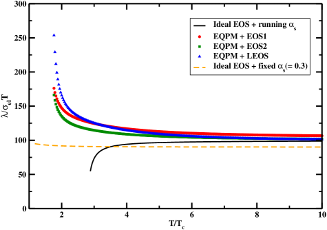
Figure 8: Lorentz number using various EOSs as a function of $T/T_{c}$.

For instance, in the case of metals, ${\mathbf{L}}$ is a constant and quantifies the fact that metals are good electrical as well thermal conductors. In general cases, where the system under consideration, does not possess a high symmetry (for e.g. an anisotropic crystal), both $\lambda$ and $\sigma_{el}$ are tensorial quantities (rank-2 tensors), in effect, ${\mathbf{L}}$ will be a forth rank tensor. In the case of hot QCD medium, it is possible to compute both of these transport coefficients independently either within field theory approach or transport theory with Chapman-Enskog technique (or any other equivalent method). As shown earlier, here, the latter approach has been utilized. The main aim here is to investigate, whether the hot QCD medium/QGP also follow the above mentioned law. If there are deviations, what interesting aspects could emerge while understanding the quantum aspects of its liquidity. The temperature dependence of the Lorentz number for the QGP is depicted in Fig. 8. For the temperature range $2-10\ T_{c}$, ${\mathbf{L}}$ varies between $250-100$ for various realistic QGP EOSs. For $T\geq 4T_{c}$ the number saturates closer to a value $100$ which is also the Stefan-Boltzmann (SB) limit (QGP as a ultra-relativistic gas of gluons and quarks). Clearly, the violation is quite apparent for the temperatures which are smaller than $4T_{c}$ (in fact the violation becomes quite prominent while moving towards $2T_{c}$). The law in the case of the QGP mainly depends on the effective coupling, the EOS chosen and the contributions that are included while computing the thermal relaxation times. To make any sensible argument about the violation and its connection with the other Wiedemann-Franz law violating quantum fluids such as graphene Crossno , a more through and deeper analysis is needed (inclusion of higher order QCD processes and appropriate collision and source terms in the transport equation and also effects from momentum anisotropy). Nevertheless, the observation from our study perhaps indicates towards much more complex nature of the QGP as a strongly interacting quantum fluid for the temperatures that not very large as compared to the QCD transition temperature, $T_{c}$. Noticeably, such deviations have also been observed in holographic anisotropic models that are dual to spatially anisotropic, ${\cal N}=4$ Super Yang-Mills theory at finite chemical potential XianGe which further violates the KSS bound of $\eta/S$ in the longitudinal direction. Further, within the holographic set up while considering the charged black holes, Jain Sachin-cond1 ; Sachin-cond2 has been able to show that thermal and electrical conductivities show universal properties and so their universal ratio in higher dimension. The number obtained in Fig. 8 are slightly higher as compared to those from holographic models Son1 , by holographic estimates.

3.2 Momentum diffusion vs charge diffusion

The relative significance of the momentum diffusion and the charge diffusion in a medium, could be understood in terms of a dimensionless ratio,

$${\mathcal{R}}_{\eta/\sigma_{el}}=\frac{\eta/S}{\sigma_{el}/T}.$$ (93)

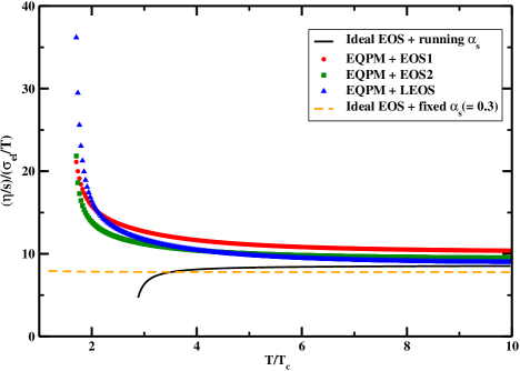
Figure 9: Shear viscosity to entropy ratio vs Electrical conductivity as a function of $T/T_{c}$.

In a hot QCD medium, unlike gluons, a quark (antiquark) carries EM charge. Therefore, it is reasonable to expect that their contribution to the $\sigma_{el}$ would be predominant as gluons enter only through the interactions ($qg$ and $gg$ scattering contributions). Since the gluonic scattering rates are larger as compared to that for the quarks and antiquarks, hence the quark contribution to the shear viscosity is also expected to be dominant. The ratio, ${\mathcal{R}}_{\eta/\sigma_{el}}$ could be an indicator of relative significance of the gluonic and matter sector as far as the relative importance of the momentum and the charge transports in the QGP medium are concerned. This point has been realized in some degree of detail in Greco where a scaling in terms of gluon and quark relaxation times was seen. In contrast, in the present analysis, such a scaling highlighting the relative importance of gluonic and quark contributions is not expected due to more systematic treatment of the scattering cross-sections and computation of relaxation times and inclusion of all the relevant effects from gluonic sector. The ratio decreases with increasing temperature and subsequently saturating towards the SB limit (the black line in Fig. 9). The ratio is always greater than unity for the whole range of temperature. It can be inferred that the momentum transfer has dominant impact over the charge diffusion.

3.3 Momentum diffusion vs thermal diffusion: The Prandtl number for the QGP

The relative magnitude of the momentum and the thermal diffusions is quantified in terms of Prandtl number, $Pr$ (the ratio of momentum diffusibility by thermal diffusibility):

$$Pr=\frac{\eta\ c_{p}}{\rho\ \lambda},$$ (94)

where $c_{p}$ is the specific heat at constant pressure. This number signifies the relative importance of the shear viscosity and the thermal conductivity in the sound attenuation in a liquid medium. Before, describing it for a hot QCD/QGP medium, let us have an idea about its magnitude for other strongly coupled systems. For liquid Helium the Prandtl number is around $2.5$ Schafer2 , for weakly interacting unitary Fermi gas at high temperature, it is $2/3$ Schafer2 ; schafer . On the other hand for conformal non-relativistic theories, the number is of the order of $1$ Son2 .

To define Prandtl number for the QGP, apart from $\eta$ and $\sigma$, and $c_{p}$, one requires to know the mass density, $\rho$. The only mass scale in high temperature QCD is the thermal mass of a dressed parton (gluon or quark) that is obtained in terms of the QCD effective coupling constant at high temperature and the temperature scale of the system. In our case, the mass density for the QGP can be defined as,

$$\rho=m_{g}\ n_{g}+m_{q}\ (n_{q}+n_{\bar{q}}),$$ (95)

where, $m_{g}$ and $m_{q}$ are the thermal(medium) masses of the gluons and quarks respectively and $n_{g}$, $n_{q,\bar{q}}$ are their respective number densities obtained from the momentum distributions, following the basic thermodynamic definitions.

Figure 10: Pr.No. using various EOSs as a function of $T/T_{c}$.

The gluon medium mass $m_{g}$ and quark medium mass, $m_{q}$ for the QCD are obtained in terms of gluon and quark/antiquark distributions functions as greiner_dm

$$m_{g}^{2}(=m_{D}^{2})\equiv 4\pi\alpha_{s}(T,\mu_{q})\bigg{\{}-2N_{c}\int\frac{d^{3}\vec{p}}{(2\pi)^{3}}\partial_{p}f_{g}(\vec{p})-N_{f}\int\frac{d^{3}p}{(2\pi)^{3}}\partial_{p}(f_{q}(\vec{p})+f_{\bar{q}}(\vec{p}))\bigg{\}}$$

$$m_{q}^{2} = \bigg{(}\frac{N_{c}^{2}-1}{2N_{c}}\bigg{)}4\pi\alpha_{s}(T,\mu_{q})\int\frac{d^{3}\vec{p}}{(2\pi)^{3}|\vec{p}|}\bigg{\{}f_{g}(\vec{p})+\bigg{(}\frac{f_{q}(\vec{p})+f_{\bar{q}}(\vec{p})}{2}\bigg{)}\bigg{\}}.$$ (96)

The number density and specific heat computations are presented in the appendix. The number is plotted as a function of $T/T_{c}$ in Fig. 10 for various EOSs within their EQPM descriptions. The number is in the range $20-35$ for the all cases considered here. All the other liquids/systems mentioned previously possess much smaller numbers as compared to the QGP, therefore sound attenuation is mostly governed by the momentum diffusion here. In this context, we may perhaps, ignore the effects that are coming out from thermal diffusion unlike holographic models where both these effects are at an equal footing.

4 Results and discussions

The temperature dependences of the viscosities, conductivities and their mutual ratios obtained so far leads to a situation where our results are needed to be analyzed in the light of the estimations of these quantities employing various discrete techniques, available in existing literature. In the following, the results regarding different transport parameters and the corresponding physical laws are discussed subsequently.

• As earlier experimental predictions of viscosity values, Luzum introduces $\eta/s=0.08$ and $0.16$ in their 2+1 dimensional viscous hydrodynamic code using Glauber and CGC initial conditions respectively, for explaining the elliptic flow data of charged hadron from STAR and PHOBOS. Ref. Heinz , in their work has concluded a robust upper limit $(\eta/s)_{QGP}<\frac{5}{4\pi}$ by analyzing the phenomenological aspects to be compatible with the experimental $v_{2}$ data. Ref. Song has obtained a range $\frac{1}{4\pi}<(\eta/s)_{QGP}<\frac{2.5}{4\pi}$ in their hybrid code ((VISH2+1)+URQMD), in order to describe the charged hadron multiplicity density obtained from 200 GeV, Au+Au RHIC data. In Denicol , the reported value is, $\eta/s\simeq 0.5$, which when implemented in hydrodynamic simulation approves the multiplicity and collective flow data of charged hadrons from PHOBOS. Rischke shows a temperature dependence of $\eta/s$ in explaining the transverse momentum spectra and elliptic flow of hadrons in RHIC. ALICE predictions ALICE1 ; ALICE2 ; ALICE2 ; ALICE4 ; ALICE5 ; ALICE-JHEP mostly reports $\eta/s\simeq 0.2$. The analysis of BAMPS data in Greiner2 gives $\eta/s=0.15$ at $\alpha_{s}=0.3$. The lattice prediction by Nakamura for pure glue leads to $\eta/s\simeq 0.08-0.75$ around $T_{c}$. In comparison to all these experimental extractions and lattice simulations, the values of $\eta/s$ obtained from all the pQCD based studies AMY1 ; AMY2 ; Chen1 ; Chen2 ; Greiner1 ; Greco ; Hirano2 are at least a factor of 5-10 times larger. Mostly leading log results with bare particles results $\eta/s\sim 1$, where in AMY2 the medium properties folded within the hard thermal loops of exchanged propagator leads to $\eta/s\sim 2.7$ at $\alpha_{s}\simeq 0.1$. So hence we conclude that the EQPM model, which is basically dressing up the bare particles by defining their collective properties in a thermal medium, and those properties are being reflected through the logarithmic term in the viscosity, is responsible for the large values ($\sim 2$) of $\eta/s$. Nevertheless, these are comparable with other estimates based on effective field theory estimations at high temperature.

• In all the estimations of bulk viscous coefficient the value of $\zeta/s$ has been reported extremely smaller except near $T_{c}$. In Ryu , the 3D hybrid simulation agrees with data from ALICE and CMS for $\zeta/s\approx 0.3$ around $T_{c}$. The lattice Monte Carlo calculation for $SU(3)$ gluodynamics in Meyer reports $\zeta/s<0.15$ near $T_{c}$ ($T/T_{c}=1.65$) which becomes negligibly small $\zeta/s<0.015$ away from $T_{c}$. The leading order pQCD estimation from ADY also gives small value of bulk viscosity, $\zeta=0.2\alpha_{s}^{2}T^{3}$ for reasonable perturbative value of $0.2\lesssim\alpha_{s}\lesssim 0.3$. Our estimation of $\zeta$ in the current work mostly consistent with these results giving considerable magnitude only below $T/T_{c}\sim 2$. Regarding the scaling law obeyed by the ratio $\zeta/\eta$, most of the relativistic hydrodynamic calculations Weinberg , pQCD estimations ADY and the flow harmonics studies from experimental data Rose follow the scaling-2 ($\sim\{\frac{1}{3}-c_{s}^{2}\}^{2}$), whereas ADS/CFT based measurements mostly report the scaling-1 ($\sim\{\frac{1}{3}-c_{s}^{2}\}$) Benincasa ; Gubser . In our study we observed that $\eta/\zeta$ ratio is more consistent with the scaling-2 at higher temperatures. However, at lower temperature ranges non of the scaling works indicating the peculiar nature of the QGP as a strongly coupled quantum fluid.

• In comparison to the viscosities, the investigations on thermal conductivity are really quite limited in the existing literature. In Greif , the $\lambda$ of a massless Boltzmann gas using partonic cascade model has been listed as a temperature independent quantity for a number of isotropic cross sections. In Marty , the dimensionless quantity, $\lambda/T^{2}$ has been plotted against $T/T_{c}$ from for both NJL model and dynamical quasiparticle particle model (DQPM), which displays two completely different trends. However, at lower temperature ranges ($T/T_{c}\sim 1.5-2.5$), our estimations appear to be quite consistent at the quantitative level with the NJL one.

• As a prime signature of electromagnetic responses in the heavy ion collision, the estimation of $\sigma_{el}$ has achieved a considerable amount of attention now a days in the QGP related fields. The lattice data from Amato ; Aarts1 ; Aarts2 ; Brandt1 ; Brandt2 ; Ding provide an estimation for $\sigma_{el}/T$ that is below $0.05$, upto temperature $350$ MeV, which quite under predict our results but the quenched lattice estimation from Gupta1 offers quite sensible agreement. The DQPM results from Cassing1 also exhibits compatible trend with our result. The maximum entropy method (MEM) by Qin gives $\sigma_{el}/T\sim 0.4$ at $T/T_{c}=3$ which is also close to our result. In Kharzeev2 , the sensitivity of early stage strong magnetic field in non central heavy ion collisions have been tested on the azimuthal distributions and correlations of the produced charged hadrons. In their analysis they have chosen the electric conductivity $\sigma_{el}=0.023fm^{-1}$ in order to obtain the directed flow ($v_{1}$) of charged pions at LHC energies which is not away from our estimations around a temperature region $T/T_{c}\sim 2.5$.

• Interplay of the thermal diffusion and the electrical diffusion could be understood in terms of the Wiedemann-Franz law–the dimensionless number (Lorentz number). For a large class of metals this is constant and depicts the common origin of both the transport processes. In other words, the metals are good thermal and electrical conductors at the same time. The number for the hot QCD system in the current works converges to a number slightly higher than $100$ at higher temperatures. For the temperatures that are lower than $3T_{c}$, there is significant rise as we decrease the temperature. This indicates, towards the violation of the above mentioned law. In some known systems, such as Graphene this violation leads to a strongly interacting quantum fluid also termed as Dirac fluid Crossno . In this present case, the violation is mainly due to the $1/\alpha_{s}$ term and the strongly interacting EOS. To make any such concrete connection with the other interesting quantum fluids is quite early as it will require more refined computation of the Lorenz number while including higher order hot QCD effects to the current analysis. This will be one direction where the future investigation will focus on. In order to explore the relative importance of the momentum diffusion and the charge diffusion in the hot QCD medium, ratio of $\eta/s$ to $\sigma_{el}/T$ is studied as a function of temperature. The ratio for the QGP is turned out to be much greater than unity for the whole range of the temperature considered here indicating the more prominent role of the momentum diffusion in agreement to the prediction of  Greco . Finally the relative significance of the thermal and the momentum diffusions has been quantified in terms of Prandtl number. For the hot QCD system here, this number came out to be much greater than unity signifying the dominance of the momentum diffusion over thermal one. In other words, sound attenuation in the hot QCD/QGP system will mainly be governed by the shear viscous effects which is in contrast to the observations for dilute fermi-gases Schafer2 or the holographic systems Son2 . For e.g. in liquid Helium, the number is $2.5$ Schafer2 which is but an order of magnitude smaller.

5 Conclusions and outlook

The current article concerns about the temperature behavior of various transport coefficients that measures the dissipative and electromagnetic responses in a strongly interacting QCD system at finite temperature with non zero quark chemical potential. The most important feature of this work is to highlight the concerning physical laws expressing the relative importance of different transport phenomena, by obtaining the temperature dependences of their mutual ratios. The detail Chapman-Enskog technique for a multi-component fluid, adopted from the kinetic theory of many particle systems has been discussed which gives the mathematical expressions of shear and bulk viscosities, thermal conductivity and electrical conductivity in terms of the medium interactions. The interaction cross sections are provided through the thermal relaxation times of constituent quarks, antiquarks and gluon by leading order QCD estimations. The effects of a strongly couped thermal medium has been introduced in the evaluation of these transport parameters through the EQPM model, which describes the collective properties of quarks and gluons by considering them as quasi particles rather than bare ones. The finite temperature effects have been folded through this EQPM scheme by introducing the pQCD and Lattice QCD based equation of state effects in particle momentum distribution and effective couplings. Finally they are applied to the current formalism of estimating transport coefficients and studying the related physical laws. So we conclude by saying that we have investigated the transport properties and electromagnetic responses along with the associated physical laws in a strongly interacting hot QCD medium quite throughly and reasonably, presenting a sensible realistic scenario created out of the relativistic heavy ion collisions. The results obtained in our approach are seen to be consistent with other parallel or distinct approaches.

The current work opens a horizon of possible extensions and applications in the related areas in near future. A few interesting ones are listed below which could be a matter of immediate future investigations.

• All the above mentioned transport coefficients have wide spread applications in signal extractions by affecting the quantitative estimates of the signals for QGP from heavy ion collisions, particularly, where hydrodynamic simulations are involved. In Dusling1 ; Dusling2 ; Dusling3 ; Bhatt-Mishra ; Dion-Gale ; Sarkar-Alam ; Mitra-photon ; Denicol-2017 , the effect of viscosities have been tested on transverse momentum spectra and collective flows of charged hadron and electromagnetic probes rigorously, revealing the necessity of incorporating them in the out of equilibrium particle distribution functions and dissipative hydrodynamics. They are observed to modify the collective behavior of plasma as well, such as in Strickland viscous corrections are shown to affect Debye screening and Landau damping mass scales and in Torrieri leads to clusterization and early freeze out of the QGP. In Bhatt-cavitation ; Rajagopal it is discussed that the viscous effects lead to fluid cavitation predicting the breakdown of hydrodynamic calculations. In Skokov-th the effect of $\lambda$ is studied in the dynamics of first-order phase transitions. In Yin ; Ding ; Huot the soft photon and dilepton emission rates are shown to depend up on $\sigma_{el}$ so that their transverse momentum spectra and elliptic flow are also sensitive on the temperature dependence of $\sigma_{el}$. In the light of the above analysis, implementation of the obtained temperature dependence of transport parameters, in the particle emission rates and in the hydrodynamic evolution codes as well as in the collective mode measurements, is aimed to be a matter of immediate future investigation.

• Realizing the high event statistics and high precision knowledge offered by relativistic heavy ion collisions where the application of the usual Boltzmann-Gibbs statistics is questionable, the inclusion of a nonextensive statistical model Wilk1 ; Tsallis ; Biro is necessary via Tsallis distribution. So all the definitions of thermodynamic and transport quantities used in this article are to be revisited for a dynamical, non-equilibrium system with strong intrinsic fluctuations and long-range correlations.

• The collision term is needed to be re looked by keeping the instantaneous charge and energy-momentum conservation consistent BGK and including appropriate Vlasov term and source contributions in order to study the production and evolution of QGP. There may be possibilities to exclude the relaxation time technique as a whole and treat the collision term by explicit polynomial expansion using variational method Degroot .

• The viscosities controlling the magnitude of hydrodynamic fluctuations in the fluid can be extracted directly from the correlation observables in heavy ion collisions Kapusta-fluctuation . This can offer a means to predict the viscosity, independent from the traditional collective flow analysis and can shed some light regarding the dissimilarities in the viscosity values extracted by them from the pQCD measurements.

• Finally, the estimations of all the above mentioned transport coefficients by including higher order thermal QCD effects with an appropriate collision, Vlasov and source terms in the transport equation also including the anisotropic aspects of the QGP in heavy-ion collisions could be another interesting direction where the future explorations could focus on.

Appendix A Evolution equation of thermodynamic quantities and conservation laws

The conservation laws and the consequent time evolution equations for the thermodynamic macroscopic quantities which define the state of the system have been enlisted below. In order to determine the transport coefficients in Chapman-Enskog technique, these equations of motions have been used as the thermodynamic identities in Section 2.3.

In order to do this we start with the relativistic transport equation in presence of the external electric field,

$$p_{k}^{\mu}\partial_{\mu}f_{k}^{0}+\frac{1}{T}f_{k}^{0}(1\pm f_{k}^{0})q_{k}E_{\mu}p_{k}^{\mu}=\sum_{l=1}^{N}C_{kl}[f_{k},f_{l}],~{}~{}~{}~{}~{}~{}~{}~{}~{}~{}~{}~{}~{}~{}~{}~{}[k=1,2,..........N]~{}.$$ (97)

Integrating both sides of Eq.(97) over $\int\frac{d^{3}p}{(2\pi)^{3}p_{k}^{0}}$ and summing over $\sum_{k=1}^{N}$, the right hand side of Eq.(97) vanishes, since the first moment of collision term is zero by the virtue of summational invariants. Finally what we left with is the conservation of particle number as the following,

$$\partial_{\mu}N^{\mu}=0~{}.$$ (98)

In a system where the number of particles of each components are conserved separately, like the current system where only elastic collisions are being considered, we obtain,

$$\partial_{\mu}N_{k}^{\mu}=0~{}~{}~{}~{}~{}~{}~{}~{}[k=1,....,N].$$ (99)

From Eq.(99) the continuity equation, i.e, the evolution equation of the particle number density for each species can be obtained in the following manner,

$$Dn_{k}=-n_{k}\partial\cdot u~{}.$$ (100)

In an analogous way, multiplying both sides of Eq.(97) with $p_{k}^{\nu}$, integrating over $\int\frac{d^{3}p}{(2\pi)^{3}p_{k}^{0}}$ and summing over $\sum_{k=1}^{N}$, the right hand side of Eq.(97) again vanishes, since the second moment of collision term is zero also. Finally contracting the resulting equation with $u_{\nu}$ from left we get,

$$u_{\nu}\partial_{\mu}T^{\mu\nu}=0~{},$$ (101)

where $T^{\mu\nu}$ is the energy-momentum stress tensor. From Eq.(101) the equation of energy evolution of the system can be easily traced out as,

$$\sum_{k=1}^{N}x_{k}D\omega_{k}=-\frac{\sum_{k=1}^{N}P_{k}}{\sum_{k=1}^{N}n_{k}}\partial\cdot u~{}.$$ (102)

In the second case a contraction with $\Delta^{\sigma}_{\nu}$ from left gives,

$$\Delta^{\sigma}_{\nu}\partial_{\mu}T^{\mu\nu}+E^{\sigma}\sum_{k=1}^{N}q_{k}n_{k}=0~{},$$ (103)

from which in a multicomponent system in the presence of an electric field the equation of motion becomes,

$$Du^{\mu}=\frac{\nabla^{\mu}P}{\sum_{k=1}^{N}n_{k}h_{k}}+\frac{\sum_{k=1}^{N}q_{k}n_{k}}{\sum_{k=1}^{N}h_{k}n_{k}}E^{\mu}~{}.$$ (104)

Clearly even the pressure gradient is zero, the Lorentz force acting on the electrically charged particle produces non-zero acceleration.

Appendix B Thermodynamical quantities at finite chemical potential, $\mu_{q}$

Here, the expressions for the thermodynamic quantities are presented following their fundamental definitions, within EQPM at finite $\mu_{q}$. These quantities have been used throughout the article during the formalism development. The quantities under consideration are , viz., particle number density, pressure, energy density, enthalpy density, entropy density, specific heat at constant pressure and the velocity of sound. To compute these quantities, we need their definitions in terms of EQPM degrees of freedom. Following the corresponding definitions of the particle number density, pressure and energy density, we can straightforwardly derive all the quantities mentioned here.

The particle number density, $n$ is obtained as,

$$n= \sum_{k=g,q,\overline{q}}\nu_{k}\int\frac{d^{3}\vec{p_{k}}}{(2\pi)^{3}}f^{0}_{k}$$ (105)

$$= \frac{T^{3}}{\pi^{2}}[\nu_{g}\textrm{PolyLog}[3,z_{g}]-\nu_{q}\{2\textrm{PolyLog}[3,-z_{q}]-{\tilde{\mu_{q}}}^{2}ln(1+z_{q})\}]~{}.$$ (106)

On the other hand, Pressure, $P$ and the energy density, $\epsilon$, following their respective fundamental definitions can be obtained as,

$$P= \sum_{k=g,q,\overline{q}}\frac{1}{3}\nu_{k}\int\frac{d^{3}\vec{p_{k}}}{(2\pi)^{3}p_{k}^{0}}|\vec{p_{k}}|^{2}f^{0}_{k}$$ (107)

$$= \frac{T^{4}}{\pi^{2}}[\nu_{g}\textrm{PolyLog}[4,z_{g}]-\nu_{q}\{2\textrm{PolyLog}[4,-z_{q}]+{\tilde{\mu_{q}}}^{2}\textrm{PolyLog}[2,-z_{q}]\}]~{}.$$ (108)

$$\epsilon= \sum_{k=g,q,\overline{q}}\nu_{k}\bigg{[}\int\frac{d^{3}\vec{p_{k}}}{(2\pi)^{3}p_{k}^{0}}{(p_{k}^{0})}^{2}f^{0}_{k}+T\big{\{}\frac{T}{T_{c}}\big{\}}\{\partial_{(\frac{T}{T_{c}})}(lnz_{k})\}\int\frac{d^{3}\vec{p_{k}}}{(2\pi)^{3}}f^{0}_{k}\bigg{]}$$ (109)

$$= \frac{3T^{4}}{\pi^{2}}[\nu_{g}\textrm{PolyLog}[4,z_{g}]-\nu_{q}\{2\textrm{PolyLog}[4,-z_{q}]+{\tilde{\mu_{q}}}^{2}\textrm{PolyLog}[2,-z_{q}]\}]$$ (110)

$$+T\{\frac{T}{T_{c}}\}\{\partial_{(\frac{T}{T_{c}})}(lnz_{g})\}[\frac{T^{3}}{\pi^{2}}\nu_{g}\textrm{PolyLog}[3,z_{g}]]$$

$$-T\{\frac{T}{T_{c}}\}\{\partial_{(\frac{T}{T_{c}})}(lnz_{q})\}[\frac{T^{3}}{\pi^{2}}\nu_{q}\{2\textrm{PolyLog}[3,-z_{q}]-{\tilde{\mu_{q}}}^{2}ln(1+z_{q})\}]~{}.$$

The enthalpy density, $H$, entropy density, $s$ and specific heat at constant pressure, $c_{p}$, could be obtained in terms of $P$ and $\epsilon$ as,

$$H= \epsilon+P$$ (112)

$$\frac{4T^{4}}{\pi^{2}}[\nu_{g}\textrm{PolyLog}[4,z_{g}]-\nu_{q}\{2\textrm{PolyLog}[4,-z_{q}]+{\tilde{\mu_{q}}}^{2}\textrm{PolyLog}[2,-z_{q}]\}]$$

$$+T\{\frac{T}{T_{c}}\}\{\partial_{(\frac{T}{T_{c}})}(lnz_{g})\}[\frac{T^{3}}{\pi^{2}}\nu_{g}\textrm{PolyLog}[3,z_{g}]]$$

$$-T\{\frac{T}{T_{c}}\}\{\partial_{(\frac{T}{T_{c}})}(lnz_{q})\}[\frac{T^{3}}{\pi^{2}}\nu_{q}\{2\textrm{PolyLog}[3,-z_{q}]-{\tilde{\mu_{q}}}^{2}ln(1+z_{q})\}]~{}.$$

$$s= \frac{\epsilon+P}{T}-\frac{n\mu}{T}$$ (114)

$$\frac{4T^{3}}{\pi^{2}}\nu_{g}\textrm{PolyLog}[4,z_{g}]-\frac{8T^{3}}{\pi^{2}}\nu_{q}\textrm{PolyLog}[4,-z_{q}]-\frac{2T^{3}}{\pi^{2}}{\tilde{\mu_{q}}}^{2}\nu_{q}\textrm{PolyLog}[2,-z_{q}]$$

$$+\{\frac{T}{T_{c}}\}\{\partial_{(\frac{T}{T_{c}})}(lnz_{g})\}[\frac{T^{3}}{\pi^{2}}\nu_{g}\textrm{PolyLog}[3,z_{g}]]$$

$$-\{\frac{T}{T_{c}}\}\{\partial_{(\frac{T}{T_{c}})}(lnz_{q})\}[\frac{T^{3}}{\pi^{2}}\nu_{q}\{2\textrm{PolyLog}[3,-z_{q}]-{\tilde{\mu_{q}}}^{2}ln(1+z_{q})\}]~{}.$$

$$c_{p}= \frac{\partial H}{\partial T}+\frac{\partial H}{\partial\mu_{q}}\tilde{\mu_{q}}$$ (115)

$$= \frac{16T^{3}}{\pi^{2}}\nu_{g}\textrm{PolyLog}[4,z_{g}]+\frac{9T^{3}}{\pi^{2}}\{\frac{T}{T_{c}}\}\{\partial_{(\frac{T}{T_{c}})}(lnz_{g})\}\nu_{g}\textrm{PolyLog}[3,z_{g}]$$

$$+ \frac{T^{3}}{\pi^{2}}\{\frac{T}{T_{c}}\}^{2}\{\partial_{(\frac{T}{T_{c}})}(lnz_{g})\}^{2}\nu_{g}\textrm{PolyLog}[2,z_{g}]+\frac{T^{3}}{\pi^{2}}\{\frac{T}{T_{c}}\}^{2}\{\partial^{2}_{(\frac{T}{T_{c}})}(lnz_{g})\}\nu_{g}\textrm{PolyLog}[3,z_{g}]$$

$$- \frac{16T^{3}}{\pi^{2}}\nu_{q}[2\textrm{PolyLog}[4,-z_{q}]+\tilde{\mu_{q}}^{2}\textrm{PolyLog}[2,-z_{q}]]$$

$$- \frac{9T^{3}}{\pi^{2}}\{\frac{T}{T_{c}}\}\{\partial_{(\frac{T}{T_{c}})}(lnz_{q})\}\nu_{q}[2\textrm{PolyLog}[3,-z_{q}]-\tilde{\mu_{q}}^{2}ln(1+z_{q})]$$

$$- \frac{T^{3}}{\pi^{2}}\{\frac{T}{T_{c}}\}^{2}\{\partial_{(\frac{T}{T_{c}})}(lnz_{q})\}^{2}\nu_{q}[2\textrm{PolyLog}[2,-z_{q}]-\tilde{\mu_{q}}^{2}\frac{z_{q}}{1+z_{q}}]$$

$$- \frac{T^{3}}{\pi^{2}}\{\frac{T}{T_{c}}\}^{2}\{\partial^{2}_{(\frac{T}{T_{c}})}(lnz_{q})\}\nu_{q}[2\textrm{PolyLog}[3,-z_{q}]-\tilde{\mu_{q}}^{2}ln(1+z_{q})]$$

$$+ \tilde{\mu_{q}}^{2}[-\frac{8T^{4}}{\pi^{2}}\nu_{q}\textrm{PolyLog}[3,-z_{q}]-\{\frac{T}{T_{c}}\}\{\partial_{(\frac{T}{T_{c}})}(lnz_{q})\}\frac{2T^{4}}{\pi^{2}}\nu_{q}\textrm{PolyLog}[2,-z_{q}]]~{}.$$ (116)

Finally, the velocity of sound could be obtained in terms of the first order differentials of the $P$ and $\epsilon$, leading to the following expression,

$$c_{s}^{2}= \frac{\frac{\partial P}{\partial T}+\frac{\partial P}{\partial\mu_{q}}\tilde{\mu_{q}}}{\frac{\partial\epsilon}{\partial T}+\frac{\partial\epsilon}{\partial\mu_{q}}\tilde{\mu_{q}}}$$ (117)

$$= \frac{12T^{3}}{\pi^{2}}\nu_{g}\textrm{PolyLog}[4,z_{g}]+\frac{8T^{3}}{\pi^{2}}\{\frac{T}{T_{c}}\}\{\partial_{(\frac{T}{T_{c}})}(lnz_{g})\}\nu_{g}\textrm{PolyLog}[3,z_{g}]$$

$$+ \frac{T^{3}}{\pi^{2}}\{\frac{T}{T_{c}}\}^{2}\{\partial_{(\frac{T}{T_{c}})}(lnz_{g})\}^{2}\nu_{g}\textrm{PolyLog}[2,z_{g}]+\frac{T^{3}}{\pi^{2}}\{\frac{T}{T_{c}}\}^{2}\{\partial^{2}_{(\frac{T}{T_{c}})}(lnz_{g})\}\nu_{g}\textrm{PolyLog}[3,z_{g}]$$

$$- \frac{12T^{3}}{\pi^{2}}\nu_{q}[2\textrm{PolyLog}[4,-z_{q}]+\tilde{\mu_{q}}^{2}\textrm{PolyLog}[2,-z_{q}]]$$

$$- \frac{8T^{3}}{\pi^{2}}\{\frac{T}{T_{c}}\}\{\partial_{(\frac{T}{T_{c}})}(lnz_{q})\}\nu_{q}[2\textrm{PolyLog}[3,-z_{q}]-\tilde{\mu_{q}}^{2}ln(1+z_{q})]$$

$$- \frac{T^{3}}{\pi^{2}}\{\frac{T}{T_{c}}\}^{2}\{\partial_{(\frac{T}{T_{c}})}(lnz_{q})\}^{2}\nu_{q}[2\textrm{PolyLog}[2,-z_{q}]-\tilde{\mu_{q}}^{2}\frac{z_{q}}{1+z_{q}}]$$

$$- \frac{T^{3}}{\pi^{2}}\{\frac{T}{T_{c}}\}^{2}\{\partial^{2}_{(\frac{T}{T_{c}})}(lnz_{q})\}\nu_{q}[2\textrm{PolyLog}[3,-z_{q}]-\tilde{\mu_{q}}^{2}ln(1+z_{q})]]~{}.$$ (118)

Appendix C Some useful identities related to $\textrm{PolyLog}[a,z]$ function

Below, we enlist the $PolyLog$ identities that are required for our calculations.

$$\partial_{T}\{\textrm{PolyLog}[a,z_{g}]\}=\textrm{PolyLog}[(a-1),z_{g}]\{\partial_{T}(lnz_{g})\}$$ (119)

$$\partial_{T}\{\textrm{PolyLog}[a,-z_{q}e^{\pm\tilde{\mu_{q}}}]\}=\textrm{PolyLog}[(a-1),-z_{q}e^{\pm\tilde{\mu_{q}}}]\{\partial_{T}(lnz_{q})\}$$ (120)

$$\partial_{\tilde{\mu_{q}}}\{\textrm{PolyLog}[a,-z_{q}e^{\pm\tilde{\mu_{q}}}]\}=\pm\textrm{PolyLog}[(a-1),-z_{q}e^{\pm\tilde{\mu_{q}}}]$$ (121)

$$\partial^{2}_{\tilde{\mu_{q}}}\{\textrm{PolyLog}[a,-z_{q}e^{\pm\tilde{\mu_{q}}}]\}=\textrm{PolyLog}[(a-2),-z_{q}e^{\pm\tilde{\mu_{q}}}]$$ (122)

$$\textrm{PolyLog}[a,-z_{q}e^{\pm\tilde{\mu_{q}}}]=\textrm{PolyLog}[a,-z_{q}]\pm\tilde{\mu_{q}}\textrm{PolyLog}[(a-1),-z_{q}]+\frac{\tilde{\mu_{q}}^{2}}{2}\textrm{PolyLog}[(a-2),-z_{q}]$$ (123)

- (1) B. I. Abelev et al. [STAR Collaboration], “Centrality dependence of charged hadron and strange hadron elliptic flow from s(NN)**(1/2) = 200-GeV Au + Au collisions,” Phys. Rev. C 77 (2008) 054901. [arXiv:0801.3466 [nucl-ex]].
- (2) M. Luzum and P. Romatschke, “Conformal relativistic viscous hydrodynamics: Applications to RHIC results at = 200 GeV,” Phys. Rev. C 78, 034915 (2008).
- (3) J. Adam et al. [ALICE Collaboration], “Correlated event-by-event fluctuations of flow harmonics in Pb-Pb collisions at TeV,” Phys. Rev. Lett. 117 (2016) 182301.
- (4) J. Adam et al. [ALICE Collaboration], “Anisotropic flow of charged particles in Pb-Pb collisions at TeV,” Phys. Rev. Lett. 116 (2016) no.13, 132302.
- (5) B. Abelev et al. [ALICE Collaboration], “Directed Flow of Charged Particles at Midrapidity Relative to the Spectator Plane in Pb-Pb Collisions at =2.76 TeV,” Phys. Rev. Lett. 111 (2013) no.23, 232302.
- (6) B. Abelev et al. [ALICE Collaboration], “Charge separation relative to the reaction plane in Pb-Pb collisions at TeV,” Phys. Rev. Lett. 110 (2013) no.1, 012301.
- (7) J. Adam et al. [ALICE Collaboration], “Charge-dependent flow and the search for the chiral magnetic wave in Pb-Pb collisions at 2.76 TeV,” Phys. Rev. C 93 (2016) no.4, 044903.
- (8) J. Adam et al. [ALICE Collaboration], “Higher harmonic flow coefficients of identified hadrons in Pb-Pb collisions at = 2.76 TeV,” JHEP 1609 (2016) 164.
- (9) Y. Hirono, M. Hongo and T. Hirano, “Estimation of electric conductivity of the quark gluon plasma via asymmetric heavy-ion collisions,” Phys. Rev. C 90 (2014) no.2, 021903.
- (10) U. Gursoy, D. Kharzeev and K. Rajagopal, “Magnetohydrodynamics and charged currents in heavy ion collisions”, Nucl. Phys. A 931 (2014) 986.
- (11) U. Gursoy, D. Kharzeev and K. Rajagopal, “Magnetohydrodynamics, charged currents and directed flow in heavy ion collisions,” Phys. Rev. C 89 (2014) no.5, 054905.
- (12) L. McLerran and V. Skokov, “Comments About the Electromagnetic Field in Heavy-Ion Collisions,” Nucl. Phys. A 929 (2014) 184.
- (13) V. Toneev, O. Rogachevsky and V. Voronyuk, “Evidence for creation of strong electromagnetic fields in relativistic heavy-ion collisions,” Eur. Phys. J. A 52 (2016) no.8, 264.
- (14) V. Voronyuk, V. D. Toneev, S. A. Voloshin and W. Cassing, “Charge-dependent directed flow in asymmetric nuclear collisions,” Phys. Rev. C 90 (2014) no.6, 064903.
- (15) C. H. Lee and I. Zahed, “Electromagnetic Radiation in Hot QCD Matter: Rates, Electric Conductivity, Flavor Susceptibility and Diffusion,” Phys. Rev. C 90 (2014) no.2, 025204.
- (16) V. Chandra, R. Kumar and V. Ravishankar, “Hot QCD equation of state and relativistic heavy ion collisions,” Phys. Rev. C 76 (2007) 054909, Erratum: [Phys. Rev. C 76 (2007) 069904].
- (17) V. Chandra, A. Ranjan and V. Ravishankar, “On the chromoelectric permittivity and Debye screening in hot QCD,” Eur. Phys. J. A 40 (2009) 109.
- (18) T. Schaefer, “Fluid Dynamics and Viscosity in Strongly Correlated Fluids,” Ann. Rev. Nucl. Part. Sci. 64 (2014) 125.
- (19) T. Schaefer and D. Teaney, "Nearly perfect fluidity: from cold atomic gases to hot quark gluon plasmas" Rep. Prog. Phys. 72 (2009) 126001.
- (20) P. Kovtun, D. T. Son and A. O. Starinets, “Viscosity in strongly interacting quantum field theories from black hole physics,” Phys. Rev. Lett. 94 (2005) 111601. in the SU(3) pure gauge theory
- (21) S. Gavin and M. Abdel-Aziz, “Measuring Shear Viscosity Using Transverse Momentum Correlations in Relativistic Nuclear Collisions,” Phys. Rev. Lett. 97 (2006) 162302.
- (22) A. Nakamura and S. Sakai, “Transport coefficients of gluon plasma,” Phys. Rev. Lett. 94 (2005) 072305.
- (23) H. Song and U. Heinz, "Extracting the QGP viscosity from RHIC data - A Status report from viscous hydrodynamics", J. Phys. G 36 (2009) 064033.
- (24) H. B. Meyer, “A Calculation of the bulk viscosity in SU(3) gluodynamics,” Phys. Rev. Lett. 100 (2008) 162001.
- (25) L. P. Csernai, J. I. Kapusta and L. D. McLerran, “On the Strongly-Interacting Low-Viscosity Matter Created in Relativistic Nuclear Collisions,” Phys. Rev. Lett. 97 (2006) 152303.
- (26) R. A. Lacey et al., “Has the QCD Critical Point been Signaled by Observations at RHIC?,”SV- Phys. Rev. Lett. 98 (2007) 092301.
- (27) F. Karsch, D. Kharzeev and K. Tuchin, “Universal properties of bulk viscosity near the QCD phase transition,” Phys. Lett. B 663 (2008) 217.
- (28) K. Paech and S. Pratt, “Origins of bulk viscosity in relativistic heavy ion collisions,” Phys. Rev. C 74 (2006) 014901.
- (29) J. I. Kapusta and J. M. Torres-Rincon, “Thermal Conductivity and Chiral Critical Point in Heavy Ion Collisions,” Phys. Rev. C 86 (2012) 054911.
- (30) W. T. Deng and X. G. Huang, “Event-by-event generation of electromagnetic fields in heavy-ion collisions,” Phys. Rev. C 85 (2012) 044907.
- (31) B. G. Zakharov, “Electromagnetic response of quark?gluon plasma in heavy-ion collisions,” Phys. Lett. B 737 (2014) 262.
- (32) J. Crossno et al., “Observation of the Dirac fluid and the break down of the Wiedemann-Franz law in graphene,“ Science, 10.1126/science.aad0343 (2016).
- (33) D. T. Son and A. O. Starinets, “Hydrodynamics of r-charged black holes,” JHEP 0603 (2006) 052.
- (34) M. Rangamani, S. F. Ross, D. T. Son and E. G. Thompson, “Conformal non-relativistic hydrodynamics from gravity,” JHEP 0901 (2009) 075.
- (35) M. Braby, J. Chao and T. Sch fer, “Thermal Conductivity and Sound Attenuation in Dilute Atomic Fermi Gases,” Phys. Rev. A 82 (2010) 033619.
- (36) A. Puglisi, S. Plumari and V. Greco, “Shear viscosity to electric conductivity ratio for the quark-gluon plasma,” Phys. Lett. B 751 (2015) 326.
- (37) P. Danielewicz and M. Gyulassy, “Dissipative Phenomena in Quark Gluon Plasmas,” Phys. Rev. D 31 (1985) 53.
- (38) G. Baym, H. Monien, C. J. Pethick and D. G. Ravenhall, “Transverse Interactions and Transport in Relativistic Quark - Gluon and Electromagnetic Plasmas,” Phys. Rev. Lett. 64 (1990) 1867.
- (39) M. H. Thoma, “Viscosity coefficient of the quark - gluon plasma in the weak coupling limit,” Phys. Lett. B 269 (1991) 144.
- (40) H. Heiselberg and C. J. Pethick, “Transport and relaxation in degenerate quark plasmas,” Phys. Rev. D 48 (1993) 2916.
- (41) A. Hosoya and K. Kajantie, “Transport Coefficients of QCD Matter,” Nucl. Phys. B 250 (1985) 666.
- (42) P. B. Arnold, G. D. Moore and L. G. Yaffe, “Transport coefficients in high temperature gauge theories. 1. Leading log results,” JHEP 0011 (2000) 001.
- (43) P. B. Arnold, G. D. Moore and L. G. Yaffe, “Transport coefficients in high temperature gauge theories. 2. Beyond leading log,” JHEP 0305 (2003) 051.
- (44) J. W. Chen, H. Dong, K. Ohnishi and Q. Wang, “Shear Viscosity of a Gluon Plasma in Perturbative QCD,” Phys. Lett. B 685 (2010) 277.
- (45) J. W. Chen, J. Deng, H. Dong and Q. Wang, “Shear and bulk viscosities of a gluon plasma in perturbative QCD: Comparison of different treatments for the gg?ggg process,” Phys. Rev. C 87 (2013) 024910.
- (46) A. S. Khvorostukhin, V. D. Toneev and D. N. Voskresensky, “Shear and bulk viscosities for pure glue matter,” Phys. Rev. C 83 (2011) 035204.
- (47) Z. Xu and C. Greiner, “Shear viscosity in a gluon gas,” Phys. Rev. Lett. 100 (2008) 172301.
- (48) Z. Xu, C. Greiner and H. Stocker, “PQCD calculations of elliptic flow and shear viscosity at RHIC,” Phys. Rev. Lett. 101 (2008) 082302.
- (49) T. Schaefer, “Fluid Dynamics and Viscosity in Strongly Correlated Fluids,” Ann. Rev. Nucl. Part. Sci. 64 (2014) 125.
- (50) S. Jeon and L. G. Yaffe, “From quantum field theory to hydrodynamics: Transport coefficients and effective kinetic theory,” Phys. Rev. D 53 (1996) 5799.
- (51) S. Jeon, “Hydrodynamic transport coefficients in relativistic scalar field theory,” Phys. Rev. D 52 (1995) 3591.
- (52) A. Hosoya, M. a. Sakagami and M. Takao, “Nonequilibrium Thermodynamics in Field Theory: Transport Coefficients,” Annals Phys. 154 (1984) 229.
- (53) M. E. Carrington, D. f. Hou and R. Kobes, “Shear viscosity in phi**4 theory from an extended ladder resummation,” Phys. Rev. D 62 (2000) 025010.
- (54) M. A. Valle Basagoiti, “Transport coefficients and ladder summation in hot gauge theories,” Phys. Rev. D 66 (2002) 045005.
- (55) G. D. Moore and O. Saremi, “Bulk viscosity and spectral functions in QCD,” JHEP 0809 (2008) 015.
- (56) C. Sasaki and K. Redlich, “Transport coefficients near chiral phase transition,” Nucl. Phys. A 832 (2010) 62.
- (57) P. Deb, G. P. Kadam and H. Mishra, “Estimating transport coefficients in hot and dense quark matter,” Phys. Rev. D 94 (2016) no.9, 094002.
- (58) S. Ghosh, T. C. Peixoto, V. Roy, F. E. Serna and G. Krein, “Shear and bulk viscosities of quark matter from quark-meson fluctuations in the Nambu?Jona-Lasinio model,” Phys. Rev. C 93 (2016) no.4, 045205.
- (59) S. Ghosh, A. Lahiri, S. Majumder, R. Ray and S. K. Ghosh, “Shear viscosity due to Landau damping from the quark-pion interaction,” Phys. Rev. C 88 (2013) no.6, 068201.
- (60) S. Plumari, A. Puglisi, F. Scardina and V. Greco, “Shear Viscosity of a strongly interacting system: Green-Kubo vs. Chapman-Enskog and Relaxation Time Approximation,” Phys. Rev. C 86 (2012) 054902.
- (61) V. Chandra, “Transport properties of anisotropically expanding quark-gluon plasma within a quasi-particle model,” Phys. Rev. D 86 (2012) 114008.
- (62) V. Chandra, “On the bulk viscosity of anisotropically expanding hot QCD plasma,” Phys. Rev. D 84 (2011) 094025.
- (63) G. Denicol, A. Monnai and B. Schenke, “Moving forward to constrain the shear viscosity of QCD matter,” Phys. Rev. Lett. 116 (2016) no.21, 212301.
- (64) S. Ryu, J.-F. Paquet, C. Shen, G. S. Denicol, B. Schenke, S. Jeon and C. Gale, “Importance of the Bulk Viscosity of QCD in Ultrarelativistic Heavy-Ion Collisions,” Phys. Rev. Lett. 115 (2015) no.13, 132301.
- (65) T. Hirano and M. Gyulassy, “Perfect fluidity of the quark gluon plasma core as seen through its dissipative hadronic corona,” Nucl. Phys. A 769 (2006) 71.
- (66) B. A. Gelman, E. V. Shuryak and I. Zahed, “Classical strongly coupled QGP. I. The Model and molecular dynamics simulations,” Phys. Rev. C 74 (2006) 044908.
- (67) S. Gavin, “Transport Coefficients In Ultrarelativistic Heavy Ion Collisions,” Nucl. Phys. A 435 (1985) 826.
- (68) M. Prakash, M. Prakash, R. Venugopalan and G. Welke, “Nonequilibrium properties of hadronic mixtures,” Phys. Rept. 227 (1993) 321.
- (69) J. Noronha-Hostler, J. Noronha and C. Greiner, “Transport Coefficients of Hadronic Matter near ,” Phys. Rev. Lett. 103 (2009) 172302.
- (70) K. Itakura, O. Morimatsu and H. Otomo, “Shear viscosity of a hadronic gas mixture,” Phys. Rev. D 77 (2008) 014014.
- (71) J. W. Chen, Y. H. Li, Y. F. Liu and E. Nakano, “QCD viscosity to entropy density ratio in the hadronic phase,” Phys. Rev. D 76 (2007) 114011.
- (72) D. Davesne, “Transport coefficients of a hot pion gas,” Phys. Rev. C 53 (1996) 3069.
- (73) A. Dobado and S. N. Santalla, “Pion gas viscosity at low temperature and density,” Phys. Rev. D 65 (2002) 096011.
- (74) A. Dobado and F. J. Llanes-Estrada, “The Viscosity of meson matter,” Phys. Rev. D 69 (2004) 116004.
- (75) A. Dobado, F. J. Llanes-Estrada and J. M. Torres-Rincon, “ and phase transitions,” Phys. Rev. D 79 (2009) 014002.
- (76) A. Dobado and J. M. Torres-Rincon, “Bulk viscosity and the phase transition of the linear sigma model,” Phys. Rev. D 86 (2012) 074021.
- (77) A. Dobado and F. J. Llanes-Estrada, “The Ratio of viscosity to entropy density in a pion gas satisfies the KSS holographic bound,” Eur. Phys. J. C 49 (2007) 1011.
- (78) K. Heckmann, M. Buballa and J. Wambach, “Chiral restoration effects on the shear viscosity of a pion gas,” Eur. Phys. J. A 48 (2012) 142.
- (79) M. Albright and J. I. Kapusta, “Quasiparticle Theory of Transport Coefficients for Hadronic Matter at Finite Temperature and Baryon Density,” Phys. Rev. C 93 (2016) no.1, 014903.
- (80) R. Lang, N. Kaiser and W. Weise, “Shear Viscosity of a Hot Pion Gas,” Eur. Phys. J. A 48 (2012) 109.
- (81) A. Wiranata and M. Prakash, “Shear Viscosities from the Chapman-Enskog and the Relaxation Time Approaches,” Phys. Rev. C 85 (2012) 054908.
- (82) E. Lu and G. D. Moore, “The Bulk Viscosity of a Pion Gas,” Phys. Rev. C 83 (2011) 044901.
- (83) M. I. Gorenstein, M. Hauer and O. N. Moroz, “Viscosity in the excluded volume hadron gas model,” Phys. Rev. C 77 (2008) 024911.
- (84) P. Chakraborty and J. I. Kapusta, “Quasi-Particle Theory of Shear and Bulk Viscosities of Hadronic Matter,” Phys. Rev. C 83 (2011) 014906.
- (85) S. Pal, “Shear viscosity to entropy density ratio of a relativistic Hagedorn resonance gas,” Phys. Lett. B 684 (2010) 211.
- (86) S. Mitra, S. Ghosh and S. Sarkar, “Effect of spectral modification of on shear viscosity of a pion gas,” Phys. Rev. C 85 (2012) 064917.
- (87) S. Mitra and S. Sarkar, “Medium effects on the viscosities of a pion gas,” Phys. Rev. D 87 (2013) no.9, 094026.
- (88) U. Gangopadhyaya, S. Ghosh, S. Sarkar and S. Mitra, “In-medium viscous coefficients of a hot hadronic gas mixture,” Phys. Rev. C 94 (2016) no.4, 044914.
- (89) S. K. Chakrabarti, S. Jain and S. Mukherji, “Viscosity to entropy ratio at extremality,” JHEP 1001 (2010) 068.
- (90) G. Policastro, D. T. Son and A. O. Starinets, “The Shear viscosity of strongly coupled N=4 supersymmetric Yang-Mills plasma,” Phys. Rev. Lett. 87 (2001) 081601.
- (91) S. Cremonini, “The Shear Viscosity to Entropy Ratio: A Status Report,” Mod. Phys. Lett. B 25 (2011) 1867.
- (92) S. Cremonini, U. Gursoy and P. Szepietowski, “On the Temperature Dependence of the Shear Viscosity and Holography,” JHEP 1208 (2012) 167.
- (93) A. Buchel and S. Cremonini, “Viscosity Bound and Causality in Superfluid Plasma,” JHEP 1010 (2010) 026.
- (94) S. Cremonini and P. Szepietowski, “Generating Temperature Flow for with Higher Derivatives: From Lifshitz to AdS,” JHEP 1202 (2012) 038.
- (95) D. Li, S. He and M. Huang, “Temperature dependent transport coefficients in a dynamical holographic QCD model,” JHEP 1506 (2015) 046.
- (96) A. Buchel, “Bulk viscosity of gauge theory plasma at strong coupling,” Phys. Lett. B 663 (2008) 286.
- (97) M. Greif, F. Reining, I. Bouras, G. S. Denicol, Z. Xu and C. Greiner, “Heat conductivity in relativistic systems investigated using a partonic cascade,” Phys. Rev. E 87 (2013) 033019.
- (98) R. Marty, E. Bratkovskaya, W. Cassing, J. Aichelin and H. Berrehrah, “Transport coefficients from the Nambu-Jona-Lasinio model for ,” Phys. Rev. C 88 (2013) 045204.
- (99) S. i. Nam, “Thermal conductivity of the quark matter for the SU(2) light-flavor sector,” Mod. Phys. Lett. A 30 (2015) no.10, 1550054.
- (100) A. Dobado, F. J. Llanes-Estrada and J. M. Torres Rincon, “Heat conductivity of a pion gas,” hep-ph/0702130 [HEP-PH].
- (101) D. Fernandez-Fraile and A. Gomez Nicola, “Transport coefficients and resonances for a meson gas in Chiral Perturbation Theory,” Eur. Phys. J. C 62 (2009) 37.
- (102) D. Fernandez-Fraile and A. Gomez Nicola, “Transport properties of a meson gas,” Int. J. Mod. Phys. E 16 (2007) 3010.
- (103) S. Mitra and S. Sarkar, “Medium effects on the thermal conductivity of a hot pion gas,” Phys. Rev. D 89 (2014) no.5, 054013.
- (104) M. Greif, I. Bouras, C. Greiner and Z. Xu, “Electric conductivity of the quark-gluon plasma investigated using a perturbative QCD based parton cascade,” Phys. Rev. D 90 (2014) no.9, 094014.
- (105) A. Puglisi, S. Plumari and V. Greco, “Electric Conductivity of the QGP,” J. Phys. Conf. Ser. 612 (2015) no.1, 012057.
- (106) W. Cassing, O. Linnyk, T. Steinert and V. Ozvenchuk, “Electrical Conductivity of Hot QCD Matter,” Phys. Rev. Lett. 110 (2013) no.18, 182301.
- (107) T. Steinert and W. Cassing, “Electric and magnetic response of hot QCD matter,” Phys. Rev. C 89 (2014) no.3, 035203.
- (108) S. x. Qin, “A divergence-free method to extract observables from correlation functions,” Phys. Lett. B 742 (2015) 358.
- (109) P. K. Srivastava, L. Thakur and B. K. Patra, “Electrical Conductivity of an Anisotropic Quark Gluon Plasma : A Quasiparticle Approach,” Phys. Rev. C 91 (2015) no.4, 044903.
- (110) S. Mitra and V. Chandra, “Thermal relaxation, electrical conductivity, and charge diffusion in a hot QCD medium,” Phys. Rev. D 94 (2016) no.3, 034025.
- (111) Y. Yin, “Electrical conductivity of the quark-gluon plasma and soft photon spectrum in heavy-ion collisions,” Phys. Rev. C 90 (2014) no.4, 044903.
- (112) A. Amato, G. Aarts, C. Allton, P. Giudice, S. Hands and J. I. Skullerud, “Electrical conductivity of the quark-gluon plasma across the deconfinement transition,” Phys. Rev. Lett. 111 (2013) no.17, 172001.
- (113) G. Aarts, C. Allton, A. Amato, P. Giudice, S. Hands and J. I. Skullerud, “Electrical conductivity and charge diffusion in thermal QCD from the lattice,” JHEP 1502 (2015) 186.
- (114) G. Aarts, C. Allton, J. Foley, S. Hands and S. Kim, “Spectral functions at small energies and the electrical conductivity in hot, quenched lattice QCD,” Phys. Rev. Lett. 99 (2007) 022002.
- (115) S. Gupta, “The Electrical conductivity and soft photon emissivity of the QCD plasma,” Phys. Lett. B 597 (2004) 57.
- (116) B. B. Brandt, A. Francis, H. B. Meyer and H. Wittig, “Thermal Correlators in the channel of two-flavor QCD,” JHEP 1303 (2013) 100.
- (117) M. H. Thoma, “Parton interaction rates in the quark - gluon plasma,” Phys. Rev. D 49 (1994) 451.
- (118) B. B. Brandt, A. Francis, H. B. Meyer and H. Wittig, “Two-flavour lattice QCD correlation functions in the deconfinement transition region,” PoS ConfinementX (2012) 186.
- (119) H.-T. Ding, A. Francis, O. Kaczmarek, F. Karsch, E. Laermann and W. Soeldner, “Thermal dilepton rate and electrical conductivity: An analysis of vector current correlation functions in quenched lattice QCD,” Phys. Rev. D 83, 034504 (2011).
- (120) A. Francis and O. Kaczmarek, “On the temperature dependence of the electrical conductivity in hot quenched lattice QCD,” Prog. Part. Nucl. Phys. 67 (2012) 212.
- (121) D. Fernandez-Fraile and A. Gomez Nicola, “The Electrical conductivity of a pion gas,” Phys. Rev. D 73 (2006) 045025.
- (122) M. Greif, C. Greiner and G. S. Denicol, “Electric Conductivity of a hot hadron gas from a kinetic approach,” Phys. Rev. D 93 (2016) no.9, 096012.
- (123) S. I. Finazzo and R. Rougemont, “Thermal photon, dilepton production, and electric charge transport in a baryon rich strongly coupled QGP from holography,” Phys. Rev. D 93 (2016) no.3, 034017.
- (124) S. Caron-Huot, P. Kovtun, G. D. Moore, A. Starinets and L. G. Yaffe, “Photon and dilepton production in supersymmetric Yang-Mills plasma,” JHEP 0612 (2006) 015.
- (125) S. Jain, “Universal thermal and electrical conductivity from holography,” JHEP 1011 (2010) 092.
- (126) S. Jain, “Universal properties of thermal and electrical conductivity of gauge theory plasmas from holography,” JHEP 1006 (2010) 023.
- (127) S. Jain, “Holographic electrical and thermal conductivity in strongly coupled gauge theory with multiple chemical potentials,” JHEP 1003 (2010) 101.
- (128) Y. Bu, M. Lublinsky and A. Sharon, “ current from the AdS/CFT: diffusion, conductivity and causality,” JHEP 04 (2016) 136.
- (129) V. Chandra and V. Ravishankar, “A quasi-particle description of - flavor lattice QCD equation of state,” Phys. Rev. D 84 (2011) 074013.
- (130) A. Peshier, B. Kampfer, O. P. Pavlenko and G. Soff, “An Effective model of the quark - gluon plasma with thermal parton masses,” Phys. Lett. B 337 (1994) 235.
- (131) A. Peshier, B. Kampfer and G. Soff, “The Equation of state of deconfined matter at finite chemical potential in a quasiparticle description,” Phys. Rev. C 61 (2000) 045203.
- (132) A. Peshier, B. Kampfer and G. Soff, “From QCD lattice calculations to the equation of state of quark matter,” Phys. Rev. D 66 (2002) 094003.
- (133) V. M. Bannur, “Self-consistent quasiparticle model for quark-gluon plasma,” Phys. Rev. C 75 (2007) 044905.
- (134) V. M. Bannur, “Self-consistent quasiparticle model for 2, 3 and (2+1) flavor QGP,” Phys. Rev. C 78 (2008) 045206.
- (135) V. M. Bannur, “Quasi-particle model for QGP with nonzero densities,” JHEP 0709 (2007) 046.
- (136) A. Rebhan and P. Romatschke, “HTL quasiparticle models of deconfined QCD at finite chemical potential,” Phys. Rev. D 68 (2003) 025022.
- (137) M. A. Thaler, R. A. Schneider and W. Weise, “Quasiparticle description of hot QCD at finite quark chemical potential,” Phys. Rev. C 69 (2004) 035210.
- (138) K. K. Szabo and A. I. Toth, “Quasiparticle description of the QCD plasma, comparison with lattice results at finite T and mu,” JHEP 0306 (2003) 008.
- (139) M. D’Elia, A. Di Giacomo and E. Meggiolaro, “Field strength correlators in full QCD,” Phys. Lett. B 408 (1997) 315.
- (140) M. D’Elia, A. Di Giacomo and E. Meggiolaro, “Gauge invariant field strength correlators in pure Yang-Mills and full QCD at finite temperature,” Phys. Rev. D 67 (2003) 114504.
- (141) P. Castorina and M. Mannarelli, “Effective degrees of freedom and gluon condensation in the high temperature deconfined phase,” Phys. Rev. C 75 (2007) 054901.
- (142) P. Castorina and M. Mannarelli, “Effective degrees of freedom of the quark-gluon plasma,” Phys. Lett. B 644 (2007) 336.
- (143) P. Alba, W. Alberico, M. Bluhm, V. Greco, C. Ratti and M. Ruggieri, “Polyakov loop and gluon quasiparticles: A self-consistent approach to Yang?Mills thermodynamics,” Nucl. Phys. A 934 (2014) 41.
- (144) A. Dumitru and R. D. Pisarski, “Degrees of freedom and the deconfining phase transition,” Phys. Lett. B 525 (2002) 95.
- (145) K. Fukushima, “Chiral effective model with the Polyakov loop,” Phys. Lett. B 591 (2004) 277.
- (146) S. K. Ghosh, T. K. Mukherjee, M. G. Mustafa and R. Ray, “Susceptibilities and speed of sound from PNJL model,” Phys. Rev. D 73 (2006) 114007.
- (147) H. Abuki and K. Fukushima, “Gauge dynamics in the PNJL model: Color neutrality and Casimir scaling,” Phys. Lett. B 676 (2009) 57.
- (148) M. Cheng et al., “The QCD equation of state with almost physical quark masses,” Phys. Rev. D 77 (2008) 014511.
- (149) A. Bazavov et al., “Equation of state and QCD transition at finite temperature,” Phys. Rev. D 80 (2009) 014504.
- (150) M. Cheng et al., “Equation of State for physical quark masses,” Phys. Rev. D 81 (2010) 054504.
- (151) S. Borsanyi, G. Endrodi, Z. Fodor, A. Jakovac, S. D. Katz, S. Krieg, C. Ratti and K. K. Szabo, “The QCD equation of state with dynamical quarks,” JHEP 1011 (2010) 077.
- (152) S. Borsanyi et al. [Wuppertal-Budapest Collaboration], “Is there still any mystery in lattice QCD? Results with physical masses in the continuum limit III,” JHEP 1009 (2010) 073.
- (153) P. B. Arnold and C. X. Zhai, “The Three loop free energy for pure gauge QCD,” Phys. Rev. D 50 (1994) 7603.
- (154) P. B. Arnold and C. X. Zhai, “The Three loop free energy for high temperature QED and QCD with fermions,” Phys. Rev. D 51 (1995) 1906.
- (155) C. X. Zhai and B. M. Kastening, “The Free energy of hot gauge theories with fermions through g**5,” Phys. Rev. D 52 (1995) 7232.
- (156) K. Kajantie, M. Laine, K. Rummukainen and Y. Schroder, “The Pressure of hot QCD up to g6 ln(1/g),” Phys. Rev. D 67 (2003) 105008.
- (157) J. Rozynek and G. Wilk, “An example of the interplay of nonextensivity and dynamics in the description of QCD matter,” Eur. Phys. J. A 52 (2016) no.9, 294.
- (158) C. Tsallis, “Nonextensive Statistics: Theoretical, Experimental and Computational Evidences and Connections,” Brazilian Journal of Physics, vol. 29, no. 1, March, 1999.
- (159) P. F. Kelly, Q. Liu, C. Lucchesi and C. Manuel, “Deriving the hard thermal loops of QCD from classical transport theory,” Phys. Rev. Lett. 72 (1994) 3461.
- (160) P. F. Kelly, Q. Liu, C. Lucchesi and C. Manuel, “Classical transport theory and hard thermal loops in the quark - gluon plasma,” Phys. Rev. D 50 (1994) 4209.
- (161) D. F. Litim and C. Manuel, “Semiclassical transport theory for nonAbelian plasmas,” Phys. Rept. 364 (2002) 451.
- (162) J. P. Blaizot and E. Iancu, “The Quark gluon plasma: Collective dynamics and hard thermal loops,” Phys. Rept. 359 (2002) 355.
- (163) M. Laine and Y. Schroder, “Two-loop QCD gauge coupling at high temperatures,” JHEP 0503 (2005) 067.
- (164) V. Chandra and V. Ravishankar, “Quasi-particle model for lattice QCD: Quark-gluon plasma in heavy ion collisions,” Eur. Phys. J. C 64 (2009) 63.
- (165) V. Chandra and V. Ravishankar, “Viscosity and thermodynamic properties of QGP in relativistic heavy ion collisions,” Eur. Phys. J. C 59 (2009) 705.
- (166) V. Chandra and V. Sreekanth, “Quark and gluon distribution functions in a viscous quark-gluon plasma medium and dilepton production via annihilation,” Phys. Rev. D 92 (2015) no.9, 094027.
- (167) V. Chandra and V. Sreekanth, “Impact of momentum anisotropy and turbulent chromo-fields on thermal particle production in quark-gluon plasma medium,” arXiv:1602.07142 [nucl-th].
- (168) V. Chandra and V. Ravishankar, “Quarkonia in anisotropic hot QCD medium in a quasi-particle model,” Nucl. Phys. A 848 (2010) 330.
- (169) V. Chandra and S. K. Das, “Impact of momentum-space anisotropy on heavy quark dynamics in a QGP medium,” Phys. Rev. D 93 (2016) no.9, 094036.
- (170) S. K. Das, V. Chandra and J. e. Alam, “Heavy-quark transport coefficients in a hot viscous quark gluon plasma medium,” J. Phys. G 41 (2013) 015102.
- (171) M. Bluhm, B. Kampfer and K. Redlich, “Bulk and shear viscosities of the gluon plasma in a quasiparticle description,” Phys. Rev. C 84 (2011) 025201.
- (172) X. F. Zhang and W. Q. Chao, “Thermal relaxation time in chemically nonequilibrated quark - gluon plasma,” Nucl. Phys. A 628 (1998) 161.2
- (173) B. L. Combridge, J. Kripfganz and J. Ranft, “Hadron Production at Large Transverse Momentum and QCD,” Phys. Lett. 70B (1977) 234.
- (174) M. H. Thoma, “Parton interaction rates in the quark - gluon plasma,” Phys. Rev. D 49 (1994) 451.
- (175) W. A. Van Leeuwen, P. H. Polak and S. R. De Groot, “On Relativistic Kinetic Gas Theory-IX: Transport coefficients for systems of particles with arbitrary interaction”, Physica 66, 455 (1973).
- (176) S. Weinberg, “Entropy generation and the survival of protogalaxies in an expanding universe,” Astrophys. J. 168 (1971) 175.
- (177) M. Greif, Electric Conductivity of the Quark-Gluon Plasma, Master Thesis, Goethe Universität, Frankfurt Am Main.
- (178) H. Song, S. A. Bass, U. Heinz, T. Hirano and C. Shen, “200 A GeV Au+Au collisions serve a nearly perfect quark-gluon liquid,” Phys. Rev. Lett. 106 (2011) 192301 Erratum: [Phys. Rev. Lett. 109 (2012) 139904].
- (179) H. Niemi, G. S. Denicol, P. Huovinen, E. Molnar and D. H. Rischke, “Influence of the shear viscosity of the quark-gluon plasma on elliptic flow in ultrarelativistic heavy-ion collisions,” Phys. Rev. Lett. 106 (2011) 212302.
- (180) P. B. Arnold, C. Dogan and G. D. Moore, “The Bulk Viscosity of High-Temperature QCD,” Phys. Rev. D 74 (2006) 085021.
- (181) S. Weinberg, “Entropy generation and the survival of protogalaxies in an expanding universe,” Astrophys. J. 168 (1971) 175.
- (182) J. B. Rose, J. F. Paquet, G. S. Denicol, M. Luzum, B. Schenke, S. Jeon and C. Gale, “Extracting the bulk viscosity of the quark?gluon plasma,” Nucl. Phys. A 931 (2014) 926.
- (183) P. Benincasa, A. Buchel and A. O. Starinets, “Sound waves in strongly coupled non-conformal gauge theory plasma,” Nucl. Phys. B 733 (2006) 160.
- (184) S. S. Gubser, A. Nellore, S. S. Pufu and F. D. Rocha, “Thermodynamics and bulk viscosity of approximate black hole duals to finite temperature quantum chromodynamics,” Phys. Rev. Lett. 101 (2008) 131601.
- (185) K. Dusling and T. Sch fer, “Bulk viscosity, particle spectra and flow in heavy-ion collisions,” Phys. Rev. C 85 (2012) 044909.
- (186) K. Dusling and S. Lin, “Dilepton production from a viscous QGP,” Nucl. Phys. A 809 (2008) 246.
- (187) K. Dusling, “Photons as a viscometer of heavy ion collisions,” Nucl. Phys. A 839 (2010) 70.
- (188) J. R. Bhatt, H. Mishra and V. Sreekanth, “Thermal photons in QGP and non-ideal effects,” JHEP 1011 (2010) 106.
- (189) M. Dion, C. Gale, S. Jeon, J. F. Paquet, B. Schenke and C. Young, “Photons at RHIC: The Role of viscosity and of initial state fluctuations,” J. Phys. G 38 (2011) 124138.
- (190) S. Sarkar, P. Roy, J. Alam, S. Raha and B. Sinha, “Dissipative effects in photon diagnostics of quark gluon plasma,” J. Phys. G 23 (1997) 469.
- (191) S. Mitra, P. Mohanty, S. Sarkar and J. E. Alam, “Thermal radiation from an evolving viscous quark gluon plasma,” Int. J. Mod. Phys. E 22 (2013) 1350004.
- (192) G. Vujanovic, G. S. Denicol, M. Luzum, S. Jeon and C. Gale, “Investigating the temperature dependence of the specific shear viscosity of QCD with dilepton radiation,” arXiv:1702.02941 [nucl-th].
- (193) Q. Du, A. Dumitru, Y. Guo and M. Strickland, “Bulk viscous corrections to screening and damping in QCD at high temperatures,” JHEP 1701 (2017) 123.
- (194) G. Torrieri, B. Tomasik and I. Mishustin, “Bulk Viscosity driven clusterization of quark-gluon plasma and early freeze-out in relativistic heavy-ion collisions,” Phys. Rev. C 77 (2008) 034903.
- (195) J. R. Bhatt, H. Mishra and V. Sreekanth, “Shear viscosity, cavitation and hydrodynamics at LHC,” Phys. Lett. B 704 (2011) 486.
- (196) K. Rajagopal and N. Tripuraneni, “Bulk Viscosity and Cavitation in Boost-Invariant Hydrodynamic Expansion,” JHEP 1003 (2010) 018.
- (197) V. V. Skokov and D. N. Voskresensky, “Thermal conductivity in dynamics of first-order phase transition,” Nucl. Phys. A 847 (2010) 253.
- (198) T. S. Biro, G. Gyorgyi, A. Jakovac and G. Purcsel, “Non-Gibbs particle spectra from thermal equilibrium,” hep-ph/0409157.
- (199) P. L. Bhatnagar, E. P. Gross and M. Krook, “A Model for Collision Processes in Gases. 1. Small Amplitude Processes in Charged and Neutral One-Component Systems,” Phys. Rev. 94 (1954) 511.
- (200) J. I. Kapusta, B. Muller and M. Stephanov, “Relativistic Theory of Hydrodynamic Fluctuations with Applications to Heavy Ion Collisions,” Phys. Rev. C 85 (2012) 054906.
- (201) Matt Braby, Jingyi Chao, and Thomas Schäfer, "Thermal conductivity and sound attenuation in dilute atomic Fermi gases", Phys. Rev. A 82 (2010) 033619.
- (202) Xian-Hui, Ge, Yi Ling, Chao Niu, Sang-Jin Sin, "Thermoelectric conductivities, shear viscosity, and stability in an anisotropic linear axion model", Phys. Rev. D 92 (2015) 106005 .
- (203) Z. Xu and C. Greiner, “Thermalization of gluons in ultrarelativistic heavy ion collisions by including three-body interactions in a parton cascade,” Phys. Rev. C 71 (2005) 064901.