End-to-End Differentially-Private
Parameter Tuning in Spatial Histograms

Abstract.

Differentially-private histograms have emerged as a key tool for location privacy. While past mechanisms have included theoretical & experimental analysis, it has recently been observed that much of the existing literature does not fully provide differential privacy. The missing component, private parameter tuning, is necessary for rigorous evaluation of these mechanisms. Instead works frequently tune on training data to optimise parameters without consideration of privacy; in other cases selection is performed arbitrarily and independent of data, degrading utility. We address this open problem by deriving a principled tuning mechanism that privately optimises data-dependent error bounds. Theoretical results establish privacy and utility while extensive experimentation demonstrates that we can practically achieve true end-to-end privacy.

1. Introduction

Location data is used widely, from ride-sharing apps in consumer mobile to traffic management in urban planning. But the utility of location analytics must be balanced with concerns over user privacy. A leading framework for strong privacy guarantees suitable to the setting, is differential privacy (Dwork et al., 2006; Dwork and Roth, 2014). Many authors have studied the release of spatial data structures to untrusted third parties, for accurate response to range queries under differential privacy (Cormode et al., 2012; Chen et al., 2012; Qardaji et al., 2013b, a; He et al., 2015; Fanaeepour and Rubinstein, 2016). However a recent large-scale analysis (Hay et al., 2016) has discovered that reported evaluations in previous work have parameter-tuned non-privately, undermining the validity of much prior work. In this paper, we develop private tuning of spatial histograms through optimising privatised data-dependent error bounds, addressing the gap on end-to-end privacy (cf. Figure 1).

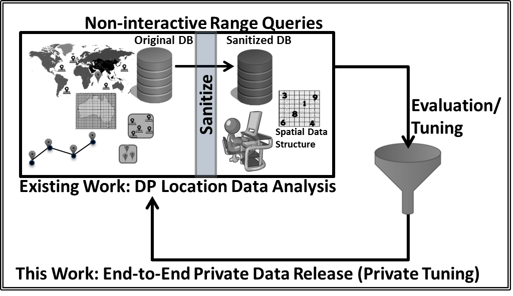
Figure 1. End-to-end private spatial data structures.

Aggregation has been used extensively for efficient range query responses, and as a strategy for qualitative privacy (Chawla et al., 2005). Differential privacy complements such approaches by addressing attacker background knowledge; to date, various spatial data structures have been adopted for private spatial data mining (Cormode et al., 2012; Chen et al., 2012; Qardaji et al., 2013b, a; He et al., 2015; Fanaeepour and Rubinstein, 2016).

As research has established that utility is highly parameter dependant (Qardaji et al., 2013b, a), parameters must be tuned on data, and therefore privately. Unfortunately, as documented recently (Hay et al., 2016), many past works on histogram release establish differential privacy of mechanisms while ignoring privacy during tuning. The DPBench framework (Hay et al., 2016) presented, articulates as an open problem the need for end-to-end privacy for truly privacy-preserving mechanisms and fair, rigorous evaluations.

In this paper, we address this problem by optimising privatised data-dependent error bounds that quantify the effect of data structure parameters. Our focus is releasing histograms, as these are the most widely used and effective spatial data structures (Qardaji et al., 2013b).

Our mechanism consists of runs over two phases: 1) among all values for the parameter, one is selected privately that is close in utility to an optimum with high probability; 2) the data structure is constructed & released privately using the selected parameter. The main challenge is bounding utility of phase two with respect to phase one’s parameter selection, and doing so privately. We consider range query relative error (Garofalakis and Gibbons, 2002; Vitter and Wang, 1999) as our objective when choosing histogram grid size. Our bounds on this error decompose into two errors, through a principled analysis: aggregation error due to the (common) use of the uniformity assumption for aggregated counts when data is non-uniformly distributed; and perturbation error due to count perturbation for phase two differential privacy.

Contributions. Our main contributions include

• For the first time, a solution to end-to-end differentially-private parameter tuning for spatial data structure release;

• A two-phase mechanism for private parameter tuning and data structure construction;

• Guarantees on differential privacy and utility;

• Extensive experimental confirmation that our mechanism is the new state-of-art for private accurate histograms.

2. Related Work

Numerous proposals have sought to address the challenge of private location-based services (Ghinita, 2013). Aggregation has widely been used as a qualitative privacy approach, by reporting aggregate numbers of objects per partition cell in response to range queries (Braz et al., 2007; Tao et al., 2004; López et al., 2005; Leonardi et al., 2014; Fanaeepour et al., 2015). Differential privacy (Dwork et al., 2006; Dwork and Roth, 2014) has also been adopted as a semantic definition for privacy when releasing structures to untrusted third parties. To achieve high utility, different variants of data structures have been explored (Qardaji et al., 2013b; Cormode et al., 2012; Chen et al., 2012; He et al., 2015; Fanaeepour and Rubinstein, 2016), such as spatial grid histograms, quad-trees, kd-trees for point locations, for trajectories, as well as user regions.

For each data structure, selection of parameters such as grid size or levels of hierarchies, is known to be of the utmost importance in affecting utility (Qardaji et al., 2013b, a; Zhang et al., 2016). The authors in (Qardaji et al., 2013b) propose Equation (1) as a guideline for selecting grid size when releasing differentially-private grid-partitioned synopses:

(1) $$m = \sqrt{\frac{N\epsilon}{c}}\enspace,$$

where $m$ is the selected grid size per direction, $N$ is the number of data points, $\epsilon$ is the total privacy budget and $c$ is a constant depending on the dataset. Their stated motivation is to balance perturbation (noise) error and aggregate (non-uniformity) error, and while they analyse each error component, their combination is performed without rigorous justification. Moreover, the authors tune $c$ on their sensitive experimental datasets, simultaneously undermining: $c$’s definition as a constant, potentially leaking privacy, and overfitting their structures to test data. We refer to this grid selection approach as Heuristic in experiments (cf. Section 8).

It has been noted that once a parameter is already tuned non-privately on past sensitive data, that parameter can be used safely on future unrelated datasets (Hay et al., 2016). However, such fixed schemes still eschew optimisation by data-dependence. Not all datasets exhibit the same levels of uniformity, point distribution or domain, as discussed in Section 5. Such approaches like Heuristic obfuscate the non-privacy of tuning $m$ by secretly tuning $c$ (or some other constant in the fixed rule). Any tuning must be privacy preserving.

The key challenge for this line of research, is that parameter selection must be data dependent but still preserve privacy. In machine learning, private hyper parameter tuning has been explored (Chaudhuri et al., 2011; Chaudhuri and Vinterbo, 2013) using cross validation. However, cross validation leverages split test & train data, as it aims to mitigate future generalisation error. Here we wish to make use of all data in all stages and are ultimately concerned with range queries against this same dataset. The two domains are related but pose fundamentally distinct challenges.

In (Li et al., 2014), a private parameter selection mechanism, for 1D data, is developed using dynamic programming. While it is speculated that the approach extends to 2D data via reducing 2D structures to 1D with space filling curves, such curves do not preserve spatial locality in general. As a result it is relatively easy to construct counter examples to such extensions.

A principled evaluation for differentially-private algorithms is reported recently in (Hay et al., 2016). The DPBench framework asserts that end-to-end privacy is quite necessary, and highlights parameter tuning as a key open problem for many existing mechanisms. We are motivated by their call, and address the problem with our end-to-end private approach for tuning and histogram construction.

3. Preliminaries and Definitions

In Table 1, summary of notations and symbols used throughout this paper are described.

Table 1. Summary of symbols used in this paper.

Symbols	Description
$D$	original dataset of points
$D^{\prime}$	neighbour dataset with $D$, differing in one record
$\mathcal{Q}$	set of query regions
t, $Q_{t}$	specification of a query region, including shape, size and position, $t\in$ $\mathcal{Q}$
$\mathcal{C}$	set of cells
$c_{i}$	count value for the $i$-th cell component, $i\in$ $\mathcal{C}$
$d_{i}$	true number of data/points in cell $i$, within $QR$, i $\in$ $\mathcal{C}$
$\alpha_{i}$	fraction of the overlapping area of $QR$ with cell $i$, $\alpha_{i}$ $\in(0,1]$
$\mathcal{G}$	set of grid sizes, $g_{r}$
$g_{r}$	size of a grid, number of divisions on each direction, $r\in\mathcal{G}$
$\rho$	sanity bound for the relative error, computed for a dataset $D$
$Y_{i}$	noise added to cell $i$
$\lambda$	scale parameter of Laplace mechanism
$\delta$	a small value in $(0,1)$, used for the sanity bound
$\epsilon,\epsilon_{1},\epsilon_{2}$	privacy parameters
$c$	constant in Heuristic approach

3.1. Spatial Data Structures

As discussed in Section 2, there is a wide range of spatial data structures (Samet, 2006) proposed for spatial object, from points, path trajectories, to planar regions (bodies). Our focus on spatial histograms derives from their wide popularity in supporting aggregate range queries. Originally developed for efficiency, histograms have found application in qualitative privacy (Tao et al., 2004; Chawla et al., 2005). Consider a dataset of points (locations), $D$, where each record is a point. Figure 2 displays a grid data structure of points (Figure 2a) and the resulting spatial histogram $\mathbf{H}$ of counts $c_{i}$ per cell $i\in\mathcal{C}$ the set of cells (Figure 2b). An aggregate range query is represented by a query region $QR$ (a red bolded rectangle in Figure 2), with corresponding responses as an approximate count of points of $D$ that fall in that query region. We apply the uniformity assumption to quantify the contribution of a cell as the cell count multiplied by the fraction of cell area in $QR$ (cf. Section 6).

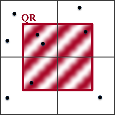
(a) Grid

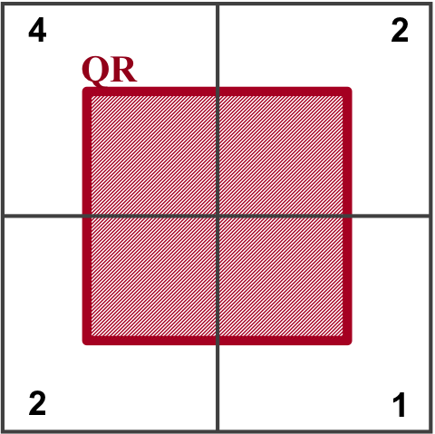
(b) Histogram

Figure 2. Points, a $2\times 2$ grid, and corresponding histogram.

3.2. Differential Privacy

We adopt the differential privacy (DP) (Dwork et al., 2006; Dwork and Roth, 2014) framework due to its strong guarantees on data privacy.

Definition 3.1.

Databases $D$ and $D^{\prime}$ that differ on exactly one record, with $D^{\prime}$ having one more than $D$, are termed neighbours.

Definition 3.2.

A randomised mechanism $\mathcal{M}$, preserves $\epsilon$-differential privacy for $\epsilon>0$, if for all neighbouring databases $D,D^{\prime}$ and measurable $S\subseteq Range(\mathcal{M})$:

$$\mathrm{Pr}(\mathcal{M}(D)\in S) \leq \exp(\epsilon)\cdot\mathrm{Pr}(\mathcal{M}(D^{\prime})\in S)\enspace.$$

Differential privacy requires that small changes to input (addition/deletion of a record) do not significantly affect a mechanism’s response distribution. As such sampling from the mechanism’s output cannot be used to distinguish the input database.

Lemma 3.3 ((Dwork et al., 2006)).

Consider mechanisms $\mathcal{M}_{i}$ each providing $\epsilon_{i}$-differential privacy, then the release of the vector of mechanism’s responses on database $D$ preserves $\sum_{i}\epsilon_{i}$-differential privacy.

Definition 3.4.

The $L_{1}$-global sensitivity (GS) of a deterministic, Euclidean-vector-valued function $f$ is given by $\Delta f=\max\limits_{D,D^{\prime}}\lVert f(D)-f(D^{\prime})\rVert_{1}$, taken over neighbouring databases.

The simplest generic mechanism for differential privacy smooths non-private function sensitivity with additive perturbations.

Theorem 3.5 ((Dwork et al., 2006)).

For any deterministic Euclidean-vector-valued $f(D)$, the Laplace mechanism $M(D)\sim Lap(f(D),\Delta f/\epsilon)$ preserves $\epsilon$-differential privacy.

Another important mechanism enables release from arbitrary sets that need not be numeric.

Theorem 3.6 ((McSherry and Talwar, 2007)).

Consider a score function (or quality, utility function) $s(D,r)\in\mathbb{R}$ for database $D$ and response $r\in\mathcal{R}$. Then the exponential mechanism that outputs response $r$ with probability

(2) $$\mathrm{Pr}(M(s,D)=r)=\frac{\exp(\epsilon\cdot s(D,r)/2\Delta)}{\sum_{r\in\mathcal{R}}\exp(\epsilon\cdot s(D,r)/2\Delta)}\enspace,$$

preserves $\epsilon$-differential privacy for $\epsilon>0$ and $\Delta=\Delta s$.

The exponential mechanism is typically used with $\Delta s=\sup_{r\in\mathcal{R}}\Delta s(\cdot,r)$. However, using response dependent sensitivity per term achieves the same privacy, with potentially better utility:

Definition 3.7.

Response-dependent sensitivity is $\Delta_{r}=\Delta s(\cdot,r)$.

4. Problem Statement

We seek to address the problem of parameter tuning spatial histograms in an end-to-end differentially-private setting (cf. Figure 1).

Problem 4.1.

Given point-set $D$, a set of query regions $\mathcal{Q}$, budget $\epsilon>0$, our goal is to batch process $D$ to produce a data structure that can respond to an unlimited number of range queries through privately selecting a grid size from given set $\mathcal{G}$ that optimises response accuracy on queries $\mathcal{Q}$, while preserving $\epsilon$-differential privacy.

4.1. Evaluation Metrics

Specifically, solutions should have the following properties:

Property 4.2 (End-to-End Differential Privacy).

Mechanisms should achieve non-interactive differential privacy not only in the release of a data structure based on spatial data but also in parameter tuning e.g., grid size selection, of the structure.

Property 4.3 (Utility: Low Relative Error).

Mechanisms should achieve low total error on future query regions $QR$, as measured by relative error $\left|response(QR)-true(QR)\right|/true(QR)$.

Property 4.4 (Efficiency: Low Computational Complexity).

Mechanisms should enjoy low computational time complexity in terms of key parameters of the data and geographic area.

Error trade-off. We expect a trade-off between two sources of error as depicted in Figure 3, illustrating the need to tune grid size: aggregation error due to failure of the uniformity assumption when aggregating for qualitative privacy; perturbation error due to count noise introduced for differential privacy.

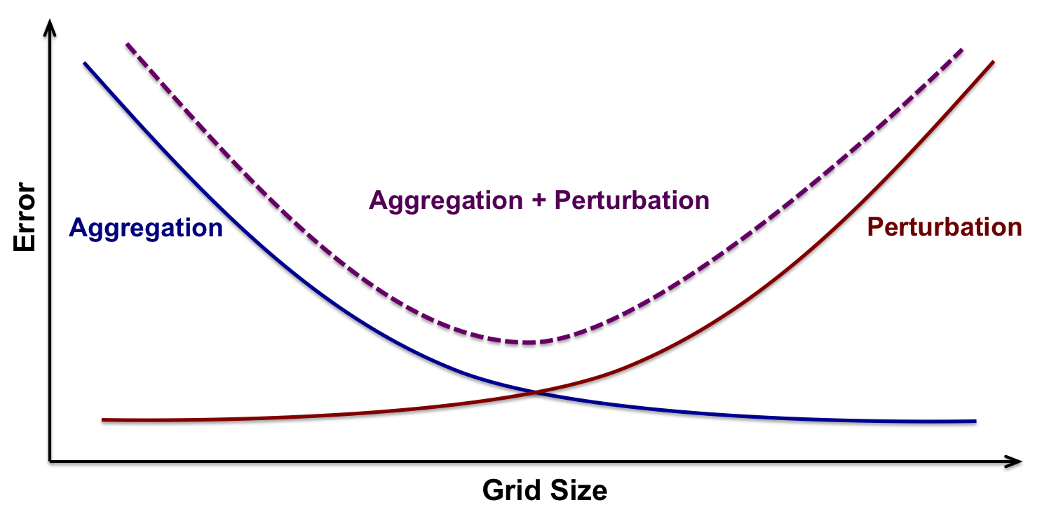
Figure 3. Expected error trade-off, demonstrating that optimal grid size depends on the combination of error sources.

5. Commentary on Heuristic Approach

Qardaji et al. (Qardaji et al., 2013b) propose the Heuristic grid size selection approach as the fixed-rule Equation (1). An idealisation of the kind of situation in which Heuristic fails is presented in Figure 4. Heuristic might suggest a $4\times 4$ grid here (Figure 4a) based on the number of points and assuming uniformity. However, a $QR$ that happens to be located over regions of non-uniformity—precisely where the uniformity assumption fails–leads to erroneous query response. For concreteness, if the four well-populated cells contain 100 points each (with just 1 each within the $QR$), then the response on the $QR$ would be 100: each cell contributes $100\cdot 0.25$. By contrast, on an alternate $8\times 8$ partitioning (Figure 4b), the response to the same $QR$ would be the correct count of $4$. In this case, the uniformity assumption and $QR$ align perfectly. Heuristic is derived with reliance on the uniformity assumption, and is incapable of adapting to datasets where it holds to a greater/lesser degree.

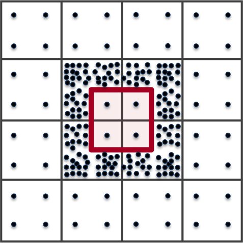
(a) $4\times 4$ grid

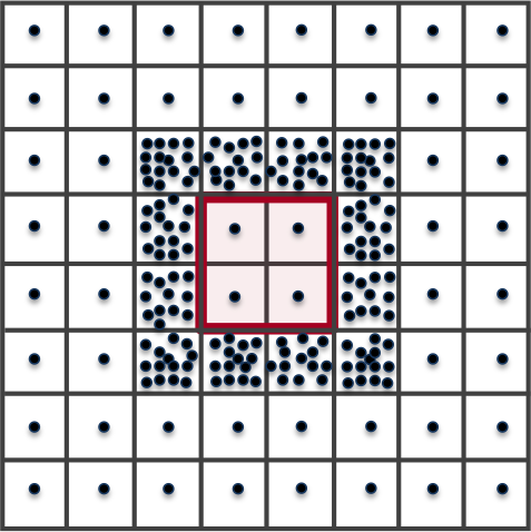
(b) $8\times 8$ grid

Figure 4. The bolded red rectangle depicts the Query Region ($QR$), dots illustrate points. The non-uniformly located points across the $QR$ boundary resulting in erroneous count using uniformity assumption for a $4\times 4$ grid.

While the derivation of Heuristic considers both error sources separately, the combination of bounds is not justified. Our approach privately optimises a rigorously-derived bound on total error.

Finally, the recommendation c$=10$ is determined not on unrelated datasets, but openly optimised utility on the evaluation datasets. Not only does this practice violate differential privacy (Hay et al., 2016) but it fails to guarantee good utility when applied to future datasets.

Motivated by the expected need for balancing errors through data-dependent grid tuning (cf. Figure 3), we explore utility vs. grid size under the Storage dataset for fixed $QR$ of 1% of domain size (cf. Section 8 for dataset details). This dataset was used in the non-private tuning of $c$ in Heuristic in (Qardaji et al., 2013b). While the results of the tuning where not compared with the true optimum, we make this comparison in Figure 5. The trade-off between errors is as predicted (Figure 3). Moreover the grid chosen by Heuristic is far from optimal, further confirming that fixed parameters are unsuitable for accurate responses, and that private data-dependent tuning is needed.

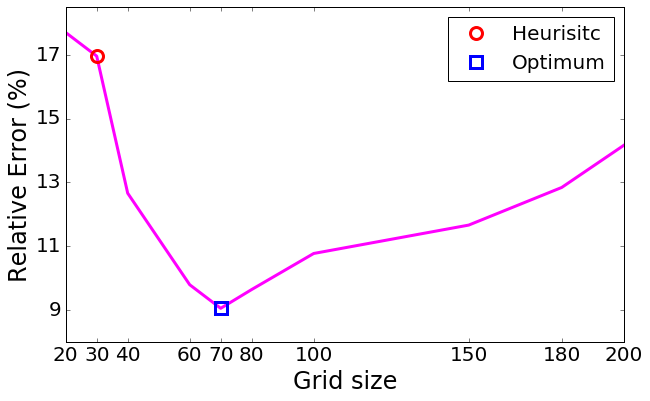
Figure 5. Effect of grid size on response utility for Storage dataset, demonstrating selection must be data dependent.

6. Approach: E2EPriv

Our solution to end-to-end $\epsilon$-differentially-private histogram release, E2EPriv, consists of two phases with budgets $\epsilon_{1}+\epsilon_{2}=\epsilon$: 1) Select one from a set of given grid sizes, by privately minimising data-dependent expected error bounds on a given set of $QR$s; 2) Construct a histogram with chosen grid size, privatized by perturbing cell counts. Algorithm 1 (Section 6.1) describes these phases and the process of responding to subsequent queries using the released data structure is described by Algorithm 2 (Section 6.2).

6.1. Spatial Histograms Release

Consider Algorithm 1, which releases a tuned spatial histogram. In Phase 1 [lines 1–1], a histogram $\mathbf{H}$ is constructed on $D$, for each candidate grid size in $\mathcal{G}$. In Phase 2, cell counts will be privatized by adding Laplace-distributed r.v. $Y_{i}$ to count $i$ as

(3) $$Y_{i}\sim Lap(0;\lambda)\ ,\ \ \ Var(Y_{i})=2\lambda^{2}\ ,\ \ \ \mathbb{E}\left[\left|Y_{i}\right|\right]=\lambda\enspace,$$

taking $\lambda=1/\epsilon_{2}$. The idea behind the algorithm is to compute a bound on the expected relative error that this (future) noisy histogram would incur, averaged over the $QR$s in $\mathcal{Q}$, as evaluated on the data $D$. The bound’s expression (Corollary 7.6) involves comparing the histogram $\mathbf{H}$ response on each $QR$ with the true count on $QR$, and then to the absolute of this quantity (reflecting aggregation error) the expected perturbation (3).

Note that histogram response to $QR$ involving the uniformity assumption requires computation of the area overlap between each cell $i$ in $\mathbf{H}$ and the $QR$,

(4) $$\alpha_{i}=\frac{Area(QR\cap cell_{i})}{Area(cell_{i})}\in[0,1],\enspace i\in\mathcal{C}\enspace.$$

Input : Dataset of points $D$; Set of grid sizes $\mathcal{G}$; Set of range queries $\mathcal{Q}$; Privacy budgets $\epsilon_{1},\epsilon_{2}$

Output : Selected grid size $g^{\star}$; Histogram $\mathbf{H^{\prime}}$

1 Phase 1: Privately tune the grid cell size:

2for $g\in\mathcal{G}$ do

3      

4      Initialise histogram $\mathbf{H}$ of counts per cell (each sized $g$).

5      for $p\in D$ do

6             Increment the count of $\mathbf{H}$’s cell that $p$ falls in.

7      

8      for $QR\in\mathcal{Q}$ do

9             Compute overlap $\alpha_{i}$ between $QR$ & each cell $i$ in $\mathbf{H}$.

10            Compute $\mathbf{H}$’s non-private $QR$ response $response(QR)=\sum_{i}\alpha_{i}\cdot c_{i}$.

11            Count $true(QR)$ number points in $D$ falling in $QR$.

12            Compute $error(QR)$ bound as per Corollary 7.6

13      Compute average error bound $avgError$ over $\mathcal{Q}$.

14      Set exponential mechanism score $s(D,g)=-avgError$.

15      Compute the probability of responding $g$, using privacy parameter $\epsilon_{1}$, as Equation (2)

16      Compute bound/score sensitivity $\Delta_{g}$ from Corollary 7.9.

17Sample $g^{\star}$ as $r$ w.p. $\propto\exp(\epsilon_{1}\cdot s(D,r)/2\Delta_{r})$.

18Phase 2: Construct the private histogram counts:

19Re-create the histogram $\mathbf{H}$ for chosen grid size $g^{\star}$.

20Perturb the cell counts with iid Laplace noise per cell, $\mathbf{H^{\prime}}=\mathbf{H}+\mathbf{Y}$, $\mathbf{Y}\sim Lap(0;\lambda),\lambda=1/\epsilon_{2}$.

21

Algorithm 1 End-to-End Differentially Private Spatial Histogram Construction via Private Grid Size Tuning

To minimise averaged error bound (over each query in $\mathcal{Q}$) we set the exponential mechanism’s score function (cf. Theorem 3.6) for maximisation to be the negative error. To calibrate the mechanism, we use the sensitivity of this score function as bounded in Corollary 7.9. Detailed derivation of these bounds is provided in Section 7. The result is a sampled $g^{\star}$ which approximates the grid size optimising the (data-dependent non-private) error bound.

In Phase 2 [lines 1–1], a private histogram is produced for the chosen grid size $g^{\star}$ using the Laplace mechanism—following the same process as simulated in Phase 1.

Computational Complexity. Algorithm 1 is efficient with time complexity $O(\lvert D\rvert\cdot\lvert\mathcal{Q}\rvert\cdot\lvert\mathcal{G}\rvert\cdot g^{2})$ and space complexity $O(\lvert\mathcal{G}\rvert+g^{2})$. The parameter $g$ is the largest grid size in $\mathcal{G}$: it is necessary to touch at least every cell.

6.1.1. Computing cell, $QR$ overlap

Figure 6 illustrates an example $QR$ intersecting with a histogram cells.

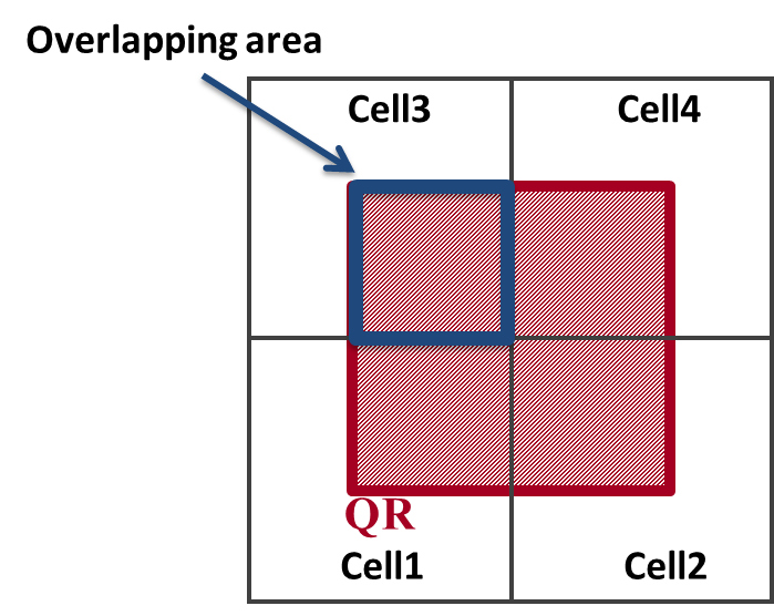
Figure 6. A query region, $QR$, intersecting with grid cells and its overlapping area of a cell.

To compute the fraction $\alpha_{i}$ of overlapping area of a $QR$ with a cell $i$ as defined in Equation (4), we have the special case of polygon intersection from computational geometry (O’Rourke, 1998)

$$Area(QR\cap cell_{i})=x_{overlap}\times y_{overlap}$$

where

$$x_{overlap} = \max(0,\min(x_{12},x_{22})-\max(x_{11},x_{21}))$$

$$y_{overlap} = \max(0,\min(y_{12},y_{22})-\max(y_{11},y_{21}))$$

cell coordinates $$= [(x_{11},y_{11}),(x_{12},y_{12})]\enspace,$$

$$QR = [(x_{21},y_{21}),(x_{22},y_{22})]\enspace.$$ coordinates

Note that $\sum_{i\in\mathcal{C}}\lceil\alpha_{i}\rceil\equiv\mbox{ \# overlapping cells}$.

6.2. Post-Release Range Query Response

Input : Histogram $\mathbf{H}$ with cells $\mathcal{C}$; Query $QR$

Output : Approximate count $response(QR)$

1

2for $i\in\mathcal{C}$ do

3       Compute overlap $\alpha_{i}$ of $i$ with $QR$, using Equation (4).

4      Compute cell’s contribute $z_{i}=\alpha_{i}\cdot c_{i}$.

5Sum the contributions $response(QR)=\sum_{i\in\mathcal{C}}z_{i}$.

Algorithm 2 Range Query Response

Algorithm 2 takes histogram $\mathbf{H}$, query $QR$, to a response. The algorithm simply weighs each cell’s count by its overlap $\alpha_{i}$ with the $QR$, applying the uniformity assumption.

Computational Complexity. The range query algorithm is efficient in time $O(g^{2})$ linear in the number of cells & constant space.

7. Theoretical Analysis

Having described key concepts underlying Algorithm 1 in the previous section, we now derive the bound on expected error of Phase 2’s histogram release (Corollary 7.6), that is privately minimised by the mechanism; we prove differential privacy (Theorem 7.10) and provide a utility bound (Theorem 7.11). A key component of our analysis is in bounding sensitivity of our error bound to perturbations in the input dataset (Corollary 7.9). By using a more refined response-dependent sensitivity our mechanism enjoys improved utility at no price to privacy (cf. Section 8.8 for a discussion).

We begin our analysis for the single tuning query case (Section 7.1, and then extend to multiple queries (Section 7.2).

7.1. Case: Single Tuning Query

We first bound expected error of Phase 2 when responding to a single (tuning) $QR$. We bound both absolute error, and relative error. We introduce a constant $\rho$ in the denominator of the latter in order to control sensitivity in Theorem 7.5, as discussed in Remark 7.3.

Theorem 7.1.

For any given query region $QR$, the histogram $\mathbf{H^{\prime}}$ released by Algorithm 1 Phase 2 on data $D$ achieves expected error (wrt randomness in the $Y_{i}$) bounded as,

1. Absolute error:

   $$\mathbb{E}\left[\left|response\left(QR\right)-true\left(QR\right)\right|\right] \leq \left|\sum_{i\in\mathcal{C}}\alpha_{i}c_{i}-\sum_{i\in\mathcal{C}}d_{i}\right|+\lambda\lVert\bm{\alpha}\rVert_{1}.$$

2. Relative error:

   $$\mathbb{E}\left[\frac{\left|response(QR)-true(QR)\right|}{\max\{true(QR),\rho\}}\right]\leq\frac{\left|\sum_{i\in\mathcal{C}}\alpha_{i}c_{i}-\sum_{i\in\mathcal{C}}d_{i}\right|+\lambda\lVert\bm{\alpha}\rVert_{1}}{\max\{\sum_{i\in\mathcal{C}}d_{i},\rho\}}.$$

where $\rho>1$ is a constant (cf. Remark 7.3), and $d_{i}$ counts the number of points in $D$ falling in both cell $i$ and $QR$.

Proof.

Consider the first case of absolute error,

$$\mathbb{E}\left[\left|\sum_{i\in\mathcal{C}}\alpha_{i}(c_{i}+Y_{i})-\sum_{i\in\mathcal{C}}d_{i}\right|\right]$$

$$\leq \mathbb{E}\left[\left|\sum_{i\in\mathcal{C}}\alpha_{i}c_{i}-\sum_{i\in\mathcal{C}}d_{i}\right|\right]+\mathbb{E}\left[\left|\sum_{i\in\mathcal{C}}\alpha_{i}Y_{i}\right|\right]$$

$$\leq \left|\sum_{i\in\mathcal{C}}\alpha_{i}c_{i}-\sum_{i\in\mathcal{C}}d_{i}\right|+\lambda\lVert\bm{\alpha}\rVert_{1}\enspace,$$

where the first inequality follows from rearranging terms and applying the triangle inequality and monotonicity & linearity of expectation; the second inequality follows from the same arguments combined with Equation (3):

$$\mathbb{E}\left[\left|\bm{\alpha}\cdot\mathbf{Y}\right|\right]\ \ \leq\ \ \sum_{i\in\mathcal{C}}\alpha_{i}\mathbb{E}\left[\left|Y_{i}\right|\right]\ \ =\ \ \lambda\lVert\bm{\alpha}\rVert_{1}\enspace.$$

The second claim follows immediately. ∎

Remark 7.2.

It is notable that the bound decomposes total (expected) error into two interpretable terms: $\left|\sum_{i\in\mathcal{C}}\alpha_{i}c_{i}-\sum_{i\in\mathcal{C}}d_{i}\right|$ reflecting aggregation error due to spatial aggregation and (potential) failure of the uniformity assumption; and $\lambda\|\bm{\alpha}\|_{1}$ reflecting error due to random perturbation from the Laplace mechanism, where $\lambda$ is noise scale and $\|\bm{\alpha}\|_{1}$ counts the (effective) cells overlapping the $QR$.

Remark 7.3.

$\rho>1$ is a user-defined constant, referred to as the sanity bound in the literature (Garofalakis and Gibbons, 2002; Vitter and Wang, 1999). It is commonly used to control sensitivity of relative error measures in the face of small true counts that can potentially yield unbounded blow-up of relative error. Previous recommendations set it as $\rho=\delta\times|D|$, where $0<\delta<1$ is taken to be a small constant reflecting a pseudo-count fraction of $D$.

As Algorithm 1 Phase 1 privately minimises the relative the error bound on Phase 2 of Theorem 7.1—using the exponential mechanism—we must compute the sensitivity of this bound which itself is data-dependent and hence privacy-sensitive. We cannot simply optimise the error bound of Theorem 7.1 directly, as implicitly done by Heuristic, lest we breach data privacy.

We define the exponential mechanism’s score (quality) function as the negative relative error bound: maximising this score over candidate grid sizes $\mathcal{G}$, equivalently minimised the error bound, which in turn is a close surrogate for minimising actual future error of Phase 2 on the tuning query set $\mathcal{Q}$.

(5) $$s(D,r) = -\frac{\left|\sum_{i\in\mathcal{C}}\alpha_{i}c_{i}-\sum_{i\in\mathcal{C}}d_{i}\right|+\lambda\lVert\bm{\alpha}\rVert_{1}}{\max\{\sum_{i\in\mathcal{C}}d_{i},\rho\}}\enspace.$$

And we make the analogous definition if optimising absolute error:

$$s(D,r) = -\left|\sum_{i\in\mathcal{C}}\alpha_{i}c_{i}-\sum_{i\in\mathcal{C}}d_{i}\right|-\lambda\lVert\bm{\alpha}\rVert_{1}\enspace.$$

To calibrate the exponential mechanism for differential privacy, we must bound the sensitivity $\Delta s$ of the score function.

Lemma 7.4.

The global sensitivity of the absolute score function, is bounded above by $\left|1-\alpha_{i}\right|$ which is at most $1$, as each $\alpha_{i}\in(0,1]$.

Proof.

From the reverse triangle inequality we have

$$GS(s)=\Delta=\max_{r,\lVert D-D^{\prime}\rVert_{1}\leq 1}\lvert s(D,r)-s(D^{\prime},r)\rvert$$

$$\leq \left|\left(\left|\sum_{i\in\mathcal{C}}\alpha_{i}c_{i}-\sum_{i\in\mathcal{C}}d_{i}\right|+\lambda\lVert\bm{\alpha}\rVert_{1}\right)-\left(\left|\sum_{i\in\mathcal{C}}\alpha_{i}c^{\prime}_{i}-\sum_{i\in\mathcal{C}}d^{\prime}_{i}\right|+\lambda\lVert\bm{\alpha}\rVert_{1}\right)\right|$$

$$\leq \lvert\lvert\alpha_{1}c_{1}+\alpha_{2}c_{2}+\dots+\alpha_{i}c_{i}+\dots-(d_{1}+d_{2}+\dots+d_{i}+\dots)\rvert-$$

$$\lvert\alpha_{1}c_{1}+\alpha_{2}c_{2}+\dots+\alpha_{i}(c_{i}+1)+\dots$$

$$-(d_{1}+d_{2}+\dots+d_{i}+1+\dots)\rvert\rvert$$

$$\leq \lvert\lvert\alpha_{1}c_{1}+\alpha_{2}c_{2}+\dots+\alpha_{i}c_{i}+\dots-(d_{1}+d_{2}+\dots+d_{i}+\dots)\rvert$$

$$-\lvert\big{(}\alpha_{1}c_{1}+\alpha_{2}c_{2}+\dots+\alpha_{i}c_{i}+\dots-(d_{1}+d_{2}+\dots+d_{i}+\dots)\big{)}$$

$$+(\alpha_{i}-1)\rvert\rvert$$

$$= \left|1-\alpha_{i}\right|\enspace.$$

∎

The case for relative error is much more involved.

Theorem 7.5.

The response-dependent sensitivity of relative error score function (5), for any $r\in\mathcal{G}$ and fixed query $t\in\mathcal{Q}$, is bounded

$$\Delta_{r}s \leq \frac{1}{\delta(\delta\left|D\right|+1)}+\frac{\lambda\lVert\bm{\alpha}^{r}\rVert_{1}}{\delta\left|D\right|(\delta\left|D\right|+1)}+\frac{1}{\delta\left|D\right|+\delta}\enspace,$$

where $\delta\in(0,1)$ defines sanity bound constant $\rho=\delta\left|D\right|$. We introduce superscript $r$ to $\bm{\alpha}$, to highlight explicit dependence on $r\in\mathcal{G}$.

To prove the result we must bound the quantity

$$\left|\frac{1}{\max\{\sum_{i\in\mathcal{C}}d_{i},\rho\}}\left(\left|\sum_{i\in\mathcal{C}}\alpha_{i}c_{i}-\sum_{i\in\mathcal{C}}d_{i}\right|+\lambda\lVert\bm{\alpha}\rVert_{1}\right)-\right.$$

$$\left.\frac{1}{\max\{\sum_{i\in\mathcal{C}}d^{\prime}_{i},\rho^{\prime}\}}\left(\left|\sum_{i\in\mathcal{C}}\alpha_{i}c^{\prime}_{i}-\sum_{i\in\mathcal{C}}d^{\prime}_{i}\right|+\lambda\lVert\bm{\alpha}\rVert_{1}\right)\right|\enspace,$$

where $\rho=\delta\times\left|D\right|$ and $\rho^{\prime}=\delta\times\left|D^{\prime}\right|=\delta\times(\left|D\right|+1)=\rho+\delta$. The proof proceeds by cases, based on where $D^{\prime}$’s extra point falls: outside $QR$ and cells overlapping $QR$ (Figure 7a); outside $QR$, inside cells overlapping $QR$ (Figure 7b); or inside $QR$ (Figure 7c). The reader interested in the (technical) calculations for the full proof of the theorem are referred to Appendix A.

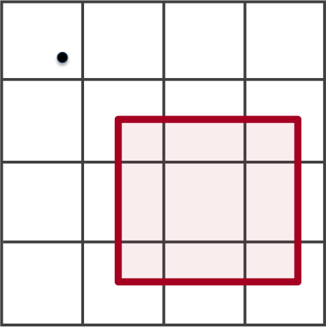
(a) Case 1.

(b) Case 2.

(c) Case 3.

Figure 7. Cases in the proof of Theorem 7.5 based on where the extra point (dot) falls relative to the $QR$ (red) and cells overlapping the $QR$ (the bottom right $3\times 3$ cells).

7.2. Case: Multiple Tuning Queries

Before proceeding to privacy and utility guarantees, we lift the above single query analysis, to the case of multiple tuning queries. The first step is bounding average Phase 2 error over query set $\mathcal{Q}$. This follows from Theorem 7.1 and linearity of expectation.

Corollary 7.6.

For given set of query region $\mathcal{Q}$, the histogram $\mathbf{H^{\prime}}$ released by Algorithm 1 Phase 2 on data $D$ achieves average expected error (wrt randomness in the $Y_{i}$) bounded as,

1. Absolute error:

   $$\mathbb{E}\left[\frac{1}{|\mathcal{Q}|}\sum_{t\in\mathcal{Q}}\left|response\left(t\right)-true\left(t\right)\right|\right]$$

   $$\leq \frac{1}{|\mathcal{Q}|}\sum_{t\in\mathcal{Q}}\left(\left|\sum_{i\in\mathcal{C}}\alpha_{i}^{t}c_{i}-\sum_{i\in\mathcal{C}}d_{i}\right|+\lambda\lVert\bm{\alpha}^{t}\rVert_{1}\right)\enspace.$$

2. Relative error:

   $$\mathbb{E}\left[\frac{1}{|\mathcal{Q}|}\sum_{t\in\mathcal{Q}}\frac{\left|response(t)-true(t)\right|}{\max\{true(t),\rho\}}\right]$$

   $$\leq \frac{1}{|\mathcal{Q}|}\sum_{t\in\mathcal{Q}}\frac{\left|\sum_{i\in\mathcal{C}}\alpha_{i}^{t}c_{i}-\sum_{i\in\mathcal{C}}d_{i}\right|+\lambda\lVert\bm{\alpha}^{t}\rVert_{1}}{\max\left\{\sum_{i\in\mathcal{C}}d_{i},\rho\right\}}\enspace.$$

where $\rho>1$ is a constant (cf. Remark 7.3), $d_{i}$ counts the number of points in $D$ falling in both cell $i$ and $QR$ $t$, and $\bm{\alpha}^{t}$ denotes the vector of cell overlaps with $t$.

For the general case, we therefore define the exponential mechanism’s score function as before, as the negative of the bound on the expectation of the error averaged over $\mathcal{Q}$,

(6) $$s(D,r) = -\frac{1}{|\mathcal{Q}|}\sum_{t\in\mathcal{Q}}\frac{\left|\sum_{i\in\mathcal{C}}\alpha_{i}^{t}c_{i}-\sum_{i\in\mathcal{C}}d_{i}\right|+\lambda\lVert\bm{\alpha}^{t}\rVert_{1}}{\max\{\sum_{i\in\mathcal{C}}d_{i},\rho\}}\enspace.$$

And again we make the analogous definition if optimising absolute error:

$$s(D,r) = -\frac{1}{|\mathcal{Q}|}\sum_{t\in\mathcal{Q}}\left(\left|\sum_{i\in\mathcal{C}}\alpha_{i}^{t}c_{i}-\sum_{i\in\mathcal{C}}d_{i}\right|+\lambda\lVert\bm{\alpha}^{t}\rVert_{1}\right)\enspace.$$

We next extend the calculation of response-dependent sensitivity of this bound to perturbations of the database $D$.

Lemma 7.7.

For $i\in\mathcal{I}$ a finite index set, functions $f_{i}:\mathcal{X}\to\mathbb{R}$ on arbitrary domain, and constants $\Delta_{i}\in\mathbb{R}$,

$$\left(\forall i\in\mathcal{I},\sup_{x\in\mathcal{X}}|f_{i}(x)|\leq\Delta_{i}\right) \Rightarrow \sup_{x\in\mathcal{X}}\left|\frac{1}{|\mathcal{I}|}\sum_{i\in\mathcal{I}}f_{i}(x)\right|\leq\frac{1}{|\mathcal{I}|}\sum_{i\in\mathcal{I}}\Delta_{i}$$

Proof.

Applying the triangle inequality and distributing the supremum yields the result,

$$\sup_{x\in\mathcal{X}}\left|\frac{1}{|\mathcal{I}|}\sum_{i\in\mathcal{I}}f_{i}(x)\right| \leq \sup_{x\in\mathcal{X}}\frac{1}{|\mathcal{I}|}\sum_{i\in\mathcal{I}}|f_{i}(x)|$$

$$\leq \frac{1}{|\mathcal{I}|}\sum_{i\in\mathcal{I}}\sup_{x\in\mathcal{X}}|f_{i}(x)|$$

$$\leq \frac{1}{|\mathcal{I}|}\sum_{i\in\mathcal{I}}\Delta_{i}\enspace.$$

∎

Corollary 7.8.

The response-dependent sensitivity of averaged absolute error score function over query set $\mathcal{Q}$, for any $r\in\mathcal{G}$, is bounded by $1$.

Proof.

The claim bounds sensitivity of the absolute error score function derived from the averaged error bound of Corollary 7.6. The result follows immediately from Lemma 7.7 by taking: functions $f_{i}$ as the sensitivities of the individual $QR$-specific score functions; and the $\Delta_{i}$ bounds on each $f_{i}$ as the single-query sensitivity bound from Lemma 7.4. ∎

Corollary 7.9.

The response-dependent sensitivity of averaged relative error score function (6) over query set $\mathcal{Q}$, for any $r\in\mathcal{G}$, is bounded

$$\Delta_{r}s \leq \frac{1}{\delta(\delta\left|D\right|+1)}+\frac{(\lambda/|\mathcal{Q}|)\sum_{t\in\mathcal{Q}}\lVert\bm{\alpha}^{r,t}\rVert_{1}}{\delta\left|D\right|(\delta\left|D\right|+1)}+\frac{1}{\delta\left|D\right|+\delta}\enspace,$$

where $\delta\in(0,1)$ defines sanity bound constant $\rho=\delta\left|D\right|$. We introduce superscripts $r,t$ to $\bm{\alpha}$, to highlight explicit dependence on $r\in\mathcal{G},t\in\mathcal{Q}$.

Proof.

The claim bounds sensitivity of the score function (6) derived from the averaged error bound of Corollary 7.6. The result follows immediately from Lemma 7.7 by taking: functions $f_{i}$ as the sensitivities of the individual $QR$-specific score functions; and the $\Delta_{i}$ bounds on each $f_{i}$ as the single-query sensitivity bound from Theorem 7.5. ∎

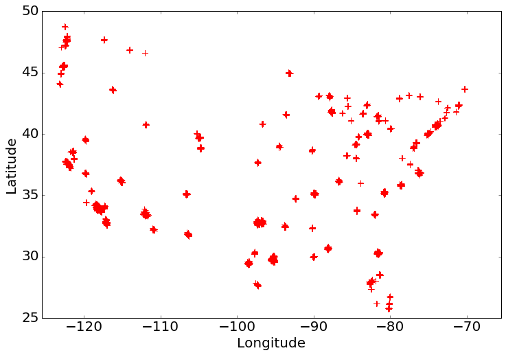
(a) Storage, with $8,938$ points.

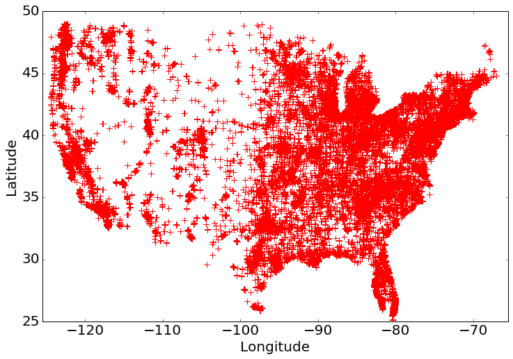
(b) Landmark, with $869,976$ points.

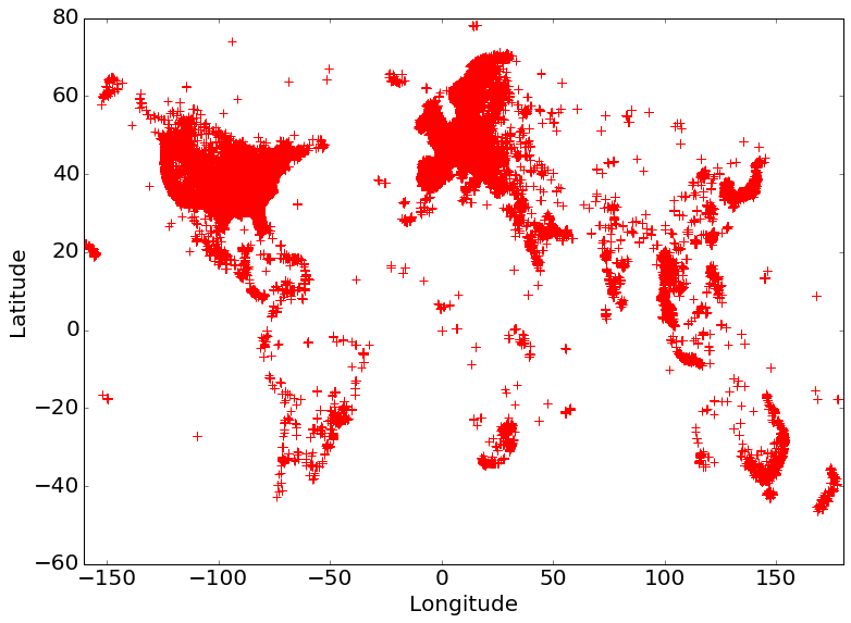
(c) Gowalla Check-ins, with $6,442,841$ points.

Figure 8. Visualising the experimental datasets.

7.3. Main Results: Privacy & Utility Guarantees

With the Phase 2 error bounds and sensitivity of these bounds in hand, we are able to present general guarantees for the end-to-end Algorithm 1.

Table 2. Experimental settings. This table demonstrates the range of parameters, bolded are those that are varying.

Dataset, Size	Grid Size (g)	$\delta$	Sanity Bound, $\rho=\delta\cdot\lvert D\rvert$	$QR$ Size (%)	Privacy Budget, $\epsilon$	$\epsilon_{1}$ (% of $\epsilon$)
Storage, 8,938 points	30, 40, 50, 60, 70, 80	0.1	893.8	1, 4, 9, 16, 25, 64	1	20
Landmark, 869,976 points	200, 250, 300, 350, 400	0.1	869,9.76	1, 4, 9, 16, 25, 64	1	20
Gowalla, 6,442,841 points	300, 400, 500, 600, 700, 800	0.1	6,442.841	1, 4, 9, 16, 25, 64	1	20
Storage, 8,938 points	40, 60, 80	0.002, 0.001, 0.1	17.88, 89.38, 893.8	1, 4, 9, 16, 25, 64	1	20
Storage, 8,938 points	30, 40, 50, 60, 70, 80	0.1	893.8	1	0.2,0.4,0.6, 0.8, 1	20
Storage, 8,938 points	30, 40, 50, 60, 70, 80	0.1	893.8	1, 4, 9, 16, 25, 64	1	20, 25, 50, 75

Theorem 7.10.

Algorithm 1 preserves $(\epsilon_{1}+\epsilon_{2})$-differential privacy.

Proof.

Phase 1 of the algorithm corresponds to the exponential mechanism, in that its release is sampled according to the exponential mechanism’s response distribution, using the score function (6). Since the algorithm uses response-dependent sensitivity $\Delta_{r}$ as bounded in Corollary 7.9 with privacy parameter $\epsilon_{1}$, it preserves $\epsilon_{1}$-differential privacy by Theorem 3.6. Phase 2 uses the resulting sanitized $g^{\star}$ which expends no further privacy budget, but runs the Laplace mechanism with sensitivity 1 (global sensitivity for histogram release) with privacy parameter $\epsilon_{2}$. By Theorem 3.5 the second phase therefore preserves $\epsilon_{2}$-differential privacy. Finally by sequential composition Lemma 3.3, the algorithm in total preserves differential privacy at level $\epsilon_{1}+\epsilon_{2}$. ∎

Our utility guarantee follows from our careful choice of score function, as itself a bound on algorithm error, combined with utility of the exponential mechanism (McSherry and Talwar, 2007; Dwork and Roth, 2014).

Theorem 7.11.

Let $\mathcal{G}_{OPT}=\{r\in\mathcal{G}:s(D,r)=OPT_{s}(D)\}$ be the set of truly optimising grid sizes—i.e., each achieves the maximum score of all $\mathcal{G}$ grid sizes $OPT_{s}(D)=\max_{r\in\mathcal{G}}s(D,r)$; and let $g^{\star}$ be the output of Algorithm 1. Then for all $\tau>0$

$$\Pr\left[s(g^{\star})\leq OPT_{s}(D)-\frac{2\Delta}{\epsilon_{1}}\left(log\left(\frac{\lvert\mathcal{G}\rvert}{\lvert\mathcal{G}_{OPT}\rvert}\right)+\tau\right)\right] \leq e^{-\tau}\enspace,$$

where $\Delta=\max_{r\in\mathcal{G}}\Delta_{r}$, each as defined in Corollary 7.9.

With high probability the selected $g^{\star}\in\mathcal{G}$ has a score close to $OPT_{s}(D)$ by more than an additive factor of $O((\Delta/\epsilon_{1})\log\lvert\mathcal{G}\rvert)$ (McSherry and Talwar, 2007; Dwork and Roth, 2014) i.e., the error has only logarithmic dependence on $\lvert\mathcal{G}\rvert$. Notably the bound depends on $\epsilon_{2}$ (in addition to $\epsilon_{1}$), through $\Delta$.

7.4. Discussion of Sensitivity Bound

Conventionally the exponential mechanism is used with a global bound on score/quality function sensitivity $\Delta$, so as to be independent of response. Following this approach yields two alternative, potentially more conveniently implemented, sensitivity bounds of

(7) $$\frac{1}{\delta(\delta\left|D\right|+1)}+\frac{\frac{\lambda}{\left|\mathcal{Q}\right|}\sum_{t\in\mathcal{Q}}\max_{r}\lVert\bm{\alpha}^{r,t}\rVert_{1}}{\delta\left|D\right|(\delta\left|D\right|+1)}+\frac{1}{\delta\left|D\right|+\delta}$$

(8) $$\leq \frac{1}{\delta(\delta\left|D\right|+1)}+\frac{\lambda\max\{g^{2}\}}{\delta\left|D\right|(\delta\left|D\right|+1)}+\frac{1}{\delta\left|D\right|+\delta}\enspace,$$

where the first bound has removed dependence on grid size by simply maximising over grid size in the single-query sensitivity bound, then averaging. The second sensitivity bound follows from the observation that the $\|\bm{\alpha}^{r,t}\|_{1}$ terms each quantify the effective number of cells overlapped by the $QR$ $t$, which cannot be any larger than the total number of cells in the histogram. This in turn is maximised by the grid size with largest number of cells. Figure 9 shows that maximising over the grid sizes per $QR$, will always yield the largest grid size.

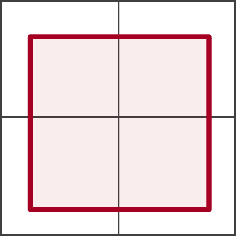
(a) $2\times 2$ grid

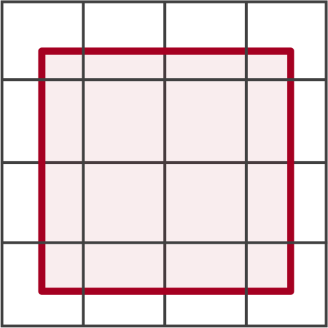
(b) $4\times 4$ grid

Figure 9. Maximising over grid sizes, will be always the largest one.

Both of these alternative approaches would be natural to use with the exponential mechanism, as response-independent global sensitivities. However, they are both upper-bounds on our response-dependent sensitivity and as such can lead to lower utility. We demonstrate this effect experimentally in Section 8.8.

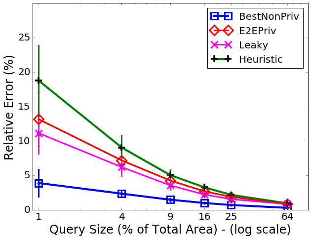
(a) Storage dataset.

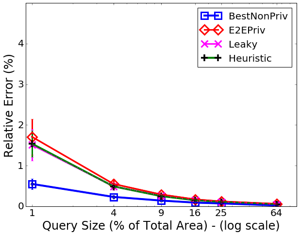
(b) Landmark dataset.

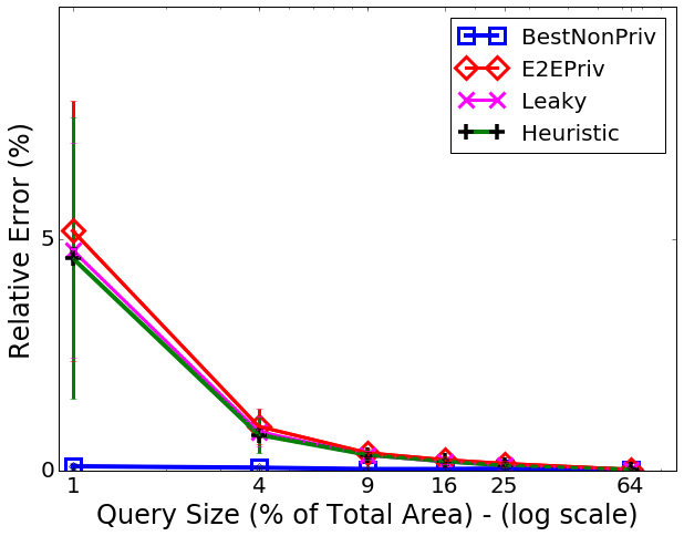
(c) Gowalla Check-ins dataset.

Figure 10. Effect of QR size (% of total area) in performance; computing median relative error per query size.

8. Experimental Study

We now describe our comprehensive experimental study.

8.1. Baselines

We employ three baselines mechanisms in our comprehensive evaluation. Compared to our truly end-to-end private approach, these approaches are either partially private or not differentially private on new datasets.

Heuristic (Qardaji et al., 2013b) computes grid size via Equation (1), as described in Sections 2 and 5. The authors select $c=10$ based on tuning to the datasets used here. We expect privacy only when $c$ is not tuned, and as argued, it is not adaptive to the underlying data, but is based on (partly) principled derivation.

Leaky is a semi-private approach, tuning grid size by adding noise to the original histogram counts (privately) but then comparing different grid sizes on sensitive data non-privately. The entire privacy budget is allocated to the histogram release, none to (non-private) tuning.

BestNonPriv non-privately releases the unpertrubed histogram. Without considering noise, tuning optimizes aggregate error alone, and so always chooses the largest grid size.

8.2. Datasets

We run experiments on three datasets—Storage, Landmark, Gowalla Check-ins—ranging in size, uniformity and sparsity as visualised in Figure 8. These datasets were used in (Qardaji et al., 2013b) to evaluate and in fact tune Heuristic (finding $c=10$). In this way, we deliver Heuristic a significant advantage, providing a fair and comprehensive comparison between our mechanism and the baselines.

Two datasets are in the USA. The first dataset, Storage 8a, consists of US storage facility locations composed of national chain storage facilities in addition to locally owned and operated facilities. This is a small dataset of 8,938 points. Geographical coordinates range over (-125.5, -65.5) and (25.0, 50.0) for longitude and latitude respectively. Geographical distances are 60 for Lon axis and 25 for Lat axis. The distance in metres for the x axis is $\approx$6000$Km$, and for y axis is $\approx$2800$km$. The second dataset, Landmark Figure 8b, is a large dataset of 869,976 points. This is a dataset of locations of landmarks in the 48 US continental states. The listed landmarks range from schools and post offices to shopping centres, correctional facilities, and train stations from the 2010 Census TIGER point landmarks. As indicated in (Qardaji et al., 2013b), this dataset appears to match the population distribution in the USA. In terms of domain specification, size, longitude and latitude ranges, the dataset is identical to Storage.

The third and final dataset is the check-in dataset obtained from the Gowalla location-based social network, where users share their locations by checking in. This dataset has the time and location information of check-ins made by users over the period of February 2009–October 2010. For the purpose of this experiment only the location information has been used. This dataset consists of 6,442,841 points, making it a large-sized dataset spanning the entire world map, Figure 8c. The range for Longitude (x-axis) and Latitude (y-axis) are (80.0, -60.0) and (180.0, -160.0) respectively. Lon axis distance in the geographical system is 340 and Lat is 140, where in the metric system these correspond to $\approx$8,000km and $\approx$16,000km respectively.

8.3. Parameter Settings

Table 2 summarises settings, with bolded parameters varying. The initial values for the experiment’s parameters are as follows. The suggested grid size for Storage by Heuristic Equation (1) is $29.88$, which we round to $30$. For Landmark and Gowalla datasets Heuristic selects 295 and 803 respectively. $QR$ sizes given as input to Leaky and E2EPriv approaches for tuning phases are in the range of $\{.1,.2,.3,.4,.5,.8\}$, which indicates the percentage of domain width and height, e.g.,.3 means $9\%$ of the total area. We have used the same QR sizes but with different random positions to evaluate all the techniques. $\delta$ to be used for the sanity bound, $\rho$, in bounding relative error during E2EPriv tuning is set to 0.1, 0.01, and 0.001 for Storage, Landmark and Gowalla dataset, respectively (relating to the dataset size: for larger datasets we use smaller $\delta$). $\epsilon$ privacy was initially set to $1$. In terms of allocating privacy budget to our approach E2EPriv, the initial setting was $\epsilon_{1}=20\%$ and $\epsilon_{1}=80\%$, which we later vary in Section 8.7. Although in the literature (Cormode et al., 2012; Qardaji et al., 2013b) few specific QR sizes are explored, we vary QR’s over the entire range of the map area. In experiments requiring a fixed QR, we choose the smallest (most challenging) QR of 1% of total area.

8.4. Evaluation Metrics

In our evaluations we use the standard relative error without the sanity bound—we have no need to control sensitivity (as within our mechanism) and errors are more interpretable. Similar results are observed when the sanity bound is introduced. The most accurate method will always be BestNonPriv as it is non-private, experiences zero perturbation error and tunes optimally. Each experiment is repeated 100 times and per $QR$ size we allocate 100 random positions as our set of query regions.

8.5. Effect of Various Query Regions

In this section the median relative error is computed for varying $QR$ size, to evaluate E2EPriv compared to the baselines.

Consider first Heuristic, and observe that it can perform well on its experimentally-tuned datasets, Figure 10—recall that it was on these datasets that its $c$ parameter was non-privately tuned. In the results, our approach, E2EPriv, despite being fully differentially private is competitive with Heuristic, and sometimes superior. For Storage Figure 10a, E2EPriv’s error for smallest QR is 13% while Heuristic only achieves 19%. This dataset has been chosen by the authors in (Qardaji et al., 2013b) to show that their guideline holds for both large and small datasets. However as depicted in Figure 5 the chosen grid size is not optimal and E2EPriv can outperform the result due to its data-dependence. For Landmark Figure 10b, the error for the smallest QR is less than 2% and for Gowalla 5% (Figure 10c). Computed errors for smaller query regions are generally higher, due to the fact that errors for larger queries cancel out.

As expected Leaky is always superior to Heuristic and motivates the necessity of having a private tuning technique. It demonstrates that data-dependent tuning improves on grid size selection significantly. However, previous approaches have been non-private. Furthermore, Heuristic is not data dependent and so offers no guarantee it will work. In fact, where it has worked the best, it has been tuned on the data, and not simultaneously private. The existing open problem has been for a mechanism somewhere in between, that is private but data dependent. For the remainder of our experiments, we focus only on the Storage dataset.

8.6. Effect of Privacy Parameter $\epsilon$

We vary the total $\epsilon$ budget to explore its impact on all considered techniques, while fixing $QR$ to be 1% of the total area: cf. Figure 11a. As expected, by increasing privacy, accuracy decreases. However somewhat surprisingly, E2EPriv outperforms Heuristic even though Heuristic has been non-privately tuned on the dataset.

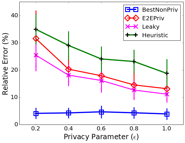
(a)

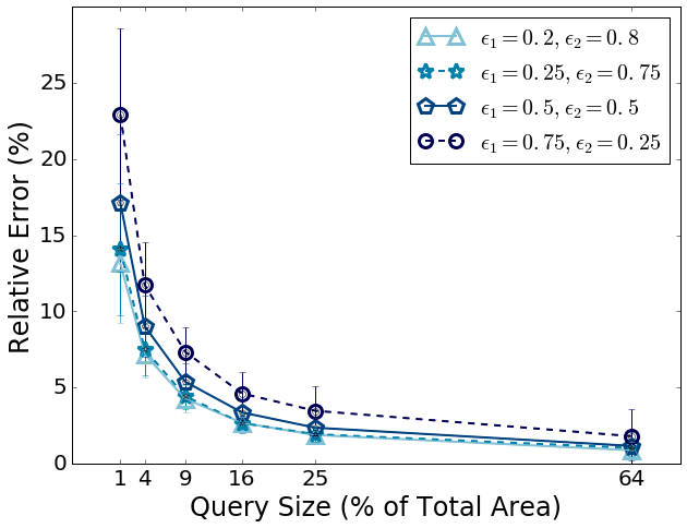
(b)

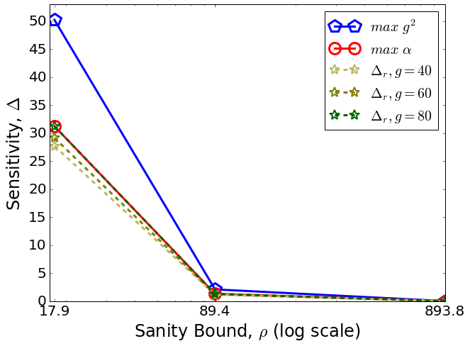
(c)

Figure 11. Effect of (a) varying $\epsilon$ on histogram utility, computed as median relative error; (b) various $\epsilon_{1}$ and $\epsilon_{2}$ on histogram utility, computed as median relative error; (c) sanity bound $\rho$ on sensitivity.

8.7. Effect of Privacy Budget Allocation

Recall that our approach E2EPriv comprises two phases run sequentially, with total privacy budget split between the two phases. In this section, we demonstrate the effect of different budget allocations to each phase and its impact on the released histogram utility via computing the median relative errors for various test $QR$. As shown in Figure 11b, for $\epsilon_{1}\leq 50\%$ the utility of our mechanism remains almost invariant, providing a useful guide for allocating privacy budget.

8.8. Effect of Sanity Bound $\rho$ on Sensitivity

Figure 11c presents the effect of different $\delta$ parameters, and consequently different $\rho=\delta|D|$, on computed sensitivity bounds by the various approaches derived in Section 7: our preferred response-dependent bound (Corollary 7.9), and the two looser response-independent sensitivities (Equations 7 and 8). The results are shown for grid sizes varying through 40, 60 and 80%. As shown, the response-dependent $\Delta_{r}$ does achieve tighter estimates compared to the global alternatives. This difference becomes more significant for reduced sanity bounds, e.g., when $\delta=0.002$ yielding $\rho=17.9$. The $\max\alpha$ alternative sees equivalent values to the maximum grid size approach of response dependent sensitivity.

These results confirm our expectation that using more careful response-dependent sensitivity in the exponential mechanism as applied to E2EPriv tuning’s Phase 1, can lead to better sensitivity estimates which can in-turn lead to superior utility at no cost to privacy.

9. Concluding Remarks

In this paper we propose a first end-to-end differentially-private mechanism for releasing parameter-tuned spatial data structures. Our mechanism E2EPriv leverages a general-purpose concept of tuning via privately-optimising bounds on error: with the bounds on error derived from utility bounds on the data structure release mechanism (in this case existing an application of the Laplace mechanism for releasing histograms); and the private minimisation of these bounds via the exponential mechanism. Key challenges in accomplishing our results included the derivation of error bounds and bounding of these data-dependent error bounds’ sensitivity to perturbation. As a result of our careful analysis, we provide a comprehensive analysis of differential privacy and high-probability utility.

Notably, our bounds on error central to parameter tuning, comprise terms reflecting both aggregation error due to spatial partitioning and perturbation error due to post-tuning differential privacy. Our sensitivity calculations are response-dependent, permitting parameter tuning to achieve superior utility at no cost to privacy over coarse, global sensitivity approaches.

Comprehensive experimental results on datasets of a range of scales, levels of sparsity and uniformity, establish that our principled tuning-and-release mechanism achieves competitive utility while preserving end-to-end differential privacy.

In the literature, parameter tuning has been previously accomplished either non-privately (even tuning differentially-private mechanisms on test data) or by applying fixed parameter guidelines. We establish that neither style of existing approach is sufficient, and that private parameter tuning is achievable, and efficiently implementable.

Appendix A Appendix

A.1. Proof of Theorem 7.5

The theorem’s proof proceeds by cases, based on where $D^{\prime}$’s extra point falls:

1. Outside $QR$, outside overlapping cells (Figure 7a);

2. Outside $QR$, inside overlapping cells (Figure 7b); or

3. Inside $QR$, inside overlapping cells (Figure 7c).

We drop superscripts on $\alpha_{i}$ for readability. Our task is to bound

$$GS(s_{r})=\Delta_{r}s=\max_{\lVert D-D^{\prime}\rVert_{1}\leq 1}\left|s(D,r)-s(D^{\prime},r)\right|$$

$$\leq \left|\frac{1}{\max\{\sum_{i\in\mathcal{C}}d_{i},\rho\}}\left(\left|\sum_{i\in\mathcal{C}}\alpha_{i}c_{i}-\sum_{i\in\mathcal{C}}d_{i}\right|+\lambda\lVert\bm{\alpha}\rVert_{1}\right)-\right.$$

$$\left.\frac{1}{\max\{\sum_{i\in\mathcal{C}}d^{\prime}_{i},\rho^{\prime}\}}\left(\left|\sum_{i\in\mathcal{C}}\alpha_{i}c^{\prime}_{i}-\sum_{i\in\mathcal{C}}d^{\prime}_{i}\right|+\lambda\lVert\bm{\alpha}\rVert_{1}\right)\right|$$

where

$$\rho=\delta\times\left|D\right|\mbox{, }\rho>1$$

$$\rho^{\prime}=\delta\times\left|D^{\prime}\right|=\delta\times(\left|D\right|+1)=\rho+\delta$$

Throughout this proof we are going to have the following expression, which is always positive, so we can drop the absolute:

$$\left|\frac{1}{\max\{\sum_{i\in\mathcal{C}}d_{i},\rho\}}-\frac{1}{\max\{\sum_{i\in\mathcal{C}}d^{\prime}_{i},\rho^{\prime}\}}\right|$$

$$= \frac{1}{\max\{\sum_{i\in\mathcal{C}}d_{i},\rho\}}-\frac{1}{\max\{\sum_{i\in\mathcal{C}}d^{\prime}_{i},\rho^{\prime}\}}$$

Each case as enumerated above, has sub-cases based on the value taken by the denominator.

Case 1. When the extra point is outside $QR$ & outside overlapping cells:

$$\sum_{i\in\mathcal{C}}d^{\prime}_{i}=\sum_{i\in\mathcal{C}}d_{i}\mbox{ \& }c^{\prime}_{i}=c_{i}\Rightarrow$$

$$\left|\sum_{i\in\mathcal{C}}\alpha_{i}c^{\prime}_{i}-\sum_{i\in\mathcal{C}}d^{\prime}_{i}\right|+\lambda\lVert\bm{\alpha}\rVert_{1}=\left|\sum_{i\in\mathcal{C}}\alpha_{i}c_{i}-\sum_{i\in\mathcal{C}}d_{i}\right|+\lambda\lVert\bm{\alpha}\rVert_{1}$$

$$\left|\sum_{i\in\mathcal{C}}\alpha_{i}c_{i}-\sum_{i\in\mathcal{C}}d_{i}\right|+\lambda\lVert\bm{\alpha}\rVert_{1}\leq\left|D\right|+\lambda\lVert\bm{\alpha}\rVert_{1}$$

$$\Delta_{r}s\leq \left(\left|\sum_{i\in\mathcal{C}}\alpha_{i}c_{i}-\sum_{i\in\mathcal{C}}d_{i}\right|+\lambda\lVert\bm{\alpha}\rVert_{1}\right)\cdot\left|\frac{1}{\max\{\sum_{i\in\mathcal{C}}d_{i},\rho\}}-\frac{1}{\max\{\sum_{i\in\mathcal{C}}d^{\prime}_{i},\rho^{\prime}\}}\right|$$

$$\leq \left(\left|D\right|+\lambda\lVert\bm{\alpha}\rVert_{1}\right)\cdot\underbrace{\left(\frac{1}{\rho}-\frac{1}{\rho+\delta}\right)}_{\frac{\delta}{\rho\left(\rho+\delta\right)}=\frac{1}{\left|D\right|\left(\rho+\delta\right)}}\leq\frac{1}{\rho+\delta}+\frac{\lambda\lVert\bm{\alpha}\rVert_{1}}{\left|D\right|\left(\rho+\delta\right)}\enspace.$$

where three possible sub-cases occur:

Case 1.1 $$\boxed{\sum_{i\in\mathcal{C}}d_{i}<\rho<\rho+\delta}$$

$$\max\left\{\sum_{i\in\mathcal{C}}d_{i},\rho\right\}=\rho\mbox{ \& }\max\left\{\sum_{i\in\mathcal{C}}d^{\prime}_{i},\rho^{\prime}\right\}=\rho+\delta$$

$$\Rightarrow\frac{1}{\max\{\sum_{i\in\mathcal{C}}d_{i},\rho\}}-\frac{1}{\max\{\sum_{i\in\mathcal{C}}d^{\prime}_{i},\rho^{\prime}\}}=\frac{1}{\rho}-\frac{1}{\rho+\delta}$$

Case 1.2 $$\boxed{\rho<\rho+\delta<\sum_{i\in\mathcal{C}}d_{i}}$$

$$\max\left\{\sum_{i\in\mathcal{C}}d_{i},\rho\right\}=\sum_{i\in\mathcal{C}}d_{i}\mbox{ \& }\max\left\{\sum_{i\in\mathcal{C}}d^{\prime}_{i},\rho^{\prime}\right\}=\sum_{i\in\mathcal{C}}d_{i}$$

$$\Rightarrow\frac{1}{\max\{\sum_{i\in\mathcal{C}}d_{i},\rho\}}-\frac{1}{\max\{\sum_{i\in\mathcal{C}}d^{\prime}_{i},\rho^{\prime}\}}=\frac{1}{\sum_{i\in\mathcal{C}}d_{i}}-\frac{1}{\sum_{i\in\mathcal{C}}d_{i}}$$

$$= 0$$

Case 1.3 $$\boxed{\rho<\sum_{i\in\mathcal{C}}d_{i}<\rho+\delta}$$

$$\underbrace{\max\left\{\sum_{i\in\mathcal{C}}d_{i},\rho\right\}=\sum_{i\in\mathcal{C}}d_{i}}_{\sum_{i\in\mathcal{C}}d_{i}>\rho\Rightarrow\frac{1}{\sum_{i\in\mathcal{C}}d_{i}}<\frac{1}{\rho}}\mbox{ \& }\underbrace{\max\left\{\sum_{i\in\mathcal{C}}d^{\prime}_{i},\rho^{\prime}\right\}=\rho+\delta}_{\sum_{i\in\mathcal{C}}d_{i}<\rho+\delta\Rightarrow\frac{1}{\sum_{i\in\mathcal{C}}d_{i}}>\frac{1}{\rho+\delta}}$$

$$\Rightarrow\frac{1}{\max\{\sum_{i\in\mathcal{C}}d_{i},\rho\}}-\frac{1}{\max\{\sum_{i\in\mathcal{C}}d^{\prime}_{i},\rho^{\prime}\}}=\frac{1}{\sum_{i\in\mathcal{C}}d_{i}}-\frac{1}{\rho+\delta}$$

$$\Rightarrow\frac{1}{\max\{\sum_{i\in\mathcal{C}}d_{i},\rho\}}-\frac{1}{\max\{\sum_{i\in\mathcal{C}}d^{\prime}_{i},\rho^{\prime}\}}\leq\frac{1}{\rho}-\frac{1}{\rho+\delta}$$

Case 2. When the extra point is outside $QR$ & inside overlapping cells, for some $j$:

$$\sum_{i\in\mathcal{C}}d^{\prime}_{i}=\sum_{i\in\mathcal{C}}d_{i}\mbox{ \& }c^{\prime}_{j}=c_{j}+1\Rightarrow$$

$$\left|\sum_{i\in\mathcal{C}}\alpha_{i}c^{\prime}_{i}-\sum_{i\in\mathcal{C}}d^{\prime}_{i}\right|+\lambda\lVert\bm{\alpha}\rVert_{1}=\left|\sum_{i\in\mathcal{C}}\alpha_{i}c_{i}+\alpha_{j}-\sum_{i\in\mathcal{C}}d_{i}\right|+\lambda\lVert\bm{\alpha}\rVert_{1}$$

$$\Delta_{r}s\leq \left|\frac{1}{\max\{\sum_{i\in\mathcal{C}}d_{i},\rho\}}\left(\left|\sum_{i\in\mathcal{C}}\alpha_{i}c_{i}-\sum_{i\in\mathcal{C}}d_{i}\right|+\lambda\lVert\bm{\alpha}\rVert_{1}\right)-\right.$$

$$\left.\frac{1}{\max\{\sum_{i\in\mathcal{C}}d^{\prime}_{i},\rho^{\prime}\}}\left(\left|\sum_{i\in\mathcal{C}}\alpha_{i}c^{\prime}_{i}-\sum_{i\in\mathcal{C}}d^{\prime}_{i}\right|+\lambda\lVert\bm{\alpha}\rVert_{1}\right)\right|$$

Triangle inequality:

$$\leq \left|\left|\frac{1}{\max\{\sum_{i\in\mathcal{C}}d_{i},\rho\}}\left(\sum_{i\in\mathcal{C}}\alpha_{i}c_{i}-\sum_{i\in\mathcal{C}}d_{i}\right)\right|-\right.$$

$$\left.\left|\frac{1}{\max\{\sum_{i\in\mathcal{C}}d^{\prime}_{i},\rho^{\prime}\}}\left(\sum_{i\in\mathcal{C}}\alpha_{i}c^{\prime}_{i}-\sum_{i\in\mathcal{C}}d^{\prime}_{i}\right)\right|\right|+$$

$$\left|\frac{1}{\max\{\sum_{i\in\mathcal{C}}d_{i},\rho\}}\lambda\lVert\bm{\alpha}\rVert_{1}-\frac{1}{\max\{\sum_{i\in\mathcal{C}}d^{\prime}_{i},\rho^{\prime}\}}\lambda\lVert\bm{\alpha}\rVert_{1}\right|$$

Reverse trianlge inequality:

$$\leq \left|\frac{1}{\max\{\sum_{i\in\mathcal{C}}d_{i},\rho\}}\left(\sum_{i\in\mathcal{C}}\alpha_{i}c_{i}-\sum_{i\in\mathcal{C}}d_{i}\right)-\right.$$

$$\left.\frac{1}{\max\{\sum_{i\in\mathcal{C}}d^{\prime}_{i},\rho^{\prime}\}}\left(\sum_{i\in\mathcal{C}}\alpha_{i}c^{\prime}_{i}-\sum_{i\in\mathcal{C}}d^{\prime}_{i}\right)\right|+$$

$$\lambda\lVert\bm{\alpha}\rVert_{1}\cdot\left|\frac{1}{\max\{\sum_{i\in\mathcal{C}}d_{i},\rho\}}-\frac{1}{\max\{\sum_{i\in\mathcal{C}}d^{\prime}_{i},\rho^{\prime}\}}\right|$$

Rearranging and factoring:

$$\leq \left|\frac{1}{\max\{\sum_{i\in\mathcal{C}}d_{i},\rho\}}\left(\sum_{i\in\mathcal{C}}\alpha_{i}c_{i}-\sum_{i\in\mathcal{C}}d_{i}\right)-\right.$$

$$\left.\frac{1}{\max\{\sum_{i\in\mathcal{C}}d^{\prime}_{i},\rho^{\prime}\}}\left(\left(\sum_{i\in\mathcal{C}}\alpha_{i}c_{i}-\sum_{i\in\mathcal{C}}d_{i}\right)+\alpha_{j}\right)\right|+$$

$$\lambda\lVert\bm{\alpha}\rVert_{1}\cdot\left|\frac{1}{\max\{\sum_{i\in\mathcal{C}}d_{i},\rho\}}-\frac{1}{\max\{\sum_{i\in\mathcal{C}}d^{\prime}_{i},\rho^{\prime}\}}\right|$$

$$\leq \left|\left(\sum_{i\in\mathcal{C}}\alpha_{i}c_{i}-\sum_{i\in\mathcal{C}}d_{i}\right)\left(\frac{1}{\max\{\sum_{i\in\mathcal{C}}d_{i},\rho\}}-\frac{1}{\max\{\sum_{i\in\mathcal{C}}d^{\prime}_{i},\rho^{\prime}\}}\right)-\right.$$

$$\left.\frac{\alpha_{j}}{\max\{\sum_{i\in\mathcal{C}}d^{\prime}_{i},\rho^{\prime}\}}\right|+$$

$$\lambda\lVert\bm{\alpha}\rVert_{1}\cdot\left|\frac{1}{\max\{\sum_{i\in\mathcal{C}}d_{i},\rho\}}-\frac{1}{\max\{\sum_{i\in\mathcal{C}}d^{\prime}_{i},\rho^{\prime}\}}\right|$$

Triangle inequality:

$$\leq \left|\sum_{i\in\mathcal{C}}\alpha_{i}c_{i}-\sum_{i\in\mathcal{C}}d_{i}\right|\cdot\left|\frac{1}{\max\{\sum_{i\in\mathcal{C}}d_{i},\rho\}}-\frac{1}{\max\{\sum_{i\in\mathcal{C}}d^{\prime}_{i},\rho^{\prime}\}}\right|+$$

$$\left|\frac{\alpha_{j}}{\max\{\sum_{i\in\mathcal{C}}d^{\prime}_{i},\rho^{\prime}\}}\right|+$$

$$\lambda\lVert\bm{\alpha}\rVert_{1}\cdot\left|\frac{1}{\max\{\sum_{i\in\mathcal{C}}d_{i},\rho\}}-\frac{1}{\max\{\sum_{i\in\mathcal{C}}d^{\prime}_{i},\rho^{\prime}\}}\right|$$

$$\leq \left(\left|\sum_{i\in\mathcal{C}}\alpha_{i}c_{i}-\sum_{i\in\mathcal{C}}d_{i}\right|+\lambda\lVert\bm{\alpha}\rVert_{1}\right)\cdot$$

$$\left|\frac{1}{\max\{\sum_{i\in\mathcal{C}}d_{i},\rho\}}-\frac{1}{\max\{\sum_{i\in\mathcal{C}}d^{\prime}_{i},\rho^{\prime}\}}\right|+$$

$$\left|\frac{\alpha_{i}}{\max\{\sum_{i\in\mathcal{C}}d^{\prime}_{i},\rho^{\prime}\}}\right|\enspace.$$

$$\leq \left(\left|D\right|+\lambda\lVert\bm{\alpha}\rVert_{1}\right)\cdot\underbrace{\left(\frac{1}{\rho}-\frac{1}{\rho+\delta}\right)}_{\frac{\delta}{\rho\left(\rho+\delta\right)}}+\frac{1}{\rho+\delta}$$

$$\leq \frac{1}{\rho+\delta}+\frac{\lambda\lVert\bm{\alpha}\rVert_{1}}{\left|D\right|\left(\rho+\delta\right)}+\frac{1}{\rho+\delta}\enspace.$$

where cases 1.1, 1.2 and 1.3 apply here as well, and result follows. Case 3. When the extra point is inside both $QR$ & overlapping cells:

$$\sum_{i\in\mathcal{C}}d^{\prime}_{i}=\sum_{i\in\mathcal{C}}d_{i}+1\mbox{ \& }c^{\prime}_{j}=c_{j}+1$$

From case 2 result, we have the following:

$$\Delta_{r}s\leq \Big{|}\frac{1}{\max\{\sum_{i\in\mathcal{C}}d_{i},\rho\}}\left(\sum_{i\in\mathcal{C}}\alpha_{i}c_{i}-\sum_{i\in\mathcal{C}}d_{i}\right)-$$

$$\frac{1}{\max\{\sum_{i\in\mathcal{C}}d^{\prime}_{i},\rho^{\prime}\}}\left(\sum_{i\in\mathcal{C}}\alpha_{i}c^{\prime}_{i}-\sum_{i\in\mathcal{C}}d^{\prime}_{i}\right)\Big{|}+$$

$$\lambda\lVert\bm{\alpha}\rVert_{1}\cdot\left|\frac{1}{\max\{\sum_{i\in\mathcal{C}}d_{i},\rho\}}-\frac{1}{\max\{\sum_{i\in\mathcal{C}}d^{\prime}_{i},\rho^{\prime}\}}\right|$$

$$\leq \left|\frac{1}{\max\{\sum_{i\in\mathcal{C}}d_{i},\rho\}}\left(\sum_{i\in\mathcal{C}}\alpha_{i}c_{i}-\sum_{i\in\mathcal{C}}d_{i}\right)-\right.$$

$$\left.\frac{1}{\max\{\sum_{i\in\mathcal{C}}d^{\prime}_{i},\rho^{\prime}\}}\left(\left(\sum_{i\in\mathcal{C}}\alpha_{i}c_{i}-\sum_{i\in\mathcal{C}}d_{i}\right)+\left(\alpha_{j}-1\right)\right)\right|+$$

$$\lambda\lVert\bm{\alpha}\rVert_{1}\cdot\left|\frac{1}{\max\{\sum_{i\in\mathcal{C}}d_{i},\rho\}}-\frac{1}{\max\{\sum_{i\in\mathcal{C}}d^{\prime}_{i},\rho^{\prime}\}}\right|$$

$$\leq \left(\left|\sum_{i\in\mathcal{C}}\alpha_{i}c_{i}-\sum_{i\in\mathcal{C}}d_{i}\right|+\lambda\lVert\bm{\alpha}\rVert_{1}\right)\cdot$$

$$\left|\frac{1}{\max\{\sum_{i\in\mathcal{C}}d_{i},\rho\}}-\frac{1}{\max\{\sum_{i\in\mathcal{C}}d^{\prime}_{i},\rho^{\prime}\}}\right|+$$

$$\left|\frac{1-\alpha_{j}}{\max\{\sum_{i\in\mathcal{C}}d^{\prime}_{i},\rho^{\prime}\}}\right|$$

$$\leq \left(\left|D\right|+\lambda\lVert\bm{\alpha}\rVert_{1}\right)\cdot\underbrace{\left(\frac{1}{\rho}-\frac{1}{\rho+1}\right)}_{\frac{1}{\rho(\rho+1)}}+\frac{1}{\rho+\delta}$$

$$\leq \frac{1}{\delta(\rho+1)}+\frac{\lambda\lVert\bm{\alpha}\rVert_{1}}{\rho(\rho+1)}+\frac{1}{\rho+\delta}\enspace.$$

where again we have sub cases on the denominator.

Case 3.1 $$\boxed{\sum_{i\in\mathcal{C}}d_{i}<\sum_{i\in\mathcal{C}}d_{i}+1<\rho<\rho+\delta}$$

$$\max\left\{\sum_{i\in\mathcal{C}}d_{i},\rho\right\}=\rho\mbox{ \& }\max\left\{\sum_{i\in\mathcal{C}}d^{\prime}_{i},\rho^{\prime}\right\}=\rho+\delta$$

$$\Rightarrow\frac{1}{\max\{\sum_{i\in\mathcal{C}}d_{i},\rho\}}-\frac{1}{\max\{\sum_{i\in\mathcal{C}}d^{\prime}_{i},\rho^{\prime}\}}=\frac{1}{\rho}-\frac{1}{\rho+\delta}$$

Case 3.2 $$\boxed{\rho<\sum_{i\in\mathcal{C}}d_{i}<\rho+\delta<\sum_{i\in\mathcal{C}}d_{i}+1}$$

$$\underbrace{\max\left\{\sum_{i\in\mathcal{C}}d_{i},\rho\right\}=\sum_{i\in\mathcal{C}}d_{i}}_{\sum_{i\in\mathcal{C}}d_{i}>\rho\Rightarrow\frac{1}{\sum_{i\in\mathcal{C}}d_{i}}<\frac{1}{\rho}}\mbox{ \& }\underbrace{\max\left\{\sum_{i\in\mathcal{C}}d^{\prime}_{i},\rho^{\prime}\right\}=\sum_{i\in\mathcal{C}}d_{i}+1}_{\sum_{i\in\mathcal{C}}d_{i}+1>\rho+\delta\Rightarrow\frac{1}{\sum_{i\in\mathcal{C}}d_{i}+1}<\frac{1}{\rho+\delta}}$$

$$\Rightarrow\frac{1}{\max\{\sum_{i\in\mathcal{C}}d_{i},\rho\}}-\frac{1}{\max\{\sum_{i\in\mathcal{C}}d^{\prime}_{i},\rho^{\prime}\}}=\frac{1}{\sum_{i\in\mathcal{C}}d_{i}}-\frac{1}{\sum_{i\in\mathcal{C}}d_{i}+1}$$

$$\Rightarrow\frac{1}{\max\{\sum_{i\in\mathcal{C}}d_{i},\rho\}}-\frac{1}{\max\{\sum_{i\in\mathcal{C}}d^{\prime}_{i},\rho^{\prime}\}}\leq\frac{1}{\rho}-\frac{1}{\rho+\delta}$$

Case 3.3 $$\boxed{\rho<\sum_{i\in\mathcal{C}}d_{i}<\sum_{i\in\mathcal{C}}d_{i}+1<\rho+\delta}$$

$$\underbrace{\max\left\{\sum_{i\in\mathcal{C}}d_{i},\rho\right\}=\sum_{i\in\mathcal{C}}d_{i}}_{\sum_{i\in\mathcal{C}}d_{i}>\rho\Rightarrow\frac{1}{\sum_{i\in\mathcal{C}}d_{i}}<\frac{1}{\rho}}\mbox{ \& }\underbrace{\max\left\{\sum_{i\in\mathcal{C}}d^{\prime}_{i},\rho^{\prime}\right\}=\rho+\delta}_{\sum_{i\in\mathcal{C}}d_{i}+1<\rho+\delta}$$

$$\Rightarrow\frac{1}{\max\{\sum_{i\in\mathcal{C}}d_{i},\rho\}}-\frac{1}{\max\{\sum_{i\in\mathcal{C}}d^{\prime}_{i},\rho^{\prime}\}}=\frac{1}{\sum_{i\in\mathcal{C}}d_{i}}-\frac{1}{\rho+\delta}$$

$$\Rightarrow\frac{1}{\max\{\sum_{i\in\mathcal{C}}d_{i},\rho\}}-\frac{1}{\max\{\sum_{i\in\mathcal{C}}d^{\prime}_{i},\rho^{\prime}\}}\leq\frac{1}{\rho}-\frac{1}{\rho+\delta}$$

Case 3.4 $$\boxed{\sum_{i\in\mathcal{C}}d_{i}<\rho<\rho+\delta<\sum_{i\in\mathcal{C}}d_{i}+1<\rho+1}$$

$$\underbrace{\max\left\{\sum_{i\in\mathcal{C}}d_{i},\rho\right\}=\rho}_{\begin{subarray}{c}\sum_{i\in\mathcal{C}}d_{i}<\rho\Rightarrow\frac{1}{\sum_{i\in\mathcal{C}}d_{i}}>\frac{1}{\rho}\\ \sum_{i\in\mathcal{C}}d_{i}+1<\rho+1\Rightarrow\frac{1}{\sum_{i\in\mathcal{C}}d_{i}+1}>\frac{1}{\rho+1}\end{subarray}}\mbox{ \& }\underbrace{\max\left\{\sum_{i\in\mathcal{C}}d^{\prime}_{i},\rho^{\prime}\right\}=\sum_{i\in\mathcal{C}}d_{i}+1}_{\begin{subarray}{c}\sum_{i\in\mathcal{C}}d_{i}+1>\rho+\delta\Rightarrow\frac{1}{\sum_{i\in\mathcal{C}}d_{i}+1}<\frac{1}{\rho+\delta}\\ \rho+1>\rho+\delta\Rightarrow\frac{1}{\rho+1}<\frac{1}{\rho+\delta}\end{subarray}}$$

$$\Rightarrow\frac{1}{\max\{\sum_{i\in\mathcal{C}}d_{i},\rho\}}-\frac{1}{\max\{\sum_{i\in\mathcal{C}}d^{\prime}_{i},\rho^{\prime}\}}=\frac{1}{\rho}-\frac{1}{\sum_{i\in\mathcal{C}}d_{i}+1}$$

$$\Rightarrow\frac{1}{\max\{\sum_{i\in\mathcal{C}}d_{i},\rho\}}-\frac{1}{\max\{\sum_{i\in\mathcal{C}}d^{\prime}_{i},\rho^{\prime}\}}\leq\frac{1}{\rho}-\frac{1}{\rho+1}$$

The final upper bound for the response-dependent global sensitivity becomes the bound computed for case 3, as it achieves the maximum over all possible cases.

References

- (1)
- Braz et al. (2007) F. Braz, Salvatore Orlando, Renzo Orsini, Alessandra Raffaetà, Alessandro Roncato, and Claudio Silvestri. 2007. Approximate Aggregations in Trajectory Data Warehouses. In ICDE. 536–545.
- Chaudhuri et al. (2011) Kamalika Chaudhuri, Claire Monteleoni, and Anand D. Sarwate. 2011. Differentially Private Empirical Risk Minimization. JMLR 12 (2011), 1069–1109.
- Chaudhuri and Vinterbo (2013) Kamalika Chaudhuri and Staal A. Vinterbo. 2013. A Stability-based Validation Procedure for Differentially Private Machine Learning. In NIPS. 2652–2660.
- Chawla et al. (2005) Shuchi Chawla, Cynthia Dwork, Frank McSherry, and Kunal Talwar. 2005. On the utility of privacy-preserving histograms. In UAI.
- Chen et al. (2012) Rui Chen, Benjamin C. M. Fung, Bipin C. Desai, and Nériah M. Sossou. 2012. Differentially private transit data publication: a case study on the Montreal transportation system. In KDD. 213–221.
- Cormode et al. (2012) Graham Cormode, Cecilia M. Procopiuc, Divesh Srivastava, Entong Shen, and Ting Yu. 2012. Differentially Private Spatial Decompositions. In ICDE. 20–31.
- Dwork et al. (2006) Cynthia Dwork, Frank McSherry, Kobbi Nissim, and Adam Smith. 2006. Calibrating Noise to Sensitivity in Private Data Analysis. In TCC (LNCS), Vol. 3876. 265–284.
- Dwork and Roth (2014) Cynthia Dwork and Aaron Roth. 2014. The Algorithmic Foundations of Differential Privacy. Foundations and Trends in Theoretical Computer Science 9, 3-4 (2014), 211–407.
- Fanaeepour et al. (2015) Maryam Fanaeepour, Lars Kulik, Egemen Tanin, and Benjamin I. P. Rubinstein. 2015. The CASE histogram: privacy-aware processing of trajectory data using aggregates. GeoInformatica (2015), 1–52.
- Fanaeepour and Rubinstein (2016) Maryam Fanaeepour and Benjamin I. P. Rubinstein. 2016. Beyond Points and Paths: Counting Private Bodies. ICDM (2016), 131–140.
- Garofalakis and Gibbons (2002) Minos N. Garofalakis and Phillip B. Gibbons. 2002. Wavelet synopses with error guarantees. In SIGMOD. 476–487.
- Ghinita (2013) Gabriel Ghinita. 2013. Privacy for Location-based Services. Morgan & Claypool Publishers.
- Hay et al. (2016) Michael Hay, Ashwin Machanavajjhala, Gerome Miklau, Yan Chen, and Dan Zhang. 2016. Principled Evaluation of Differentially Private Algorithms using DPBench. In SIGMOD. 139–154.
- He et al. (2015) Xi He, Graham Cormode, Ashwin Machanavajjhala, Cecilia M. Procopiuc, and Divesh Srivastava. 2015. DPT: Differentially Private Trajectory Synthesis Using Hierarchical Reference Systems. PVLDB 8, 11 (2015), 1154–1165.
- Leonardi et al. (2014) Luca Leonardi, Salvatore Orlando, Alessandra Raffaetà, Alessandro Roncato, Claudio Silvestri, Gennady L. Andrienko, and Natalia V. Andrienko. 2014. A general framework for trajectory data warehousing and visual OLAP. GeoInformatica 18, 2 (2014), 273–312.
- Li et al. (2014) Chao Li, Michael Hay, Gerome Miklau, and Yue Wang. 2014. A Data- and Workload-Aware Query Answering Algorithm for Range Queries Under Differential Privacy. PVLDB 7, 5 (2014), 341–352.
- López et al. (2005) Inés Fernando Vega López, Richard T. Snodgrass, and Bongki Moon. 2005. Spatiotemporal aggregate computation: a survey. IEEE Trans. KDE 17, 2 (2005), 271–286.
- McSherry and Talwar (2007) Frank McSherry and Kunal Talwar. 2007. Mechanism Design via Differential Privacy. In FOCS. 94–103.
- O’Rourke (1998) Joseph O’Rourke. 1998. Computational Geometry in C (2nd ed.). Cambridge University Press, New York, NY, USA.
- Qardaji et al. (2013a) Wahbeh Qardaji, Weining Yang, and Ninghui Li. 2013a. Understanding Hierarchical Methods for Differentially Private Histograms. Proc. VLDB Endow. 6, 14 (2013), 1954–1965.
- Qardaji et al. (2013b) Wahbeh H. Qardaji, Weining Yang, and Ninghui Li. 2013b. Differentially private grids for geospatial data. In ICDE. 757–768.
- Samet (2006) Hanan Samet. 2006. Foundations of multidimensional and metric data structures. Morgan Kaufmann.
- Tao et al. (2004) Yufei Tao, George Kollios, Jeffrey Considine, Feifei Li, and Dimitris Papadias. 2004. Spatio-Temporal Aggregation Using Sketches. In ICDE. 214–225.
- Vitter and Wang (1999) Jeffrey Scott Vitter and Min Wang. 1999. Approximate Computation of Multidimensional Aggregates of Sparse Data Using Wavelets. In SIGMOD. 193–204.
- Zhang et al. (2016) Jun Zhang, Xiaokui Xiao, and Xing Xie. 2016. PrivTree: A Differentially Private Algorithm for Hierarchical Decompositions. In SIGMOD.