One-Pass Error Bounded Trajectory Simplification

Abstract

Nowadays, various sensors are collecting, storing and transmitting tremendous trajectory data, and it is known that raw trajectory data seriously wastes the storage, network band and computing resource. Line simplification ($\mathsf{LS}$) algorithms are an effective approach to attacking this issue by compressing data points in a trajectory to a set of continuous line segments, and are commonly used in practice. However, existing $\mathsf{LS}$ algorithms are not sufficient for the needs of sensors in mobile devices. In this study, we first develop a one-pass error bounded trajectory simplification algorithm ($\mathsf{OPERB}$), which scans each data point in a trajectory once and only once. We then propose an aggressive one-pass error bounded trajectory simplification algorithm ($\mathsf{OPERB}$-$\mathsf{A}$), which allows interpolating new data points into a trajectory under certain conditions. Finally, we experimentally verify that our approaches ($\mathsf{OPERB}$ and $\mathsf{OPERB}$-$\mathsf{A}$) are both efficient and effective, using four real-life trajectory datasets.

1 Introduction

Various mobile devices, such as smart-phones, on-board diagnostics, and wearable smart devices, have been widely using their sensors to collect massive trajectory data of moving objects at a certain sampling rate (e.g., 5 seconds), and transmit it to cloud servers for location based services, trajectory mining and many other applications. It is known that transmitting and storing raw trajectory data consumes too much network bandwidth and storage capacity [15, 11, 12, 18, 4, 10, 3, 2, 20, 22, 21, 13, 19]. Further, we find that the online transmitting of raw trajectories also seriously aggravates several other issues such as out-of-order and duplicate data points in our experiences when implementing an online vehicle-to-cloud data transmission system. Fortunately, these issues can be resolved or greatly alleviated by the trajectory compression techniques [6, 8, 15, 12, 18, 4, 3, 11, 2, 23, 21, 13, 24, 19], among which line simplification based methods are widely used [6, 8, 11, 12, 18, 4, 3, 2, 23], due to their distinct advantages: (a) simple and easy to implement, (b) no need of extra knowledge and suitable for freely moving objects [20], and (c) bounded errors with good compression ratios. Line simplification algorithms belong to lossy compression, and use a set of continuous line segments to represent a compressed trajectory, as shown in Figure 1.

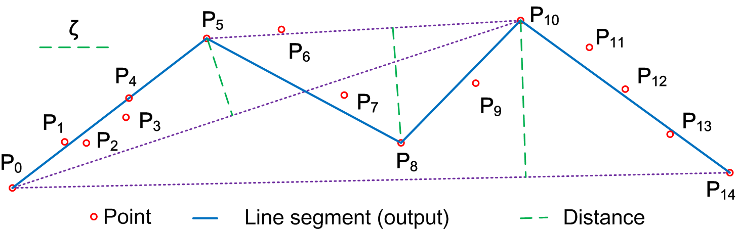
Figure 1: A trajectory $\dddot{\mathcal{T}}[P_{0},\ldots,P_{14}]$ with fifteen points is represented by four continuous line segments (solid blue), compressed by the Douglas–Peucker algorithm [6].

The most notable line simplification ($\mathsf{LS}$) algorithm is the Douglas-Peucker algorithm [6] invented in 1970s, for reducing the number of points required to represent a digitized line or its caricature in the context of computer graphics and image processing. The basic Douglas-Peucker algorithm ($\mathsf{DP}$) is a batch method with a time complexity of $O(n^{2})$, where $n$ is the number of data points in a given trajectory to be compressed. Its batch nature and high time complexity make it not suitable for the online scenarios. Several $\mathsf{LS}$ algorithms have been developed based on $\mathsf{DP}$, e.g., by combining $\mathsf{DP}$ with sliding/open windows [15, 11] for online processing. However, these methods still have a high time and/or space complexity, which significantly hinders their utility in resource-constrained mobile devices [12].

Recently, $\mathsf{BQS}$ [12] has been proposed, using a new distance checking method by picking out at most eight special points from an open window based on a convex hull, e.g., a rectangular bounding box with two bounding lines, so that when a new point is added to a window, it only needs to calculate the distances of the special points to a line, instead of all data points in the window, in many cases. The time complexity of $\mathsf{BQS}$ remains $O(n^{2})$ in the worst case, as $\mathsf{BQS}$ falls back to $\mathsf{DP}$ when the eight special points cannot be used. However, its simplified version, $\mathsf{FBQS}$ directly outputs a line segment, and starts a new window when the eight special points cannot bound all the points considered so far. Indeed, $\mathsf{FBQS}$ has a linear time complexity, and is the fastest $\mathsf{LS}$ based solution for trajectory compression.

An $\mathsf{LS}$ algorithm is one-pass if it processes each point in a trajectory once and only once when compressing the trajectory. Obviously, one-pass algorithms have low time and space complexities, and are more appropriate for online processing. Unfortunately, existing algorithms such as $\mathsf{DP}$, $\mathsf{BQS}$ and $\mathsf{FBQS}$ are not one-pass, as data points in a trajectory are processed multiple times in these algorithms. Indeed, it remains open whether there exist one-pass error bounded $\mathsf{LS}$ based effective trajectory compression algorithms.

Contributions & Roadmap. To this end, we propose two one-pass error bounded $\mathsf{LS}$ based algorithms for compressing trajectories in an efficient and effective way.

(1) We first develop a one-pass error bounded trajectory simplification algorithm ($\mathsf{OPERB}$, Section 4) that runs in $O(n)$ time and $O(1)$ space. $\mathsf{OPERB}$ is based on a novel local distance checking method, and equipped with five optimization techniques to further improve its compression ratio.

(2) We then propose an aggressive one-pass error bounded trajectory simplification algorithm ($\mathsf{OPERB}$-$\mathsf{A}$, Section 5) that remains in $O(n)$ time and $O(1)$ space. $\mathsf{OPERB}$-$\mathsf{A}$ allows interpolating new data points into a trajectory under certain conditions and with practical considerations. The rational lies in that moving objects have sudden track changes while data points may not be sampled due to various reasons.

(3) Using four real-life trajectory datasets ($\mathsf{Taxi}$, $\mathsf{Truck}$, $\mathsf{SerCar}$, $\mathsf{GeoLife}$), we finally conduct an extensive experimental study (Section 6), by comparing our algorithms $\mathsf{OPERB}$ and $\mathsf{OPERB}$-$\mathsf{A}$ with $\mathsf{FBQS}$ (the fastest existing $\mathsf{LS}$ algorithm) and $\mathsf{DP}$ (the best existing $\mathsf{LS}$ algorithm in terms of compression ratio). We find that $\mathsf{OPERB}$ and $\mathsf{OPERB}$-$\mathsf{A}$ are on average $(4.1,4.1,5.4,5.2)$ times faster than $\mathsf{FBQS}$ on ($\mathsf{Taxi}$, $\mathsf{Truck}$, $\mathsf{SerCar}$, $\mathsf{GeoLife}$), respectively. For compression ratios, $\mathsf{OPERB}$ is comparable with $\mathsf{DP}$, and $\mathsf{OPERB}$-$\mathsf{A}$ is better than $\mathsf{DP}$ that is on average ($84.2\%,86.4\%,97.1\%,94.7\%$) of $\mathsf{DP}$ on ($\mathsf{Taxi}$, $\mathsf{Truck}$, $\mathsf{SerCar}$, $\mathsf{GeoLife}$), respectively.

An extended version and some used datasets are at [1].

2 Related Work

Trajectory compression algorithms are normally classified into two categories, namely lossless compression and lossy compression[18]. (1) Lossless compression methods enable exact reconstruction of the original data from the compressed data without information loss. For example, delta compression [19] is a lossless compression technique, which has zero error and a time complexity of $O(n)$, where $n$ is the number of data points in a trajectory. The limitation of lossless compression lies in that its compression ratio is relatively poor [19]. (2) In contrast, lossy compression methods allow errors or derivations, compared with the original trajectories. These techniques typically identify important data points, and remove statistical redundant data points from a trajectory, or replace original data points in a trajectory with other places of interests, such as roads and shops. They focus on good compression ratios with acceptable errors, and a large number of lossy trajectory compression techniques have been developed. In this work we focus on lossy compression of trajectory data,

We next introduce the related work on lossy trajectory compression from two aspects: line simplification based methods and semantics based methods.

Line simplification based methods. Line simplification based methods not only have good compression ratios and deterministic error bounds, but also are easy to implement (see an evaluation report [23])). Hence, they are widely used in practice, even for freely moving objects without the restriction of road networks. And according to the way they process trajectories, they are further divided into batch processing and online processing methods [19].

(1) Batch algorithms require that all trajectory points must be loaded before they start compressing. Batch algorithms can be either top-down or bottom-up. Top-down algorithms recursively divide a trajectory into sub-trajectories until the stopping condition is met[11]. The $\mathsf{DP}$ algorithm [6] is the most classic top-down approach, and [15] improves $\mathsf{DP}$ with the synchronous Euclidean distance, instead of the Euclidean distance. Bottom-up algorithms [11, 3] are the natural complement to top-down ones, which recursively merge adjacent sub-trajectories with the smallest distance, initially $n/2$ sub-trajectories for a trajectory with $n$ points, until the stopping condition is met. Note that the distances of newly generated line segments are recalculated during the process.

(2) Online algorithms do not need to have the entire trajectory ready before they start compressing, and are appropriate for compressing trajectories on sensors of mobile devices. Existing online algorithms [11, 15, 18] usually use a fixed or open window and compress sub-trajectories in the window.

However, these existing online algorithms are not one-pass. In this study, we propose a novel local distance checking method, based on which we develop one-pass online algorithms that are totally different from the window based algorithms. Further, as shown in the experimental study, our approaches are clearly superior to the existing online algorithms, in terms of both efficiency and effectiveness.

Semantics based methods. The trajectories of certain moving objects such as cars and trucks are constrained by road networks. These moving objects typically travel along road networks, instead of the line segment between two points. Trajectory compression methods based on road networks [4, 20, 5, 9, 7, 24] project trajectory points onto roads (also known as Map-Matching). Moreover, [7, 24] mines and uses high frequency patterns of compressed trajectories, instead of roads, to further improve compression effectiveness. Some methods [22, 21] compress trajectories beyond the use of road networks, which further make use of other user specified domain knowledge, such as places of interests along the trajectories [21]. There are also compression algorithms preserving the direction of the trajectory [13, 14].

These approaches are orthogonal to line simplification based methods, and may be combined with each other to further improve the effectiveness of trajectory compression.

3 Preliminaries

In this section, we introduce some basic concepts and existing algorithms for trajectory simplification.

3.1 Basic Notations

Points ($P$). A data point is defined as a triple $P(x,y,t)$, which represents that a moving object is located at longitude $x$ and latitude $y$ at time $t$. Note that data points can be viewed as points in a three-dimension Euclidean space.

Trajectories ($\dddot{\mathcal{T}}$). A trajectory $\dddot{\mathcal{T}}[P_{0},\ldots,P_{n}]$ is a sequence of data points in a monotonically increasing order of their associated time values (i.e., $P_{i}.t<P_{j}.t$ for any $0\leq i<j\leq n$). Intuitively, a trajectory is the path (or track) that a moving object follows through space as a function of time [16].

Directed line segments ($\mathcal{L}$). A directed line segment (or line segment for simplicity) $\mathcal{L}$ is defined as $\vv{P_{s}P_{e}}$, which represents the closed line segment that connects the start point $P_{s}$ and the end point $P_{e}$. Note that here $P_{s}$ or $P_{e}$ may not be a point in a trajectory $\dddot{\mathcal{T}}$, and hence, we also use notation $\mathcal{R}$ instead of $\mathcal{L}$ when both $P_{s}$ and $P_{e}$ belong to $\dddot{\mathcal{T}}$.

We also use $|\mathcal{L}|$ and $\mathcal{L}.\theta\in[0,2\pi)$ to denote the length of a directed line segment $\mathcal{L}$, and its angle with the $x$-axis of the coordinate system $(x,y)$, where $x$ and $y$ are the longitude and latitude, respectively. That is, a directed line segment $\mathcal{L}$ = $\vv{P_{s}P_{e}}$ can be treated as a triple $(P_{s},|\mathcal{L}|,\mathcal{L}.\theta)$.

Piecewise line representation ($\overline{\mathcal{T}}$). A piece-wise line representation of a trajectory $\dddot{\mathcal{T}}[P_{0},\ldots,P_{n}]$ is $\overline{\mathcal{T}}[\mathcal{L}_{0},\ldots,\mathcal{L}_{m}]$ ($0<m\leq n$), a sequence of continuous directed line segments $\mathcal{L}_{i}$ = $\vv{P_{s_{i}}P_{e_{i}}}$ of $\dddot{\mathcal{T}}$ ($i\in[0,m]$) such that $\mathcal{L}_{0}.P_{s_{0}}=P_{0}$, $\mathcal{L}_{m}.P_{e_{m}}=P_{n}$ and $\mathcal{L}_{i}.P_{e_{i}}$ = $\mathcal{L}_{i+1}.P_{s_{i+1}}$ for all $i\in[0,m-1]$. Note that each directed line segment in $\overline{\mathcal{T}}$ essentially represents a continuous sequence of data points in $\dddot{\mathcal{T}}$.

Included angles ($\angle$). Given two directed line segments $\mathcal{L}_{1}$ = $\vv{P_{s}P_{e_{1}}}$ and $\mathcal{L}_{2}$ = $\vv{P_{s}P_{e_{2}}}$ with the same start point $P_{s}$, the included angle from $\mathcal{L}_{1}$ to $\mathcal{L}_{2}$, denoted as $\angle(\mathcal{L}_{1},\mathcal{L}_{2})$, is $\mathcal{L}_{2}.\theta-\mathcal{L}_{1}.\theta$. For convenience, we also represent the included angle $\angle(\mathcal{L}_{1},\mathcal{L}_{2})$ as $\angle{P_{e_{1}}P_{s}P_{e_{2}}}$.

Distances ($d$). Given a point $P_{i}$ and a directed line segment $\mathcal{L}$ = $\vv{P_{s}P_{e}}$, the distance of $P_{i}$ to $\mathcal{L}$, denoted as $d(P_{i},\mathcal{L})$, is the Euclidean distance from $P_{i}$ to the line $\overline{P_{s}P_{e}}$, commonly adopted by most existing $\mathsf{LS}$ methods, e.g., [6, 8, 11, 3, 12].

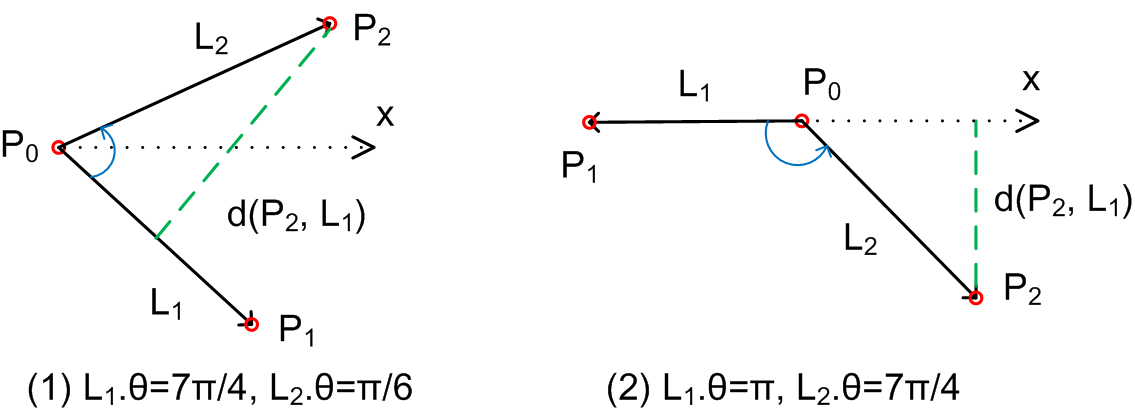
Figure 2: Example included angles and distances.

Example 3.1.

(1) In Figure 1, the four continuous directed line segments $\vv{P_{0}P_{5}}$, $\vv{P_{5}P_{8}}$, $\vv{P_{8}P_{10}}$, $\vv{P_{10}P_{14}}$ form a piecewise line representation of trajectory $\dddot{\mathcal{T}}[P_{0}$, $\ldots,P_{14}]$.

(2) Figure 2 shows two different cases of included angles. In each case, there are two directed line segments $\mathcal{L}_{1}=\vv{P_{0}P_{1}}$ and $\mathcal{L}_{2}=\vv{P_{0}P_{2}}$ with the same start point $P_{0}$. The included angle $\angle(\mathcal{L}_{1},\mathcal{L}_{2})$ from $\mathcal{L}_{1}$ to $\mathcal{L}_{2}$ lies in $(-2\pi,2\pi)$, and is $\frac{-19\pi}{12}$ and $\frac{3\pi}{4}$ in Figures 2(1)&(2), respectively.

(3) The distance $d(P_{2},\mathcal{L}_{1})$ is illustrated in Figures 2 as dotted green line segments.

3.2 Line Simplification Algorithms

Line simplification ($\mathsf{LS}$) algorithms are a type of important and widely adopted trajectory compression methods, and we next briefly introduce these algorithms.

Basic Douglas-Peucker algorithm. We first introduce the Basic Douglas-Peucker ($\mathsf{DP}$) algorithm [6] shown in Figure 3, the foundation of many subsequent $\mathsf{LS}$ algorithms.

Given a trajectory $\dddot{\mathcal{T}}[P_{0},\ldots,P_{n}]$ and an error bound $\zeta$, algorithm $\mathsf{DP}$ uses the first point $P_{0}$ and the last point $P_{n}$ of $\dddot{\mathcal{T}}$ as the start point $P_{s}$ and the end point $P_{e}$ of the first line segment $\mathcal{L}(P_{0},P_{n})$, then it calculates the distance $d(P_{i},{\mathcal{L}})$ for each point $P_{i}$ ($i\in[0,n]$) (lines 1–2). If $d(P_{k},{\mathcal{L}})$ = $\max\{d(P_{0},{\mathcal{L}}),\ldots,d(P_{n},{\mathcal{L}})\}\leq\zeta$, then it returns $\{\mathcal{L}(P_{0},P_{n})\}$ (lines 3–5). Otherwise, it divides $\dddot{\mathcal{T}}$ into two sub-trajectories $\dddot{\mathcal{T}}$$[P_{0},\ldots,P_{k}]$ and $\dddot{\mathcal{T}}$$[P_{k},\ldots,P_{n}]$, and recursively compresses these sub-trajectories until the entire trajectory has been considered (lines 6–7).

The $\mathsf{DP}$ algorithm is clearly a batch algorithm, as the entire trajectory is needed at the beginning [15], and its time complexity is $O(n^{2})$. Moreover, [8] developed an improved method with a time complexity of $O(n\log n)$.

 

	Algorithm ${\mathsf{DP}}(\dddot{\mathcal{T}}[P_{0},\ldots,P_{n}],\zeta)$
1.	for each point $P_{i}$ ($i\in[0,n]$) in $\dddot{\mathcal{T}}[P_{0},\ldots,P_{n}]$ do
2.	compute $d(P_{i},{\mathcal{L}})$ between $P_{i}$ and ${\mathcal{L}}(P_{0},P_{n})$;
3.	let $d(P_{k},{\mathcal{L}})$ := $\max\{d(P_{0},{\mathcal{L}}),\ldots,d(P_{n},{\mathcal{L}})\}$;
4.	if $d(P_{k},{\mathcal{L}})\leq\zeta$ then
5.	return $\{\mathcal{L}(P_{0},P_{n})\}$.
6.	else
7.	return ${\mathsf{DP}}($$\dddot{\mathcal{T}}$$[P_{0},\ldots,P_{k}],\zeta)\cup{\mathsf{DP}}($$\dddot{\mathcal{T}}$$[P_{k},\ldots,P_{n}],\zeta)$.

 

Figure 3: Basic Douglas-Peucker algorithm

Example 3.2.

Consider the trajectory $\dddot{\mathcal{T}}[P_{0},\ldots,P_{14}]$ shown in Figure 1. Algorithm ${\mathsf{DP}}$ firstly creates $\vv{P_{0}P_{14}}$, then it calculates the distance of each point in $\{P_{0},\ldots,P_{14}\}$ to $\vv{P_{0}P_{14}}$. It finds that $P_{10}$ has the maximum distance to $\vv{P_{0}P_{14}}$, which is greater than $\zeta$. Then it goes to compress sub-trajectories $[P_{0},\ldots,P_{10}]$ and $[P_{10},\ldots,P_{14}]$, separately. Similarly, sub-trajectory $[P_{0},\ldots,P_{10}]$ is split to $[P_{0}$, $\ldots$, $P_{5}]$ and $[P_{5}$, $\ldots$, $P_{10}]$, and $[P_{5}$, $\ldots$, $P_{10}]$ is split to $[P_{5},\ldots,P_{8}]$ and $[P_{8}$, $P_{9}$, $P_{10}]$. Finally, algorithm ${\mathsf{DP}}$ outputs four continuous directed line segments $\{\vv{P_{0}P_{5}}$, $\vv{P_{5}P_{8}}$, $\vv{P_{8}P_{10}}$, $\vv{P_{10}P_{14}}\}$, i.e., a piece-wise line representation of trajectory $\dddot{\mathcal{T}}[P_{0},\ldots,P_{14}]$

Online algorithms. We next introduce two classes of $\mathsf{DP}$ based online algorithms that make use of sliding windows to speed up the compressing efficiency [15, 11, 12].

Given a trajectory $\dddot{\mathcal{T}}[P_{0},\ldots,P_{n}]$ and an error bound $\zeta$, algorithm $\mathsf{OPW}$ [15] maintains a window $W[P_{s},\ldots,P_{k}]$, where $P_{s}$ and $P_{k}$ are the start and end points, respectively. Initially, $P_{s}$ = $P_{0}$ and $P_{k}$ = $P_{1}$, and the window $W$ is gradually expanded by adding new points one by one. $\mathsf{OPW}$ tries to compress all points in $W[P_{s},\ldots,P_{k}]$ to a single line segment $\mathcal{L}(P_{s},P_{k})$. If the distances $d(P_{i},{\mathcal{L}})\leq\zeta$ for all points $P_{i}$ ($i\in[s,k]$), it simply expands $W$ to $[P_{s},\ldots,P_{k},P_{k+1}]$ $(k+1\leq n)$ by adding a new point $P_{k+1}$. Otherwise, it produces a new line segment $\mathcal{L}(P_{s},P_{k-1})$, and replaces $W$ with a new window $[P_{k-1},\ldots,P_{k+1}]$. The above process repeats until all points in $\dddot{\mathcal{T}}$ have been considered. Algorithm $\mathsf{OPW}$ is not efficient enough for compressing long trajectories as it remains in $O(n^{2})$ time, the same as the $\mathsf{DP}$ algorithm.

$\mathsf{BQS}$ [12] reduces the compression time by introducing a convex hull that bounds a certain number of points. For a buffered sub trajectory $[P_{s},\ldots,P_{k}]$, it splits the space into four quadrants. For each quadrant, a rectangular bounding box is firstly created using the least and highest $x$ values and the least and highest $y$ values among points $P_{s},\ldots,P_{k}$. Then another two bounding lines connecting points $P_{s}$ and $P_{h}$ and points $P_{s}$ and $P_{l}$ are created such that lines $\overline{P_{s}P_{h}}$ and $\overline{P_{s}P_{l}}$ have the largest and smallest angles with the $x$-axis, respectively. Here $P_{h},P_{l}\in\{P_{s},\ldots,P_{k}\}$. The bounding box and the two lines together form a convex hull. $\mathsf{BQS}$ picks out at most eight significant points in a quadrant. In many cases, (1) it only calculates the distances of the significant points to line $\overline{P_{s}P_{k}}$; otherwise, (2) it needs to compute all distances $d(P_{i},{\mathcal{L}(P_{s},P_{k})})$ ($i\in[s,k]$) as $\mathsf{DP}$. $\mathsf{BQS}$ remains in $O(n^{2})$ time. However, its simplified version $\mathsf{FBQS}$ essentially avoids case (2) to achieve an $O(n)$ time complexity.

Example 3.3.

In Figure 4, the bounding box $c_{1}c_{2}c_{3}c_{4}$ and the two lines $\overline{P_{s}P_{h}}=\overline{P_{0}P_{1}}$ and $\overline{P_{s}P_{l}}=\overline{P_{0}P_{2}}$ form a convex hull $u_{1}u_{2}c_{2}l_{2}l_{1}c_{4}$. $\mathsf{BQS}$ computes the distances of $u_{1},u_{2},c_{2},l_{2},l_{1}$ and $c_{4}$ to line $\overline{P_{0}P_{6}}$ when $k=6$ or to line $\overline{P_{0}P_{7}}$ when $k=7$.

When $k=6$, all these distances to $\overline{P_{0}P_{6}}$ are less than $\zeta$, hence $\mathsf{BQS}$ goes on to the next point (case 1); When $k=7$, the max and min distances to $\overline{P_{0}P_{7}}$ are larger and less than $\zeta$, respectively, and $\mathsf{BQS}$ needs to compress sub-trajectory $[P_{0},\ldots,P_{7}]$ along the same line as $\mathsf{DP}$ (case 2).

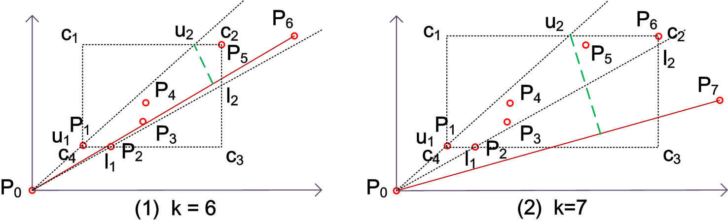
Figure 4: Examples for algorithm $\mathsf{BQS}$.

Error bounded algorithms. Given a trajectory $\dddot{\mathcal{T}}$ and its compression algorithm $\mathcal{A}$ that produces another trajectory $\dddot{\mathcal{T^{\prime}}}$, we say that algorithm $\mathcal{A}$ is error bounded by $\zeta$ if for each point $P$ in $\dddot{\mathcal{T}}$, there exists a point $P_{j}$ in $\dddot{\mathcal{T^{\prime}}}$ with $d(P,\mathcal{L}(P_{j},P_{j+1}))\leq\zeta$. Note that all the above $\mathsf{LS}$ algorithms are error bounded by $\zeta$, a parameter typically set by experts based on the need and analysis of applications.

4 One-Pass Simplification

In this section, we first develop a local distance checking approach that is the key for one-pass trajectory simplification algorithms. We then present a One-Pass ERror Bounded trajectory simplification algorithm, referred to as $\mathsf{OPERB}$. Finally, we propose five optimization techniques.

4.1 Local Distance Checking

Existing trajectory simplification algorithms (e.g., $\mathsf{DP}$ [6] and online algorithms [15, 11, 12]) essentially employ a global distance checking approach to assuring error bounds, although online algorithms restrict the checking within a window. That is to say, whenever a new directed line segment $\mathcal{R}_{i}$ = $\vv{P_{s}P_{s+i}}$ $(i\in[1,k])$ is formed for a sub-trajectory $\dddot{\mathcal{T}_{s}}[P_{s},\ldots,P_{s+k}]$, these algorithms always check its distances to all or a subset of data points $\{P_{s},\ldots,P_{s+i}\}$ to $\mathcal{R}_{i}$, and, therefore, a data point is checked multiple times, depending on its order in the trajectory and the number of directed line segments formed. Hence, an appropriate local distance checking approach is needed in the first place for designing one-pass trajectory simplification algorithms.

Consider an error bound $\zeta$ and a sub-trajectory $\dddot{\mathcal{T}_{s}}[P_{s},$ $\ldots,P_{s+k}]$. To achieve the local distance checking, $\mathsf{OPERB}$ first dynamically maintains a directed line segment $\mathcal{L}_{i}$ ($i\in[1,k]$), whose start point is fixed with $P_{s}$ and its end point is identified (may not in $\{P_{s},\ldots,P_{s+i}\}$) to fit all the previously processed points $\{P_{s},\ldots,P_{s+i}\}$. The directed line segment $\mathcal{L}_{i}$ is built by a function named fitting function $\mathbb{F}$, such that when a new point $P_{s+i+1}$ is considered, only its distance to the directed line segment $\mathcal{L}_{i}$ is checked, instead of checking the distances of all or a subset of data points of $\{P_{s},\ldots,P_{s+i}\}$ to $\mathcal{R}_{i+1}$ = $\vv{P_{s}P_{s+i+1}}$ as the global distance checking does. In this way, a data point is checked only once during the entire process of trajectory simplification.

We next present the details of our fitting function $\mathbb{F}$ that is designed for local distance checking.

Fitting function $\mathbb{F}$. Given an error bound $\zeta$ and a sub-trajectory $\dddot{\mathcal{T}_{s}}[P_{s},\ldots,P_{s+k}]$, $\mathbb{F}$ is as follows.

$$\left\{\begin{aligned} &\left[\begin{aligned} &\mathcal{L}_{i}=\mathcal{L}_{i-1}\\ \end{aligned}\right]\hskip 48.4373pt\leavevmode\nobreak\ when\leavevmode\nobreak\ (|\mathcal{R}_{i}|-|\mathcal{L}_{i-1}|)\leq\frac{\zeta}{4}\hskip 56.18727pt(1)\\ &\left[\begin{aligned} &|\mathcal{L}_{i}|=j*{\zeta}/{2}\\ &\mathcal{L}_{i}.\theta=\mathcal{R}_{i}.\theta\\ \end{aligned}\right]\hskip 32.93736pt\leavevmode\nobreak\ when\leavevmode\nobreak\ |\mathcal{R}_{i}|>\frac{\zeta}{4}\leavevmode\nobreak\ \mbox{\bf and}\ \leavevmode\nobreak\ |\mathcal{L}_{i-1}|=0\hskip 30.99988pt(2)\leavevmode\nobreak\ \\ &\left[\begin{aligned} &|\mathcal{L}_{i}|=j*{\zeta}/{2}\\ &\mathcal{L}_{i}.\theta=\mathcal{L}_{i-1}.\theta+f(\mathcal{R}_{i},\mathcal{L}_{i-1})*\arcsin(\frac{d(P_{s+i},\mathcal{L}_{i-1})}{j*\zeta/2})/j\\ \end{aligned}\right]\leavevmode\nobreak\ else\hskip 3.87498pt(3)\\ \end{aligned}\right.$$

where (a) $1\leq i\leq k+1$; (b) $\mathcal{R}_{i-1}$ = $\vv{P_{s}P_{s+i-1}}$, is the directed line segment whose end point $P_{s+i-1}$ is in $\dddot{\mathcal{T}_{s}}[P_{s},\ldots,P_{s+k}]$; (c) $\mathcal{L}_{i}$ is the directed line segment built by fitting function $\mathbb{F}$ to fit sub-trajectory $\dddot{\mathcal{T}_{s}}[P_{s},\ldots,P_{s+i}]$ and $\mathcal{L}_{0}$ = $\mathcal{R}_{0}$; (d) $j=\lceil(|\mathcal{R}_{i}|*2/\zeta-0.5)\rceil$; (e) $f()$ is a sign function such that $f(\mathcal{R}_{i},\mathcal{L}_{i-1})$ = $1$ if the included angle $\angle(\mathcal{R}_{i-1},\mathcal{R}_{i})$ = $(\mathcal{R}_{i}.\theta-\mathcal{L}_{i-1}.\theta)$ falls in the range of $(-2\pi,-\frac{3\pi}{2}]$, $[-\pi,-\frac{\pi}{2}]$, $[0,\frac{\pi}{2}]$ and $[\pi,\frac{3\pi}{2})$, and $f(\mathcal{R}_{i},\mathcal{L}_{i-1})$ = $-1$, otherwise; (f) $\zeta/2$ is a step length to control the increment of $|\mathcal{L}|$.

Given any sub-trajectory $\dddot{\mathcal{T}_{s}}[P_{s}$, $\ldots$, $P_{s+k}]$ and any error bound $\zeta$, the expression $j=\lceil(|\mathcal{R}_{i}|*2/\zeta-0.5)\rceil$ in the fitting function $\mathbb{F}$ essentially partitions the space into zones around the center point $P_{s}$ such that for each $j\geq 0$, zone $Z_{j}$ = $\{P_{j}\ |\ j*\zeta/2-\zeta/4<|\vv{P_{s}P_{j}}|\leq j*\zeta/2+\zeta/4\}$, i.e., the radii of $Z_{0},Z_{1},Z_{2}$ and $Z_{3}$ to $P_{s}$ are in the ranges of $(-\frac{1}{4}\zeta,\frac{1}{4}\zeta]$, $(\frac{1}{4}\zeta,\frac{3}{4}\zeta]$, $(\frac{3}{4}\zeta,\frac{5}{4}\zeta]$ and $(\frac{5}{4}\zeta,\frac{7}{4}\zeta]$, respectively, and all ranges have a fixed size $\zeta/2$ as shown in Figure 5. Moreover, the angle of the directed line segment $\mathcal{L}_{i}$ is adjusted from $\mathcal{L}_{i-1}$ to make it closer to $P_{s+i}$ than $\mathcal{L}_{i-1}$, i.e., $d(P_{s+i},\mathcal{L}_{i})\leq d(P_{s+i},\mathcal{L}_{i-1})$ for any $i\in(s,s+k]$, and the angle from $\mathcal{L}_{1}$ to $\mathcal{L}_{k}$ is bounded by a constant (Lemma 4.2).

The fitting function $\mathbb{F}$ also creates a virtual stepwise sub-trajectory $\dddot{\mathcal{T}_{v}}[V_{s}$, $\ldots$, $V_{s+l}]$ such that $V_{s}=P_{s}$, $|\vv{V_{s}V_{s+j}}|$ = $\zeta/2*j$ $(j\in[0,l],0<l\leq k)$. For each point $P_{s+i}$ in the sub trajectory, it is mapped to a virtual point $V_{s+j}$ in $\dddot{\mathcal{T}_{v}}$ locating in zone $Z_{j}$. Observe that (a) it is possible that $(|\mathcal{R}_{i}|-|\mathcal{L}_{i-1}|)\leq 0$, (b) the fitting function $\mathbb{F}$ forms a directed line segment $\mathcal{L}_{i}$, which is closer to $\mathcal{R}_{i}$ than $\mathcal{L}_{i-1}$, and partitions the points in the sub-trajectory $\dddot{\mathcal{T}}$ into two classes:

(1) Active points. Points $P_{s}$ and $P_{s+i}$ such that $|\mathcal{R}_{i}|-|\mathcal{L}_{i-1}|$ $>$ $\zeta/4$ are referred to as active points. An active point $P_{s+i}$ is mapped to the virtual point in zone $Z_{j}$ with $j=\lceil(|\mathcal{R}_{i}|*2/\zeta-0.5)\rceil$, and each zone has at most one active point.

(2) Inactive points. Points $P_{s+i}$ such that $|\mathcal{R}_{i}|-|\mathcal{L}_{i-1}|\leq\zeta/4$ are referred to as inactivated points. For an inactive point $P_{s+i}$, it is mapped to zone $Z_{j}$ with $j=|\mathcal{L}_{i-1}|*2/\zeta$. There may exist none or multiple inactive points in a zone.

We next explain the fitting function $\mathbb{F}$ with an example.

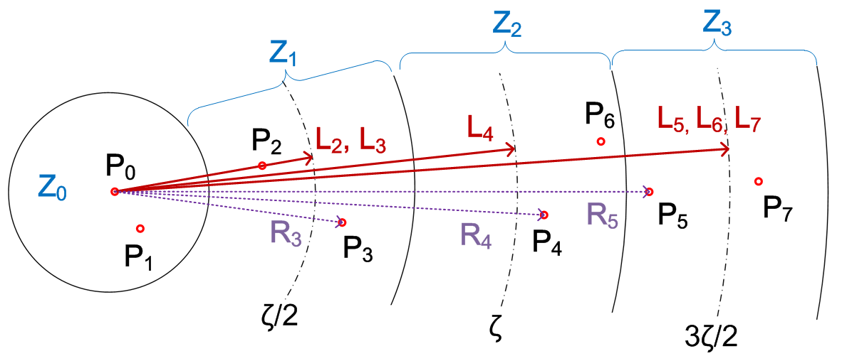
Figure 5: An example of the fitting function

Example 4.4.

Consider the sub-trajectory $[P_{0},\ldots,P_{7}]$ in Figure 5 whose eight points fall in zones $Z_{0},Z_{1},Z_{2},Z_{3}$.

(1) Point $P_{0}$ is the start point and the first active point, and $\mathcal{L}_{0}=\mathcal{R}_{0}=\vv{P_{0}P_{0}}$.

(2) Point $P_{1}$ is inactive in zone $Z_{0}$, as $|\mathcal{R}_{1}|$ = $|\vv{P_{0}P_{1}}|$ $<$ $\frac{\zeta}{4}$ and $(|\mathcal{R}_{1}|-|\mathcal{L}_{0}|)\leq\frac{\zeta}{4}$. Hence, $\mathcal{L}_{1}=\mathcal{L}_{0}$ (case (1)).

(3) Point $P_{2}$ is active in $Z_{1}$, as $|\mathcal{R}_{2}|>\frac{\zeta}{4}$ and $|\mathcal{L}_{1}|=0$ . Hence, $|\mathcal{L}_{2}|=\frac{\zeta}{2}$ and $\mathcal{L}_{2}.\theta=\mathcal{R}_{2}.\theta$ (case 2).

(4) Point $P_{3}$ is inactive in $Z_{1}$, as $(|\mathcal{R}_{3}|-|\mathcal{L}_{2}|)\leq\frac{\zeta}{4}$. Hence, $\mathcal{L}_{3}=\mathcal{L}_{2}$ (case 1).

(5) Point $P_{4}$ is active in $Z_{2}$, as $|\mathcal{R}_{4}|-|\mathcal{L}_{3}|)>\frac{\zeta}{4}$ and $|\mathcal{L}_{3}|\neq 0$. Hence, $|\mathcal{L}_{4}|=2*\frac{\zeta}{2}=\zeta$ and the angle of $\mathcal{L}_{4}$ is also calculated accordingly (case 3).

(6) Similarly, point $P_{5}$ is active in $Z_{3}$ (case 3), and points $P_{6}$ and $P_{7}$ are inactive (case 1). Here $P_{6}$ is mapped to $Z_{3}$ as $|\mathcal{L}_{5}|=\frac{3}{2}\zeta$ though it is physically located in zone $Z_{2}$.

4.2 Analyses of the Fitting Function

We next give an analysis of the fitting function $\mathbb{F}$. First, by the definition of $\mathbb{F}$, it is easy to have the following.

Proposition 4.5: Given any sub-trajectory $\dddot{\mathcal{T}_{s}}[P_{s},\ldots,P_{s+k}]$ and error bound $\zeta$, the directed line segment $\mathcal{L}_{i}$ $(i\in[1,k])$ can be computed by the fitting function $\mathbb{F}$ in $O(1)$ time. $\Box$

The fitting function $\mathbb{F}$ also enables a local distance checking method, as shown below.

Theorem 4.6: Given any sub-trajectory $\dddot{\mathcal{T}_{s}}[P_{s},\ldots,P_{s+k}]$ with $k\leq 4\times 10^{5}$ and error bound $\zeta$, then $d(P_{s+i},{\vv{P_{s}P_{s+k}})}\leq\zeta$ for each $i\in[0,k]$ if $P_{s+k}$ is an active point and $d(P_{s+i},\mathcal{L}_{i-1})\leq\zeta/2$ for each $i\in[1,k]$. $\Box$

To prove Theorem 4.2, we first introduce a special class of trajectories, based on which we show that Theorem 4.2 holds.

Stepwise trajectories. We say that a trajectory $\dddot{\mathcal{T}}[P_{s}$, $\ldots$, $P_{s+k}]$ is stepwise w.r.t. $\zeta/2$ if and only if $|\mathcal{R}_{i}|=i*\zeta/2$ for each directed line segment $\mathcal{R}_{i}$ = $\vv{P_{s}P_{s+i}}$ ($i\in[0,k]$).

Observe that $|\mathcal{R}_{i}|$ $-$ $|\mathcal{R}_{i-1}|$ = $\zeta/2$ and $\lceil|\mathcal{R}_{i}|*2/\zeta-0.5\rceil=i$ ($i\in[1,k]$). Hence, for stepwise sub-trajectories $\dddot{\mathcal{T}}[P_{s}$, $\ldots$, $P_{s+k}]$, the fitting function can be simplified as $\mathbb{F}^{\prime}$ below.

$$\left\{\begin{aligned} &\left[\begin{aligned} &\mathcal{L}_{1}={\zeta}/{2}\\ &\mathcal{L}_{1}.\theta=\mathcal{R}_{1}.\theta\\ \end{aligned}\right]\hskip 180.18678pt\leavevmode\nobreak\ i=1\hskip 3.87498pt(1)\\ &\left[\begin{aligned} &|\mathcal{L}_{i}|=i*{\zeta}/{2}\\ &\mathcal{L}_{i}.\theta=\mathcal{L}_{i-1}.\theta+f(\mathcal{R}_{i},\mathcal{L}_{i-1})*\arcsin(\frac{d(P_{s+i},\mathcal{L}_{i-1})}{i*\zeta/2})/i\\ \end{aligned}\right]\hskip 1.93748pti\geq 2\hskip 3.87498pt(2)\leavevmode\nobreak\ \\ \end{aligned}\right.$$

Stepwise trajectories have the following properties.

Lemma 4.7: Given any sub-trajectory $\dddot{\mathcal{T}_{s}}[P_{s},\ldots,P_{s+k}]$ and error bound $\zeta$, if $d(P_{s+i},\mathcal{L}_{i-1})\leq\frac{\zeta}{2}$ for each $i$ $\in[2,k]$, then the angle change between $\mathcal{L}_{1}$ and $\mathcal{L}_{k}$ is bounded by $\Delta\theta$ = $\lim\limits_{k\to\infty}{\sum_{i=2}^{k}\frac{1}{i}*{\arcsin(\frac{1}{i})}}<0.8123$ (or $46.54^{o}$). $\Box$

Proof 4.8.

By the revised fitting function $\mathbb{F^{\prime}}$ for a stepwise sub-trajectory and $d(P_{s+i},\mathcal{L}_{i-1})\leq\frac{\zeta}{2}$ for all $i$ $\in[2,k]$, we have $\Delta\theta$ $\leq{\sum_{i=2}^{k}\frac{1}{i}*{\arcsin(\frac{1}{i})}}$, which is monotonically increasing with the increment of $k$. As $x\leq\arcsin(x)\leq{x}/{\sqrt{1-x^{2}}}$ ($0\leq x<1$), we also have $\frac{1}{i}\leq\arcsin\frac{1}{i}\leq$ ${1}/{\sqrt{i^{2}-1}}$ ($i\geq 2$).

Hence, we have $\Delta\theta\leq\lim\limits_{k\to\infty}{\sum_{i=2}^{k}(\frac{1}{i}*\frac{1}{\sqrt{i^{2}-1}})}$ $<{\int_{2}^{\infty}(\frac{1}{x}*\frac{1}{\sqrt{x^{2}-1}})}dx+\frac{1}{2}*\frac{1}{\sqrt{2^{2}-1}}=\frac{\pi}{6}+\frac{1}{2\sqrt{3}}\approx 0.8123$.

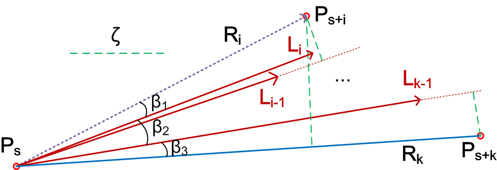
Figure 6: Example for the proof of Lemma 6

Lemma 4.9: Given any sub-trajectory $\dddot{\mathcal{T}_{s}}[P_{s},\ldots,P_{s+k}]$ with $k\leq 4\times 10^{5}$ and error bound $\zeta$, then $d(P_{s+i},{\vv{P_{s}P_{s+k}})}\leq\zeta$ for each $i\in[0,k]$ if $d(P_{s+i},\mathcal{L}_{i-1})\leq\frac{\zeta}{2}$ for each $i\in[1,k]$. $\Box$

Proof 4.10.

Consider the four directed line segments $\mathcal{R}_{i}=\vv{P_{s}P_{s+i}}$, $\mathcal{R}_{k}=\vv{P_{s}P_{s+k}}$, $\mathcal{L}_{i-1}$ and $\mathcal{L}_{k-1}$ shown in Figure 6. Further, let $\beta_{1}$ = $\mathcal{R}_{i}.\theta-\mathcal{L}_{i-1}.\theta$, $\beta_{2}$ = $\mathcal{L}_{k-1}.\theta-\mathcal{L}_{i}.\theta$, $\beta_{3}$ = $\mathcal{R}_{k}.\theta-\mathcal{L}_{k-1}.\theta$. We then adjust the included angles $\beta_{1}$ as follows: (a) if $\frac{\pi}{2}<|\beta_{1}|\leq\pi$, $\beta_{1}$ = $\pi$ - $\beta_{1}$, (b) if $\pi<|\beta_{1}|\leq\frac{3}{2}\pi$, $\beta_{1}$ = $\beta_{1}$ - $\pi$, (c) if $\frac{3}{2}\pi<|\beta_{1}|\leq{2}\pi$, $\beta_{1}$ = $2\pi$ - $\beta_{1}$, and (d) $\beta_{1}$ = $|\beta_{1}|$, otherwise. The included angle $\beta_{3}$ is adjusted along the same line as $\beta_{1}$, and $\beta_{2}$ is bounded by Lemma 4.2.

Observe that $d(P_{s+i},\mathcal{R}_{k})\leq i*\frac{\zeta}{2}*\sin(|\beta_{1}|+|\beta_{2}|+|\beta_{3}|)$ $\leq$ $i*\frac{\zeta}{2}*\sin(\arcsin\frac{1}{i}+\sum_{j=i+1}^{k-1}{(\frac{1}{j}*\arcsin\frac{1}{j})}+\arcsin\frac{1}{k})$. For any $k\leq 4\times 10^{5}$, $i*\sin(|\beta_{1}|+|\beta_{2}|+|\beta_{3}|)<2$, and, hence, we have $d(P_{s+i},\mathcal{R}_{k})<\frac{\zeta}{2}*2=\zeta$.

By mapping inactive and active points of a trajectory to virtual points of a trajectory stepwise w.r.t. ${\zeta}/2$, one can readily prove Theorem 4.2 along the lines as Lemma 6.

Remarks. (1) Our fitting function achieves local distance checking, as indicated by Proposition 4.2 and Theorem 4.2; (2) For a sub-trajectory $\dddot{\mathcal{T}_{s}}[P_{s},\ldots,P_{s+k-1}]$ represented by a single directed line segment, we restrict $k\leq 4*10^{5}$, which suffices for the need of trajectory simplification in practice.

4.3 Algorithm OPERB

We are now ready to present our one-pass error bounded algorithm, which makes use of the local distance checking method based on the fitting function $\mathbb{F}$.

The main result of this section is as follows.

Theorem 4.11: Given any trajectory $\dddot{\mathcal{T}}[P_{0},\ldots,P_{n}]$ and error bound $\zeta$, there exists a one-pass trajectory simplification algorithm that is error bounded by $\zeta$. $\Box$

We prove Theorem 4.3 by providing such an algorithm for trajectory simplification, referred to as $\mathsf{OPERB}$ shown in Figure 7. Given a trajectory $\dddot{\mathcal{T}}[P_{0},\ldots,P_{n}]$ and an error bound $\zeta$ as input, algorithm $\mathsf{OPERB}$ outputs a compression trajectory, i.e., a piecewise line representation $\overline{\mathcal{T}}$ of $\dddot{\mathcal{T}}$.

We first describe its procedure, and then present $\mathsf{OPERB}$.

Procedure $\mathsf{getActivePoint}$. It takes as input a trajectory $\dddot{\mathcal{T}}$, a start point $P_{s}$, the current active point $P_{a}$, the current directed line segment $\mathcal{L}_{a}$ and the error bound $\zeta$, and finds the next active point $P_{i}$. (1) When $P_{i}={\mathsf{nil}}$, it means that no more active points could be found in the remaining sub-trajectory $\dddot{\mathcal{T}}[P_{s},\ldots,P_{n}]$; (2) When $flag=\mbox{\em true}$, it means that the next active point $P_{i}$ can be combined with the current directed line segment $\mathcal{L}_{a}$ to form a new directed line segment; Otherwise, (3) a new line segment should be generated, and a new start point is considered.

It first increases $a$ by $1$ as it considers the data points after $P_{a}$, and sets $flag$ to true (line 1). Secondly, by the definition of the fitting function $\mathbb{F}$, it finds the next active point $P_{i}$ (lines 2–6). Thirdly, if $i=n+1$, then all data points in $\dddot{\mathcal{T}}$ have been considered, hence, $P_{i}$ is set to $\mathsf{nil}$ (line 7). Finally, $(P_{i},flag)$ is returned (line 8).

Algorithm $\mathsf{OPERB}$. It takes as input a trajectory $\dddot{\mathcal{T}}$ and an error bound $\zeta$, and returns the simplified trajectory $\overline{\mathcal{T}}$.

After initializing (line 1), it then repeatedly processes the data points in $\dddot{\mathcal{T}}$ one by one until all data points have been considered, i.e., $P_{a}={\mathsf{nil}}$ (lines 2–8). If $P_{a}$ is not ${\mathsf{nil}}$ and $flag$ is true, it means that $P_{a}$ can be combined with the current directed line segment $L_{a}$ (lines 5–7). If $flag$ is false, then a directed line segment $\vv{P_{s}P_{e}}$ is generated and added to $\overline{\mathcal{T}}$ (line 8). Finally, the set $\overline{\mathcal{T}}$ of directed line segments, i.e., a piecewise line segmentation of $\dddot{\mathcal{T}}$, is returned (line 9).

 

		Algorithm ${\mathsf{OPERB}}(\dddot{\mathcal{T}}[P_{0},\ldots,P_{n}],\zeta)$
1.	$\overline{\mathcal{T}}$ := $\emptyset$; $P_{e}:=P_{0}$; $(P_{a},flag)$ := ${\mathsf{getActivePoint}}(\dddot{\mathcal{T}},P_{0},P_{0},\mathcal{L}_{0},\zeta)$;
2.	$\mbox{\bf while}\ P_{a}\neq{\mathsf{nil}}\ \mbox{\bf do}\$ {
3.		$P_{s}:=P_{e}$;   $\mathcal{L}_{a}$ = $\mathbb{F}(P_{a},\vv{P_{s}P_{s}})$;
4.		$(P_{a},flag)$ := ${\mathsf{getActivePoint}}(\dddot{\mathcal{T}},P_{s},P_{a},\mathcal{L}_{a},\zeta)$;
5.		while $P_{a}\neq{\mathsf{nil}}\leavevmode\nobreak\ \&\leavevmode\nobreak\ flag=\mbox{\em true}$ do {
6.			$\mathcal{L}_{a}$ := $\mathbb{F}(P_{a},\mathcal{L}_{a})$;   $P_{e}:=P_{a}$;
7.			$(P_{a},flag)$ := ${\mathsf{getActivePoint}}(\dddot{\mathcal{T}},P_{s},P_{a},\mathcal{L}_{a},\zeta)$; }
8.		$\overline{\mathcal{T}}$ := $\overline{\mathcal{T}}\cup\{\vv{P_{s}P_{e}}\}$; }
9.	return $\overline{\mathcal{T}}$.
Procedure ${\mathsf{getActivePoint}}(\dddot{\mathcal{T}},P_{s},P_{a},\mathcal{L}_{a},{\zeta})$
1.	$i:=a+1$;  $flag$ := true;
2.	while ($(|\mathcal{R}_{i}|-|\mathcal{L}_{a}|)\leq\zeta/4$ & $i\leq n$ & $(i-s)\leq 4\times 10^{5}$ do {
3.		if $d(P_{i},\mathcal{L}_{a})>\zeta/2$ or $d(P_{i},\mathcal{R}_{a})>\zeta$ then
4.			$flag$ := false;   break ;
5.		$i$ := $i+1$; }
6.	if $d(P_{i},\mathcal{L}_{a})>\zeta/2$ & $|\mathcal{L}_{a}|>0$ then $flag$ := false;
7.	if $i=n+1$ then $P_{i}$ :=$\mathsf{nil}$;
8.	return $(P_{i},flag)$.

 

Figure 7: Algorithm $\mathsf{OPERB}$

We next explain algorithm $\mathsf{OPERB}$ with an example.

Example 4.12.

Algorithm $\mathsf{OPERB}$ takes as input the trajectory and $\zeta$ shown in Figure 1, and its output is illustrated in Figure 8. The process of algorithm $\mathsf{OPERB}$ is as follows.

(1) It initializes $\overline{\mathcal{T}}$ with $\emptyset$, the last active point $P_{e}$ with $P_{0}$ and the current active point $P_{a}$ with $P_{1}$ (line 1).

(2) As $P_{a}\neq{\mathsf{nil}}$ (line 2), it then sets $P_{s}=P_{e}=P_{0}$ and $\mathcal{L}_{a}=\mathbb{F}(P_{a},\vv{P_{s}P_{s}})=\mathbb{F}(P_{1},\vv{P_{0}P_{0}})$ = $\mathcal{L}_{1}$ (line 3).

(3) It then calls ${\mathsf{getActivePoint()}}$ to get the next active point $P_{a}=P_{3}$ and $flag=\mbox{\em true}$ (line 4). As $flag=\mbox{\em true}$ means that $P_{3}$ can be combined with the current line segment $\mathcal{L}_{a}$ = $\mathcal{L}_{1}$, so it updates $\mathcal{L}_{a}$ to $\mathcal{L}_{3}$, and $P_{e}$ to $P_{3}$ (line 6).

(4) Then it continues reading the next active point $P_{a}$ = $P_{5}$ with $flag=\mbox{\em true}$ (line 7), and updates the current line segment $\mathcal{L}_{a}$ to $\mathcal{L}_{5}$, and $P_{e}$ to $P_{5}$ (lines 5, 6).

(5) It gets the next active $P_{a}=P_{6}$ and $flag=\mbox{\em false}$, as $d(P_{6},\mathcal{L}_{5})>\frac{\zeta}{2}$, meaning that $P_{6}$ should not be compressed to the current directed line segment (line 5). Hence, it adds $\vv{P_{s}P_{e}}=\vv{P_{0}P_{5}}$ to $\overline{\mathcal{T}}$ (line 8), sets $P_{s}=P_{e}=P_{5}$, and updates $\mathcal{L}_{a}$ to $\mathbb{F}(P_{a},\vv{P_{s}P_{s}})=\mathbb{F}(P_{6},\vv{P_{5}P_{5}})$ = $\mathcal{L}_{6}$ (line 3).

(6) The process continues until all points have been processed. At last, the algorithm outputs five continuous line segments $\{\vv{P_{0}P_{5}}$, $\vv{P_{5}P_{6}}$, $\vv{P_{6}P_{8}}$, $\vv{P_{8}P_{10}}$, $\vv{P_{10}P_{14}}\}$.

Correctness & complexity analysis. The correctness of algorithm $\mathsf{OPERB}$ follows from Theorem 4.2 immediately. Observe that for a trajectory $\dddot{\mathcal{T}}$ with $n$ data points, the fitting function $\mathbb{F}$ is called at most $n$ times, and each data point is considered once and only once. By Proposition 4.2, algorithm $\mathsf{OPERB}$ runs in $O(n)$ time. It is also easy to verify that algorithm $\mathsf{OPERB}$ takes $O(1)$ space, as the directed line segment in $\overline{\mathcal{T}}$ can be output immediately once it is generated.

Note that this also completes the proof of Theorem 4.3.

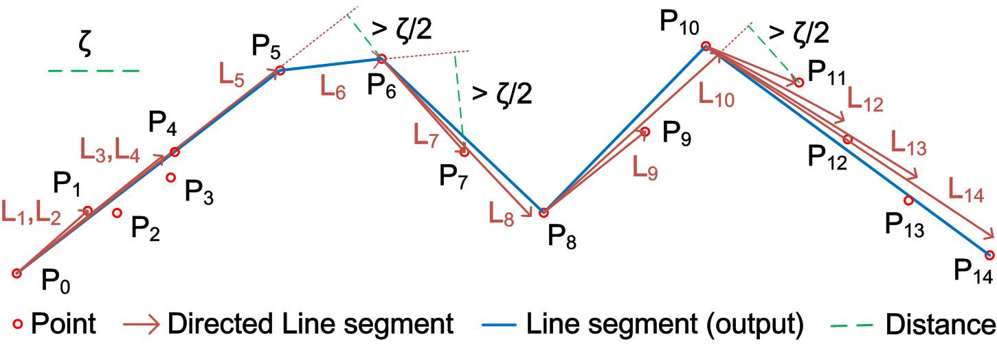
Figure 8: A running example of algorithm $\mathsf{OPERB}$.

4.4 Optimization Techniques

We further propose five optimization techniques for $\mathsf{OPERB}$ to achieve a better compression ratio. The key idea behind this is to (1) compress as many points as possible with a directed line segment, or (2) to let the directed line segment $\mathcal{L}_{i}$ as close as possible to the current active point $P_{i}$ so that it has a higher possibility to represent $P_{i+1}$. These optimization techniques are organized by the processing order from the start to the end points of directed line segments.

(1) Choosing the first active point after $P_{s}$. Algorithm $\mathsf{OPERB}$ calls procedure ${\mathsf{getActivePoint}}$ to get the first active point $P_{a}$ in a sub-trajectory $\dddot{\mathcal{T}}[P_{s+1},\ldots,$ $P_{s+k}]$ such that $|\vv{P_{s}P_{a}}|>\zeta/4$ (line 4 in Figure 7). However, as indicated by the fitting function $\mathbb{F}$, we can replace $P_{a}$ with the first point $P_{b}$ such that $|\vv{P_{s}P_{b}}|>\zeta$, without affecting the boundness of algorithm $\mathsf{OPERB}$. This method potentially improves the compression ratio because more points are covered by the directed line segment $\vv{P_{s}P_{b}}$ than $\vv{P_{s}P_{a}}$, and $\vv{P_{s}P_{b}}$ is also closer to $P_{b}$ than $\vv{P_{s}P_{a}}$.

(2) Adjusting the distance condition. Given any sub trajectory $\dddot{\mathcal{T}}[P_{s},\ldots,P_{s+k}]$ and error bound $\zeta$, let $d^{+}_{max}$ = $\max\{d(P_{s+i},\mathcal{L}_{i-1})\leavevmode\nobreak\ |\leavevmode\nobreak\ f(\mathcal{R}_{i},\mathcal{L}_{i-1})=1\leavevmode\nobreak\ and\leavevmode\nobreak\ i\in[1,k]\}$ and $d^{-}_{max}$ = $\max\{d(P_{s+i},\mathcal{L}_{i-1})\leavevmode\nobreak\ |\leavevmode\nobreak\ f(\mathcal{R}_{i},\mathcal{L}_{i-1})=-1\leavevmode\nobreak\ and\leavevmode\nobreak\ i\in[s+1,s+k]\}$. Then the condition $d(P_{s+i},\mathcal{L}_{i-1})\leq\zeta/2$ in Theorem 4.2 can be replaced with $d^{-}_{max}+d^{+}_{max}\leq\zeta$, and algorithm $\mathsf{OPERB}$ remains error bounded by $\zeta$. Say, if $d^{+}_{max}=0.3\zeta$ and $d^{-}_{max}=0.6\zeta$, then $d(P_{s+i},\mathcal{L}_{k})$ for each $i\in[s,s+k]$ is still less than $0.3\zeta+0.6\zeta=0.9\zeta<\zeta$.

Note that $d(P_{s+i},\mathcal{L}_{i-1})\leq\zeta/2$ implies $d^{+}_{max}\leq\zeta/2$ and $d^{-}_{max}\leq\zeta/2$, and, hence, $d^{-}_{max}+d^{+}_{max}\leq\zeta$. Therefore, $d(P_{s+i},\mathcal{L}_{i-1})\leq\zeta/2$ is a special case of $d^{-}_{max}+d^{+}_{max}\leq\zeta$.

(3) Making $\mathcal{L}$ more close to the active points. When $\mathsf{OPERB}$ calculates the angle $\mathcal{L}_{i}.\theta$ of an active point $P_{i}$, the factor $d(P_{i},\mathcal{L}_{i-1})$ in the fitting function $\mathbb{F}$ can be replaced by a bigger number $d_{x}$ such that $0\leq d_{x}\leq d^{-}_{max}$ when $f(\mathcal{R}_{i},\mathcal{L}_{i-1})=-1$ or $0\leq d_{x}\leq d^{+}_{max}$ when $f(\mathcal{R}_{i},\mathcal{L}_{i-1})=1$, to let $\mathcal{L}_{i}$ be more close to $P_{i}$, under the restriction that $(\arcsin(\frac{d_{x}}{j*\zeta/2})/j)$ is not larger than $\arcsin(\frac{d(P_{i},\mathcal{L}_{i-1})}{j*\zeta/2})$.

(4) Incorporating missing active points. For a sub-trajectory $\dddot{\mathcal{T}}[P_{s}$, $\ldots,P_{a},\ldots,P_{a+i},\ldots,P_{s+k}]$, whereas $P_{a}$ and $P_{a+i}$ are two consecutive active points. Let $j_{a}$ = $\lceil(|\mathcal{R}_{a}|*2/\zeta-0.5)\rceil$, $j_{a+1}$ = $\lceil(|\mathcal{R}_{a+i}|*2/\zeta-0.5)\rceil$ and $\Delta j=j_{a+1}-j_{a}$. If $\Delta j>1$, then there are no active points between zones $Z_{j_{a}}$ and $Z_{j_{a+1}}$. In this case, we replace $\mathcal{L}_{a+i}.\theta$ with $\mathcal{L}_{a+i-1}.\theta+f(\mathcal{R}_{a+i},\mathcal{L}_{a+i-1})*\arcsin(\frac{d(P_{a+i},\mathcal{L}_{a+i-1})}{j_{a+1}*\zeta/2})*\frac{\Delta j}{j_{a+1}}$ for the fitting function $\mathbb{F}$, instead of $\mathcal{L}_{a+i-1}.\theta+f(\mathcal{R}_{a+i},\mathcal{L}_{a+i-1})*\arcsin(\frac{d(P_{a+i},\mathcal{L}_{a+i-1})}{j_{a+1}*\zeta/2})*\frac{1}{j_{a+1}}$ to compensate the side effects of missing active points to make the line $\mathcal{L}_{a+i}$ more closer to $P_{a+i}$. Note that $\mathcal{L}_{a+i-1}=\mathcal{L}_{a}$ and $\Delta j>0$. Moreover, $d(P_{a+i},\mathcal{L}_{a+i-1})$ could also be replaced by $d_{x}$ as above.

(5) Absorbing data points after $P_{s+k}$. Given any sub-trajectory $\dddot{\mathcal{T}_{s}}[P_{s},\ldots,P_{s+k},\ldots,P_{s+t}]$ and error bound $\zeta$, if $[P_{s},\ldots,P_{s+k}]$ is compressed to a line segment $\vv{P_{s}P_{s+k}}$, then any point $P_{s+t}$ ($t>k$) can also be compressed to $\vv{P_{s}P_{s+k}}$ as long as $d(P_{s+t},{\vv{P_{s}P_{s+k}}})\leq\zeta$ such that $\mathsf{OPERB}$ can compress more points into the directed line segment.

Remark. These optimization techniques are seamlessly integrated into $\mathsf{OPERB}$, and Theorem 4.3 remains intact.

5 An Aggressive Approach

In this section, we introduce an aggressive one-pass trajectory simplification algorithm, referred to as $\mathsf{OPERB}$-$\mathsf{A}$, which extends algorithm $\mathsf{OPERB}$ by further allowing trajectory interpolation under certain conditions, and even achieves a better compression ratio than algorithm $\mathsf{DP}$, the existing $\mathsf{LS}$ algorithm with the best compression ratio.

5.1 Trajectory Interpolation

Existing line simplification algorithms, even the global distance checking algorithm $\mathsf{DP}$ and our algorithm $\mathsf{OPERB}$, may generate a set of anomalous line segments.

Anomalous line segments. Consider a trajectory $\dddot{\mathcal{T}}$$[P_{0},$ $\ldots,P_{n}]$ and its piece-wise line representation $\overline{\mathcal{T}}[\mathcal{R}_{0},$ $\ldots,\mathcal{R}_{m}]$ ($0<m\leq n$) generated by an $\mathsf{LS}$ algorithm. A line segment $\mathcal{R}_{i}$ ($i\in[0,m]$) is anomalous if it only represents two data points in $\dddot{\mathcal{T}}$, i.e., its own start and end points.

Anomalous line segments impair the effectiveness of trajectory simplification. We illustrate this with an example.

Example 5.13.

Let us consider the compressing results of algorithms $\mathsf{DP}$ and $\mathsf{OPERB}$ on a sub-trajectory, shown in Figure 9, which has one crossroad between data points $P_{3}$ and $P_{4}$, and another crossroad between data points $P_{7}$ and $P_{8}$. Given the sub-trajectory and the error bound as shown in Figure 9, algorithm $\mathsf{DP}$ returns four directed line segments $\{\vv{P_{0}P_{3}}$, $\vv{P_{3}P_{4}}$, $\vv{P_{4}P_{7}}$, $\vv{P_{7}P_{10}}\}$, and algorithm $\mathsf{OPERB}$ outputs five directed line segments $\{\vv{P_{0}P_{3}}$, $\vv{P_{3}P_{4}}$, $\vv{P_{4}P_{7}}$, $\vv{P_{7}P_{8}}$, $\vv{P_{8}P_{10}}\}$, respectively. Observe that the directed line segments $\vv{P_{3}P_{4}}$ and $\vv{P_{7}P_{8}}$ are anomalous.

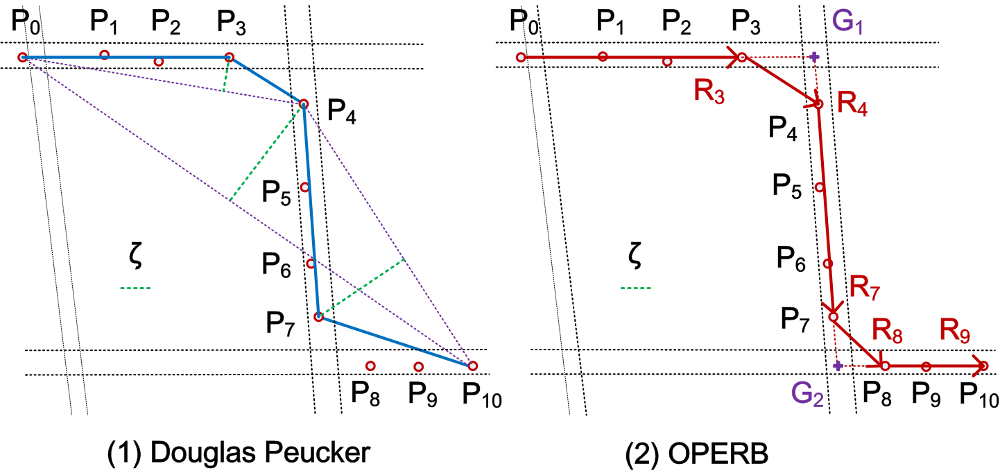
Figure 9: Example anomalous line segments: the compression results of algorithms $\mathsf{DP}$ and $\mathsf{OPERB}$ on a sub-trajectory with eleven points collected from a moving vehicle running on an urban road network.

In this work, we propose the use of interpolating new data points, referred to as patch points, into a trajectory under certain conditions to reduce the number of anomalous line segments to a large extent. The rational behind this is that moving objects have sudden track changes while certain important data points may not be sampled due to various reasons, especially on urban road networks. Note that slightly changing the lines has proven useful in other disciplines [17].

Patch points. Let $\mathcal{R}_{i-1}$, $\mathcal{R}_{i}$ and $\mathcal{R}_{i+1}$ be three continuous directed line segments, where $\mathcal{R}_{i}$ is anomalous, i.e., $\mathcal{R}_{i}$ represents only two points. The patch point $G$ w.r.t. $\mathcal{R}_{i}$ is the intersection point between line segments $\mathcal{R}_{i-1}$ and $\mathcal{R}_{i+1}$.

We next illustrate the use of patch points for reducing anomalous line segments with an example.

Example 5.14.

Consider Figure 9(2), where $G_{1},G_{2}$ are the patch points w.r.t. $\mathcal{R}_{4}$ and $\mathcal{R}_{8}$, respectively. After $G_{1}$ and $G_{2}$ are interpolated, both algorithms $\mathsf{DP}$ and $\mathsf{OPERB}$ return three directed line segments $\{\vv{P_{0}G_{1}}$, $\vv{G_{1}G_{2}}$, $\vv{G_{2}P_{10}}\}$, instead of four and five, respectively, as shown in Example 5.13.

Patching method. Consider any three continuous directed line segments, $\mathcal{R}_{i-1}=\vv{P_{s}P_{s+i-1}}$, $\mathcal{R}_{i}=\vv{P_{s+i-1}P_{s+i}}$ and $\mathcal{R}_{i+1}$ $=$ $\vv{P_{s+i}P_{t}}$ such that $\mathcal{R}_{i}$ is anomalous and point $P_{t}$ is an active point and $t>s+i$. With the practical restrictions and one-pass requirement, the patch point $G$ w.r.t. $\mathcal{R}_{i}$ needs to satisfy the conditions below, as illustrated by Figure 10.

(1) Lying on the lines of $\vv{P_{s}P_{s+i-1}}$ (i.e., $\vv{P_{s}G}.\theta=\vv{P_{s}P_{s+i-1}}.\theta$) and $\vv{P_{s+i}P_{t}}$ (i.e., $\vv{GP_{s+i}}.\theta=\vv{P_{s+i}P_{t}}.\theta$),

(2) $|\vv{P_{s}G}|\geq(|\vv{P_{s}P_{s+i-1}}|-\zeta/2)$, and

(3) the included angle from $\mathcal{R}_{i-1}$ to $\mathcal{R}_{i+1}$ falls in $(-2\pi,-\pi-\gamma_{m}]$, $[\gamma_{m}-\pi,\pi-\gamma_{m}]$ and $[\pi+\gamma_{m},2\pi)$, where $\gamma_{m}\in[0,\pi]$ is a parameter with $\gamma_{m}=\frac{\pi}{3}$ by default.

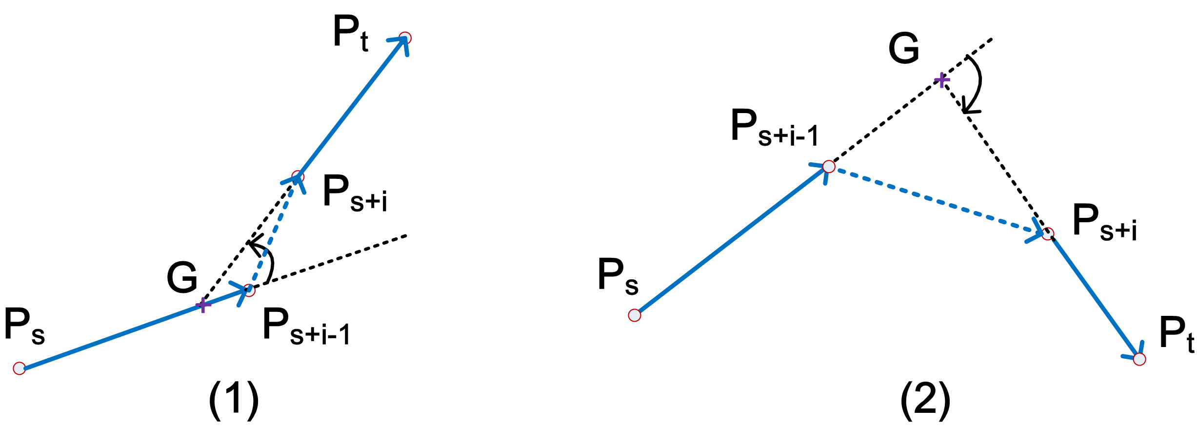
Figure 10: Practical restrictions on patch points.

Intuitively, these conditions are to incorporate the sudden changes of moving directions implied in a trajectory. Note that the restriction of the included angles may reduce the chance of eliminating anomalous line segments. However, it helps to produce more rational results.

5.2 Algorithm OPERB–A

We now present our algorithm $\mathsf{OPERB}$-$\mathsf{A}$ that extends algorithm $\mathsf{OPERB}$ by introducing patch points. Recall that algorithm $\mathsf{OPERB}$ starts a new directed line segment when the distance of a point, say $P_{i}$, to the line segment $\mathcal{L}_{i-1}$ is larger than $\zeta/2$, marks the last active point $P_{a}$ as $P_{s+i-1}$, outputs the directed line segment $\mathcal{R}_{i-1}=\vv{P_{s}P_{s+i-1}}$, and marks $P_{s+i-1}$ as the new start point $P_{s}$ of the remaining subjectify $\dddot{\mathcal{T}_{s}}[P_{s+i-1},\ldots,P_{n}]$. However, for $\mathsf{OPERB}$-$\mathsf{A}$, the line segment $\mathcal{R}_{i-1}$ cannot be outputted until the patch point $G$ is determined when $R_{i}=\vv{P_{s+i-1}P_{s+i}}$ is an $\mathsf{AL}$, and patch point $G$ cannot be determined unless the angle of $\mathcal{R}_{i+1}=\vv{P_{s+i}P_{t}}$ has been determined. Hence, different from $\mathsf{OPERB}$, $\mathsf{OPERB}$-$\mathsf{A}$ uses a lazy output policy.

The lazy output policy. $\mathsf{OPERB}$-$\mathsf{A}$ temporarily saves a line segment in memory before outputting it, as follows:

(1) For simplicity, suppose that the line segment $\mathcal{R}_{i-1}$ is not anomalous and cannot be compressed with any more points. $\mathsf{OPERB}$-$\mathsf{A}$ saves it in memory first.

(2) It then compresses the subsequent points as $\mathsf{OPERB}$ to the next line segment $\mathcal{R}_{i}$ until a broken condition is triggered. If $\mathcal{R}_{i}$ is not anomalous, then it outputs $\mathcal{R}_{i-1}$ and saves $\mathcal{R}_{i}$ in memory. Otherwise, it marks $\mathcal{R}_{i}$ anomalous, saves it, and moves to the next line segment $\mathcal{R}_{i+1}$.

(3) If $\mathcal{R}_{i+1}$ is determined and $\mathcal{R}_{i}$ is anomalous, $\mathsf{OPERB}$-$\mathsf{A}$ checks the possibility of patching a point $G$ w.r.t. $\mathcal{R}_{i}$. If so, it outputs $\vv{P_{s}G}$, and $\vv{GP_{t}}$ is temporarily saved; Otherwise, it outputs $\mathcal{R}_{i-1}$ and $\mathcal{R}_{i}$, and $\mathcal{R}_{i+1}$ is temporarily saved.

(4) The process repeats until all points have been processed.

Remarks. All the optimization techniques in Section 4.4 remain intact, and are seamlessly integrated into $\mathsf{OPERB}$-$\mathsf{A}$.

We next explain algorithm $\mathsf{OPERB}$-$\mathsf{A}$ with an example.

Example 5.15.

Algorithm $\mathsf{OPERB}$-$\mathsf{A}$ takes as input the trajectory and $\zeta$ shown in Figure 1, and its output is illustrated in Figure 11. The process of $\mathsf{OPERB}$-$\mathsf{A}$ is as follows.

(1) It first creates $\mathcal{L}_{0}=\mathcal{R}_{0}=\vv{P_{0}P_{0}}$, compresses $P_{1}$, …, $P_{5}$ in turn, and generates $\mathcal{L}_{5}$, along the same lines as $\mathsf{OPERB}$.

(2) It then finds that $d(P_{6},\mathcal{L}_{5})>\zeta/2$, which means that $P_{6}$ cannot be compressed into $\mathcal{R}_{5}=\vv{P_{0}P_{5}}$. $\mathcal{R}_{5}$ is temporally saved. And the next line segment starts from $P_{5}$.

(3) It then finds that $d(P_{7},\mathcal{L}_{6})>\zeta/2$ and $\mathcal{R}_{6}=\vv{P_{5}P_{6}}$ is an $\mathsf{AL}$. Hence, $\mathcal{R}_{6}$ is also temporally saved, and the next line segment starts from $P_{6}$.

(4) It continues to compress points $P_{7}$ and $P_{8}$ in turn, and generates $\mathcal{L}_{8}$ along the same lines as $\mathsf{OPERB}$.

(5) It then finds that $d(P_{9},\mathcal{L}_{8}))>\zeta/2$, which means that $\mathcal{R}_{8}=\vv{P_{6}P_{8}}$ is determined. Now $\mathsf{OPERB}$-$\mathsf{A}$ tries to expand the lines of $\mathcal{R}_{5}$ and $\mathcal{R}_{8}$ to get the intersection point $G$ of them, and uses it as the final start point of $\mathcal{R}_{8}$. At last, $\mathcal{R}_{5}$ is extended to $\vv{P_{0}G}$ and output as a directed line segment in the result, $\vv{GP_{8}}$ is temporarily saved and $P_{8}$ becomes the start point of the next line segment.

(6) The above process repeats until all points have been processed. Finally, $\mathsf{OPERB}$-$\mathsf{A}$ outputs four line segments $\{\vv{P_{0}G}$, $\vv{GP_{8}}$, $\vv{P_{8}P_{10}}$, $\vv{P_{10}P_{14}}\}$.

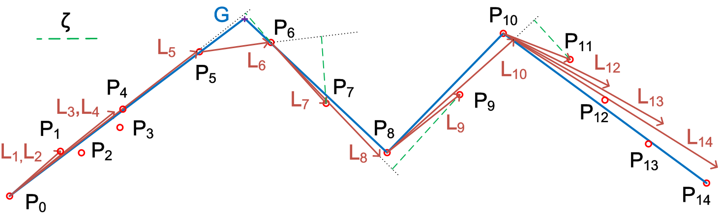
Figure 11: A running example of $\mathsf{OPERB}$-$\mathsf{A}$.

As shown in Figure 11, algorithm $\mathsf{OPERB}$-$\mathsf{A}$ further eliminates the directed line segment $\vv{P_{5}P_{6}}$, compared with the result of $\mathsf{OPERB}$ shown in Figure 8.

Correctness & complexity analysis. Observe that algorithm $\mathsf{OPERB}$-$\mathsf{A}$ does not change the angle of any directed line segment compared with $\mathsf{OPERB}$, and hence it remains error bounded. Moreover, each data point in a trajectory is read once and only once in $\mathsf{OPERB}$-$\mathsf{A}$. Therefore, algorithm $\mathsf{OPERB}$-$\mathsf{A}$ is one-pass and error bounded. It is also easy to verify that algorithm $\mathsf{OPERB}$-$\mathsf{A}$ takes $O(1)$ space, the same as $\mathsf{OPERB}$, as the directed line segment in $\overline{\mathcal{T}}$ can be outputted immediately once it is generated. That is, the nice properties of $\mathsf{OPERB}$ remain intact in $\mathsf{OPERB}$-$\mathsf{A}$.

6 Experimental Study

In this section, we present an extensive experimental study of our one-pass error bounded algorithms $\mathsf{OPERB}$ and $\mathsf{OPERB}$-$\mathsf{A}$. Using four real-life datasets, we conducted four sets of experiments to evaluate: (1) the execution time of our approaches compared with algorithms $\mathsf{DP}$ and $\mathsf{FBQS}$, and the impacts of optimizations, (2) the compression ratios of our approaches compared with $\mathsf{DP}$ and $\mathsf{FBQS}$, and the impacts of optimizations, (3) the average errors of our approaches compared with algorithms $\mathsf{DP}$ and $\mathsf{FBQS}$, and (4) the effectiveness of trajectory interpolation.

6.1 Experimental Setting

Real-life Trajectory Datasets. We use four real-life datasets shown in Table 1 to test our solutions.

(1) Taxi trajectory data, referred to as $\mathsf{Taxi}$, is the GPS trajectories collected by $12,727$ taxies equipped with GPS sensors in Beijing during a period from Nov. 1, 2010 to Nov. 30, 2010. The sampling rate was one point per 60s, and $\mathsf{Taxi}$ has $39,100$ data points on average per trajectory.

(2) Truck trajectory data, referred to as $\mathsf{Truck}$, is the GPS trajectories collected by 10,368 trucks equipped with GPS sensors in China during a period from Mar. 2015 to Oct. 2015. The sampling rate varied from 1s to 60s. Trajectories mostly have around $50$ to $90$ thousand data points.

(3) Service car trajectory data, referred to as $\mathsf{SerCar}$, is the GPS trajectories collected by a car rental company. We chose $11,000$ cars from them, during Apr. 2015 to Nov. 2015. The sampling rate was one point per $3$–$5$ seconds, and each trajectory has around $119.1K$ data points.

(4) GeoLife trajectory data, refered to as $\mathsf{GeoLife}$, is the GPS trajectories collected in GeoLife project [25] by 182 users in a period from Apr. 2007 to Oct. 2011. These trajectories have a variety of sampling rates, among which 91% are logged in each 1-5 seconds or each 5-10 meters per point. The longest trajectory has 2,156,994 points.

$\mathsf{Data}$	$\mathsf{Number\ of}$	$\mathsf{Sampling}$	$\mathsf{PointsPer}$	$\mathsf{Total}$
$\mathsf{Sets}$	$\mathsf{Trajectories}$	$\mathsf{Rates(s)}$	$\mathsf{Trajectory(K)}$	$\mathsf{points}$
$\mathsf{Taxi}$	12,727	60	$\sim 39.1$	498M
$\mathsf{Truck}$	10,368	1-60	$\sim 71.9$	746M
$\mathsf{SerCar}$	11,000	3-5	$\sim 119.1$	1.31G
$\mathsf{GeoLife}$	182	1-5	$\sim 132.8$	24.2M

Table 1: Real-life trajectory datasets

Algorithms and implementation. We compared our algorithms $\mathsf{OPERB}$ and $\mathsf{OPERB}$-$\mathsf{A}$ with two existing $\mathsf{LS}$ algorithms $\mathsf{DP}$ [6] and $\mathsf{FBQS}$ [12], and algorithms $\mathsf{Raw}$-$\mathsf{OPERB}$ and $\mathsf{Raw}$-$\mathsf{OPERB}$-$\mathsf{A}$, the counterparts of $\mathsf{OPERB}$ and $\mathsf{OPERB}$-$\mathsf{A}$ without optimizations, respectively.

(1) Algorithm $\mathsf{DP}$ is a classic batch $\mathsf{LS}$ algorithm with an excellent compression ratio (shown in Figure 3).

(2) Algorithm $\mathsf{FBQS}$ is an online algorithm, and is the fastest existing $\mathsf{LS}$ algorithm (recall Section 3.2).

(3) Algorithm $\mathsf{OPERB}$ combines the algorithm in Figure 7 and the optimization techniques in Section 4.4, while algorithm $\mathsf{Raw}$-$\mathsf{OPERB}$ is the basic algorithm in Figure 7 only.

(4) Algorithms $\mathsf{OPERB}$-$\mathsf{A}$ and $\mathsf{Raw}$-$\mathsf{OPERB}$-$\mathsf{A}$ are the aggressive solutions extending $\mathsf{OPERB}$ and $\mathsf{Raw}$-$\mathsf{OPERB}$ with trajectory interpolation, respectively.

All algorithms were implemented with Java. All tests were run on an x64-based PC with 4 Intel(R) Core(TM) i5-4570 CPU @ 3.20GHz and 16GB of memory, and each test was repeated over 3 times and the average is reported here.

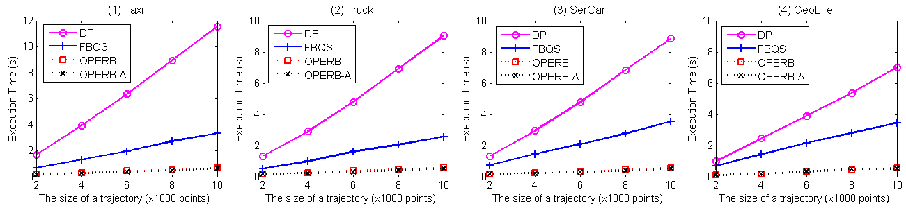
Figure 12: Efficiency evaluation: varying the size of trajectories.

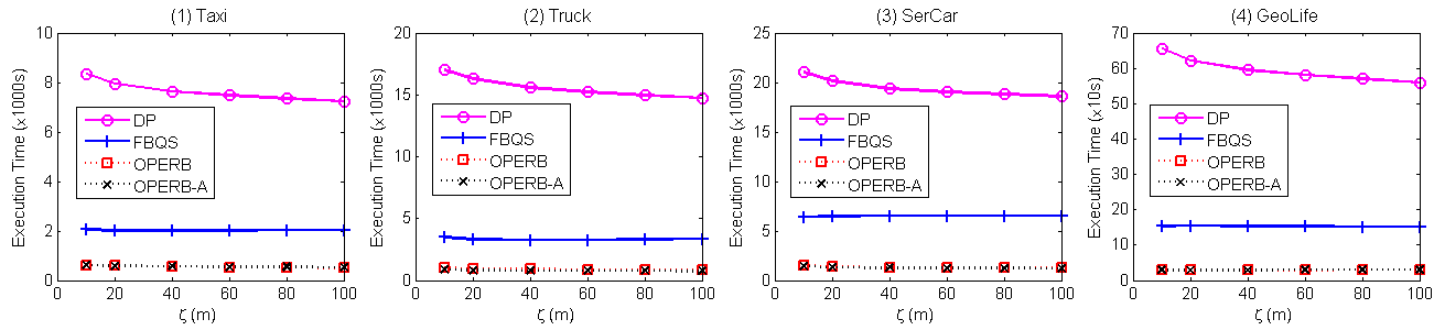
Figure 13: Efficiency evaluation: varying the error bound $\zeta$.

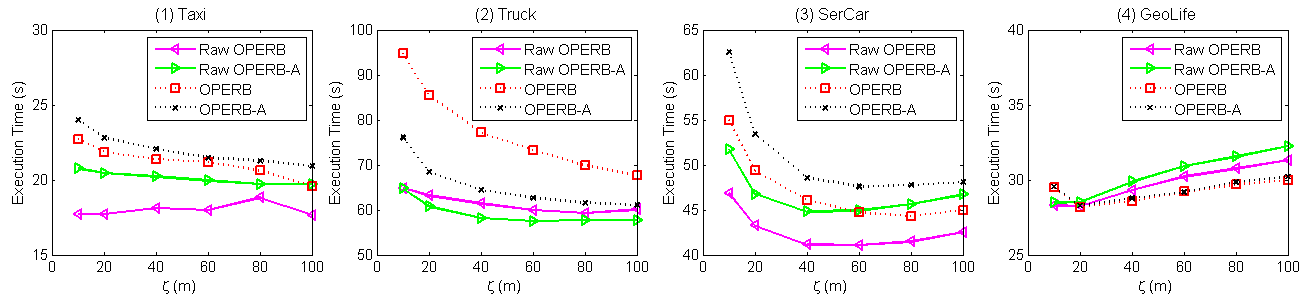
Figure 14: Efficiency evaluation: optimization techniques when varying the error bound $\zeta$.

6.2 Experimental Results

6.2.1 Evaluation of Compression Efficiency

In the first set of tests, we compare the efficiency (execution time) of our approaches $\mathsf{OPERB}$ and $\mathsf{OPERB}$-$\mathsf{A}$ with algorithms $\mathsf{DP}$ and $\mathsf{FBQS}$ and with algorithms $\mathsf{Raw}$-$\mathsf{OPERB}$ and $\mathsf{Raw}$-$\mathsf{OPERB}$-$\mathsf{A}$. For fairness, we load and compress trajectories one by one, and only count the running time of the compressing process.

Exp-1.1: Impacts of the sizes of trajectories. To evaluate the impacts of the number of data points in a trajectory (i.e., the size of a trajectory), we chose $100$ trajectories from $\mathsf{Taxi}$, $\mathsf{Truck}$, $\mathsf{SerCar}$ and $\mathsf{GeoLife}$, respectively, and varied the size $\dddot{\mathcal{|T|}}$ of trajectories from $2,000$ to $10,000$, while fixed $\zeta=40$ meters (m). The results are reported in Figure 12.

(1) Algorithms $\mathsf{OPERB}$, $\mathsf{OPERB}$-$\mathsf{A}$ and $\mathsf{FBQS}$ scale well with the increase of the size of trajectories on all datasets, and show a linear running time, while algorithm $\mathsf{DP}$ does not. This is consistent with their time complexity analyses.

(2) Algorithms $\mathsf{OPERB}$ and $\mathsf{OPERB}$-$\mathsf{A}$ are the fastest $\mathsf{LS}$ algorithms, and are ($3.8$–$5.3$, $3.5$–$4.8$, $4.6$–$7.2$, $6.2$–$8.4$) times faster than $\mathsf{FBQS}$, and ($9.6$–$17.6$, $8.8$–$15.4$, $8.4$–$16.3$, $9.0$–$14.4$) times faster than $\mathsf{DP}$ on ($\mathsf{Taxi}$, $\mathsf{Truck}$, $\mathsf{SerCar}$, $\mathsf{GeoLife}$), respectively. The running time of $\mathsf{OPERB}$ and $\mathsf{OPERB}$-$\mathsf{A}$ is similar, and the difference is below 10%.

Exp-1.2: Impacts of the error bound $\zeta$. To evaluate the impacts of $\zeta$, we varied $\zeta$ from $10m$ to $100m$ on the entire $\mathsf{Taxi}$, $\mathsf{Truck}$, $\mathsf{SerCar}$ and $\mathsf{GeoLife}$, respectively. The results are reported in Figure 13.

(1) All algorithms are not very sensitive to $\zeta$, but their running time all decreases a little bit with the increase of $\zeta$, as the increment of $\zeta$ decreases the number of directed line segments in the output. Further, algorithm $\mathsf{DP}$ is more sensitive to $\zeta$ than the other three algorithms.

(2) Algorithms $\mathsf{OPERB}$ and $\mathsf{OPERB}$-$\mathsf{A}$ are obviously faster than $\mathsf{DP}$ and $\mathsf{FBQS}$ in all cases. $\mathsf{OPERB}$ is on average ($13.9$, $17.4$, $14.7$, $20.6$) times faster than $\mathsf{DP}$, and ($4.1$, $4.1$, $5.4$, $5.2$) times faster than $\mathsf{FBQS}$ on ($\mathsf{Taxi}$, $\mathsf{Truck}$, $\mathsf{SerCar}$, $\mathsf{GeoLife}$), respectively. Algorithm $\mathsf{OPERB}$-$\mathsf{A}$ is as fast as $\mathsf{OPERB}$ because trajectory interpolation is a light weight operation.

Exp-1.3: Impacts of optimization techniques. To evaluate the impacts of our optimization techniques (see Section 4.4), we compared algorithms $\mathsf{OPERB}$ and $\mathsf{OPERB}$-$\mathsf{A}$ with $\mathsf{Raw}$-$\mathsf{OPERB}$ and $\mathsf{Raw}$-$\mathsf{OPERB}$-$\mathsf{A}$, respectively. We chose $500$, $1000$ and $500$ trajectories from $\mathsf{Taxi}$, $\mathsf{Truck}$, $\mathsf{SerCar}$ and $\mathsf{GeoLife}$, respectively, and varied $\zeta$ from 10m to 100m. The results are reported in Figure 14.

(1) The running time of all algorithms slightly decreases with the increase of $\zeta$, consistent with Exp-1.2.

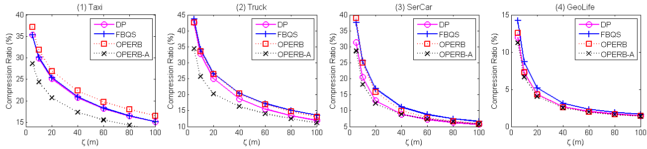
Figure 15: Effectiveness evaluation: varying the error bound $\zeta$.

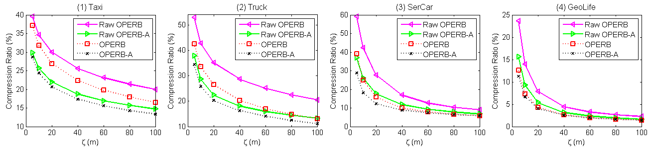
Figure 16: Effectiveness evaluation: optimization techniques when varying the error bound $\zeta$.

(2) The running time of $\mathsf{Raw}$-$\mathsf{OPERB}$ is $(85.0\%$, $79.6\%$, $90.4\%$, $100.4\%$) of $\mathsf{OPERB}$ on average on (${\mathsf{Taxi}}$, ${\mathsf{Truck}}$, ${\mathsf{SerCar}}$, ${\mathsf{GeoLife}}$), respectively, and the running time of $\mathsf{Raw}$-$\mathsf{OPERB}$-$\mathsf{A}$ is $(91.3\%$, $90.1\%$, $91.6\%$, $101.5\%$) of $\mathsf{OPERB}$-$\mathsf{A}$ on average on (${\mathsf{Taxi}}$, ${\mathsf{Truck}}$, ${\mathsf{SerCar}}$, ${\mathsf{GeoLife}}$), respectively. This shows that the optimization techniques have a limited impact on the efficiency of $\mathsf{OPERB}$ and $\mathsf{OPERB}$-$\mathsf{A}$. However, as will be shown immediately, the benefits of compression ratios are highly appreciated.

6.2.2 Evaluation of Compression Effectiveness

In the second set of tests, we compare the compression ratios of our algorithms $\mathsf{OPERB}$ and $\mathsf{OPERB}$-$\mathsf{A}$ with $\mathsf{DP}$ and $\mathsf{FBQS}$ and with $\mathsf{Raw}$-$\mathsf{OPERB}$ and $\mathsf{Raw}$-$\mathsf{OPERB}$-$\mathsf{A}$, respectively. Given a set of trajectories $\{\dddot{\mathcal{T}_{1}},\ldots,\dddot{\mathcal{T}_{M}}\}$ and their piecewise line representations $\{\overline{\mathcal{T}_{1}},\ldots,\overline{\mathcal{T}_{M}}\}$, the compression ratio is $(\sum_{j=1}^{M}|\overline{\mathcal{T}}_{j}|)/(\sum_{j=1}^{M}|\dddot{\mathcal{T}}_{j}|)$. Note that by the definition, algorithms with lower compression ratios are better.

Exp-2.1: Impacts of the error bound $\zeta$. To evaluate the impacts of $\zeta$ on compression ratios of these algorithms, we varied $\zeta$ from $5m$ to $100m$ on the entire four datasets, respectively. The results are reported in Figure 15.

(1) When increasing $\zeta$, the compression ratios decrease. For example, in $\mathsf{SerCar}$, the compression ratios are greater than $28.7\%$ when $\zeta$ = $5m$, but are less than $6.6\%$ when $\zeta$ = $100m$.

(2) $\mathsf{GeoLife}$ has the lowest compression ratios, compared with $\mathsf{Taxi}$, $\mathsf{Truck}$ and $\mathsf{SerCar}$, due to its highest sampling rate, $\mathsf{Taxi}$ has the highest compression ratios due to its lowest sampling rate, and $\mathsf{Truck}$ and $\mathsf{SerCar}$ have the compression ratios in the middle accordingly.

(3) First, algorithm $\mathsf{OPERB}$ has comparable compression ratios with $\mathsf{FBQS}$ and $\mathsf{DP}$. For example, when $\zeta=40m$, the compression ratios are ($20.9\%$, $20.4\%$, $11.1\%$, $3.1\%$) of $\mathsf{FBQS}$, ($20.7\%$, $18.7\%$, $8.9\%$, $2.6\%$) of $\mathsf{DP}$ and ($22.3\%$, $20.3\%$, $10.0\%$, $2.6\%$) of $\mathsf{OPERB}$ on ($\mathsf{Taxi}$, $\mathsf{Truck}$, $\mathsf{SerCar}$, $\mathsf{GeoLife}$), respectively. For all $\zeta$, the compression ratios of $\mathsf{OPERB}$ are on average ($107.2\%$, $98.3\%$, $92.9\%$, $85.1\%$) of $\mathsf{FBQS}$ and ($107.7\%$, $106.6\%$, $113.5\%$, $99.6\%$) of $\mathsf{DP}$ on ($\mathsf{Taxi}$, $\mathsf{Truck}$, $\mathsf{SerCar}$, $\mathsf{GeoLife}$), respectively. $\mathsf{OPERB}$ is better than $\mathsf{FBQS}$ on $\mathsf{Truck}$, $\mathsf{SerCar}$ and $\mathsf{GeoLife}$, while a little worse on $\mathsf{Taxi}$. The results also show that $\mathsf{OPERB}$ has a better performance than $\mathsf{FBQS}$ on datasets with high sampling rates.

Second, algorithm $\mathsf{OPERB}$-$\mathsf{A}$ achieves the best compression ratios on all datasets and nearly all $\zeta$ values. Its compression ratios are on average ($83.7\%$, $79.5\%$, $79.7\%$, $81.0\%$) of $\mathsf{FBQS}$ and ($84.2\%$, $86.4\%$, $97.1\%$, $94.7\%$) of $\mathsf{DP}$ on ($\mathsf{Taxi}$, $\mathsf{Truck}$, $\mathsf{SerCar}$, $\mathsf{GeoLife}$), respectively. Similar to $\mathsf{OPERB}$, $\mathsf{OPERB}$-$\mathsf{A}$ has advantages on datasets with high sampling rates.

Exp-2.2: Impacts of the optimization techniques. We compared algorithms $\mathsf{OPERB}$ and $\mathsf{OPERB}$-$\mathsf{A}$ with $\mathsf{Raw}$-$\mathsf{OPERB}$ and $\mathsf{Raw}$-$\mathsf{OPERB}$-$\mathsf{A}$, respectively. We varied $\zeta$ from $5m$ to $100m$ on the entire $\mathsf{Taxi}$, $\mathsf{Truck}$, $\mathsf{SerCar}$ and $\mathsf{GeoLife}$, respectively. The results are reported in Figure 16.

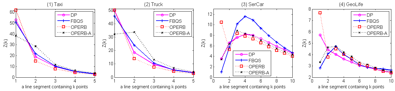
Figure 17: Effectiveness evaluation: distribution of line segments. The horizontal coordinate is the number $k$ of data points, and the vertical coordinate is the number $\mathcal{Z}(k)$ of line segments containing $k$ points.

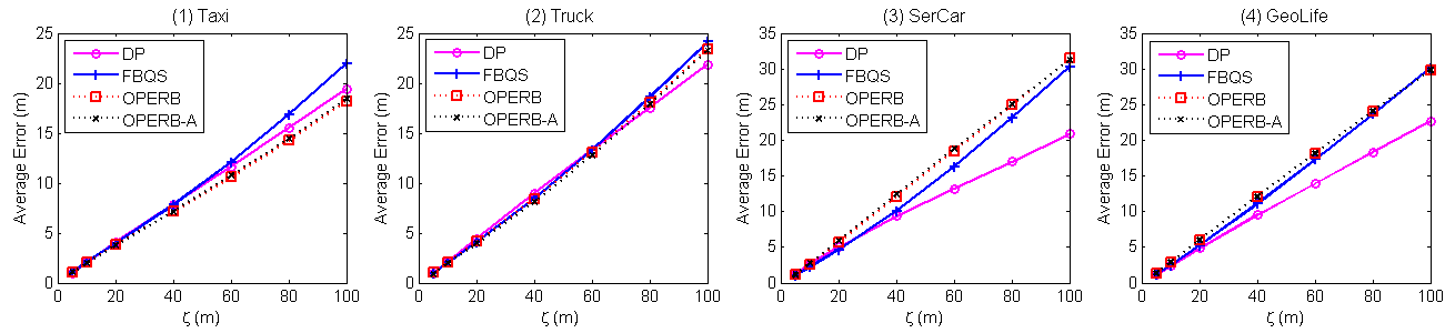
Figure 18: Evaluation of average errors: varying the error bound $\zeta$.

(1) The optimizations have great impacts on the compression ratios of $\mathsf{OPERB}$ and $\mathsf{OPERB}$-$\mathsf{A}$. Indeed, $\mathsf{OPERB}$ is on average ($87.9\%$, ${71.8\%}$, $61.8\%$, $58.0\%$) of $\mathsf{Raw}$-$\mathsf{OPERB}$, and $\mathsf{OPERB}$-$\mathsf{A}$ is on average ($93.1\%$, ${88.5\%}$, $77.1\%$, $78.5\%$) of $\mathsf{Raw}$-$\mathsf{OPERB}$-$\mathsf{A}$ on ($\mathsf{Taxi}$, $\mathsf{Truck}$, $\mathsf{SerCar}$, $\mathsf{GeoLife}$), respectively. Note that the optimization techniques have a better impact on datasets with high sampling rates.

(2) The impacts of the optimization techniques increase with the increase of $\zeta$ on $\mathsf{Taxi}$ and $\mathsf{Truck}$. For example, $\mathsf{OPERB}$ is ($92.1\%$, ${87.3\%}$, $82.6\%$) of $\mathsf{Raw}$-$\mathsf{OPERB}$ on $\mathsf{Taxi}$, and ($78.5\%$, $70.9\%$, $63.7\%$) of $\mathsf{Raw}$-$\mathsf{OPERB}$ on $\mathsf{Truck}$ when $\zeta$ = ($10$, $40$, $100$), respectively. It is similar for algorithm $\mathsf{OPERB}$-$\mathsf{A}$.

Exp-2.3: Distribution of line segments. To further evaluate the difference of the compression results of these algorithms, we chose $100$ trajectories from each of ($\mathsf{Taxi}$, $\mathsf{Truck}$, $\mathsf{SerCar}$, $\mathsf{GeoLife}$), while fixed $\zeta=40m$. For a $\overline{\mathcal{T}}$ = $(\mathcal{L}_{1},\mathcal{L}_{2},\cdots,\mathcal{L}_{M})$ derived from trajectories by a compression algorithm, we count the number of points, $C_{i}$, included in each $\mathcal{L}_{i}$, then let $\mathcal{Z}(k)=|\{C_{i}|C_{i}=k\}|$, i.e., $\mathcal{Z}(5)$ means the number of all $\mathcal{L}_{i}$ containing 5 data points. Note that the start/end points are repeatedly counted for adjacent line segments, and, hence, there may be some lines having only one point. The results are reported in Figure 17.

(1) Algorithms $\mathsf{OPERB}$-$\mathsf{A}$ and $\mathsf{DP}$ produce more line segments containing large number of points (heavy line segments) than $\mathsf{FBQS}$ and $\mathsf{OPERB}$. Heavy line segments are closely related to compression ratios, and help to decrease compression ratios. The distribution of line segments is consistent with the compression ratios shown above.

(2) Algorithm $\mathsf{OPERB}$ has the largest number of line segments containing only one point. However, they are reduced by $\mathsf{OPERB}$-$\mathsf{A}$ to a large extent.

6.2.3 Evaluation of Average Errors

In the third set of tests, we evaluate the average errors of these algorithms. We varied $\zeta$ from $5m$ to $100m$ on the entire $\mathsf{Taxi}$, $\mathsf{Truck}$, $\mathsf{SerCar}$ and $\mathsf{GeoLife}$, respectively. Given a set of trajectories $\{\dddot{\mathcal{T}_{1}},\ldots,\dddot{\mathcal{T}_{M}}\}$ and their piecewise line representations $\{\overline{\mathcal{T}_{1}},\ldots,\overline{\mathcal{T}_{M}}\}$, and point $P_{j,i}$ denoting a point in trajectory $\dddot{\mathcal{T}}_{j}$ contained in a line segment $\mathcal{L}_{l,i}\in\overline{\mathcal{T}_{l}}$ ($l\in[1,M]$), then the average error is $\sum_{j=1}^{M}\sum_{i=0}^{M}d(P_{j,i},\mathcal{L}_{l,i})/\sum_{j=1}^{M}{|\dddot{\mathcal{T}}_{j}|}$. The results are reported in Figure 18.

(1) Average errors obviously increase with the increase of $\zeta$. $\mathsf{Taxi}$ also has the lowest average errors than $\mathsf{Truck}$ and $\mathsf{SerCar}$ for all algorithms, as it has the highest compression ratios, and $\mathsf{SerCar}$ has the highest average errors, as it has the lowest compression ratios among the three datasets.

(2) Algorithm $\mathsf{DP}$ not only has better compression ratios, but also has lower average errors than algorithm $\mathsf{FBQS}$ on all datasets and most $\zeta$ values.

(3) Algorithms $\mathsf{OPERB}$ and $\mathsf{OPERB}$-$\mathsf{A}$ have similar average errors with each other. Meanwhile, $\mathsf{OPERB}$-$\mathsf{A}$ does not introduce extra error. Compared with $\mathsf{DP}$ and $\mathsf{FBQS}$, their errors are a litter smaller on $\mathsf{Taxi}$ and a little larger on $\mathsf{SerCar}$.

6.2.4 Evaluation of Trajectories Interpolation

In the last set of tests, we evaluate the lazy trajectory interpolation policy of algorithm $\mathsf{OPERB}$-$\mathsf{A}$.

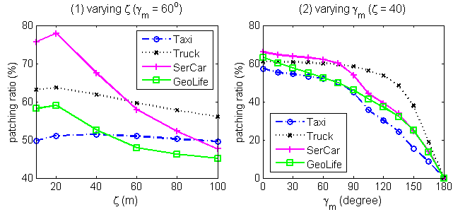
Figure 19: Patching ratios of $\mathsf{OPERB}$-$\mathsf{A}$.

Exp-4.1: Patching ratios. To evaluate the patching ratios of $\mathsf{OPERB}$-$\mathsf{A}$ and the impacts of $\zeta$ on patching ratios, we varied $\zeta$ from $10$m to $100$m, while fixed $\gamma_{m}=\pi/3$, on $\mathsf{Taxi}$, $\mathsf{Truck}$, $\mathsf{SerCar}$ and $\mathsf{GeoLife}$, respectively. The patching ratio is defined as $\frac{N_{p}}{N_{a}}*100\%$, where $N_{p}$ is the number of patching points successful added to the trajectories, and $N_{a}$ is the number of anonymous line segments before trajectory interpolation. The results are reported in Figure 19–(1).

(1) The patching ratios are on average ($50.5\%$, $60.3\%$, $63.2\%$, $51.5\%$) on ($\mathsf{Taxi}$, $\mathsf{Truck}$, $\mathsf{SerCar}$, $\mathsf{GeoLife}$), respectively. That is, more than half of the anomalous line segments are successfully eliminated by the lazy trajectory output policy.

(2) The patching ratios on $\mathsf{Taxi}$, $\mathsf{Truck}$, $\mathsf{SerCar}$ and $\mathsf{GeoLife}$ decrease from $\zeta=30m$ or $\zeta=40m$, respectively.

(3) $\mathsf{Taxi}$ has the lowest patching ratios due to its relatively lower sampling rate. Moreover, the number of anomalous line segments output by $\mathsf{OPERB}$-$\mathsf{A}$ is significantly less than the other algorithms. That is, even a patching ratio like 50.5% is enough to improve the compression ratio and to make $\mathsf{OPERB}$-$\mathsf{A}$ have the best compression ratio.

Exp-4.2: Impacts of $\gamma_{m}$ for trajectory interpolation. Our trajectory interpolation uses a parameter $\gamma_{m}\in[0,\pi]$ to restrict the included angle of two line segments. Note that a smaller $\gamma_{m}$ means that a larger direction change is allowed in trajectory interpolation. To evaluate the impacts of $\gamma_{m}$ on patching ratios, we randomly chose $100$ trajectories from each of ($\mathsf{Taxi}$, $\mathsf{Truck}$, $\mathsf{SerCar}$), and we varied $\gamma_{m}$ from $0^{o}$ to $180^{o}$ (or 0 to $\pi$), while fixed $\zeta=40m$. The results are reported Figure 19–(2).

(1) When varying $\gamma_{m}$, the patching ratio decreases with the increase of $\gamma_{m}$. The patching ratio decreases (a) slowly when $\gamma_{m}\in[0,75^{o}]$, (b) fast when $\gamma_{m}\in(75^{o},145^{o})$, and (c) fastest when $\gamma_{m}\in(145^{o},180^{o}]$. The region $[30^{o},90^{o}]$ is the candidate region for $\gamma_{m}$ with both high patching ratios and reasonable patch points, not too far away from the points $P_{s+k}$ and $P_{s+k+1}$, between which the patch point is interpolated. Hence, we set $\gamma_{m}=\pi/3$ by default.

(2) Parameter $\gamma_{m}$ has different impacts on different data sets. The patching ratio of $\mathsf{Taxi}$ decreases quickly when $\gamma_{m}\in[80^{o},120^{o}]$, it is the result of taxies running on urban road networks, which have more crossroads. The patching ratio of $\mathsf{Truck}$ decreases slowly in this region because many trucks are running in suburban districts or between cities, in which there are less crossroads.

Summary. From these tests we find the following.

(1) Efficiency. $\mathsf{OPERB}$ and $\mathsf{OPERB}$-$\mathsf{A}$ are the fastest algorithms, which are on average $(13.9,\leavevmode\nobreak\ 17.4,\leavevmode\nobreak\ 14.7,{\leavevmode\nobreak\ 20.6})$ times faster than $\mathsf{DP}$, and $(4.1,\leavevmode\nobreak\ 4.1,\leavevmode\nobreak\ 5.4,{\leavevmode\nobreak\ 5.2})$ times faster than $\mathsf{FBQS}$ on ($\mathsf{Taxi}$, $\mathsf{Truck}$, $\mathsf{SerCar}$, $\mathsf{GeoLife}$), respectively.

(2) Compression ratios. (a) $\mathsf{OPERB}$ is comparable with $\mathsf{FBQS}$ and $\mathsf{DP}$. Its compression ratios are on average $(107.2\%,\leavevmode\nobreak\ 98.3\%,\leavevmode\nobreak\ 92.9\%,\leavevmode\nobreak\ 85.1\%)$ of $\mathsf{FBQS}$ and ($107.7\%$, $106.6\%$, $113.5\%$, $99.6\%$) of $\mathsf{DP}$ on ($\mathsf{Taxi}$, $\mathsf{Truck}$, $\mathsf{SerCar}$, $\mathsf{GeoLife}$), respectively, and $\mathsf{OPERB}$ has a better performance on trajectories with higher sampling rates. (b) $\mathsf{OPERB}$-$\mathsf{A}$ has the best compression ratios on all datasets and nearly all $\zeta$ values. Its compression ratios are on average ($83.7\%$, $79.5\%$, $79.7\%$, $81.0\%$) of $\mathsf{FBQS}$ and ($84.2\%$, $86.4\%$, $97.1\%$, $94.7\%$) of $\mathsf{DP}$ on ($\mathsf{Taxi}$, $\mathsf{Truck}$, $\mathsf{SerCar}$, $\mathsf{GeoLife}$), respectively. It shows its advantage on trajectories with both high and low sampling rates. (c) The optimization techniques are effective for algorithms $\mathsf{OPERB}$ and $\mathsf{OPERB}$-$\mathsf{A}$ on all datasets.

(3) Average errors. Algorithm $\mathsf{OPERB}$ has similar average errors with $\mathsf{OPERB}$-$\mathsf{A}$. They have lower average errors than the other algorithms on $\mathsf{Taxi}$ while higher on $\mathsf{SerCar}$.

(4) Patching ratios. $\mathsf{OPERB}$-$\mathsf{A}$ successfully eliminates more than a half of anomalous line segments by patching data points, which improves the compression ratio, and indeed makes it achieve the best compression ratio.

7 Conclusions and Future Work

We have proposed $\mathsf{OPERB}$ and $\mathsf{OPERB}$-$\mathsf{A}$, two one-pass error bounded trajectory simplification algorithms. First, we have developed a novel local distance checking approach, based on which we then have designed $\mathsf{OPERB}$, together with optimization techniques for improving its compression ratio. Second, by allowing interpolating new data points into a trajectory under certain conditions, we have developed an aggressive one-pass error bounded trajectory simplification algorithm $\mathsf{OPERB}$-$\mathsf{A}$, which has significantly improved the compression ratio. Finally, we have experimentally verified that both $\mathsf{OPERB}$ and $\mathsf{OPERB}$-$\mathsf{A}$ are much faster than $\mathsf{FBQS}$, the fastest existing $\mathsf{LS}$ algorithm, and in terms of compression ratio, $\mathsf{OPERB}$ is comparable with $\mathsf{DP}$, and $\mathsf{OPERB}$-$\mathsf{A}$ is better than $\mathsf{DP}$ on average, the existing $\mathsf{LS}$ algorithm with the best compression ratio.

A couple of issues need further study. We are to incorporate semantic based methods and to study alternative forms of fitting functions to further improve the effectiveness of trajectory compression.

Acknowledgments. This work is supported in part by NSFC U1636210, 973 Program 2014CB340300 & NSFC 61421003. For any correspondence, please refer to Shuai Ma.

References

- [1] Extended version and datasets. http://mashuai.buaa.edu.cn/traj.html.
- [2] H. Cao, O. Wolfson, and G. Trajcevski. Spatio-temporal data reduction with deterministic error bounds. VLDB J., 15(3):211–228, 2006.
- [3] M. Chen, M. Xu, and P. Franti. A fast multiresolution polygonal approximation algorithm for GPS trajectory simplification. TIP, 21(5):2770–2785, 2012.
- [4] Y. Chen, K. Jiang, Y. Zheng, C. Li, and N. Yu. Trajectory simplification method for location-based social networking services. In GIS-LBSN, 2009.
- [5] A. Civilis, C. S. Jensen, and S. Pakalnis. Techniques for efficient road-network-based tracking of moving objects. TKDE, 17(5):698–712, 2005.
- [6] D. H. Douglas and T. K. Peucker. Algorithms for the reduction of the number of points required to represent a digitized line or its caricature. The Canadian Cartographer, 10(2):112–122, 1973.
- [7] R. Gotsman and Y. Kanza. A dilution-matching-encoding compaction of trajectories over road networks. In GeoInformatica, 2015.
- [8] J. Hershberger and J. Snoeyink. Speeding up the douglas-peucker line-simplification algorithm. Technical Report, University of British Columbia, 1992.
- [9] C. C. Hung, W. Peng, and W. Lee. Clustering and aggregating clues of trajectories for mining trajectory patterns and routes. VLDB J., 24(2):169–192, 2015.
- [10] S. Kaul, M. Gruteser, V. Rai, and J. Kenney. On predicting and compressing vehicular GPS traces. In Vehi-Mobi, 2010.
- [11] E. J. Keogh, S. Chu, D. M. Hart, and M. J. Pazzani. An online algorithm for segmenting time series. In ICDE, 2001.
- [12] J. Liu, K. Zhao, P. Sommer, S. Shang, B. Kusy, and R. Jurdak. Bounded quadrant system: Error-bounded trajectory compression on the go. In ICDE, 2015.
- [13] C. Long, R. C.-W. Wong, and H. Jagadish. Direction-preserving trajectory simplification. PVLDB, 6(10):949–960, 2013.
- [14] C. Long, R. C.-W. Wong, and H. Jagadish. Trajectory simplification: on minimizing the direction-based error. PVLDB, 8(1):49–60, 2014.
- [15] N. Meratnia and R. A. de By. Spatiotemporal compression techniques for moving point objects. In EDBT, 2004.
- [16] R. Metha and V.K.Mehta. The Principles of Physics for 11. S Chand, 1999.
- [17] J. S. B. Mitchell, V. Polishchuk, and M. Sysikaski. Minimum-link paths revisited. Computational Geometry, 47(6):651–667, 2014.
- [18] J. Muckell, P. W. Olsen, J.-H. Hwang, C. T. Lawson, and S. S. Ravi. Compression of trajectory data: a comprehensive evaluation and new approach. GeoInformatica, 18(3):435–460, 2014.
- [19] A. Nibali and Z. He. Trajic: An effective compression system for trajectory data. TKDE, 27(11):3138–3151, 2015.
- [20] I. S. Popa, K. Zeitouni, VincentOria, and A. Kharrat. Spatio-temporal compression of trajectories in road networks. GeoInformatica, 19(1):117–145, 2014.
- [21] K.-F. Richter, F. Schmid, and P. Laube. Semantic trajectory compression: Representing urban movement in a nutshell. J. Spatial Information Science, 4(1):3–30, 2012.
- [22] F. Schmid, K. Richter, and P. Laube. Semantic trajectory compression. In SSTD, 2009.
- [23] W. Shi and C. Cheung. Performance evaluation of line simplification algorithms for vector generalization. Cartographic Journal, 43(1):27–44, 2006.
- [24] R. Song, W. Sun, B. Zheng, and Y. Zheng. PRESS: A novel framework of trajectory compression in road networks. PVLDB, 7(9):661–672, 2014.
- [25] Y. Zheng, X. Xie, and W. Ma. GeoLife: A collaborative social networking service among user, location and trajectory. IEEE Data Eng. Bull., 33(2):32–39, 2010.