Inf-sup stable finite-element methods for the Landau–Lifshitz–Gilbert and harmonic map heat flow equation

Abstract.

In this paper we propose and analyze a finite element method for both the harmonic map heat and Landau–Lifshitz–Gilbert equation, the time variable remaining continuous. Our starting point is to set out a unified saddle point approach for both problems in order to impose the unit sphere constraint at the nodes since the only polynomial function satisfying the unit sphere constraint everywhere are constants. A proper inf-sup condition is proved for the Lagrange multiplier leading to the well-posedness of the unified formulation. A priori energy estimates are shown for the proposed method.

When time integrations are combined with the saddle point finite element approximation some extra elaborations are required in order to ensure both a priori energy estimates for the director or magnetization vector depending on the model and an inf-sup condition for the Lagrange multiplier. This is due to the fact that the unit length at the nodes is not satisfied in general when a time integration is performed. We will carry out a linear Euler time-stepping method and a non-linear Crank–Nicolson method. The latter is solved by using the former as a non-linear solver.

2010 Mathematics Subject Classification. 35K55; 65M12; 65M60.

Keyword. Finite-element approximation; Inf-sup conditions; Landau–Lifshitz–Gilbert equation; Harmonic map heat flow equation.

1. Introduction

1.1. The model

In this paper we propose and analyze inf-sup stable finite element approximations for the harmonic map heat and Landau–Lifshitz–Gilbert equation. The unified equations are given by

$$\left\{\begin{array}[]{rccl}\partial_{t}{\boldsymbol{u}}-\gamma\Delta{\boldsymbol{u}}-\gamma|\nabla{\boldsymbol{u}}|^{2}{\boldsymbol{u}}+\alpha{\boldsymbol{u}}\times\partial_{t}{\boldsymbol{u}}&=&\boldsymbol{0}&\mbox{ in }\Omega\times\mathds{R}^{+},\\ |{\boldsymbol{u}}|&=&1&\mbox{ in }\Omega\times\mathds{R}^{+},\\ \partial_{\boldsymbol{n}}{\boldsymbol{u}}&=&\boldsymbol{0}&\mbox{ on }\partial\Omega\times\mathds{R}^{+},\\ {\boldsymbol{u}}(0)&=&{\boldsymbol{u}}_{0}&\mbox{ in }\Omega,\par\end{array}\right.$$ (1)

where ${\boldsymbol{u}}:\Omega\times\mathds{R}^{+}\to\mathbb{S}^{M-1}$, with $M=2$ or $3$ being the space dimension, $\Omega$ is a bounded domain of $\mathds{R}^{M}$ with boundary $\partial\Omega$, $\mathbb{S}^{M-1}$ is the unit $(M-1)$-sphere, $\partial_{\boldsymbol{n}}$ is the normal derivative, with ${\boldsymbol{n}}$ being the unit outward normal vector on $\partial\Omega$, and $\gamma,\alpha\in\mathds{R}$ with$\gamma>0$ and $\alpha\geq 0$; for $M=2$ we assume that $\alpha=0$, so that the last term in the right-hand-side of (1)₁ appears only in the three-dimensional case. The normalization condition (1)₂, where $|\cdot|$ stands for the Euclidean norm for vectors and matrices and which will be referred to as the unit sphere constraint, is assumed to be satisfied by the initial condition ${\boldsymbol{u}}_{0}$, i.e. $|{\boldsymbol{u}}_{0}|=1$; it can be verified that this assumption, together with (1)₁, implies (1)₂ for every time $t>0$.

Equations (1) arise in the phenomenological description of widely different physical systems. According to the theory developed by Ericksen [20, 21] and Leslie [32, 33], system (1) for $\alpha=0$ may govern the dynamics of a nematic crystal fluid in the limit of low fluid velocity, where the coupling to the fluid motion is negligible. Here, ${\boldsymbol{u}}$ represents the orientation of the liquid crystal molecules, which are modeled as elongated rods tending to line up locally along a preferred direction, while $\gamma$ stands for a relaxation time constant. According to the theory by Landau and Lifshitz [31] and Gilbert [24] (in his apparently unpublished first version in [23]), system (1) may also govern the dynamics of magnetization in ferromagnetic materials in the classical continuum approximation, where the relativistic interactions are modeled by the damping term $\alpha{\boldsymbol{u}}\times\partial_{t}{\boldsymbol{u}}$ and the thermal fluctuations are negligible. To be more precise, for such a case, the original equation takes the form

$$\partial_{t}{\boldsymbol{u}}+\gamma{\boldsymbol{u}}\times({\boldsymbol{u}}\times\Delta{\boldsymbol{u}})+\alpha{\boldsymbol{u}}\times\partial_{t}{\boldsymbol{u}}=\boldsymbol{0},$$ (2)

which can be recast as (1) by using the identity

$${\boldsymbol{u}}\times({\boldsymbol{u}}\times\Delta{\boldsymbol{u}})=-\Delta{\boldsymbol{u}}-|\nabla{\boldsymbol{u}}|^{2}{\boldsymbol{u}}.$$ (3)

Here, ${\boldsymbol{u}}$ stands for the magnetization vector without the presence of an applied magnetic field, while $\gamma$ and $\alpha$ stand for the electron gyromagnetic radius and a damping parameter, respectively.

In constructing a numerical algorithm for approximating (1), one looks for an energy law which is satisfied at the continuous level; such an energy law can be obtained as follows. Multiplying $(\ref{HFHM})_{1}$ by $\partial_{t}{\boldsymbol{u}}$ and integrating over $\Omega$, we obtain

$$\int_{\Omega}|\partial_{t}{\boldsymbol{u}}({\boldsymbol{x}})|^{2}\,{\rm d}{\boldsymbol{x}}-\gamma\int_{\Omega}\Delta{\boldsymbol{u}}({\boldsymbol{x}})\cdot\partial_{t}{\boldsymbol{u}}({\boldsymbol{x}})\,{\rm d}{\boldsymbol{x}}-\gamma\int_{\Omega}|\nabla{\boldsymbol{u}}({\boldsymbol{x}})|^{2}{\boldsymbol{u}}({\boldsymbol{x}})\cdot\partial_{t}{\boldsymbol{u}}({\boldsymbol{x}})\,{\rm d}{\boldsymbol{x}}=0.$$

Since ${\boldsymbol{u}}\cdot\partial_{t}{\boldsymbol{u}}=0$ by virtue of $\eqref{HFHM}_{2}$, the third term in this expression vanishes, while the second one can be rewritten as

$$-\int_{\Omega}\gamma\Delta{\boldsymbol{u}}({\boldsymbol{x}})\cdot\partial_{t}{\boldsymbol{u}}({\boldsymbol{x}})\,{\rm d}{\boldsymbol{x}}=\frac{1}{2}\frac{\rm d}{{\rm d}t}\int_{\Omega}\gamma|\nabla{\boldsymbol{u}}({\boldsymbol{x}})|^{2}\,{\rm d}{\boldsymbol{x}}$$

by using the Green formula and the homogeneous boundary condition $\eqref{HFHM}_{3}$. Thus, the energy law for (1) reads

$$\int_{\Omega}|\partial_{t}{\boldsymbol{u}}({\boldsymbol{x}})|^{2}{\rm d}{\boldsymbol{x}}+\frac{1}{2}\frac{\rm d}{{\rm d}t}\int_{\Omega}\gamma|\nabla{\boldsymbol{u}}({\boldsymbol{x}})|^{2}{\rm d}{\boldsymbol{x}}=0.$$ (4)

The fact that, in the derivation of (4), the unit sphere constraint is invoked in a pointwise sense has important implications at the time of deriving a numerical discretization for (1), where it turns out being a major source of difficulties. In fact, two contradicting requirements must be accounted for: on the one hand, using standard piecewise polynomial finite element spaces, the only possibility to satisfy the unit sphere constraint in a pointwise sense, which would then allow repeating the derivation of (4) also at the discrete level, is using piecewise constant functions; on the other hand, (1)₁ calls for more regularity in the approximating space for ${\boldsymbol{u}}$ than is provided by a piecewise constant function.

To this end, we note that various approaches have been considered in the literature.

One first possibility was considering a projection step which, in its rudimental version [37], consisted in enforcing the unit sphere constraint at the sole finite–element nodes. This resulted in a numerical scheme using first order conforming finite elements which did not enjoying a discrete energy law. In [2], a refined version of the method was proposed, where a finite–element approximation of $\partial_{t}{\boldsymbol{u}}$ was computed in a suitable tangent space and for which convergence to weak solutions could be proved under the assumption that the space and time discretization parameters tend to zero in a specified way. Such a restriction on the space and time discretization parameters was motivated by the use of an explicit first-order time integrator; [1] then introduced a formulation which circumvented this drawback using a $\theta$-method. In this latter formulation, for $\theta\in(\frac{1}{2},1]$, the algorithm was unconditionally energy stable and convergent. Yet, the main limitation is that the projection step prevented the scheme from being second order accurate in time; subsequent modifications addressing this have been considered in [3, 4].

One second possibility was using closed nodal integration together with reformulation (2), in order to avoid the projection step, required to enforce the nodal fulfillment of the unit sphere constraint. This approach has been successfully used with a Crank–Nicolson time integration to obtain numerical schemes which satisfied a discrete energy law and preserved the unit sphere constraint at the nodes while converging toward weak solutions. The conditional solvability of this approach is the main disadvantage with respect to the projection method. We refer to [8] for the Landau–Lifshitz–Gilbert equation and [9] for the harmonic map heat flow equation.

One third option [37] was reformulating (1) at the continuous level introducing a penalization term to enforce the unit sphere constraint, which also requires modifying the expression of the energy law (4) including the potential of the penalization term itself. The penalty method was probably the first strategy for approximating (1), and the most common penalty function is the Ginzburg–Landau function. The key idea is that an energy law can be obtained without explicitly using the unit sphere constraint. Yet, a significant drawback of this approach is that choosing a “good” value for the penalty parameter is far from trivial.

One fourth possibility was based on introducing in (1) a Lagrange multiplier associated with the unit sphere constraint, hence obtaining a saddle point formulation. To the best of our knowledge, the only numerical scheme using such an approach can be found in [10], where the multiplier was chosen so that the unit sphere restriction was enforced at the nodal points, taking advantage of a closed nodal numerical integration rule. Regarding the time integration, a second-order algorithm based on a Crank–Nicolson method was used to approximate the primary variable while the Lagrange multiplier was implicitly computed in terms of the primary variable itself. An unconditional energy law was obtained and convergence toward weak solutions established. No inf-sup condition was proved in [10], because at the time the finite element spaces and the estimates for the Lagrange multiplier were not well understood. In fact, the study of the inf-sup condition for the Lagrange multiplier in the saddle point formulation of (1) is one of the main contributions of the present paper.

In addition to the above references, the interested reader is referred to [30, 17] for two numerical surveys concerning specific topics for the Landau–Lifshitz–Gilbert equations.

The first three methods mentioned above share one main drawback, namely the fact that they are can not be easily modified when a coupling term comes into play. For instance, the Ericksen–Leslie equations consist of the Navier–Stokes equations with an additional viscous stress tensor and a convective harmonic map heat flow equation. In [11], a numerical scheme is proposed for solving them following the ideas in [8] and [9]. However, the presence of the convective term in the harmonic map heat flow equation prevents fulfilling the discrete unit sphere condition, despite the possibility to obtain a priori energy estimates. Instead, in [6], a saddle point formulation is presented for the Ericksen–Leslie equations enjoying a discrete energy law and allowing a nodal enforcement of the unit sphere constraint. Yet, the inf-sup condition was not well understood at the time of writing [6]. In this work we present some ideas which lead to an inf-sup condition for the associated Lagrange multiplier of the scheme described in [6]; thereby, the numerical analysis may be concluded.

The goal of the present paper is to provide a saddle point framework for approximating (1) in which, using appropriate numerical tools, an inf-sup stable finite element method can be constructed. In this regard, it should be stressed that a proper choice of the finite element spaces for the saddle point problem, namely one which results in favorable estimates for the Lagrange multiplier, is extremely important in order to ensure stability and avoid the so-called locking of the numerical solution, i.e. an unphysical stiffness of the computed ${\boldsymbol{u}}$ field [12]. To deal with the contradictory requirements mentioned above concerning the regularity of the numerical solution on the one hand and, on the other hand, the fulfillment of the unit sphere constraint, we propose to use first order, conforming finite elements and to enforce the unit sphere constraint at the finite element nodes. We show that, when combined with a suitable closed quadrature rule, this ansatz results in a discrete version of the energy low (4). Hence, summarizing, we are interested in a numerical algorithm which uses low-order finite elements, preserves the unit length at the nodal points and satisfies a discrete energy law and a discrete inf-sup condition for the discrete Lagrange multiplier.

Moreover, we discuss two time integrators for our finite element saddle point formulation. Indeed, it seems that there are very few time integrators available which preserve a discrete energy law. In particular, we will present one first-order time integrator based on a semi-implicit Euler method and one second-order time integrator based on the Crank–Nicolson method.

The rest of the paper is organized as follows. In section 2, some notation is introduced, then we present the saddle-point formulation for (1) and prove an energy law for such formulation. Moreover, some inf-sup conditions for the Lagrange multiplier are established. In section 3 we set out our assumptions concerning the finite element spaces used to approximate the saddle-point formulation, and conclude with some results required in proving an inf-sup condition at the discrete level. In section 4 we present our numerical scheme discretized in space with the time being continuous. In section 5 we end up with some time realizations of the semi-discretized scheme that preserve the desired properties. Section 6 deals with some specific implementation aspects of the fully discretized scheme. Finally, section 7 is devoted to various computational experiments.

2. Statement of the saddle-point problem

2.1. Notation

We will assume the following notation throughout this paper. Let $\mathcal{O}\subset\mathds{R}^{M}$, with $M=2$ or $3$, be a Lebesgue-measurable domain and let $1\leq p\leq\infty$. We denote by $L^{p}(\mathcal{O})$ the space of all Lesbegue-measurable real-valued functions, $f:\mathcal{O}\to\mathds{R}$, being $p$th-summable in $\mathcal{O}$ for $p<\infty$ or essentially bounded for $p=\infty$, and by $\|f\|_{L^{p}(\mathcal{O})}$ its norm. When $p=2$, the $L^{2}(\mathcal{O})$ space is a Hilbert space whose inner product is denoted by $(\cdot,\cdot)$.

Let $\alpha=(\alpha_{1},\alpha_{2},...,\alpha_{d})\in\mathds{N}^{M}$ be a multi-index with $|\alpha|=\alpha_{1}+\alpha_{2}+...+\alpha_{M}$, and let $\partial^{\alpha}$ be the differential operator such that

$$\partial^{\alpha}=\Big{(}\frac{\partial}{\partial{x_{1}}}\Big{)}^{\alpha_{1}}...\Big{(}\frac{\partial}{\partial{x_{d}}}\Big{)}^{\alpha_{d}}.$$

For $m\geq 0$ and $1\leq p\leq\infty$, we define $W^{m,p}(\mathcal{O})$ to be the Sobolev space of all functions whose $m$ derivatives are in $L^{p}(\mathcal{O})$, with the norm

$$\|f\|_{W^{m,p}(\mathcal{O})} =\left(\sum_{|\alpha|\leq m}\|\partial^{\alpha}f\|^{p}_{L^{p}(\mathcal{O})}\right)^{1/p}\quad \hbox{for}\ 1\leq p<\infty,$$

$$\|f\|_{W^{m,p}(\mathcal{O})} =\max_{|\alpha|\leq m}\|\partial^{\alpha}f\|_{L^{\infty}(\Omega)},\quad \hbox{for}\ p=\infty,$$

where $\partial^{\alpha}$ is understood in the distributional sense. In the particular case of $p=2$, $W^{m,p}(\mathcal{O})=H^{m}(\mathcal{O})$. We also consider ${\mathcal{C}}^{0}(\bar{\mathcal{O}})$ to be the space of continuous functions on $\bar{\mathcal{O}}$.

For any space $X$, we shall denote the vector space $X^{d}$ by its bold letter $\boldsymbol{X}$. For example, $(L^{2}(\mathcal{O}))^{d}$ is denoted by $\boldsymbol{L}^{2}(\mathcal{O})$, $(H^{m}(\mathcal{O}))^{d}$ by ${\boldsymbol{H}}^{m}(\mathcal{O})$, etc. Consistently, in order to distinguish scalar-valued fields from vector-valued ones, we denote them by roman letters and bold-face letters, respectively. To shorten the notation, the norms $\|\cdot\|_{L^{2}(\Omega)}$ and $\|\cdot\|_{\boldsymbol{L}^{2}(\Omega)}$ are abbreviated $\|\cdot\|$; moreover, the dual space of $X$ is denoted by $X^{\prime}$, with $\langle\cdot,\cdot\rangle$ indicating its dual pairing.

2.2. Saddle-point formulation

The saddle-point formulation for (1) reads as follows: Find ${\boldsymbol{u}}:\Omega\times\mathds{R}^{+}\to\mathbb{S}^{N-1}$ and $q:\Omega\times\mathds{R}^{+}\to\mathds{R}$ satisfying

$$\left\{\begin{array}[]{rccl}\partial_{t}{\boldsymbol{u}}-\gamma\Delta{\boldsymbol{u}}+\gamma q{\boldsymbol{u}}+\alpha{\boldsymbol{u}}\times\partial_{t}{\boldsymbol{u}}&=&\boldsymbol{0}&\mbox{ in }\Omega\times\mathds{R}^{+},\\ |{\boldsymbol{u}}|^{2}&=&1&\mbox{ in }\partial\Omega\times\mathds{R}^{+}.\\ \partial_{\boldsymbol{n}}{\boldsymbol{u}}&=&\boldsymbol{0}&\mbox{ on }\partial\Omega\times\mathds{R}^{+},\\ {\boldsymbol{u}}(0)&=&{\boldsymbol{u}}_{0}&\mbox{ in }\Omega.\end{array}\right.$$ (5)

The energy estimate associated with problem (5) was derived in [6]. If we multiply $(\ref{LM})_{1}$ by $\partial_{t}{\boldsymbol{u}}$, and integrate over $\Omega$, we have

$$\|\partial_{t}{\boldsymbol{u}}\|^{2}+\frac{1}{2}\frac{\rm d}{{\rm d}t}\|\nabla{\boldsymbol{u}}\|^{2}+\int_{\Omega}\partial_{t}{\boldsymbol{u}}({\boldsymbol{x}})\cdot q({\boldsymbol{x}}){\boldsymbol{u}}({\boldsymbol{x}})\,{\rm d}{\boldsymbol{x}}=0.$$

To control the third term on the left hand side of the above equation, we take the time derivative of $|{\boldsymbol{u}}|^{2}=1$. Thus, it follows that $\partial_{t}{\boldsymbol{u}}\cdot{\boldsymbol{u}}=0$, i.e. $\partial_{t}{\boldsymbol{u}}$ and ${\boldsymbol{u}}$ are orthogonal. Therefore,

$$\|\partial_{t}{\boldsymbol{u}}\|^{2}+\frac{1}{2}\frac{\rm d}{{\rm d}t}\|\nabla{\boldsymbol{u}}\|^{2}=0.$$ (6)

The method under consideration is based on a variational formulation for (5) with ${\boldsymbol{u}}$ and $q$ as primary variables, where the unit sphere constraint is satisfied only at the nodes. This requirement is enough to prove a discrete version of an inf-sup condition.

2.3. Inf-sup conditions

The natural inf-sup condition for problem (5) is

$$\|q\|_{L^{\infty}(\Omega)^{\prime}}\leq\sup_{\bar{\boldsymbol{u}}\in\boldsymbol{L}^{\infty}(\Omega)\setminus\{\boldsymbol{0}\}}\frac{\left<q,{\boldsymbol{u}}\cdot\bar{\boldsymbol{u}}\right>}{\|\bar{\boldsymbol{u}}\|_{\boldsymbol{L}^{\infty}(\Omega)}}\quad\forall\,q\in L^{\infty}(\Omega)^{\prime},$$ (7)

since $q=-|\nabla{\boldsymbol{u}}|^{2}\in L^{\infty}(0,T;L^{1}(\Omega))$ and $L^{1}(\Omega)\subset L^{\infty}(\Omega)^{\prime}$. To prove such an inf-sup condition (7) one needs to make the assumption that $|{\boldsymbol{u}}|=1$ holds a.e. in $\Omega$. Under this assumption, let us first see that the mapping ${\boldsymbol{u}}\cdot:\boldsymbol{L}^{\infty}(\Omega)\to L^{\infty}(\Omega)$ is surjective. Indeed, let $e\in L^{\infty}(\Omega)$, then choose $\bar{\boldsymbol{u}}={\boldsymbol{u}}\,e$. Clearly, $e={\boldsymbol{u}}\cdot\bar{\boldsymbol{u}}\in L^{\infty}(\Omega)$. Next, observe that $\|\bar{\boldsymbol{u}}\|_{L^{\infty}(\Omega)}\leq\|e\|_{L^{\infty}(\Omega)}$. Thus, we have

$$\|q\|_{L^{\infty}(\Omega)^{\prime}}=\sup_{e\in L^{\infty}(\Omega)\setminus\{0\}}\frac{\left<q,e\right>}{\|e\|_{L^{\infty}(\Omega)}}\leq\sup_{\bar{\boldsymbol{u}}\in\boldsymbol{L}^{\infty}(\Omega)\setminus\{\boldsymbol{0}\}}\frac{\left<q,{\boldsymbol{u}}\cdot\bar{\boldsymbol{u}}\right>}{\|\bar{\boldsymbol{u}}\|_{\boldsymbol{L}^{\infty}(\Omega)}}$$

for all $q\in L^{\infty}(\Omega)^{\prime}$. This inf-sup condition however is not applicable because, due to the presence of $-\Delta{\boldsymbol{u}}$ in $(\ref{LM})_{1}$ which can not be bounded in $\boldsymbol{L}^{\infty}(\Omega)^{\prime}$. Therefore, we need to weaken the norm for the Lagrange multiplier $q$. Now, the mapping ${\boldsymbol{u}}\,\cdot:\boldsymbol{L}^{\infty}(\Omega)\cap{\boldsymbol{H}}^{1}(\Omega)\to L^{\infty}(\Omega)\cap H^{1}(\Omega)$ is surjective by assuming ${\boldsymbol{u}}\in\boldsymbol{L}^{\infty}(\Omega)\cap{\boldsymbol{H}}^{1}(\Omega)$ such that $|{\boldsymbol{u}}|=1$ a.e. in $\Omega$. Moreover, there exists a positive constant $C=C({\boldsymbol{u}})$ such that $\|\nabla\bar{\boldsymbol{u}}\|\leq C\|\nabla e\|$ for $e\in L^{\infty}(\Omega)\cap H^{1}(\Omega)$. Thus, if $q\in({\boldsymbol{H}}^{1}(\Omega)\cap\boldsymbol{L}^{\infty}(\Omega))^{\prime}$, then one can prove

$$\|q\|_{(H^{1}(\Omega)\cap L^{\infty}(\Omega))^{\prime}}\leq C\sup_{\bar{\boldsymbol{u}}\in{\boldsymbol{H}}^{1}(\Omega)\cap\boldsymbol{L}^{\infty}(\Omega)\setminus\{\boldsymbol{0}\}}\frac{\left<q,{\boldsymbol{u}}\cdot\bar{\boldsymbol{u}}\right>}{\|\nabla\bar{\boldsymbol{u}}\|+\|\bar{\boldsymbol{u}}\|_{\boldsymbol{L}^{\infty}(\Omega)}}.$$ (8)

From a numerical point of view, one must be aware that the difficulty lies in establishing the counterpart of such an inf-sup condition at the discrete level.

3. Spatial discretization

3.1. Finite element spaces

Herein we introduce the hypotheses that will be required along this work.

1. Let $\Omega$ be a bounded domain of $\mathds{R}^{M}$ with a polygonal or polyhedral Lipschitz-continuous boundary.

2. Let $\{{\mathcal{T}}_{h}\}_{h>0}$ be a family of shape-regular, quasi-uniform triangulations of $\overline{\Omega}$ made up of triangles in two dimensions and tetrahedra in three dimensions, so that $\overline{\Omega}=\cup_{K\in{\mathcal{T}}_{h}}K$, where $h=\max_{K\in\mathcal{T}_{h}}h_{K}$, with $h_{K}$ being the diameter of $K$. Further, let ${\mathcal{N}}_{h}=\{{\boldsymbol{a}}_{i}\}_{i\in I}$ denote the set of all nodes of ${\mathcal{T}}_{h}$.

3. Conforming finite-element spaces associated with ${\mathcal{T}}_{h}$ are assumed for approximating $H^{1}(\Omega)$. Let $\mathcal{P}_{1}(K)$ be the set of linear polynomials on $K$; the space of continuous, piecewise polynomial functions on ${\mathcal{T}}_{h}$ is then denoted as

   $$X_{h}=\left\{v_{h}\in{C}^{0}(\overline{\Omega})\;:\;v_{h}|_{K}\in\mathcal{P}_{1}(K),\ \forall K\in\mathcal{T}_{h}\right\}.$$

   For $v_{h}\in X_{h}$, we denote the nodal values by $v_{h}({\boldsymbol{a}})=v_{{\boldsymbol{a}}}$. Also, we identify the Lagrangian basis functions of $X_{h}$ through the node where they do not vanish, using the notation $\varphi_{{\boldsymbol{a}}}$, so that $v_{h}=\sum_{{\boldsymbol{a}}\in\mathcal{N}}v_{{\boldsymbol{a}}}\varphi_{{\boldsymbol{a}}}$ and, for vector valued functions, ${\boldsymbol{v}}_{h}=\sum_{i=1}^{M}{\boldsymbol{e}}_{i}\sum_{{\boldsymbol{a}}\in\mathcal{N}}v^{i}_{{\boldsymbol{a}}}\varphi_{{\boldsymbol{a}}}=\sum_{{\boldsymbol{a}}\in\mathcal{N}}{\boldsymbol{v}}_{{\boldsymbol{a}}}\varphi_{{\boldsymbol{a}}}$, with ${\boldsymbol{e}}_{i}$ being the unit vectors of the canonical basis in $\mathds{R}^{M}$.

4. We assume that ${\boldsymbol{u}}_{0}\in{\boldsymbol{H}}^{1}(\Omega)$ with $|{\boldsymbol{u}}_{0}|=1$ a.e. in $\Omega$. Then we consider ${\boldsymbol{u}}_{0h}\in{\boldsymbol{U}}_{h}$ such that $|{\boldsymbol{u}}_{0h}({\boldsymbol{a}})|=1$ for all ${\boldsymbol{a}}\in\mathcal{N}_{h}$ and $\|\nabla{\boldsymbol{u}}_{0h}\|\leq\|\nabla{\boldsymbol{u}}_{0}\|$.

We choose the following continuous finite-element spaces

$${\boldsymbol{U}}_{h}={\boldsymbol{X}}_{h}\quad\hbox{and}\quad Q_{h}=X_{h}$$

to approximate the vector field and the Lagrange multiplier, respectively.

In proving a discrete inf-sup condition we will need to set out some commuter properties for the nodal projection operator into ${\boldsymbol{U}}_{h}$. Although these properties were already obtained in [28], the proof of such properties will be helpful to see that the above assumptions are enough for our purpose.

To start with, some inverse inequalities are provided in the following proposition (see e.g. [13, Lm 4.5.3] or [22, Lm 1.138]).

Proposition 3.1.

Under hypotheses $\rm(H1)$–$\rm(H3)$, it follows that, for all $x_{h}\in\mathcal{P}_{1}(K)$,

$$\|\nabla x_{h}\|_{\boldsymbol{L}^{2}(K)}\leq C_{\rm inv}h_{K}^{-1}\|x_{h}\|_{L^{2}(K)},$$ (9)

and

$$\|\nabla x_{h}\|_{\boldsymbol{L}^{\infty}(K)}\leq C_{\rm inv}h_{K}^{-1}\|x_{h}\|_{L^{\infty}(K)},$$ (10)

where $C_{\rm inv}>0$ is a constant independent of $h$ and $K$.

For each $K\in\mathcal{T}_{h}$, let $i_{K}$ be the local nodal interpolation operator defined from $C^{0}(K)$ into $\mathcal{P}_{1}(K)$, and let $i_{X_{h}}$ be the associated global nodal interpolation operator from $C^{0}(\bar{\Omega})$ into $X_{h}$, i.e. $i_{K}:=i_{X_{h}}|_{K}$, for all $K\in\mathcal{T}_{h}$. Moreover, let $\pi^{0}_{K}$ be the $L^{2}(K)$ orthogonal projection operator from $L^{1}(\Omega)$ onto $\mathcal{P}_{0}$, where $\mathcal{P}_{0}$ is the set of constant polynomials on $K$. Next we give some local error estimates for these two local interpolants. See e.g. [13, Th 4.4.4] or [22, Th 1.103].

Proposition 3.2.

Suppose that hypotheses $\rm(H1)$–$\rm(H3)$ hold. Then the local nodal interpolation operator $i_{K}$ satisfies

$$\|\varphi-i_{K}\varphi\|_{L^{2}(K)}\leq C_{\rm app}\,h_{K}^{2}\|\nabla^{2}\varphi\|_{\boldsymbol{L}^{2}(K)}\quad\mbox{ for all }\quad\varphi\in H^{2}(K)$$ (11)

and

$$\|\varphi-i_{K}\varphi\|_{L^{\infty}(K)}\leq C_{\rm app}\,h_{K}\|\nabla\varphi\|_{\boldsymbol{L}^{\infty}(K)}\quad\mbox{ for all }\quad\varphi\in W^{1,\infty}(K),$$ (12)

where $C_{app}>0$ is a constant independent of $K$ and $h_{K}$.

Proposition 3.3.

Under hypotheses $\rm(H1)$–$\rm(H3)$, it follows that, for all $x_{h},y_{h}\in X_{h}$,

$$\|x_{h}y_{h}-i_{K}(x_{h}y_{h})\|_{L^{2}(K)}\leq C_{\rm app}\,h_{K}\|\nabla(x_{h}y_{h})\|_{\boldsymbol{L}^{2}(K)},$$ (13)

where $C_{app}>0$ is a constant independent of $K$ and $h_{K}$.

Proof.

Estimate (13) follows readily from (11) and (9), upon observing that the components of $\nabla(x_{h}y_{h})$ belong to $\mathcal{P}_{1}(K)$. ∎

Proposition 3.4.

Suppose that hypotheses $\rm(H1)$–$\rm(H3)$ hold. Then $\pi^{0}_{K}$ satisfies

$$\|\varphi-\pi^{0}_{K}\varphi\|_{L^{2}(K)}\leq C_{\rm app}\,h_{K}\|\nabla\varphi\|_{\boldsymbol{L}^{2}(K)}\quad\quad\mbox{ for all }\quad\varphi\in H^{1}(K),$$ (14)

and

$$\|\varphi-\pi^{0}_{K}\varphi\|_{L^{\infty}(K)}\leq C_{\rm app}\,h_{K}\|\nabla\varphi\|_{\boldsymbol{L}^{\infty}(K)}\quad\quad\mbox{ for all }\quad\varphi\in H^{1}(K),$$ (15)

where $C_{\rm app}>0$ is constant independent of $h_{K}$.

Let $\pi_{Q_{h}}$ denote the $L^{2}(\Omega)$-orthogonal projection operator from $L^{2}(\Omega)$ into $Q_{h}$. The following proposition deals with the stability of $\pi_{Q_{h}}$. See [14] and [22, Lm 1.131].

Proposition 3.5.

Suppose that assumptions $\rm(H1)$–$\rm(H3)$ are satisfied. Then there exists a positive constant $C_{\rm sta}$, independent of $h$, such that

$$\|\pi_{Q_{h}}\varphi\|_{L^{\infty}(\Omega)}\leq C_{\rm sta}\|\varphi\|_{L^{\infty}(\Omega)}\quad\mbox{ for all }\quad\varphi\in L^{\infty}(\Omega),$$ (16)

and

$$\|\nabla\pi_{Q_{h}}\varphi\|\leq C_{\rm sta}\|\nabla\varphi\|\quad\mbox{ for all }\quad\varphi\in H^{1}(\Omega).$$ (17)

We will prove discrete commuter properties for $i_{X_{h}}$, following very closely the arguments of [28].

Proposition 3.6.

Assume that hypotheses $\rm(H1)$–$\rm(H3)$ hold and let $x_{h},y_{h}\in X_{h}$. Then there exists a constant $C_{\rm com}>0$, independent of $h$ and $K$, such that

$$\|x_{h}y_{h}-i_{K}(x_{h}y_{h})\|_{L^{\infty}(K)}\leq C_{\rm com}\,h_{K}\|x_{h}\|_{L^{\infty}(K)}\|\nabla y_{h}\|_{\boldsymbol{L}^{\infty}(K)},$$ (18)

and

$$\|\nabla(x_{h}y_{h}-i_{K}(x_{h}y_{h}))\|_{\boldsymbol{L}^{2}(K)}\leq C_{\rm com}\|x_{h}\|_{L^{\infty}(K)}\|\nabla y_{h}\|_{\boldsymbol{L}^{2}(K)}$$ (19)

hold for all $K\in\mathcal{T}_{h}$.

Proof.

Using the triangle inequality, we bound

$$\begin{array}[]{rcl}\|i_{K}(x_{h}y_{h})-x_{h}y_{h}\|_{L^{\infty}(K)}&\leq&\|i_{K}(x_{h}y_{h})-i_{K}(x_{h}\pi^{0}_{K}(y_{h}))\|_{L^{\infty}(K)}\\ &&+\|i_{K}(x_{h}\pi_{K}^{0}(y_{h})-x_{h}\pi_{K}^{0}(y_{h}))\|_{L^{\infty}(K)}\\ &&+\|x_{h}\pi_{K}^{0}(y_{h})-x_{h}y_{h}\|_{L^{\infty}(K)}.\end{array}$$ (20)

The first term on the right-hand side of (20) can be estimated as follows:

$$\begin{array}[]{rcl}\|i_{K}(x_{h}y_{h})-i_{K}(x_{h}\pi^{0}_{K}(y_{h}))\|_{L^{\infty}(K)}&=&\|i_{K}(x_{h}y_{h}-x_{h}\pi^{0}_{K}(y_{h}))\|_{L^{\infty}(K)}\\ &\leq&\|i_{K}(x_{h}y_{h}-x_{h}\pi_{K}^{0}(y_{h}))-(x_{h}y_{h}-x_{h}\pi_{K}^{0}(y_{h}))\|_{L^{\infty}(K)}\\ &&+\|x_{h}\pi_{K}^{0}(y_{h})-x_{h}y_{h}\|_{L^{\infty}(K)}.\end{array}$$ (21)

Thus, by (12), (15) and (10), we have

$$\begin{array}[]{rcl}\|i_{K}(x_{h}\pi_{K}^{0}(y_{h})-x_{h}y_{h})-(x_{h}\pi_{K}^{0}(y_{h})-x_{h}y_{h})\|_{L^{\infty}(K)}&\leq&Ch_{K}\|\nabla(x_{h}\pi_{K}^{0}(y_{h})-x_{h}y_{h})\|_{\boldsymbol{L}^{\infty}(K)}\\ &\leq&Ch_{K}\|x_{h}\|_{L^{\infty}(\Omega)}\|\nabla y_{h}\|_{\boldsymbol{L}^{\infty}(K)}\end{array}$$ (22)

and

$$\|x_{h}\pi_{h}^{0}(y_{h})-x_{h}y_{h}\|_{L^{\infty}(K)}\leq Ch_{K}\|x_{h}\|_{L^{\infty}(K)}\|\nabla y_{h}\|_{\boldsymbol{L}^{\infty}(K)}.$$

Therefore,

$$\|i_{K}(x_{h}y_{h})-i_{K}(x_{h}\pi^{0}_{K}(y_{h}))\|_{L^{\infty}(K)}\leq Ch_{K}\|x_{h}\|_{L^{\infty}(K)}\|\nabla y_{h}\|_{\boldsymbol{L}^{\infty}(K)}.$$

Now observe that the second term in the right-hand side of (20) is zero since $i_{K}(x_{h}\pi_{K}^{0}(y_{h}))=x_{h}\pi_{K}^{0}(y_{h})$. And the third term can be easily estimated as before. In view of the above computations, one can conclude that (18) holds.

Similarly, we have

$$\begin{array}[]{rcl}\|\nabla(i_{K}(x_{h}y_{h})-x_{h}y_{h}y_{h})\|_{\boldsymbol{L}^{2}(K)}&\leq&\|\nabla(i_{K}(x_{h}y_{h})-i_{K}(x_{h}\pi_{K}^{0}(y_{h})))\|_{\boldsymbol{L}^{2}(K)}\\ &&+\|\nabla(i_{K}(x_{h}\pi_{K}^{0}(y_{h}))-x_{h}\pi_{K}^{0}(y_{h}))\|_{\boldsymbol{L}^{2}(K)}\\ &&+\|\nabla(x_{h}\pi_{K}^{0}(y_{h})-x_{h}y_{h})\|_{\boldsymbol{L}^{2}(K)}.\end{array}$$ (23)

From (9), (13), (10) and (14), we obtain

$$\begin{array}[]{rcl}\|\nabla(i_{K}(x_{h}y_{h})-i_{K}(x_{h}\pi_{K}^{0}(y_{h})))\|_{\boldsymbol{L}^{2}(K)}&\leq&Ch_{K}^{-1}\|i_{K}(x_{h}y_{h})-i_{K}(x_{h}\pi_{K}^{0}(y_{h}))\|_{\boldsymbol{L}^{2}(K)}\\ &\leq&C\|x_{h}\|_{L^{\infty}(K)}\|\nabla y_{h}\|_{\boldsymbol{L}^{2}(K)},\end{array}$$

where we have argued as in estimating (21), but for the $L^{2}(K)$-norm. The second term on the right-hand side of (23) is zero again. To control the last term of (23), we have, by (10) and (14), that

$$\begin{array}[]{rcl}\|\nabla(x_{h}\pi_{K}^{0}(y_{h})-x_{h}y_{h})\|_{\boldsymbol{L}^{2}(K)}&=&\|\nabla(x_{h}(\pi_{K}^{0}(y_{h})-y_{h}))\|_{\boldsymbol{L}^{2}(K)}\\ &\leq&\|\nabla x_{h}\|_{\boldsymbol{L}^{\infty}(K)}\|\pi_{K}^{0}(y_{h})-y_{h}\|_{L^{2}(K)}\\ &&+\|x_{h}\|_{L^{\infty}(K)}\|\nabla(\pi_{K}^{0}(y_{h})-y_{h})\|_{\boldsymbol{L}^{2}(K)}\\ &\leq&C\|x_{h}\|_{L^{\infty}(K)}\|\nabla y_{h}\|_{\boldsymbol{L}^{2}(K)}.\end{array}$$

∎

Remark 3.7.

The global version of the above propositions holds due to the assumed quasi-uniformity for the mesh $\mathcal{T}_{h}$.

Let us define

$$({\boldsymbol{u}}_{h},\bar{\boldsymbol{u}}_{h})_{h}=\int_{\Omega}i_{Q_{h}}({\boldsymbol{u}}_{h}\cdot\bar{\boldsymbol{u}}_{h})=\sum_{{\boldsymbol{a}}\in\mathcal{N}_{h}}{\boldsymbol{u}}_{h}({\boldsymbol{a}})\cdot\bar{\boldsymbol{u}}_{h}({\boldsymbol{a}})\int_{\Omega}\varphi_{\boldsymbol{a}}$$

for all ${\boldsymbol{u}}_{h},\bar{\boldsymbol{u}}_{h}\in{\boldsymbol{U}}_{h}$, with the induced norm $\|{\boldsymbol{u}}_{h}\|_{h}=\sqrt{({\boldsymbol{u}}_{h},{\boldsymbol{u}}_{h})_{h}}$.

4. Numerical scheme

In this section we will propose our numerical method and will prove a discrete energy law and a discrete inf-sup condition for the Lagrange multiplier similar to (6) and (8), respectively, at the continuous level. The main results are given in Lemma 4.5 and Corollary 4.8 which is a consequence of Lemma 4.7.

The numerical approximation under consideration is based on a conforming finite element method for the variational formulation of (5). Then we want to find $({\boldsymbol{u}}_{h},q_{h})\in C^{\infty}([0,+\infty);{\boldsymbol{U}}_{h})\times C^{\infty}([0,+\infty);Q_{h})$ such that, for all $(\bar{\boldsymbol{u}}_{h},\bar{q}_{h})\in{\boldsymbol{U}}_{h}\times Q_{h}$,

$$\left\{\begin{array}[]{rcl}(\partial_{t}{\boldsymbol{u}}_{h},\bar{\boldsymbol{u}}_{h})_{h}+\gamma(\nabla{\boldsymbol{u}}_{h},\nabla\bar{\boldsymbol{u}}_{h})+\gamma(q_{h},i_{Q_{h}}({\boldsymbol{u}}_{h}\cdot\bar{\boldsymbol{u}}_{h}))+\alpha({\boldsymbol{u}}_{h}\times\partial_{t}{\boldsymbol{u}}_{h},\bar{\boldsymbol{u}}_{h})_{h}&=&0,\\ (i_{Q_{h}}({\boldsymbol{u}}_{h}\cdot{\boldsymbol{u}}_{h}),\bar{q}_{h})&=&(1,\bar{q}_{h}),\end{array}\right.$$ (24)

with

$${\boldsymbol{u}}_{h}(0)={\boldsymbol{u}}_{0h}\quad\mbox{ in }\quad\Omega,$$

where ${\boldsymbol{u}}_{0h}\in{\boldsymbol{U}}_{h}$ is defined as in $({\rm H4})$.

Remark 4.1.

How to obtain an approximate initial condition ${\boldsymbol{u}}_{0h}\in{\boldsymbol{U}}_{h}$ such that $\|\nabla{\boldsymbol{u}}_{0h}\|\leq C\|\nabla{\boldsymbol{u}}_{0}\|$ and $|{\boldsymbol{u}}_{0h}({\boldsymbol{a}})|=1$ for all ${\boldsymbol{a}}\in\mathcal{N}_{h}$ is rarely explicitly mentioned in numerical papers. It seems that this condition is overlooked. Nevertheless, it is very important as it can be checked in the proof of Lemma 4.2 below. For instance, these conditions can be achieved by appling the nodal interpolation operator $i_{{\boldsymbol{U}}_{h}}$ to ${\boldsymbol{u}}_{0}\in\boldsymbol{C}^{0}(\bar{\Omega})$ and by assuming $(\rm H5)$ in Section 5.

Avoiding the $C^{0}(\bar{\Omega})$-regularity to obtain $({\rm H4})$ is an interesting open problem in the numerical framework of the Landau–Lifshitz–Gilbert and harmonic map heat flow equation.

Next we consider the local-in-time well-posedness of (24).

Lemma 4.2.

There exists $T_{h}>0$, depending possibly on $h$, such that there is a unique solution to problem (24) on $[0,T_{h})$.

Proof.

The proof includes two steps: first we show that (24) is equivalent to a system of ordinary differential equation, then we show that such a system has a unique solution.

Let us assume that ${\boldsymbol{u}}_{h},q_{h}$ is a solution of (24). Pick $\bar{\boldsymbol{a}}\in\mathcal{N}_{h}$ and take $\bar{\boldsymbol{u}}_{h}={\boldsymbol{u}}_{h}(\bar{\boldsymbol{a}},t)\varphi_{\bar{\boldsymbol{a}}}={\boldsymbol{u}}_{\bar{\boldsymbol{a}}}\varphi_{\bar{\boldsymbol{a}}}$ in (24)₁ to get

$$(\varphi_{\bar{\boldsymbol{a}}},\varphi_{\bar{\boldsymbol{a}}})\frac{\rm d}{{\rm d}t}|{\boldsymbol{u}}_{\bar{a}}|^{2}+\gamma\sum_{{\boldsymbol{a}}\in\mathcal{N}_{h}}{\boldsymbol{u}}_{{\boldsymbol{a}}}\cdot{\boldsymbol{u}}_{\bar{\boldsymbol{a}}}(\nabla\varphi_{{\boldsymbol{a}}},\nabla\varphi_{\bar{\boldsymbol{a}}})+\gamma\sum_{{\boldsymbol{a}}\in\mathcal{N}_{h}}q_{{\boldsymbol{a}}}(\varphi_{{\boldsymbol{a}}},|{\boldsymbol{u}}_{\bar{\boldsymbol{a}}}|^{2}\varphi_{\bar{\boldsymbol{a}}})=0.$$

Using now (24)₂, we conclude $|{\boldsymbol{u}}_{\bar{\boldsymbol{a}}}|=1$, so that the first term vanishes and we obtain

$$\sum_{{\boldsymbol{a}}\in\mathcal{N}_{h}}{\boldsymbol{u}}_{{\boldsymbol{a}}}\cdot{\boldsymbol{u}}_{\bar{\boldsymbol{a}}}(\nabla\varphi_{{\boldsymbol{a}}},\nabla\varphi_{\bar{\boldsymbol{a}}})+\sum_{{\boldsymbol{a}}\in\mathcal{N}_{h}}q_{{\boldsymbol{a}}}(\varphi_{{\boldsymbol{a}}},\varphi_{\bar{\boldsymbol{a}}})=0.$$ (25)

The coefficients multiplying $q_{{\boldsymbol{a}}}$ in (25) define a nonsingular matrix (the mass matrix of $Q_{h}$), so that this equation can be used to compute $q_{{\boldsymbol{a}}}$ uniquely in terms of ${\boldsymbol{u}}_{{\boldsymbol{a}}}$. Next take $\bar{\boldsymbol{u}}_{h}={\boldsymbol{e}}_{i}\varphi_{\bar{\boldsymbol{a}}}$ in (24)₁ to obtain

$$\mu_{\bar{\boldsymbol{a}}}(u_{\bar{\boldsymbol{a}}}^{i})^{\prime}+\gamma\sum_{{\boldsymbol{a}}\in\mathcal{N}_{h}}u_{{\boldsymbol{a}}}^{i}(\nabla\varphi_{{\boldsymbol{a}}},\nabla\varphi_{\bar{\boldsymbol{a}}})+\gamma\sum_{{\boldsymbol{a}}\in\mathcal{N}_{h}}q_{{\boldsymbol{a}}}(\varphi_{{\boldsymbol{a}}},u^{i}_{\bar{\boldsymbol{a}}}\varphi_{\bar{\boldsymbol{a}}})+\alpha\mu_{\bar{a}}{\boldsymbol{u}}_{\bar{\boldsymbol{a}}}\times({\boldsymbol{u}}_{\bar{\boldsymbol{a}}})^{\prime}\cdot{\boldsymbol{e}}_{i}=0,$$

where we have introduced $\mu_{\bar{\boldsymbol{a}}}=\int_{\Omega}\varphi_{\bar{\boldsymbol{a}}}$. Observe that

$${\boldsymbol{u}}_{\bar{\boldsymbol{a}}}\times({\boldsymbol{u}}_{\bar{\boldsymbol{a}}})^{\prime}\cdot{\boldsymbol{e}}_{i}=\mathcal{U}_{\times,\bar{\boldsymbol{a}}}({\boldsymbol{u}}_{\bar{\boldsymbol{a}}})^{\prime}\cdot{\boldsymbol{e}}_{i}=\sum_{j=1}^{M}(\mathcal{U}_{\times,\bar{\boldsymbol{a}}})_{ij}(u^{j}_{\bar{\boldsymbol{a}}})^{\prime},$$

where $\mathcal{U}_{\times,\bar{\boldsymbol{a}}}$ is the skew-symmetric matrix representing the vector product, i.e.

$$\mathcal{U}_{\times,\bar{\boldsymbol{a}}}=\left(\begin{array}[]{ccc}0&-u^{3}_{\bar{\boldsymbol{a}}}&u^{2}_{\bar{\boldsymbol{a}}}\\ u^{3}_{\bar{\boldsymbol{a}}}&0&-u^{1}_{\bar{\boldsymbol{a}}}\\ -u^{2}_{\bar{\boldsymbol{a}}}&u^{1}_{\bar{\boldsymbol{a}}}&0\end{array}\right).$$

Using now (25) one arrives at

$$\mu_{\bar{\boldsymbol{a}}}\left(\mathcal{I}+\alpha\mathcal{U}_{\times,\bar{\boldsymbol{a}}}\right)({\boldsymbol{u}}_{\bar{\boldsymbol{a}}})^{\prime}+\gamma\sum_{{\boldsymbol{a}}\in\mathcal{N}_{h}}(\nabla\varphi_{{\boldsymbol{a}}},\nabla\varphi_{\bar{\boldsymbol{a}}}){\boldsymbol{u}}_{{\boldsymbol{a}}}-\gamma\sum_{{\boldsymbol{a}}\in\mathcal{N}_{h}}{\boldsymbol{u}}_{{\boldsymbol{a}}}\cdot{\boldsymbol{u}}_{\bar{\boldsymbol{a}}}(\nabla\varphi_{{\boldsymbol{a}}},\nabla\varphi_{\bar{\boldsymbol{a}}}){\boldsymbol{u}}_{\bar{\boldsymbol{a}}}=\boldsymbol{0},$$ (26)

with $\mathcal{I}$ being the identity matrix. One can easily verify that $\left(\mathcal{I}+\alpha\mathcal{U}_{\times,\bar{\boldsymbol{a}}}\right)$ is a nonsingular matrix with determinant $1+\alpha^{2}|{\boldsymbol{u}}_{\bar{\boldsymbol{a}}}|^{2}$, so that (26) defines a system of ordinary differential equation which is locally Lipschitz continuous in the coefficients $u^{i}_{\bar{\boldsymbol{a}}}$, for all $\bar{\boldsymbol{a}}\in\mathcal{N}_{h}$.

Conversely, let us assume that ${\boldsymbol{u}}_{h},q_{h}$ are defined by the nodal coefficient solving (26) and (25). Substituting (25) in (26) immediately provides (24)₁. To see that in fact also (24)₂ is verified, proceed as follows. For each $\bar{\boldsymbol{a}}\in\mathcal{N}_{h}$, multiply (26) by ${\boldsymbol{u}}_{\bar{\boldsymbol{a}}}$ and observe that ${\boldsymbol{u}}_{\bar{\boldsymbol{a}}}^{T}\mathcal{U}_{\times,\bar{\boldsymbol{a}}}$ vanishes, so that

$$\frac{\mu_{\bar{\boldsymbol{a}}}}{2}\frac{\rm d}{{\rm d}t}\left(1-|{\boldsymbol{u}}_{\bar{\boldsymbol{a}}}|^{2}\right)+\gamma(1-|{\boldsymbol{u}}_{\bar{\boldsymbol{a}}}|^{2})\sum_{{\boldsymbol{a}}\in\mathcal{N}_{h}}{\boldsymbol{u}}_{{\boldsymbol{a}}}\cdot{\boldsymbol{u}}_{\bar{\boldsymbol{a}}}(\nabla\varphi_{{\boldsymbol{a}}},\nabla\varphi_{\bar{\boldsymbol{a}}})=0.$$

Define now

$$g_{\bar{\boldsymbol{a}}}(t)=\frac{2}{\gamma\mu_{\bar{\boldsymbol{a}}}}\sum_{{\boldsymbol{a}}\in\mathcal{N}_{h}}{\boldsymbol{u}}_{{\boldsymbol{a}}}(t)\cdot{\boldsymbol{u}}_{\bar{\boldsymbol{a}}}(t)(\nabla\varphi_{{\boldsymbol{a}}},\nabla\varphi_{\bar{\boldsymbol{a}}})$$

so that

$$\frac{\rm d}{{\rm d}t}\left(1-|{\boldsymbol{u}}_{\bar{\boldsymbol{a}}}|^{2}\right)+g_{\bar{\boldsymbol{a}}}(1-|{\boldsymbol{u}}_{\bar{\boldsymbol{a}}}|^{2})=0,$$

with solution

$$(1-|{\boldsymbol{u}}_{\bar{\boldsymbol{a}}}(t)|^{2})=e^{\displaystyle\int_{0}^{t}g_{\bar{\boldsymbol{a}}}(s){\rm d}s}(1-|{\boldsymbol{u}}_{\bar{\boldsymbol{a}}}(0)|^{2}).$$

Hence, assuming that $|{\boldsymbol{u}}_{\bar{\boldsymbol{a}}}(0)|=1$, (24)₂ holds for any time.

To complete the proof we need to show that (26) has a unique solution on $[0,T_{h})$, which follows from Picard’s theorem. ∎

Remark 4.3.

As a result of the a priori estimates for $({\boldsymbol{u}}_{h},q_{h})$ in the next section, the approximated solution $({\boldsymbol{u}}_{h},q_{h})$ will exist globally in time on $\mathds{R}^{+}$.

Remark 4.4.

Equation (26) gives us a way to compute ${\boldsymbol{u}}_{h}$ without using the Lagrange multiplier $q_{h}$. This way $q_{h}$ is somehow an approximation of $-|\nabla{\boldsymbol{u}}_{h}|^{2}$.

In the following lemma, we prove a pointwise estimate and a priori energy estimates for (24).

Lemma 4.5.

Assume that assumptions $\rm(H1)$–$\rm(H4)$ hold. Then the discrete solution ${\boldsymbol{u}}_{h}$ of scheme (24) satisfies

$$|{\boldsymbol{u}}_{h}({\boldsymbol{a}})|=1\quad\mbox{for all}\quad{\boldsymbol{a}}\in{\mathcal{N}}_{h},$$ (27)

and

$$\int_{0}^{t}\|\partial_{t}{\boldsymbol{u}}_{h}(s)\|^{2}_{h}{\rm d}s+\frac{\gamma}{2}\|\nabla{\boldsymbol{u}}_{h}(t)\|^{2}=\frac{\gamma}{2}\|\nabla{\boldsymbol{u}}_{0h}\|^{2}\quad\mbox{for all}\quad t\in\mathds{R}^{+}.$$ (28)

Proof.

The nodal equality (27) follows easily from $(\ref{FEM})_{2}$ since $i_{Q_{h}}({\boldsymbol{u}}_{h}\cdot{\boldsymbol{u}}_{h})({\boldsymbol{a}})=1$ for all ${\boldsymbol{a}}\in\mathcal{N}_{h}$.

Selecting $\bar{\boldsymbol{u}}_{h}=\partial_{t}{\boldsymbol{u}}_{h}$ in $\eqref{FEM}_{1}$, we obtain

$$\|\partial_{t}{\boldsymbol{u}}_{h}\|^{2}_{h}+\frac{\gamma}{2}\frac{{\rm d}}{{\rm d}t}\|\nabla{\boldsymbol{u}}_{h}\|^{2}+\gamma(q_{h},i_{Q_{h}}({\boldsymbol{u}}_{h}\cdot\partial_{t}{\boldsymbol{u}}_{h}))=0.$$ (29)

Now differentiating $\eqref{FEM}_{2}$ with respect to $t$ and then setting $\bar{q}_{h}=q_{h}$ yields

$$2(i_{Q_{h}}(\partial_{t}{\boldsymbol{u}}_{h}\cdot{\boldsymbol{u}}_{h}),q_{h})=0.$$

Using this in (29), we have

$$\|\partial_{t}{\boldsymbol{u}}_{h}\|^{2}_{h}+\frac{\gamma}{2}\frac{{\rm d}}{{\rm d}t}\|\nabla{\boldsymbol{u}}_{h}\|^{2}=0.$$ (30)

Then we have that (28) holds by integrating (30). ∎

Remark 4.6.

The satisfaction of the unit sphere constraint at the nodes along with the fact that ${\boldsymbol{u}}_{h}$ is a piecewise linear finite element solution implies a uniform pointwise estimate for ${\boldsymbol{u}}_{h}$, i.e., that $\|{\boldsymbol{u}}_{h}\|_{\boldsymbol{L}^{\infty}(\Omega)}\leq 1$.

The next lemma deals with the discrete inf-sup condition for (24).

Lemma 4.7.

Assume that assumptions $\rm(H1)$–$\rm(H4)$ hold. Let ${\boldsymbol{u}}_{h}\in{\boldsymbol{U}}_{h}$ such that $|{\boldsymbol{u}}_{h}({\boldsymbol{a}})|=1$ for all ${\boldsymbol{a}}\in{\mathcal{N}}_{h}$. Then the following inf-sup condition holds:

$$C\frac{1}{1+\|\nabla{\boldsymbol{u}}_{h}\|}\leq\inf_{q_{h}\in Q_{h}}\sup_{\bar{\boldsymbol{u}}_{h}\in{\boldsymbol{U}}_{h}\setminus\{\boldsymbol{0}\}}\frac{(q_{h},i_{Q_{h}}({\boldsymbol{u}}_{h}\cdot\bar{\boldsymbol{u}}_{h}))}{\|q_{h}\|_{(H^{1}(\Omega)\cap L^{\infty}(\Omega))^{\prime}}(\|\nabla\bar{\boldsymbol{u}}_{h}\|+\|\bar{\boldsymbol{u}}_{h}\|_{\boldsymbol{L}^{\infty}(\Omega)})},$$ (31)

where $C>0$ is a constant independent of $h$.

Proof.

Let $q\in H^{1}(\Omega)\cap L^{\infty}(\Omega)$. Take $\bar{\boldsymbol{u}}_{h}=\boldsymbol{i}_{{\boldsymbol{U}}_{h}}({\boldsymbol{u}}_{h}\pi_{Q_{h}}(q))$, where $\boldsymbol{i}_{{\boldsymbol{U}}_{h}}$ is the nodal interpolation operator into ${\boldsymbol{U}}_{h}$ and $\pi_{Q_{h}}$ is the $L^{2}(\Omega)$ orthogonal projection operator onto $Q_{h}$, and observe that

$$\begin{array}[]{rcl}(q_{h},i_{Q_{h}}({\boldsymbol{u}}_{h}\cdot\bar{\boldsymbol{u}}_{h}))&=&\displaystyle(q_{h},\sum_{{\boldsymbol{a}}\in\mathcal{N}_{h}}\pi_{Q_{h}}(q)|_{{\boldsymbol{a}}}{\boldsymbol{u}}_{\boldsymbol{a}}\cdot{\boldsymbol{u}}_{\boldsymbol{a}}\varphi_{\boldsymbol{a}})=\sum_{{\boldsymbol{a}}\in\mathcal{N}_{h}}(q_{h},\pi_{Q_{h}}(q)|_{{\boldsymbol{a}}}\varphi_{\boldsymbol{a}})\\ &=&\displaystyle(q_{h},i_{Q_{h}}(\pi_{Q_{h}}(q)))=(q_{h},\pi_{Q_{h}}(q))=(q_{h},q).\end{array}$$

Then we obtain

$$\sup_{\bar{\boldsymbol{u}}_{h}\in{\boldsymbol{U}}_{h}\setminus\{\boldsymbol{0}\}}\frac{(q_{h},i_{Q_{h}}({\boldsymbol{u}}_{h}\cdot\bar{\boldsymbol{u}}_{h}))}{\|\nabla\bar{\boldsymbol{u}}_{h}\|+\|\bar{\boldsymbol{u}}_{h}\|_{\boldsymbol{L}^{\infty}(\Omega)}}\geq\sup_{q\in H^{1}(\Omega)\cap L^{\infty}(\Omega)\setminus\{0\}}\frac{(q_{h},q)}{\|\nabla\boldsymbol{i}_{{\boldsymbol{U}}_{h}}({\boldsymbol{u}}_{h}\pi_{Q_{h}}(q))\|+\|\boldsymbol{i}_{{\boldsymbol{U}}_{h}}({\boldsymbol{u}}_{h}\pi_{Q_{h}}(q))\|_{\boldsymbol{L}^{\infty}(\Omega)}}.$$

Moreover, we have, by (18) and (19), that

$$\|\boldsymbol{i}_{{\boldsymbol{U}}_{h}}({\boldsymbol{u}}_{h}\pi_{Q_{h}}(q))\|_{\boldsymbol{L}^{\infty}(\Omega)}\leq C\|{\boldsymbol{u}}_{h}\|_{\boldsymbol{L}^{\infty}(\Omega)}\|q\|_{L^{\infty}(\Omega)}$$ (32)

and

$$\|\nabla\boldsymbol{i}_{{\boldsymbol{U}}_{h}}({\boldsymbol{u}}_{h}\pi_{Q_{h}}(q))\|\leq C(\|\nabla{\boldsymbol{u}}_{h}\|\|q\|_{L^{\infty}(\Omega)}+\|\nabla q\|\|{\boldsymbol{u}}_{h}\|_{\boldsymbol{L}^{\infty}(\Omega)})$$ (33)

due to Remark 3.7. Observe also that we have utilized (16) and (17). Therefore,

$$\|\nabla\boldsymbol{i}_{{\boldsymbol{U}}_{h}}({\boldsymbol{u}}_{h}\pi_{Q_{h}}(q))\|+\|\boldsymbol{i}_{{\boldsymbol{U}}_{h}}({\boldsymbol{u}}_{h}\pi_{Q_{h}}(q))\|_{\boldsymbol{L}^{\infty}(\Omega)}\leq C(1+\|\nabla{\boldsymbol{u}}_{h}\|)(\|q\|_{L^{\infty}(\Omega)}+\|\nabla q\|).$$ (34)

As a result, we find

$$\begin{array}[]{rcl}\displaystyle\sup_{\bar{\boldsymbol{u}}_{h}\in{\boldsymbol{U}}_{h}\setminus\{\boldsymbol{0}\}}\frac{(q_{h},i_{Q_{h}}({\boldsymbol{u}}_{h}\cdot\bar{\boldsymbol{u}}_{h}))}{\|\nabla\bar{\boldsymbol{u}}_{h}\|+\|\bar{\boldsymbol{u}}_{h}\|_{\boldsymbol{L}^{\infty}(\Omega)}}&\geq&\displaystyle C\frac{1}{1+\|\nabla{\boldsymbol{u}}_{h}\|}\sup_{q\in H^{1}(\Omega)\cap L^{\infty}(\Omega)\setminus\{0\}}\frac{(q_{h},q)}{\|\nabla q\|+\|q\|_{L^{\infty}(\Omega)}}\\ &\geq&\displaystyle C\frac{1}{1+\|\nabla{\boldsymbol{u}}_{h}\|}\|q_{h}\|_{(H^{1}(\Omega)\cap L^{\infty}(\Omega))^{\prime}}.\end{array}$$

Then the proof follows by taking infimum over $Q_{h}$. ∎

Corollary 4.8.

Assume that assumptions $\rm(H1)$–$\rm(H4)$ hold. The discrete Lagrange multiplier $q_{h}$ of scheme (24) satisfies

$$\|q_{h}\|_{L^{2}(0,T;(H^{1}(\Omega)\cap L^{\infty}(\Omega))^{\prime})}\leq C(1+\|\nabla{\boldsymbol{u}}_{0}\|)\|\nabla{\boldsymbol{u}}_{0}\|.$$ (35)

Proof.

From $(\ref{FEM})_{1}$, we have

$$\begin{array}[]{rcl}\gamma(q_{h},i_{Q_{h}}({\boldsymbol{u}}_{h}\cdot\bar{\boldsymbol{u}}_{h}))&\leq&\|\partial_{t}{\boldsymbol{u}}_{h}\|_{h}\|\bar{\boldsymbol{u}}_{h}\|_{h}+\gamma\|\nabla{\boldsymbol{u}}_{h}\|\|\nabla\bar{\boldsymbol{u}}_{h}\|+\alpha\|\partial_{t}{\boldsymbol{u}}_{h}\|_{h}\|{\boldsymbol{u}}_{h}\|_{h}\|\bar{\boldsymbol{u}}_{h}\|_{\boldsymbol{L}^{\infty}(\Omega)}\\ &\leq&\left((1+\alpha)\sqrt{{\it meas}(\Omega)}\|\partial_{t}{\boldsymbol{u}}_{h}\|_{h}+\gamma\|\nabla{\boldsymbol{u}}_{h}\|\right)\left(\|\bar{\boldsymbol{u}}_{h}\|_{\boldsymbol{L}^{\infty}(\Omega)}+\|\nabla\bar{\boldsymbol{u}}_{h}\|\right).\end{array}$$

Therefore,

$$\frac{(q_{h},i_{Q_{h}}({\boldsymbol{u}}_{h}\cdot\bar{\boldsymbol{u}}_{h}))}{\|\bar{\boldsymbol{u}}_{h}\|_{\boldsymbol{L}^{\infty}(\Omega)}+\|\nabla\bar{\boldsymbol{u}}_{h}\|}\leq\frac{(1+\alpha)}{\gamma}\sqrt{{\it meas}(\Omega)}\|\partial_{t}{\boldsymbol{u}}_{h}\|_{h}+\|\nabla{\boldsymbol{u}}_{h}\|.$$

Applying (31) above, we find

$$\|q_{h}\|_{(H^{1}(\Omega)\cap L^{\infty}(\Omega))^{\prime}}\leq C(1+\|\nabla{\boldsymbol{u}}_{h}\|)\left(\frac{(1+\alpha)}{\gamma}\sqrt{{\it meas}(\Omega)}\|\partial_{t}{\boldsymbol{u}}_{h}\|_{h}+\|\nabla{\boldsymbol{u}}_{h}\|\right).$$

The proof follows by using (28). ∎

Remark 4.9.

Observe that if we apply directly to $(\ref{FEM})_{1}$ the argument leading to (31) so as to obtain an estimate for $q_{h}$ we will improve estimate (35) in time. Indeed, let $q\in H^{1}(\Omega)\cap L^{\infty}(\Omega)$ and select $\bar{\boldsymbol{u}}_{h}=\boldsymbol{i}_{{\boldsymbol{U}}_{h}}({\boldsymbol{u}}_{h}\pi_{Q_{h}}(q))$ in $(\ref{FEM})_{1}$. Then we find

$$\gamma(q_{h},q)=(\partial_{t}{\boldsymbol{u}}_{h},{\boldsymbol{u}}_{h}\cdot\boldsymbol{i}_{{\boldsymbol{U}}_{h}}({\boldsymbol{u}}_{h}\pi_{Q_{h}}(q)))+\gamma(\nabla{\boldsymbol{u}}_{h},\nabla\boldsymbol{i}_{{\boldsymbol{U}}_{h}}({\boldsymbol{u}}_{h}\pi_{Q_{h}}(q)))+\alpha({\boldsymbol{u}}_{h}\times\partial_{t}{\boldsymbol{u}}_{h},\boldsymbol{i}_{{\boldsymbol{U}}_{h}}({\boldsymbol{u}}_{h}\pi_{Q_{h}}(q))).$$

Noting that both $(\partial_{t}{\boldsymbol{u}}_{h},{\boldsymbol{u}}_{h}\cdot\boldsymbol{i}_{{\boldsymbol{U}}_{h}}({\boldsymbol{u}}_{h}\pi_{Q_{h}}(q)))=0$ and $({\boldsymbol{u}}_{h}\times\partial_{t}{\boldsymbol{u}}_{h},\boldsymbol{i}_{{\boldsymbol{U}}_{h}}({\boldsymbol{u}}_{h}\pi_{Q_{h}}(q)))=0$, we obtain, by (34), that

$$(q_{h},q)\leq C\|\nabla{\boldsymbol{u}}_{h}\|(1+\|\nabla{\boldsymbol{u}}_{h}\|)(\|q\|_{L^{\infty}(\Omega)}+\|\nabla q_{h}\|).$$

Therefore,

$$\|q_{h}\|_{L^{\infty}(0,+\infty;(H^{1}(\Omega)\cap L^{\infty}(\Omega))^{\prime})}\leq C\|\nabla{\boldsymbol{u}}_{0}\|(1+\|\nabla{\boldsymbol{u}}_{0}\|).$$ (36)

Remark 4.10.

Replacing $(q_{h},i_{Q_{h}}({\boldsymbol{u}}_{h}\cdot\bar{\boldsymbol{u}}_{h}))$ with $(q_{h},{\boldsymbol{u}}_{h}\cdot\bar{\boldsymbol{u}}_{h})_{h}$ in (24), we obtain the following scheme. Find $({\boldsymbol{u}}_{h},q_{h})\in C^{\infty}([0,+\infty);{\boldsymbol{U}}_{h})\times C^{\infty}([0,+\infty);Q_{h})$ such that, for all $({\boldsymbol{u}}_{h},q_{h})\in{\boldsymbol{U}}_{h}\times Q_{h}$,

$$\left\{\begin{array}[]{rcl}(\partial_{t}{\boldsymbol{u}}_{h},\bar{\boldsymbol{u}}_{h})_{h}+\gamma(\nabla{\boldsymbol{u}}_{h},\nabla\bar{\boldsymbol{u}}_{h})+\gamma(q_{h},{\boldsymbol{u}}_{h}\cdot\bar{\boldsymbol{u}}_{h})_{h}+\alpha({\boldsymbol{u}}_{h}\times\partial_{t}{\boldsymbol{u}}_{h},\bar{\boldsymbol{u}}_{h})_{h}&=&0,\\ ({\boldsymbol{u}}_{h}\cdot{\boldsymbol{u}}_{h},\bar{q}_{h})_{h}&=&(1,\bar{q}_{h})_{h}.\end{array}\right.$$ (37)

Then, Lemma 4.2 holds, and the nodal enforcement (27) and the energy law (28) are valid for scheme (37). Moreover, the inf-sup condition (31) can be proved by selecting $\bar{\boldsymbol{u}}_{h}=\boldsymbol{i}_{{\boldsymbol{U}}_{h}}({\boldsymbol{u}}_{h}P_{h}(q))$ where $P_{h}$ is defined by

$$(P_{h}({\boldsymbol{u}}_{h}),\bar{\boldsymbol{u}}_{h})_{h}=({\boldsymbol{u}}_{h},\bar{\boldsymbol{u}}_{h})\quad\mbox{for all}\quad\bar{\boldsymbol{u}}_{h}\in{\boldsymbol{U}}_{h}.$$

5. Temporal discretization

In this section we shall propose two time integrators for (24) which preserve the energy law (28) and estimate (36). More precisely, we will construct a linearly implicit Euler and a nonlinearly implicit Crank–Nicolson time-stepping algorithm. For the linear one, we will require an extra assumption on the mesh $\mathcal{T}_{h}$.

1. Assume $\mathcal{T}_{h}$ to satisfy that if ${\boldsymbol{u}}_{h}\in{\boldsymbol{U}}_{h}$ with $|{\boldsymbol{u}}_{h}({\boldsymbol{a}})|\geq 1$ for all ${\boldsymbol{a}}\in\mathcal{N}_{h}$, then

   $$\|\nabla\boldsymbol{i}_{{\boldsymbol{U}}_{h}}(\frac{{\boldsymbol{u}}_{h}}{|{\boldsymbol{u}}_{h}|})\|\leq\|\nabla{\boldsymbol{u}}_{h}\|.$$

Assumption $\rm(H5)$ is assured under the condition [7]

$$\int_{\Omega}\nabla\varphi_{\boldsymbol{a}}\cdot\nabla\varphi_{\tilde{\boldsymbol{a}}}\leq 0\quad\mbox{ for all }\quad{\boldsymbol{a}},\tilde{\boldsymbol{a}}\in\mathcal{N}_{h}\quad\mbox{ with }{\boldsymbol{a}}\not=\tilde{\boldsymbol{a}},$$

where we remember that $\{\varphi_{\boldsymbol{a}}:{\boldsymbol{a}}\in\mathcal{N}_{h}\}$ is the nodal basis of $X_{h}$. In particular, such a condition holds for meshes of the Delaunay type in two dimensions and with all dihedral angles of the tetrahedra being at most $\pi/2$ in three dimensions.

It is assumed here for simplicity that we have a uniform partition of $[0,T]$ into $N$ pieces. So, the time step size is $k=T/N$ and the time values $(t_{n}=nk)_{n=0}^{N}$. To simplify the notation let us denote $\delta_{t}{\boldsymbol{u}}^{n+1}=\frac{{\boldsymbol{u}}^{n+1}-{\boldsymbol{u}}^{n}}{k}$.

First we present a first-order linear numerical scheme.

Algorithm 1: Euler time-stepping scheme

Step $(n+1)$: Given ${\boldsymbol{u}}^{n}_{h}\in{\boldsymbol{U}}_{h}$, find $({\boldsymbol{u}}^{n+1}_{h},q^{n+1}_{h})\in{\boldsymbol{U}}_{h}\times Q_{h}$ solving the algebraic linear system $$\left\{\begin{array}[]{rcl}\displaystyle(\delta_{t}{\boldsymbol{u}}_{h}^{n+1},\bar{\boldsymbol{u}}_{h})_{h}+\gamma(\nabla{\boldsymbol{u}}^{n+1}_{h},\nabla\bar{\boldsymbol{u}}_{h})&&\\ \displaystyle+\gamma(q^{n+1}_{h},i_{Q_{h}}(\frac{{\boldsymbol{u}}^{n}_{h}}{|{\boldsymbol{u}}^{n}_{h}|}\cdot\bar{\boldsymbol{u}}_{h}))+\alpha({\boldsymbol{u}}_{h}^{n}\times\delta_{t}{\boldsymbol{u}}^{n+1}_{h},\bar{\boldsymbol{u}}_{h})_{h}&=&0,\\ (i_{Q_{h}}({\boldsymbol{u}}^{n}_{h}\cdot\delta_{t}{\boldsymbol{u}}^{n+1}_{h}),\bar{q}_{h})&=&0,\end{array}\right.$$ (38) for all $(\bar{\boldsymbol{u}}_{h},\bar{q}_{h},)\in{\boldsymbol{U}}_{h}\times Q_{h}$.

Theorem 5.1.

Assume that assumptions $\rm(H1)$–$\rm(H5)$ hold. Let $\{{\boldsymbol{u}}_{h}^{m}\}_{m=1}^{N}$ be the numerical solution of (38). Then

$$\sum_{n=0}^{m}k\left(\|\delta_{t}{\boldsymbol{u}}^{n+1}_{h}\|_{h}^{2}+\frac{\gamma k}{2}\|\nabla\delta_{t}{\boldsymbol{u}}^{n+1}_{h}\|^{2}\right)+\frac{\gamma}{2}\|\nabla{\boldsymbol{u}}^{m+1}_{h}\|^{2}=\frac{\gamma}{2}\|\nabla{\boldsymbol{u}}^{0}_{h}\|^{2}.$$ (39)

Moreover, the Lagrange multiplier $\{q_{h}^{m}\}_{m=1}^{N}$ satisfies

$$\max_{n=1,\cdots,N}\|q_{h}^{n}\|_{(H^{1}(\Omega)\cap L^{\infty}(\Omega))^{\prime}}\leq C(1+\|\nabla{\boldsymbol{u}}_{h}^{0}\|)\|\nabla{\boldsymbol{u}}_{h}^{0}\|,$$ (40)

where $C>0$ is a constante independent of $h$ and $k$.

Proof.

Let $\bar{\boldsymbol{u}}_{h}=2\,k\,\delta_{t}{\boldsymbol{u}}^{n+1}_{h}$ in $(\ref{FEM-Euler})_{1}$ to get

$$2\,k\|\delta_{t}{\boldsymbol{u}}^{n+1}_{h}\|_{h}^{2}+\gamma\|\nabla{\boldsymbol{u}}^{n+1}_{h}\|^{2}-\gamma\|\nabla{\boldsymbol{u}}^{n}_{h}\|^{2}+\gamma k^{2}\|\nabla\delta_{t}{\boldsymbol{u}}^{n+1}_{h}\|^{2}+2\gamma k(q_{h}^{n+1},i_{Q_{h}}(\frac{{\boldsymbol{u}}^{n}}{|{\boldsymbol{u}}^{n}_{h}|}\cdot\delta_{t}{\boldsymbol{u}}^{n+1}_{h}))=0,$$

where the damping term has disappeared. From $(\ref{FEM-Euler})_{2}$, we infer that ${\boldsymbol{u}}^{n}_{{\boldsymbol{a}}}\cdot\delta_{t}{\boldsymbol{u}}^{n+1}_{{\boldsymbol{a}}}=0$ for all ${\boldsymbol{a}}\in\mathcal{N}_{h}$. Therefore the last term in the above equation vanishes. Thus, it follows that (39) holds by summing over $n$.

To prove the inf-sup condition, we select $\bar{\boldsymbol{u}}_{h}=\boldsymbol{i}_{{\boldsymbol{U}}_{h}}(\frac{{\boldsymbol{u}}^{n}_{h}}{|{\boldsymbol{u}}^{n}_{h}|}\pi_{Q_{h}}(q))$ in $(\ref{FEM-Euler})_{1}$, with $q\in H^{1}(\Omega)\cap L^{\infty}(\Omega)$, to obtain

$$(q_{h}^{n+1},q)=(\nabla{\boldsymbol{u}}^{n+1}_{h},\nabla(\boldsymbol{i}_{{\boldsymbol{U}}_{h}}(\frac{{\boldsymbol{u}}^{n}_{h}}{|{\boldsymbol{u}}^{n}_{h}|}\pi_{Q_{h}}(q))))=(\nabla{\boldsymbol{u}}^{n+1}_{h},\nabla(\boldsymbol{i}_{{\boldsymbol{U}}_{h}}(\boldsymbol{i}_{{\boldsymbol{U}}_{h}}(\frac{{\boldsymbol{u}}^{n}_{h}}{|{\boldsymbol{u}}^{n}_{h}|})\pi_{Q_{h}}(q)))).$$

Using estimate (33), we have

$$(q^{n+1}_{h},q)\leq C\|\nabla{\boldsymbol{u}}^{n+1}_{h}\|\left(\|\nabla\boldsymbol{i}_{{\boldsymbol{U}}_{h}}(\frac{{\boldsymbol{u}}^{n}_{h}}{|{\boldsymbol{u}}^{n}_{h}|})\|\|q\|_{L^{\infty}(\Omega)}+\|\nabla q\|\|\boldsymbol{i}_{{\boldsymbol{U}}_{h}}(\frac{{\boldsymbol{u}}^{n}_{h}}{|{\boldsymbol{u}}^{n}_{h}|})\|_{\boldsymbol{L}^{\infty}(\Omega)}\right).$$

In view of $(\ref{FEM-Euler})_{2}$, we deduce that

$$0={\boldsymbol{u}}^{n}_{{\boldsymbol{a}}}\cdot\delta_{t}{\boldsymbol{u}}^{n+1}_{{\boldsymbol{a}}}=|{\boldsymbol{u}}^{n+1}_{{\boldsymbol{a}}}|^{2}-|{\boldsymbol{u}}^{n}_{{\boldsymbol{a}}}|^{2}-|{\boldsymbol{u}}^{n+1}_{{\boldsymbol{a}}}-{\boldsymbol{u}}^{n}_{{\boldsymbol{a}}}|;$$

hence $|{\boldsymbol{u}}^{n}_{{\boldsymbol{a}}}|\geq|{\boldsymbol{u}}^{n-1}_{{\boldsymbol{a}}}|\geq 1$ holds since $|{\boldsymbol{u}}^{0}_{{\boldsymbol{a}}}|=1$ for all ${\boldsymbol{a}}\in\mathcal{N}_{h}$. This fact combined with assumption $\rm(H5)$ yields

$$\begin{array}[]{rcl}(q^{n+1}_{h},q)&\leq&C\|\nabla{\boldsymbol{u}}^{n+1}_{h}\|(\|\nabla{\boldsymbol{u}}^{n}_{h}\|\|q\|_{L^{\infty}(\Omega)}+\|\nabla q\|)\\ &\leq&C\|\nabla{\boldsymbol{u}}^{n+1}_{h}\|(1+\|\nabla{\boldsymbol{u}}^{n}_{h}\|)(\|q\|_{L^{\infty}(\Omega)}+\|\nabla q\|).\end{array}$$

Estimate (40) then follows by utilizing duality and (39). ∎

Equation (39) is the fully discrete counterpart of (4) and (28).

Next we deal with a second-order approximation based on a Crank–Nicolson method.

Algorithm 2: Crank–Nicolson time-stepping scheme Step $(n+1)$: Given ${\boldsymbol{u}}^{n}_{h}\in{\boldsymbol{U}}_{h}$, find $({\boldsymbol{u}}^{n+1}_{h},q^{n+1}_{h})\in{\boldsymbol{U}}_{h}\times Q_{h}$ solving the algebraic nonlinear system $$\left\{\begin{array}[]{rcl}\displaystyle(\delta_{t}{\boldsymbol{u}}_{h}^{n+1},\bar{\boldsymbol{u}}_{h})_{h}+\gamma(\nabla{\boldsymbol{u}}^{n+\frac{1}{2}}_{h},\nabla\bar{\boldsymbol{u}}_{h})&&\\ \displaystyle+\gamma(q^{n+\frac{1}{2}}_{h},i_{Q_{h}}(\frac{{\boldsymbol{u}}^{n+\frac{1}{2}}_{h}}{|{\boldsymbol{u}}^{n+\frac{1}{2}}_{h}|}\cdot\bar{\boldsymbol{u}}_{h}))+\alpha({\boldsymbol{u}}_{h}^{n}\times\delta_{t}{\boldsymbol{u}}_{h}^{n+1},\bar{\boldsymbol{u}}_{h})&=&0,\\ (i_{Q_{h}}({\boldsymbol{u}}^{n+1}_{h}\cdot{\boldsymbol{u}}^{n+1}_{h}),\bar{q}_{h})&=&(1,\bar{q}_{h}),\end{array}\right.$$ (41) for all $(\bar{\boldsymbol{u}}_{h},\bar{q}_{h},)\in{\boldsymbol{U}}_{h}\times Q_{h}$.

Theorem 5.2.

Assume that assumptions $\rm(H1)$–$\rm(H4)$ are satisfied. Let $\{{\boldsymbol{u}}_{h}^{m}\}_{m=1}^{N}$ be the numerical solution of (41). Then

$$\sum_{n=0}^{m}k\|\delta_{t}{\boldsymbol{u}}^{n+1}_{h}\|^{2}_{h}+\frac{\gamma}{2}\|\nabla{\boldsymbol{u}}^{m+1}_{h}\|^{2}=\frac{\gamma}{2}\|\nabla{\boldsymbol{u}}^{0}_{h}\|^{2}.$$ (42)

Moreover, the Lagrange multiplier $\{q_{h}^{m}\}_{m=1}^{N}$ satisfies

$$\max_{n=1,\cdots N}\|q_{h}^{n}\|_{(H^{1}(\Omega)\cap L^{\infty}(\Omega))^{\prime}}\leq C(1+\|\nabla{\boldsymbol{u}}_{h}^{0}\|)\|\nabla{\boldsymbol{u}}_{h}^{0}\|,$$ (43)

where $C>0$ is a constante independent of $h$ and $k$.

Proof.

As in the proof of Theorem (5.1), we substitute $\bar{\boldsymbol{u}}_{h}=\delta_{t}{\boldsymbol{u}}_{h}^{n+1}$ into $(\ref{FEM-CN})_{1}$ and $\bar{q}_{h}=q^{n+1}_{h}$ into $(\ref{FEM-CN})_{2}$ to obtain (42), and then $\bar{\boldsymbol{u}}_{h}=\boldsymbol{i}_{{\boldsymbol{U}}_{h}}({\boldsymbol{u}}_{h}^{n+\frac{1}{2}}\pi_{Q_{h}}(\bar{q}))$ into $(\ref{FEM-CN})_{1}$ to get (43). ∎

Remark 5.3.

In the next section we will use scheme (38) as a non-linear solver for approximating each step of scheme (41) when rewritten in the appropriate fashion.

6. Implementation details

The second order time integrator (41) requires solving at each time step a nonlinear system. In this section, we discuss a possible solution strategy for such a problem, considering for simplicity the case $\alpha=0$. The first step is rewriting (41) in terms of ${\boldsymbol{w}}_{h}={\boldsymbol{u}}^{n+\frac{1}{2}}_{h}$ and $s_{h}=q^{n+\frac{1}{2}}_{h}$ as

$$\left\{\begin{array}[]{rcl}\displaystyle({\boldsymbol{w}}_{h}-{\boldsymbol{u}}_{h}^{n},\bar{\boldsymbol{u}}_{h})_{h}+\frac{\gamma k}{2}(\nabla{\boldsymbol{w}}_{h},\nabla\bar{\boldsymbol{u}}_{h})+\frac{\gamma k}{2}(s_{h},i_{Q_{h}}\left(\frac{{\boldsymbol{w}}_{h}}{|{\boldsymbol{w}}_{h}|}\cdot\bar{\boldsymbol{u}}_{h}\right))&=&0\\[11.38109pt] \displaystyle(i_{Q_{h}}\left({\boldsymbol{w}}_{h}\cdot({\boldsymbol{w}}_{h}-{\boldsymbol{u}}_{h}^{n})-\frac{1-{\boldsymbol{u}}_{h}^{n}\cdot{\boldsymbol{u}}_{h}^{n}}{4}\right),\bar{q}_{h})&=&0.\end{array}\right.$$ (44)

In (44)₂, the term involving $1-{\boldsymbol{u}}_{h}^{n}\cdot{\boldsymbol{u}}_{h}^{n}$ should vanish, thanks to the unit sphere constraint. However, since the nonlinear problem in general can not be solved exactly, we have two options: normalize ${\boldsymbol{u}}_{h}^{n}$ after each time step, or accept a (small) violation of the unit sphere constraint and include such a term. Notice that (44) is an implicit Euler step for the solution at half time levels.

Observe now that (44)₂ amounts to requiring that the argument of $i_{Q_{h}}$ vanishes at each node of the triangulation; assuming ${\boldsymbol{w}}_{h}\neq\boldsymbol{0}$ we can reformulate this constraint as

$$\frac{\gamma k}{2}(i_{Q_{h}}\left(\frac{{\boldsymbol{w}}_{h}}{|{\boldsymbol{w}}_{h}|}\cdot({\boldsymbol{w}}_{h}-{\boldsymbol{u}}_{h}^{n})-\frac{1-{\boldsymbol{u}}_{h}^{n}\cdot{\boldsymbol{u}}_{h}^{n}}{4|{\boldsymbol{w}}_{h}|}\right),\bar{q}_{h})=0.$$ (45)

Equations (44)₁ and (45) are now taken as the basis for a fixed point iteration: given ${\boldsymbol{w}}_{h}^{(i)}$, let

$${\boldsymbol{p}}=\frac{\gamma k}{2}\frac{{\boldsymbol{w}}_{h}^{(i)}}{|{\boldsymbol{w}}_{h}^{(i)}|},\qquad\Gamma^{n}=\frac{\gamma k}{2}\frac{1-|{\boldsymbol{u}}_{h}^{n}|^{2}}{4|{\boldsymbol{w}}_{h}^{(i)}|}$$

and compute the next iteration solving

$$\left\{\begin{array}[]{rcl}\displaystyle({\boldsymbol{w}}^{(i+1)}_{h},\bar{\boldsymbol{u}}_{h})+\frac{\gamma k}{2}(\nabla{\boldsymbol{w}}^{(i+1)}_{h},\nabla\bar{\boldsymbol{u}}_{h})+(s^{(i+1)}_{h},i_{Q_{h}}\left({\boldsymbol{p}}\cdot\bar{\boldsymbol{u}}_{h}\right))&=&\displaystyle({\boldsymbol{u}}_{h}^{n},\bar{\boldsymbol{u}}_{h}),\\ \displaystyle(i_{Q_{h}}\left({\boldsymbol{p}}\cdot{\boldsymbol{w}}^{(i+1)}_{h}\right),\bar{q}_{h})&=&\displaystyle(i_{Q_{h}}\left({\boldsymbol{p}}\cdot{\boldsymbol{u}}_{h}^{n}+\Gamma^{n}\right),\bar{q}_{h}).\end{array}\right.$$ (46)

Notice the analogy between (46) and the linearly implicit method (38). The matrix of the linear system (46) has a classical

$$\left[\begin{array}[]{cc}A&B^{T}\\ B\end{array}\right]$$

structure, where $A$ is symmetric and positive definite and is block diagonal with each block corresponding to one spatial dimension. Hence, it can be solved either using a direct method or an iterative one, such as the Uzawa algorithm [19], which would then naturally lead to a Newton–Krylov approach for the original nonlinear problem (44).

7. Numerical results

We consider here some numerical experiments aiming at verifying numerically the convergence of the proposed scheme as well as analyzing its behaviour in presence of singular solutions, including the case of singular solutions in two space dimensions, which is outside the scope of the theory presented in this paper.

7.1. Convergence test for smooth solutions

In two spatial dimensions, we can set ${\boldsymbol{u}}=[\cos\theta,\sin\theta]^{T}$ and observe that, for $\alpha=0$, (1) implies $\partial_{t}\theta-\gamma\Delta\theta=0$ in $\Omega\times\mathds{R}^{+}$ with $\partial_{\boldsymbol{n}}\theta=0$ on $\partial\Omega\times\mathds{R}^{+}$. This lets us construct the following exact solution for $\Omega=(-1\,,1)^{2}$:

$${\boldsymbol{u}}=\left[\begin{array}[]{c}\cos\theta\\ \sin\theta\end{array}\right],\qquad\theta=\Theta e^{-\gamma(k_{x}^{2}+k_{y}^{2})t}\cos(k_{x}x)\cos(k_{y}y),\qquad q=-(\partial_{x}\theta)^{2}-(\partial_{y}\theta)^{2},$$

with $\Theta=\pi$, $\gamma=0.01$, $k_{x}=\pi$, $k_{y}=2\pi$. To verify the convergence of the proposed discretization, we compare the numerical results with the exact solution at $t=1$, using a collection of structured triangular grids with $h=2^{-i}$, $i=1,\dots,8$ and the Crank–Nicolson scheme (41) with time-step $k=0.1\cdot 2^{-j}$, for $j=0,\ldots,6$. In all the computations, the nonlinear iterations are carried out until reaching convergence within machine precision, which in practice amounts to performing $\mathcal{O}(10)$ nonlinear iterations.

Since our results indicate that the error resulting from the time discretization is smaller than the one resulting from the space discretization for all the considered grid sizes and time-steps, we can analyze the two effects separately, focusing first on the space discretization error. In order to do this, we fix $k=1/640$, corresponding to $j=6$, and collect the error norms for ${\boldsymbol{u}}$ and $q$ in Tables 1 and 2, respectively.

Concerning the $\|\cdot\|_{(H^{1})^{\prime}}$ norm appearing in Table 2 as well as in Figure 1, it is computed as follows. First of all, thanks to the Riestz theorem, given $g\in H^{-1}$ there is $r_{g}\in H^{1}_{0}$ such that, for any $f\in H^{1}_{0}$, $\left<g,f\right>_{(H^{1})^{\prime}\times H^{1}_{0}}=(r_{g},f)_{H^{1}_{0}}$; moreover, $\|g\|_{(H^{1})^{\prime}}=\|r_{g}\|_{H^{1}_{0}}$. The difficulty is that, taking $g=q-q_{h}$, $r_{q-q_{h}}\notin Q_{h}$, so that we can not compute it. This problem can be circumvented computing the $H^{1}_{0}$ projection of $r_{q-q_{h}}$ on $Q_{h}$, denoted here as $\Pi r_{q-q_{h}}$, which is uniquely determined by

$$(\Pi r_{q-q_{h}},f_{h})_{H^{1}_{0}}=(r_{q-q_{h}},f_{h})_{H^{1}_{0}}=\left<q-q_{h},f_{h}\right>_{(H^{1})^{\prime}\times H^{1}_{0}}$$

for any $f_{h}\in Q_{h}$. As shown in [13, Th 5.8.3], $\|\Pi r_{q-q_{h}}\|_{H^{1}_{0}}$ provides a second order estimate in $h$ of the desired norm.

Table 1. Computed error norms for ${\boldsymbol{u}}-{\boldsymbol{u}}_{h}$ for a collection of structured triangular grids with $h=2^{-i}$, $i=1,\dots,8$. The numerical convergence rates are also reported.

$i$	$\|{\boldsymbol{u}}-{\boldsymbol{u}}_{h}\|_{\boldsymbol{L}^{1}}$		$\|{\boldsymbol{u}}-{\boldsymbol{u}}_{h}\|_{\boldsymbol{L}^{2}}$		$\|{\boldsymbol{u}}-{\boldsymbol{u}}_{h}\|_{\boldsymbol{L}^{\infty}}$		$\|{\boldsymbol{u}}-{\boldsymbol{u}}_{h}\|_{{\boldsymbol{H}}^{1}}$
1	$4.8$	–	$2.0$	–	$1.6$	–	$1.4\cdot 10^{1}$	–
2	$2.2$	1.1	$1.0$	1.0	$8.6\cdot 10^{-1}$	0.9	$1.2\cdot 10^{1}$	0.3
3	$7.0\cdot 10^{-1}$	1.7	$3.5\cdot 10^{-1}$	1.5	$3.7\cdot 10^{-1}$	1.2	$6.5$	0.8
4	$1.6\cdot 10^{-1}$	2.2	$7.8\cdot 10^{-2}$	2.1	$9.0\cdot 10^{-2}$	2.0	$3.0$	1.1
5	$3.8\cdot 10^{-2}$	2.1	$1.9\cdot 10^{-2}$	2.1	$2.0\cdot 10^{-2}$	2.1	$1.4$	1.1
6	$9.3\cdot 10^{-3}$	2.0	$4.7\cdot 10^{-3}$	2.0	$5.2\cdot 10^{-3}$	2.0	$7.0\cdot 10^{-1}$	1.0
7	$2.3\cdot 10^{-3}$	2.0	$1.2\cdot 10^{-3}$	2.0	$1.3\cdot 10^{-3}$	2.0	$3.5\cdot 10^{-1}$	1.0
8	$5.8\cdot 10^{-4}$	2.0	$2.9\cdot 10^{-4}$	2.0	$3.2\cdot 10^{-4}$	2.0	$1.8\cdot 10^{-1}$	1.0

Table 2. Computed error norms for $q-q_{h}$ for a collection of structured triangular grids with $h=2^{-i}$, $i=1,\dots,8$. The negative Sobolev norm error $\|q-q_{h}\|_{(H^{1})^{\prime}}$, for which the numerical convergence rate is also reported, is estimated with $\|\Pi r_{q-q_{h}}\|_{H^{1}_{0}}$ as discussed in the text. Notice that, since $q_{h}$ is naturally computed at half time steps, the analytic solution is evaluated ad $t=1-k/2$.

$i$	$\|q-q_{h}\|_{(H^{1})^{\prime}}$		$\|q-q_{h}\|_{L^{1}}$	$\|q-q_{h}\|_{L^{2}}$	$\|q-q_{h}\|_{L^{\infty}}$	$\|q-q_{h}\|_{H^{1}}$
1	$59.0784$	–	$131.3211$	$93.1235$	$109.1703$	$852.73$
2	$9.1603$	2.7	$110.0432$	$72.2844$	$76.7221$	$1022.32$
3	$16.4411$	-0.8	$55.8291$	$35.7175$	$62.8248$	$1242.74$
4	$4.8247$	1.8	$31.6080$	$23.3787$	$71.2639$	$2123.59$
5	$1.2166$	2.0	$27.2561$	$20.9493$	$62.0149$	$3990.89$
6	$0.3079$	2.0	$26.5922$	$20.5044$	$59.6844$	$7862.59$
7	$0.0803$	1.9	$26.5218$	$20.4059$	$59.1055$	$15\,666.76$
8	$0.0231$	1.8	$26.5223$	$20.3821$	$58.9610$	$31\,304.46$

For ${\boldsymbol{u}}$, second order convergence is observed in the $\boldsymbol{L}^{1}$, $\boldsymbol{L}^{2}$ and $\boldsymbol{L}^{\infty}$ norms, while first order converge is observed in the ${\boldsymbol{H}}^{1}$ norm. For the Lagrange multiplier $q$, second order convergence is observed in the $(H^{1})^{\prime}$ norm, while the $L^{1}$, $L^{2}$ and $L^{\infty}$ norms are bounded and the $H^{1}$ norm diverges. This behaviour of the error for $q$ can be explained noting that the numerical approximation exhibits grid scale oscillations maintaining a constant amplitude while the grid is refined. It is important to stress, however, that such oscillations are consistent with the stability estimates (35) and are not, thus, an indication of numerical instability.

In order to isolate the error resulting from the time discretization, we proceed by fixing the grid size $h$ and computing a reference solution for a small time-step, which then allows computing the self convergence rate. Taking as reference time-step $k^{\rm ref}=0.1\cdot 2^{-8}$ we observe, for all the considered grid sizes, second order convergence for both ${\boldsymbol{u}}_{h}$ and $q_{h}$, for all the considered norms (indeed, for fixed $h$ all these norms are equivalent);

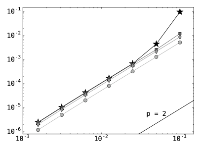
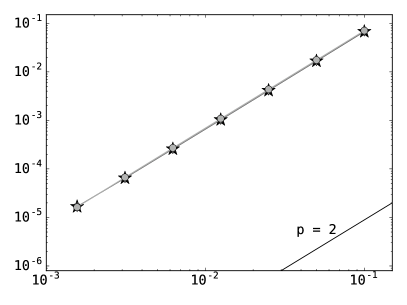
Figure 1. Computed error norms $\|{\boldsymbol{u}}_{h}^{\rm ref}-{\boldsymbol{u}}_{h}\|_{{\boldsymbol{H}}^{1}}$ (left) and $\|q_{h}^{\rm ref}-q_{h}\|_{(H^{1})^{\prime}}$ (right), for varying time-step $k$, with $k^{\rm ref}=0.1\cdot 2^{-8}$, and fixed mesh size. Results for mesh sizes $h=2^{-3}$ ($\ocircle$), $h=2^{-4}$ ($\lozenge$), $h=2^{-5}$ ($\square$) and $h=2^{-6}$ ($\bigstar$). Notice that, since $q_{h}$ is naturally computed at half time steps, the corresponding errors are computed at $t=1-k/2$ for each time-step $k$.

Figure 1 shows the results for $\|{\boldsymbol{u}}-{\boldsymbol{u}}_{h}\|_{{\boldsymbol{H}}^{1}}$ and $\|q-q_{h}\|_{(H^{1})^{\prime}}$. A comparison of this figure with the values reported in Tables 1 and 2 confirms that the time discretization error is smaller than the space discretization one. Second order convergence is also apparent estimating the convergence rate as $\log_{2}\rho$, where (see [36, Eq (4.7)])

$$\rho=\frac{\|{\boldsymbol{u}}_{h}^{k}-{\boldsymbol{u}}_{h}^{k/2}\|_{{\boldsymbol{H}}^{1}}}{\|{\boldsymbol{u}}_{h}^{k/2}-{\boldsymbol{u}}_{h}^{k/4}\|_{{\boldsymbol{H}}^{1}}},$$

as shown in Table 3.

Table 3. Estimated time discretization errors $\|{\boldsymbol{u}}_{h}^{k}-{\boldsymbol{u}}_{h}^{k/2}\|_{H^{1}}$ for $k=0.1\cdot 2^{-j}$, $j=0,\dots,5$, for four triangular grids with $h=2^{-i}$, $i=3,4,5,6$ (see also Figure 1). The resulting convergence rates are also reported.

$j$	$h=2^{-3}$		$h=2^{-4}$		$h=2^{-5}$		$h=2^{-6}$
0	$3.9\cdot 10^{-3}$	–	$6.6\cdot 10^{-3}$	–	$9.9\cdot 10^{-3}$	–	$9.2\cdot 10^{-2}$	–
1	$9.7\cdot 10^{-4}$	1.9989	$1.6\cdot 10^{-3}$	2.0018	$2.0\cdot 10^{-3}$	2.3348	$4.1\cdot 10^{-3}$	4.5030
2	$2.4\cdot 10^{-4}$	1.9998	$4.1\cdot 10^{-4}$	2.0004	$4.9\cdot 10^{-4}$	2.0004	$5.1\cdot 10^{-4}$	3.0037
3	$6.1\cdot 10^{-5}$	1.9999	$1.0\cdot 10^{-4}$	2.0001	$1.2\cdot 10^{-4}$	2.0001	$1.3\cdot 10^{-4}$	2.0001
4	$1.5\cdot 10^{-5}$	2.0000	$2.6\cdot 10^{-5}$	2.0000	$3.1\cdot 10^{-5}$	2.0000	$3.2\cdot 10^{-5}$	2.0000
5	$3.8\cdot 10^{-6}$	2.0000	$6.4\cdot 10^{-6}$	2.0000	$7.7\cdot 10^{-6}$	2.0000	$7.9\cdot 10^{-6}$	2.0000

7.2. Behaviour for singular solutions

After considering the behaviour of the scheme for problems with smooth solutions, we turn our attention to problems including singularities. In fact, singularities of the form ${\boldsymbol{u}}\sim\frac{{\boldsymbol{x}}-{\boldsymbol{x}}_{0}}{|{\boldsymbol{x}}-{\boldsymbol{x}}_{0}|}$ are very important in the study of liquid crystals, and various related test cases have been considered in the literature [34, 18, 35, 11, 6, 26, 15].

An important distinction here must be done between two- and three-dimensional problems, since such singularities have a finite energy in the three-dimensional case but not in the two-dimensional one (mathematically, they belong to ${\boldsymbol{H}}^{1}(\Omega)$ for $\Omega\subset\mathds{R}^{3}$ but not for $\Omega\subset\mathds{R}^{2}$). From a practical perspective, a singular solution can be approximated in the chosen finite element space both in two and three spatial dimensions, for instance by nodal interpolation (provided that none of the nodes coincides with the singular point ${\boldsymbol{x}}_{0}$); the resulting function belongs to ${\boldsymbol{H}}^{1}$ and can serve as an initial condition for a time dependent computation. Hence, one might be tempted to dismiss the distinction between the two cases as a merely theoretical argument with no practical implications. However, this would be incorrect, as the following results demonstrate. Indeed, for three-dimensional problems, the theoretical analysis provided above holds, and our method is guaranteed to satisfy our stability estimates when the grid is refined. For the two-dimensional case, on the contrary, the theoretical analysis does not apply and nothing can be said a priori; nevertheless, computational experiments indicate that, although it is possible to compute a numerical solution, such a solution critically depends on the numerical discretization, does not converge to a well defined limit when the grid is refined and is thus essentially meaningless.

Before discussing the numerical results, it is useful to provide a qualitative analysis of the problem of representing a singular solution with a finite element function. In two spatial dimensions, for a structured, triangular grid, the finite element function will resemble the patterns shown in Figure 2. This implies that

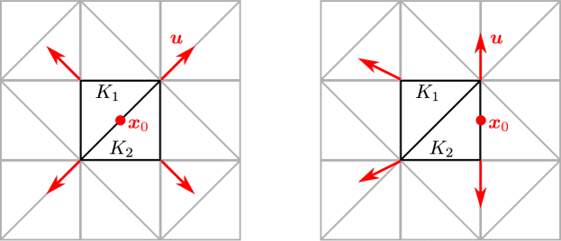
Figure 2. Interpolation of a singular solution of the form $\frac{{\boldsymbol{x}}-{\boldsymbol{x}}_{0}}{|{\boldsymbol{x}}-{\boldsymbol{x}}_{0}|}$ on a structured, triangular grid for different location of ${\boldsymbol{x}}_{0}$ with respect to the computational grid.

there are at least two elements where the numerical solution has $\mathcal{O}(1)$ variations within an $\mathcal{O}(h)$ distance, which, in turn, implies that the energy of the discrete solution $\|\nabla{\boldsymbol{u}}_{h}\|_{\boldsymbol{L}^{2}}^{2}$ undergoes $\mathcal{O}(1)$ variations for an $\mathcal{O}(h)$ displacement of the singularity. For instance, referring to Figure 2, and given that we consider linear finite elements, it easy to check that the two elements containing the singularity, $K_{1}$ and $K_{2}$, contribute to the total energy with $\|\nabla{\boldsymbol{u}}_{h}\|_{\boldsymbol{L}^{2}(K_{1}\cup K_{2})}^{2}=4$ and $\|\nabla{\boldsymbol{u}}_{h}\|_{\boldsymbol{L}^{2}(K_{1}\cup K_{2})}^{2}=(22-2\sqrt{5})/5$ for the two depicted configurations, independently of $h$. Since the solution is smooth far from the singularity, such $\mathcal{O}(1)$ energy variations for $\mathcal{O}(h)$ displacements of the singularity are also present if we consider the total energy $\|\nabla{\boldsymbol{u}}_{h}\|$; this is shown in Figure 3 (left)

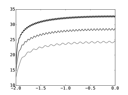
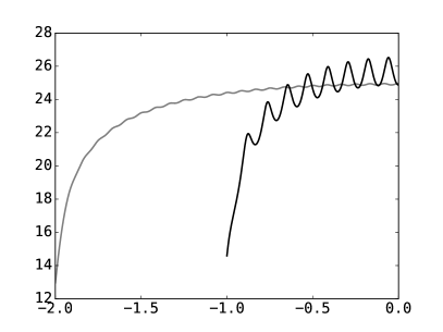
Figure 3. Energy $\|\nabla{\boldsymbol{u}}_{h}\|^{2}$, for $\Omega=(-2,2)\times(-1,1)$ and ${\boldsymbol{u}}_{h}$ defined as the nodal interpolant of $\frac{{\boldsymbol{x}}-{\boldsymbol{x}}_{0}}{|{\boldsymbol{x}}-{\boldsymbol{x}}_{0}|}$ on a structured, triangular mesh, as a function of ${\boldsymbol{x}}_{0}$. Left: values for three isotropic grids with $34\times 17$ elements (light gray), $66\times 33$ elements (gray) and $130\times 65$ elements (black) as functions of $x_{0}$ such that ${\boldsymbol{x}}_{0}=(x_{0},0)^{T}$, $x_{0}\in[-2,0]$. Right: values for a single anisotropic grid with $48\times 17$ elements and ${\boldsymbol{x}}_{0}=(x_{0},0)^{T}$ (gray) and ${\boldsymbol{x}}_{0}=(1/24\,,y_{0})^{T}$ (black), with $x_{0}\in[-2,0]$ and $y_{0}\in[-1,0]$. The large-scale variations are due to the fact that, as ${\boldsymbol{x}}_{0}$ approaches the boundary of the domain, a “large part” of the field lies outside $\Omega$.

where we plot, for various mesh sizes, the total energy of the nodal interpolant of $\frac{{\boldsymbol{x}}-{\boldsymbol{x}}_{0}}{|{\boldsymbol{x}}-{\boldsymbol{x}}_{0}|}$ on $\Omega=(-2,2)\times(-1,1)$ as a function of the position of ${\boldsymbol{x}}_{0}$, specified as ${\boldsymbol{x}}_{0}=(x_{0},0)^{T}$ for $x_{0}\in[-2,0]$. Since the energy can not increase during the time evolution because of (4), the result of this grid dependence of the energy itself can be seen as a “potential barrier” which tends to trap the singularity between the grid vertexes, in Figure 2 (left). Two important characteristics of such a barrier can be noted. First of all, it is independent of $h$, so that refining the grid has no effect on it; this can be seen both by noting that, for elements such as $K_{1}$ and $K_{2}$ in Figure 2, $\|\nabla{\boldsymbol{u}}_{h}\|^{2}\sim h^{-2}$ and the area element is proportional to $h^{2}$, as well as by considering Figure 3 (left) where the amplitude of the small-scale oscillations is constant for different resolutions. The second characteristic of the potential barrier is its dependency on the grid anisotropy. This is illustrated in Figure 4, which shows how, for a uniform, triangular grid with different spacings in the two Cartesian directions, the variation of the finite element solution is more pronounced when the singularity moves from ${\boldsymbol{x}}_{0}$ to ${\boldsymbol{x}}_{0}^{\prime}$ compared to a displacement from ${\boldsymbol{x}}_{0}$ to ${\boldsymbol{x}}_{0}^{\prime\prime}$.

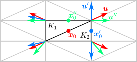
Figure 4. Interpolation of a singular solution of the form $\frac{{\boldsymbol{x}}-{\boldsymbol{x}}_{0}}{|{\boldsymbol{x}}-{\boldsymbol{x}}_{0}|}$ on a structured, triangular grid for different location of ${\boldsymbol{x}}_{0}$ with respect to the computational grid. Contrary to the case shown in Figure 2, we consider here an anisotropic grid, with different spacings in the two Cartesian directions.

Again, this qualitative description is confirmed considering a specific example of a grid composed of $48\times 17$ elements for $\Omega=(-2,2)\times(-1,1)$ and evaluating the energy of the finite element solution when the singularity is displaced along the two Cartesian axes, as shown in Figure 3(right) where it is apparent that the amplitude of the grid-inducedoscillations is much larger when the singularity is displaced along the direction with the largest grid spacing.

For three spatial dimensions, this qualitative analysis still holds, up to one important difference: in such a case, $\mathcal{O}(1)$ variations over an $\mathcal{O}(h)$ distance result in $\mathcal{O}(h)$ energy contributions, because now it is still $\|\nabla{\boldsymbol{u}}_{h}\|^{2}\sim h^{-2}$ but the area element is proportional to $h^{3}$. Hence, for three-dimensional computations, the discrete potential barriers at the element boundaries vanish when the grid is refined.

Summarizing now the conclusions of the qualitative analysis, we can expect that, initializing the finite element computation interpolating a singular field ${\boldsymbol{u}}$, the numerical solution will be strongly influenced by the computational grid. Moreover, while three-dimensional computation will converge to the analytic solution, two-dimensional ones will not show any consistent limit when the grid is refined. Indeed, this is precisely the outcome of our numerical experiments, which we now describe in the remaining of the present section.

The initial condition for the numerical experiments is a modified version of the one considered in [35] and is defined as

$${\boldsymbol{u}}_{0}({\boldsymbol{x}})=\frac{\tilde{{\boldsymbol{u}}}_{0}({\boldsymbol{x}})}{|\tilde{{\boldsymbol{u}}}_{0}({\boldsymbol{x}})|},\qquad\tilde{{\boldsymbol{u}}}_{0}({\boldsymbol{x}})=w({\boldsymbol{x}})\,({\boldsymbol{x}}+{\boldsymbol{\delta}})+(1-w({\boldsymbol{x}}))(-({\boldsymbol{x}}-{\boldsymbol{\delta}}))$$

with

$$w({\boldsymbol{x}})=\frac{1}{1+\exp(5x)}$$

and ${\boldsymbol{x}}=(x,y)^{T}$, ${\boldsymbol{\delta}}=(\delta,0)^{T}$ and and ${\boldsymbol{x}}=(x,y,z)^{T}$, ${\boldsymbol{\delta}}=(\delta,0,0)^{T}$ in two and three space dimensions, respectively. This corresponds to two singularities located on the $x$ axis approximately at $x=\pm\delta$ having opposite sign and thus repelling each other. We take $\gamma=1$ and $\alpha=0$, while the computational domain is $\Omega=(-2,2)\times(-1,1)$ in two dimensions and $\Omega=(-2,2)\times(-1,1)\times(-1,1)$ in three dimensions. The computational grid is uniform and structured and is obtained, in two spatial dimensions, partitioning $\Omega$ into rectangles with dimensions $\Delta_{x},\Delta_{y}$ and dividing each rectangle into two triangles with alternating direction, obtaining a grid analogous to those depicted in Figures 2 and 4. For the three dimensional case, the construction is similar witch each prism being divided into six tetrahedral elements. Grids will be defined also by means of the number of subdivisions in each Cartesian direction, so that a grid with $N_{x}\times N_{y}$ elements correspond to $\Delta_{x}=4/N_{x},\Delta_{y}=2/N_{y}$. The overall evolution of the numerical solution is determined by the interplay between the large-scale and the grid-scale energy variations associated with a displacement of the two singularities: the former corresponds to an energy decrease when the two singularities drift apart, the latter has been analyzed previously in this section and tends to lock the singularities between the grid vertexes. The initial separation is chosen so that, for all the considered computations, a transient is observed at least in the initial phase, with the large-scale effect overcoming the grid one. In practice, we take $\delta=0.0625$ in two dimensions and $\delta=0.5$ in three dimensions and choose in both cases adequate grid anisotropy levels.

The time evolution of the energy of the finite element solution for the two dimensional case in shown in Figure 5 for four levels of grid anisotropy and two levels of grid refinement.

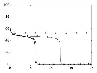
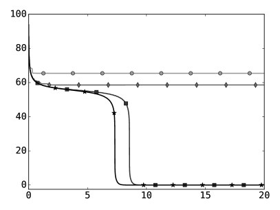
Figure 5. Time evolution of $\|\nabla{\boldsymbol{u}}_{h}\|^{2}$ for two repelling singularities in two space dimensions for different levels of grid anisotropy, defined as $\Delta_{y}:\Delta_{x}$, namely $1:1$ ($\ocircle$), $6:5$ ($\lozenge$), $7:5$ ($\square$) and $8:5$ ($\bigstar$). Left: grids with $34\times 17$, $41\times 17$, $48\times 17$ and $54\times 17$ elements. Right: grids with $66\times 33$, $79\times 33$, $92\times 33$ and $106\times 33$ elements.

The energy decreases as the two singularities drift apart and drops to zero if they reach the boundary and leave the computational domain. The first observation is that, depending on the anisotropy of the grid, the two singularities can reach the boundary (when the anisotropy is such that the potential barrier associated with the grid for displeacemet along $x$ is small) or reach a steady state condition inside the grid after an initial transient. The second observation is that the drift velocity is strongly affected by the grid anisotropy. A third observation is that the energy time evolution has a step pattern where each step corresponds to the displacement of the singularities over one grid element, i.e. to the crossing of one potential barrier. A fourth observation is that, when the grid is refined, the effect of the grid is not reduced: in fact, for finer grids, the spread among the computations with similar resolution but different stretching increases and the numerical steady state is reached earlier. Finally, we mention that that analogous computations using unstructured grids, not reported here, show that even the direction in which the singularities drift is strongly affected by the computational grid.

Repeating now the experiment in three spatial dimensions, we obtain the results reported in Figure 6. The step pattern observed for two-dimensional computations is still present, however we notice that: a) regardless of the grid anisotropy, the singularities leave the computational domain; b) refining the grid, the amplitute of the steps decreases and a tendency of the solutions obtained for different levels of grid anisotropy to converge to a unique limit can be observed.

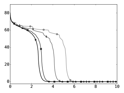
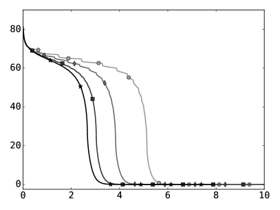
Figure 6. Time evolution of $\|\nabla{\boldsymbol{u}}_{h}\|^{2}$ for two repelling singularities in three space dimensions for different levels of grid anisotropy, which can be defined as $\Delta_{y}:\Delta_{x}$ thanks to the fact that $\Delta_{y}=\Delta_{z}$, namely: $10:17$ ($\ocircle$), $10:15$ ($\lozenge$), $10:12$ ($\square$) and $1:1$ ($\bigstar$). Left: grids with $20\times 17\times 17$, $23\times 17\times 17$, $28\times 17\times 17$ and $34\times 17\times 17$ elements. Right: grids with $38\times 33\times 33$, $44\times 33\times 33$, $53\times 33\times 33$ and $66\times 33\times 33$ elements.

8. Conclusion

In this paper we have proposed and analyzed a unified saddle-point stable finite element method for approximating the harmonic map heat and Landau–Lifshitz–Gilbert equation. We have mainly proved that the numerical solution satisfies an energy law and a nodal satisfaction of the unit sphere, and the associated Lagrange multiplier satisfies an inf-sup condition. The key ingredients are using piecewise linear finite element spaces, applying a nodal interpolation to the terms involving the nonlinear restriction and a mass lumping technique to the terms involving time derivatives.

This work has important implications in the context of the Ericksen–Leslie equations which incorporate a convective term to the harmonic map heat equation. While other existing approaches in the literature are not readily adapted to these equations due to the convective term, our proposed method may be directly applied to them without any modification keeping the desired properties above mentioned.

Concerning the numerical results we have shown that the finite element solution computed by a nonlinear Crank–Nicolson method, which is solved by using semi-implicit Euler iterations, enjoys the expected accurate approximations. Moreover, we have identified that the dynamics of singularity points depends on dimension. That is, we have seen that, depending on the mesh anisotropy, in two dimensions, two singularity points can either be trapped among two elements of the mesh or move according to their sign. Instead, in three dimensions, the trapping effect does not occur. Therefore, some care must be taken in simulating singularities in two dimensions since these do not have finite energy and the limit equation only holds in the sense of measures.

References

- [1] F. Alouges, A new finite element scheme for Landau–Lifchitz equations, Discrete Contin. Dyn. Syst. Ser. S 1 (2008), no. 2, 187–196.
- [2] F. Alouges, P. Jaisson, Convergence of a finite element discretization for the Landau–Lifshitz equations in micromagnetism, Math. Models Methods Appl. Sci. 16 (2006), no. 2, 299–316.
- [3] F. Alouges, E. Kritsikis, J.-C. Toussaint, A convergent finite element approximation for the Landau–Lifschitz–Gilbert equation, Physica B 407 (2012). 1345–1349.
- [4] F. Alouges, E. Kritsikis, J. Steiner, J.-C. Toussaint, A convergent and precise finite element scheme for Landau–Lifschitz-Gilbert equation, Numer. Math. 128 (2014), no. 3, 407–430.
- [5] S. Badia, F. Guillén-González, J.V. Gutiérrez-Santacreu, An overview on numerical analyses of nematic liquid crystal flows, Arch. Comput. Methods Eng. 18 (2011), no. 3, 285–313.
- [6] S. Badia, F. Guillén-González, J. V. Gutiérrez-Santacreu, Finite element approximation of nematic liquid crystal flows using a saddle-point structure, J. Comput. Phys. 230 (2011), no. 4, 1686–1706.
- [7] S. Bartels, Stability and convergence of finite-element approximation schemes for harmonic maps, SIAM J. Numer. Anal. 43 (2005), no. 1, 220-238.
- [8] S. Bartels, A. Prohl, Convergence of an implicit finite element method for the Landau–Lifshitz–Gilbert equation, SIAM J. Numer. Anal. 44, pp. 1405–1419 (2006).
- [9] S. Bartels, A. Prohl, Constraint preserving implicit finite element discretization of harmonic map flow into spheres, Math. Comp. 76, pp. 1847–1859 (2007).
- [10] S. Bartels, C. Lubich, A. Prohl, Convergent discretization of heat and wave map flows to spheres using approximate discrete Lagrange multipliers, Math. Comp. 78 (2009), no. 267, 1269–1292.
- [11] R. Becker, X. Feng, and A. Prohl, Finite element approximations of the Ericksen–Leslie model for nematic liquid crystal flow, SIAM J. Numer. Anal., 46 (2008), pp. 1704–1731.
- [12] F. Brezzi, M. Fortin, Mixed and hybrid finite element methods, Springer Series in Computational Mathematics, 15. Springer-Verlag, New York, 1991.
- [13] S. C. Brenner, L. R. Scott, The mathematical theory of finite element methods, Third edition. Texts in Applied Mathematics, 15. Springer, New York, 2008.
- [14] J. Jr. Douglas, T. Dupont, L. Wahlbin, The stability in of the -projection into finite element function spaces, Numer. Math. 23 (1975), 193–197.
- [15] R. C. Cabrales, F. Guillén-González, J. V. Gutiérrez-Santacreu, A time-splitting finite-element stable approximation for the Ericksen-Leslie equations, SIAM J. Sci. Comput. 37 (2015), no. 2, B261–B282.
- [16] I. Cimrák, Error estimates for a semi-implicit numerical scheme solving the Landau–Lifshitz equation with an exchange field, IMA J. Numer. Anal. 25 (2005), no. 3, 611–634.
- [17] I. Cimrák, A survey on the numerics and computations for the Landau–Lifshitz equation of micromagnetism, Arch. Comput. Methods Eng. 15 (2008), no. 3, 277–309.
- [18] Q. Du, B. Guo, J. Shen, Fourier spectral approximation to a dissipative system modeling the flow of liquid crystals, SIAM J. Numer. Anal. 39 (2000), no. 3, 735–762.
- [19] H. C. Elman, G. H. Golub, Inexact and preconditioned Uzawa algorithms for saddle point problems, SIAM J. Numer. Anal. 31 (6) (1994) 1645–1661.
- [20] J. Ericksen, Conservation laws for liquid crystals, Trans. Soc. Rheology, 5 (1961), 22–34.
- [21] J. Ericksen, Continuum theory of nematic liquid crystals, Res. Mechanica, 21 (1987), 381–392.
- [22] A. Ern, J.-L. Guermond, Theory and practice of finite elements, Applied Mathematical Sciences, 159. Springer-Verlag, New York, 2004.
- [23] T. L. Gilbert, A Lagrangian formulation of the gyromagnetic equation of the magnetization fields, Phys. Rev. 100 (1955), 1243.
- [24] T.L. Gilbert, A phenomenological theory of damping in ferromagnetic materials, IEEE Trans. Magn. 40 (2004), 3443–3449.
- [25] F. Guillén-González, J. V. Gutiérrez-Santacreu, A linear mixed finite element scheme for a nematic Ericksen–Leslie liquid crystal model, ESAIM Math. Model. Numer. Anal., 47 (2013), pp. 1433–1464.
- [26] F. Guillén-Gonzalez, J. Koko, A splitting in time scheme and augmented Lagrangian method for a nematic liquid crystal problem, J. Sci. Comput., 65 (2015), pp. 1129–1144.
- [27] Q. Hu, X.-C. Tai, R. Winther, A saddle point approach to the computation of harmonic maps, SIAM J. Numer. Anal. 47 (2009), no. 2, 1500–1523.
- [28] C. Johnson, A. Szepessy, P. Hansbo, On the convergence of shock-capturing streamline diffusion finite element methods for hyperbolic conservation laws. Mathematics of Computation, 54 (1990), pp. 107–129.
- [29] E. Kritsikis, A. Vaysset, L. D. Buda-Prejbeanu, F. Alouges, J.-C. Toussaint, Beyond first-order finite element schemes in micromagnetics. J. Comput. Phys. 256 (2014), 357–366.
- [30] M. Kruzik, A. Prohl. Recent developments in the modeling, analysis, and numerics of ferromagnetism. SIAM Rev. 48 (2006), no. 3, 439–483.
- [31] L. D. Landau, E. M. Lifshitz, Theory of the dispersion of magnetic permeability in ferromagnetic bodies, Phys. Z. Sowietunion, 8 (1935), 153.
- [32] F. Leslie, Some constitutive equations for liquid crystals, Arch. Rational Mech. Anal., 28 (1968), 265–283.
- [33] F. Leslie, Theory of flow phenomena in liquid crystals, in Advances in Liquid Crystals, Vol. 4, G. H. Brown, ed., Academic Press, New York, 1979,1–81.
- [34] C. Liu, N. J. Walkington, Approximation of liquid crystal flows, SIAM J. Numer. Anal. 37 (2000), no. 3, 725–741.
- [35] C. Liu, N. J. Walkington, Mixed methods for the approximation of liquid crystal flows, ESAIM Math. Model. Numer. Anal., 36 (2002), pp. 205–222.
- [36] M. Mu, X. Zhu, Decoupled schemes for a non-stationary mixed Stokes–Darcy model, Math. Comp. 79, pp. 707–731 (2010).
- [37] A. Prohl, Computational micromagnetism, Advances in Numerical Mathematics. B. G. Teubner, Stuttgart, 2001.