Soliton-like behavior in fast two-pulse collisions in weakly perturbed linear physical systems

Abstract

We demonstrate that pulses of linear physical systems, weakly perturbed by nonlinear dissipation, exhibit soliton-like behavior in fast collisions. The behavior is demonstrated for linear waveguides with weak cubic loss and for systems described by linear diffusion-advection models with weak quadratic loss. We show that in both systems, the expressions for the collision-induced amplitude shifts due to the nonlinear loss have the same form as the expression for the amplitude shift in a fast collision between two optical solitons in the presence of weak cubic loss. Our analytic predictions are confirmed by numerical simulations with the corresponding coupled linear evolution models with weak nonlinear loss. These results open the way for studying dynamics of fast collisions between pulses of weakly perturbed linear physical systems in an arbitrary spatial dimension.

I Introduction

Solitons, which are stable shape preserving traveling-wave solutions of nonlinear wave models, appear in a wide range of fields, including hydrodynamics Zakharov84 , condensed matter physics Malomed89 , optics Agrawal2001 ; Mollenauer2006 , and plasma physics Horton96 . The robustness of solitons in soliton collisions, i.e., the fact that the solitons do not change their shape in the collisions, is one of their most fundamental properties Zakharov84 ; Malomed89 ; Agrawal2001 . This property is often associated with the integrable nature of the corresponding nonlinear wave models Zakharov84 .

Another major property of solitons is manifested during fast inter-soliton collisions, i.e., during collisions for which the difference between the central frequencies (and group velocities) of the solitons is much larger than the soliton spectral width. This important property concerns the simple scaling relations satisfied by the soliton parameters, such as position, phase, amplitude, and frequency during fast collisions. It holds both in the absence of perturbations and in the presence of weak perturbations to the integrable nonlinear wave model. For example, the phase and position of fundamental solitons of the nonlinear Schrödinger (NLS) equation exhibit a shift during a two-soliton collision Zakharov84 . For fast collisions, the collision-induced phase and position shifts of soliton 1, for example, scale as $\eta_{2}/|\Delta\beta|$ and $-\eta_{2}/\Delta\beta^{2}$, where $\eta_{j}$ with $j=1,2$ are the soliton amplitudes, $\Delta\beta=\beta_{2}-\beta_{1}$, and $\beta_{j}$ with $j=1,2$ are the soliton frequencies Zakharov84 ; MM98 ; CP2005 . Furthermore, during fast collisions in the presence of weak cubic loss, solitons of the NLS equation experience amplitude and frequency shifts that scale as $-\epsilon_{3}\eta_{1}\eta_{2}/|\Delta\beta|$ and $-\epsilon_{3}\eta_{1}^{2}\eta_{2}/\Delta\beta^{2}$ for soliton 1, where $\epsilon_{3}$ is the cubic loss coefficient PNC2010 . Similar simple scaling relations hold for fast two-pulse collisions of NLS solitons in the presence of other weak perturbations, such as delayed Raman response Chi89 ; Malomed91 ; Kumar98 ; CP2005 ; P2004 ; NP2010 , and higher-order nonlinear loss PC2012 .

The simple scaling relations of collision-induced changes in soliton parameters are often associated with the shape preserving and stability properties of the solitons PNC2010 ; CP2005 ; PC2012 . Since the latter two properties are related with the integrability of the nonlinear wave model, one might also relate the simple scaling behavior in fast two-soliton collisions to the integrability of the model. In contrast, one expects very different behavior in collisions between pulses that are not shape preserving, since changes in pulse shape or instability might lead to the breakdown of the simple dynamics observed in fast two-soliton collisions. The latter expectation should certainly hold in linear physical systems that are weakly perturbed by nonlinear dissipation, since the pulses of the linear systems are in general not shape preserving Tkach97 ; Agrawal2001 ; Agrawal89a . For this reason, it is often claimed that conclusions drawn from analysis of soliton collisions cannot be applied to collisions between pulses of weakly perturbed linear systems Agrawal2001 ; Mollenauer2006 ; Tkach97 ; Agrawal89b ; PNC2010 ; PCG2003 ; PCG2004 .

In the current paper, we show that the point of view of fast collisions between pulses that are not shape preserving, described above, is erroneous. More specifically, we demonstrate that pulses of linear physical systems, weakly perturbed by nonlinear dissipation, exhibit simple soliton-like scaling behavior. The behavior is demonstrated for two major examples: (a) linear waveguide systems with weak cubic loss; (b) systems described by linear diffusion-advection models with weak quadratic loss. For both systems, we show that the expressions for the collision-induced amplitude shifts due to the nonlinear loss have the same form as the expression for the amplitude shift in a fast collision between two optical solitons in the presence of weak cubic loss. We validate our analytic predictions by numerical simulations with the corresponding perturbed coupled linear evolution models. Our results open the way for studying dynamics of fast collisions between pulses of weakly perturbed linear physical systems in an arbitrary spatial dimension, which is typically impossible for collisions between solitons in systems described by NLS models due to the instability of the solitons in dimension higher than one Zakharov84 .

The calculation of the collision-induced amplitude shift in the current paper is based on a generalization of the the perturbation technique, developed in Refs. PCG2003 ; PCG2004 for calculating the effects of weak perturbations on fast collisions between NLS solitons. This perturbation technique was first used to calculate the effects of weak conservative perturbations, such as third-order dispersion PCG2003 ; PCG2004 and quintic nonlinearity SP2004 on fast two-soliton collisions. Later on it was shown that the perturbation technique can also be used for calculating the effects of weak dissipative perturbations on fast soliton collisions CP2005 ; PNC2010 ; PC2012 ; P2004 . In the current paper we further generalize and extend the perturbation technique to allow treatment of fast two-pulse collisions in linear physical systems, weakly perturbed by nonlinear dissipation. The main assumption of the generalized perturbation technique is that the smallest relevant length scale (or time scale) in the problem is the collision length (or collision time interval), which is the distance (or time interval) along which the two colliding pulses overlap. This assumption along with the assumptions of a fast collision and weak dissipation allow us to obtain simple scaling relations for the collision-induced amplitude shifts, which are similar in form to the simple scaling relations obtained for fast collisions between two optical solitons in the presence of weak cubic loss.

The rest of the paper is organized as follows. In section II, we obtain the analytic prediction for the collision-induced amplitude shift in a fast collision between two optical pulses in a linear waveguide with weak linear and cubic loss. We then compare the analytic prediction with results of numerical simulations of the collision with the perturbed coupled linear propagation model. In section III, we obtain the analytic prediction for the collision-induced amplitude shift in a fast collision between two concentration pulses in systems described by perturbed coupled linear diffusion-advection models with weak linear and quadratic loss. In addition, we present a comparison of the analytic prediction with the results of numerical simulations with the perturbed coupled linear diffusion-advection model. In section IV, we present our conclusions. In Appendix A, we derive the relations between the collision-induced amplitude shift and the collision-induced change in pulse shape. Appendix B is devoted to a description of the procedures used for calculating the values of the collision-induced amplitude shift from the analytic predictions and from results of numerical simulations.

II Fast collisions in linear waveguides

II.1 Propagation model

We consider fast collisions between two optical pulses in linear waveguides with weak linear and cubic loss. The dynamics of the collision is described by the following system of perturbed coupled linear propagation equations Agrawal2001 ; Agrawal2007a ; PNC2010 :

$$\!\!\!\!\!\!\!i\partial_{z}\psi_{1}\!-\!\mbox{sgn}(\tilde{\beta}_{2})\partial_{t}^{2}\psi_{1}\!=\!-i\epsilon_{1}\psi_{1}\!-\!i\epsilon_{3}|\psi_{1}|^{2}\psi_{1}\!-\!2i\epsilon_{3}|\psi_{2}|^{2}\psi_{1},$$

$$\!\!\!\!\!\!\!i\partial_{z}\psi_{2}+id_{1}\partial_{t}\psi_{2}-\mbox{sgn}(\tilde{\beta}_{2})\partial_{t}^{2}\psi_{2}=-i\epsilon_{1}\psi_{2}-i\epsilon_{3}|\psi_{2}|^{2}\psi_{2}$$

$$-2i\epsilon_{3}|\psi_{1}|^{2}\psi_{2},\!\!\!\!\!\!\!\!$$ (1)

where $\psi_{1}$ and $\psi_{2}$ are the envelopes of the electric fields of the pulses, $z$ is propagation distance, and $t$ is time Dimensions1 . In Eq. (1), $d_{1}$ is the group velocity coefficient, $\tilde{\beta}_{2}$ is the second-order dispersion coefficient, and $\epsilon_{1}$ and $\epsilon_{3}$ are the linear and cubic loss coefficients, which satisfy $0<\epsilon_{1}\ll 1$ and $0<\epsilon_{3}\ll 1$. The terms $-\mbox{sgn}(\tilde{\beta}_{2})\partial_{t}^{2}\psi_{j}$ on the left hand side of Eq. (1) are due to second-order dispersion, while $id_{1}\partial_{t}\psi_{2}$ is associated with the group velocity difference. The first terms on the right hand side of Eq. (1) describe linear loss effects, while the second and third terms describe intra-pulse and inter-pulse effects due to cubic loss.

II.2 Calculation of the amplitude shift in a fast two-pulse collision

We consider a fast collision between two pulses with generic shapes and with tails that exhibit exponential or faster than exponential decay. We assume that the pulses can be characterized by initial amplitudes $A_{j}(0)$, initial widths $W_{j0}$, initial positions $y_{j0}$, and initial phases $\alpha_{j0}$. Thus, for a collision between two Gaussian pulses, for example, the initial envelopes of the electric fields are:

$$\!\!\!\!\!\!\!\psi_{j}(t,0)=A_{j}(0)\exp[-(t-y_{j0})^{2}/(2W_{j0}^{2})+i\alpha_{j0}],\!\!\!\!\!\!\!\!$$ (2)

where $j=1,2$. As another example, for a collision between two square pulses, the initial envelopes of the electric fields are:

$$\!\!\!\!\!\!\!\!\!\psi_{j}(t,0)=\left\{\begin{array}[]{l l}A_{j}(0)\exp(i\alpha_{j0})&\;\;\mbox{for}\;\;|t-y_{j0}|\leq W_{j0}/2,\\ 0&\;\;\mbox{for}\;\;|t-y_{j0}|>W_{j0}/2,\\ \end{array}\right.$$ (5)

where $j=1,2$. We assume a complete collision, such that the two pulses are well separated at $z=0$ and at the final distance $z=z_{f}$.

Let us discuss the implications of the assumption of a fast collision. For this purpose, we define the collision length $\Delta z_{c}$, which is the distance along which the envelopes of the colliding pulses overlap, by $\Delta z_{c}=W_{0}/|d_{1}|$, where for simplicity we assume $W_{10}=W_{20}=W_{0}$. The assumption of a fast collision means that $\Delta z_{c}$ is the shortest length scale in the problem. In particular, $\Delta z_{c}\ll z_{D}$, where $z_{D}=W_{0}^{2}/2$ is the dispersion length. Using the definitions of $\Delta z_{c}$ and $z_{D}$, we obtain $W_{0}|d_{1}|/2\gg 1$, as the condition for a fast collision.

Our perturbative calculation of the amplitude shift in a fast collision is a generalization of the perturbative technique, developed in Refs. PCG2003 ; PCG2004 for calculating the effects of weak perturbations on fast two-soliton collisions. In an analogy with the fast two-soliton collision case, we look for a solution of Eq. (1) in the form

$$\!\!\!\!\!\!\!\psi_{j}(t,z)=\psi_{j0}(t,z)+\phi_{j}(t,z),$$ (6)

where $j=1,2$, $\psi_{j0}$ are the solutions of Eq. (1) without the inter-pulse interaction terms, and $\phi_{j}$ describe corrections to $\psi_{j0}$ due to inter-pulse interaction. By definition, $\psi_{10}$ and $\psi_{20}$ satisfy

$$\!\!\!\!\!\!\!i\partial_{z}\psi_{10}\!-\!\mbox{sgn}(\tilde{\beta}_{2})\partial_{t}^{2}\psi_{10}\!=\!-i\epsilon_{1}\psi_{10}\!-\!i\epsilon_{3}|\psi_{10}|^{2}\psi_{10},\!\!\!\!\!\!\!\!$$ (7)

and

$$\!\!\!\!\!\!\!i\partial_{z}\psi_{20}+id_{1}\partial_{t}\psi_{20}-\mbox{sgn}(\tilde{\beta}_{2})\partial_{t}^{2}\psi_{20}=$$

$$-i\epsilon_{1}\psi_{20}-i\epsilon_{3}|\psi_{20}|^{2}\psi_{20}.$$ (8)

We now substitute relation (6) into Eq. (1) and use Eqs. (7) and (8) to obtain equations for the $\phi_{j}$. We concentrate on the calculation of $\phi_{1}$, since the calculation of $\phi_{2}$ is similar. Taking into account only leading-order effects of the collision, we can neglect terms containing $\phi_{j}$ on the right hand side of the resulting equation. We therefore obtain:

$$i\partial_{z}\phi_{1}-\mbox{sgn}(\tilde{\beta}_{2})\partial_{t}^{2}\phi_{1}=-2i\epsilon_{3}|\psi_{20}|^{2}\psi_{10}.$$ (9)

Continuing the analogy with the fast two-soliton collision, we substitute $\psi_{j0}(t,z)=\Psi_{j0}(t,z)\exp[i\chi_{j0}(t,z)]$ and $\phi_{1}(t,z)=\Phi_{1}(t,z)\exp[i\chi_{10}(t,z)]$, where $\Psi_{j0}$ and $\chi_{j0}$ are real-valued, into Eq. (9). This substitution yields the following equation for $\Phi_{1}$:

$$i\partial_{z}\Phi_{1}-\left(\partial_{z}\chi_{10}\right)\Phi_{1}-\mbox{sgn}(\tilde{\beta}_{2})\left[\partial_{t}^{2}\Phi_{1}+2i\left(\partial_{t}\chi_{10}\right)\partial_{t}\Phi_{1}\right.$$

$$\left.+i\left(\partial_{t}^{2}\chi_{10}\right)\Phi_{1}-\left(\partial_{t}\chi_{10}\right)^{2}\Phi_{1}\right]=-2\epsilon_{3}\Psi_{20}^{2}\Psi_{10}.$$ (10)

The term on the right hand side of Eq. (10) is of order $\epsilon_{3}$. In addition, since the collision length $\Delta z_{c}$ is of order $1/|d_{1}|$, the term $i\partial_{z}\Phi_{1}$ is of order $|d_{1}|\times O(\Phi_{1})$. Equating the orders of $i\partial_{z}\Phi_{1}$ and $-2\epsilon_{3}\Psi_{20}^{2}\Psi_{10}$, we find that $\Phi_{1}$ is of order $\epsilon_{3}/|d_{1}|$. In addition, we observe that all other terms on the left hand side of Eq. (10) are of order $\epsilon_{3}/|d_{1}|$ or higher, and can therefore be neglected. As a result, in the leading order of the perturbative calculation, the equation for the collision-induced change in the envelope of pulse 1 is:

$$\partial_{z}\Phi_{1}=-2\epsilon_{3}\Psi_{20}^{2}\Psi_{10}.$$ (11)

Equation (11) is similar to the equation obtained for a fast collision between two optical solitons in a nonlinear optical waveguide with weak cubic loss (see Eq. (9) in Ref. PNC2010 ).

The collision-induced amplitude shift of pulse 1 is calculated from the collision-induced change in the envelope of pulse 1. We denote by $z_{c}$ the collision distance, which is the distance at which the maxima of $|\psi_{j}(t,z)|$ coincide. In a fast collision, the collision takes place in a small interval $[z_{c}-\Delta z_{c},z_{c}+\Delta z_{c}]$ about $z_{c}$. Therefore, the net collision-induced change in the envelope of pulse 1 $\Delta\Phi_{1}(t,z_{c})$ can be evaluated by: $\Delta\Phi_{1}(t,z_{c})=\Phi_{1}(t,z_{c}+\Delta z_{c})-\Phi_{1}(t,z_{c}-\Delta z_{c})$. To calculate $\Delta\Phi_{1}(t,z_{c})$, we use the approximation: $\Psi_{j0}(t,z)=A_{j}(z)\tilde{\Psi}_{j0}(t,z)$, where $\tilde{\Psi}_{j0}(t,z)\exp[i\chi_{j0}(t,z)]$ is the solution of the propagation equation without linear and cubic loss and with $A_{j}(0)=1$. Substituting the approximate expressions for $\Psi_{j0}$ into Eq. (11) and integrating with respect to $z$ over the interval $[z_{c}-\Delta z_{c},z_{c}+\Delta z_{c}]$, we obtain:

$$\!\!\!\!\!\!\Delta\Phi_{1}(t,z_{c})\!=\!-2\epsilon_{3}\!\!\int_{z_{c}-\Delta z_{c}}^{z_{c}+\Delta z_{c}}\!\!\!\!\!\!\!\!\!\!\!dz^{\prime}A_{1}(z^{\prime})A_{2}^{2}(z^{\prime})\tilde{\Psi}_{10}(t,z^{\prime})\tilde{\Psi}_{20}^{2}(t,z^{\prime}).$$

(12)

The only function on the right hand side of Eq. (12) that contains fast variations in $z$, which are of order 1, is $\tilde{\Psi}_{20}$. As a result, we can approximate $A_{1}(z)$, $A_{2}(z)$, and $\tilde{\Psi}_{10}(t,z)$ by $A_{1}(z_{c}^{-})$, $A_{2}(z_{c}^{-})$, and $\tilde{\Psi}_{10}(t,z_{c})$, where $A_{j}(z_{c}^{-})$ denotes the limit from the left of $A_{j}$ at $z_{c}$. Furthermore, in calculating the integral we can take into account only the fast dependence of $\tilde{\Psi}_{20}$ on $z$, i.e., the $z$ dependence that is contained in factors of the form $y=t-y_{20}-d_{1}z$. Denoting this approximation of $\tilde{\Psi}_{20}(t,z)$ by $\bar{\Psi}_{20}(y,z_{c})$, we obtain:

$$\!\!\!\!\!\!\!\!\Delta\Phi_{1}(t,z_{c})\!=\!-2\epsilon_{3}A_{1}(z_{c}^{-})A_{2}^{2}(z_{c}^{-})\tilde{\Psi}_{10}(t,z_{c})\times$$

$$\!\!\int_{z_{c}-\Delta z_{c}}^{z_{c}+\Delta z_{c}}\!\!\!\!\!\!\!\!dz^{\prime}\bar{\Psi}_{20}^{2}(t-y_{20}-d_{1}z^{\prime},z_{c}).$$ (13)

Since the integrand on the right hand side of Eq. (13) is sharply peaked at a small interval about $z_{c}$, we can extend the limits of the integral to $-\infty$ and $\infty$. We also change the integration variable from $z^{\prime}$ to $y=t-y_{20}-d_{1}z^{\prime}$ and obtain:

$$\!\!\!\!\!\!\!\Delta\Phi_{1}(t,z_{c})\!=\!-\frac{2\epsilon_{3}A_{1}(z_{c}^{-})A_{2}^{2}(z_{c}^{-})}{|d_{1}|}\tilde{\Psi}_{10}(t,z_{c})\!\!\!\int_{-\infty}^{\infty}\!\!\!\!\!\!\!\!\!dy\bar{\Psi}_{20}^{2}(y,z_{c}).$$

(14)

The total collision-induced amplitude shift of pulse 1 $\Delta A_{1}^{(c)}$ is related to the net collision-induced change in the envelope of the pulse $\Delta\Phi_{1}(t,z_{c})$ by:

$$\!\!\!\!\!\!\!\!\!\!\!\!\!\!\Delta A_{1}^{(c)}=\left[\int_{-\infty}^{\infty}\!\!\!\!\!dt\tilde{\Psi}_{10}^{2}(t,z_{c})\right]^{-1}\!\!\int_{-\infty}^{\infty}\!\!\!\!\!dt\tilde{\Psi}_{10}(t,z_{c})\Delta\Phi_{1}(t,z_{c})$$ (15)

(see Appendix A). Substituting Eq. (14) into Eq. (15), we find that the total collision-induced amplitude shift of pulse 1 is:

$$\!\!\!\!\Delta A_{1}^{(c)}=-\frac{2\epsilon_{3}A_{1}(z_{c}^{-})A_{2}^{2}(z_{c}^{-})}{|d_{1}|}\int_{-\infty}^{\infty}dy\bar{\Psi}_{20}^{2}(y,z_{c}).$$ (16)

Equation (16) is expected to hold for generic pulse shapes $\Psi_{j0}(t,z)$ with tails that exhibit exponential or faster than exponential decay. Indeed, in this case the approximations leading from Eq. (12) to Eq. (14) are expected to be valid. Employing Eq. (16) for a fast collision between two Gaussian pulses with initial widths $W_{j0}$, we find that the collision-induced amplitude shift in this case is given by:

$$\Delta A_{1}^{(c)}=-2\pi^{1/2}\epsilon_{3}W_{20}A_{1}(z_{c}^{-})A_{2}^{2}(z_{c}^{-})/|d_{1}|.$$ (17)

In a similar manner, using Eq. (16) we find that the collision-induced amplitude shift in a fast collision between two square pulses with initial widths $W_{j0}$ is given by:

$$\Delta A_{1}^{(c)}=-2\epsilon_{3}W_{20}A_{1}(z_{c}^{-})A_{2}^{2}(z_{c}^{-})/|d_{1}|.$$ (18)

Expressions (16)-(18) are very similar to the expression obtained in Ref. PNC2010 for the amplitude shift in a fast collision between two optical solitons in the presence of weak cubic loss: $\Delta\eta_{1}^{(c)}=-4\epsilon_{3}\eta_{1}(z_{c}^{-})\eta_{2}(z_{c}^{-})/|\Delta\beta|$ (see Eq. (11) in Ref. PNC2010 ). Indeed, since the soliton width is $W_{j}=1/\eta_{j}$, we can express the collision-induced amplitude shift of the soliton as:

$$\Delta\eta_{1}^{(c)}=-4\epsilon_{3}W_{2}(z_{c}^{-})\eta_{1}(z_{c}^{-})\eta_{2}^{2}(z_{c}^{-})/|\Delta\beta|.$$ (19)

Based on the similarity between Eqs. (16)-(18) and Eq. (19) we conclude that pulses of the linear propagation equation exhibit soliton-like behavior in fast collisions, and that this behavior is not sensitive to the pulse shape details.

II.3 Numerical simulations

To validate the predictions for soliton-like behavior in two-pulse collisions, we carry out numerical simulations with Eq. (1). The equation is numerically integrated by employing the split-step method with periodic boundary conditions Agrawal2001 . For concreteness, we present the results of simulations with parameter values $\epsilon_{1}=0.01$, $\epsilon_{3}=0.01$, and $\mbox{sgn}(\beta_{2})=1$. The values of $d_{1}$ are varied in the intervals $-60\leq d_{1}\leq-4$ and $4\leq d_{1}\leq 60$. We illustrate the behavior of the collision-induced amplitude shift for two different initial conditions, one corresponding to a collision between two Gaussian pulses, and the other corresponding to a collision between two square pulses. The initial condition for the first set of simulations consists of two Gaussian pulses of the form (2) with parameter values $A_{j}(0)=1$, $W_{j0}=4$, $y_{10}=0$, $y_{20}=\pm 20$, and $\alpha_{j0}=0$. The initial condition for the second set of simulations consists of two square pulses of the form (5) with parameter values $A_{j}(0)=1$, $W_{j0}=4$, $y_{10}=0$, $y_{20}=\pm 5$, and $\alpha_{j0}=0$. The procedures used for obtaining the values of $\Delta A_{1}^{(c)}$ from Eqs. (17) and (18) and for calculating $\Delta A_{1}^{(c)}$ from the results of the numerical simulations are described in Appendix B.

Figure 1 shows the dependence of the collision-induced amplitude shift $\Delta A_{1}^{(c)}$ on $d_{1}$ for fast collisions between two Gaussian pulses. Both the result obtained by simulations with Eq. (1) and the analytic prediction of Eq. (17) are shown. It is seen that the agreement between the simulations and the analytic prediction is very good. More specifically, the relative error in the approximation, which is defined by $|\Delta A_{1}^{(c)(num)}-\Delta A_{1}^{(c)(th)}|\times 100/|\Delta A_{1}^{(c)(num)}|$, is less than 10$\%$ for $|d_{1}|>10$ and less than 2$\%$ for $|d_{1}|>20$. Even at $|d_{1}|\simeq 4$, the relative error is less than 25$\%$.

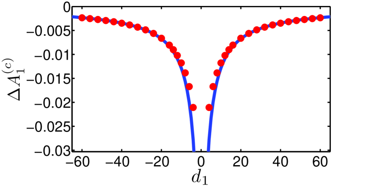
Figure 1: (Color online) The collision-induced amplitude shift of pulse 1 $\Delta A_{1}^{(c)}$ vs group velocity parameter $d_{1}$ in a fast collision between two Gaussian pulses in a linear waveguide with weak linear and cubic loss. The red circles correspond to the result obtained by simulations with Eq. (1). The solid blue line corresponds to the prediction of Eq. (17).

Figure 2 shows the dependence of $\Delta A_{1}^{(c)}$ on $d_{1}$ for fast collisions between two square pulses, as obtained by numerical simulations with Eq. (1). The analytic prediction of Eq. (18) is also shown. The agreement between the numerical simulations and the analytic prediction is very good. In particular, the relative error in the approximation is less than 11$\%$ for $|d_{1}|>10$ and less than 6$\%$ for $|d_{1}|>20$. At $|d_{1}|\simeq 4$, the relative error is 26$\%$. Similar results to the ones presented in Figs. 1 and 2 are obtained for other choices of the physical parameter values and for other pulse shapes. We therefore conclude that pulses of the linear propagation equation indeed exhibit soliton-like behavior in fast collisions in the presence of weak cubic loss.

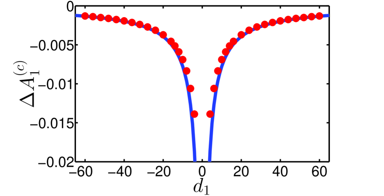
Figure 2: (Color online) The collision-induced amplitude shift of pulse 1 $\Delta A_{1}^{(c)}$ vs group velocity parameter $d_{1}$ in a fast collision between two square pulses in a linear waveguide with weak linear and cubic loss. The red circles correspond to the result obtained by simulations with Eq. (1). The solid blue line corresponds to the prediction of Eq. (18).

III Fast collisions in systems described by coupled linear diffusion-advection models

III.1 Evolution model

We now turn to describe the dynamics of fast collisions between pulses of two substances, denoted by 1 and 2, that evolve in the presence of linear diffusion and weak linear and quadratic loss. In addition, we assume that material 2 is advected with velocity $v_{d}$ relative to material 1. The dynamics of the two-pulse collision is described by the following system of perturbed coupled linear diffusion-advection equations:

$$\!\!\!\!\!\!\!\!\!\!\!\!\!\!\partial_{t}u_{1}=\partial_{x}^{2}u_{1}-\varepsilon_{1}u_{1}-\varepsilon_{2}u_{1}^{2}-2\varepsilon_{2}u_{1}u_{2},$$

$$\!\!\!\!\!\!\!\!\!\!\!\!\!\!\partial_{t}u_{2}=\partial_{x}^{2}u_{2}-v_{d}\partial_{x}u_{2}-\varepsilon_{1}u_{2}-\varepsilon_{2}u_{2}^{2}-2\varepsilon_{2}u_{1}u_{2},$$ (20)

where $u_{1}$ and $u_{2}$ are the concentrations of substance 1 and 2, $t$ is time, $x$ is a spatial coordinate, and $\varepsilon_{1}$ and $\varepsilon_{2}$ are the linear and quadratic loss coefficients, which satisfy $0<\varepsilon_{1}\ll 1$ and $0<\varepsilon_{2}\ll 1$ Dimensions2 . The term $-v_{d}\partial_{x}u_{2}$ in Eq. (20) describes advection, while the terms $-\varepsilon_{1}u_{j}$ correspond to linear loss. The terms $-\varepsilon_{2}u_{j}^{2}$ and $-2\varepsilon_{2}u_{j}u_{k}$ describe intra-substance and inter-substance effects due to quadratic loss, respectively.

III.2 Calculation of the amplitude shift in a fast two-pulse collision

We consider a fast collision between two pulses of substances 1 and 2 with generic shapes and with tails that exhibit exponential or faster than exponential decay. We assume that the pulses can be characterized by initial amplitudes $A_{j}(0)$, initial widths $W_{j0}$, and initial positions $x_{j0}$. Therefore, for a collision between two Gaussian pulses, for example, the initial concentrations are:

$$\!\!\!\!\!\!\!u_{j}(x,0)=A_{j}(0)\exp[-(x-x_{j0})^{2}/(2W_{j0}^{2})],\!\!\!\!\!\!\!\!$$ (21)

where $j=1,2$. Additionally, for a collision between two square pulses, the initial concentrations are:

$$\!\!\!\!\!\!\!\!\!u_{j}(x,0)=\left\{\begin{array}[]{l l}A_{j}(0)&\;\;\mbox{for}\;\;|x-x_{j0}|\leq W_{j0}/2,\\ 0&\;\;\mbox{for}\;\;|x-x_{j0}|>W_{j0}/2,\\ \end{array}\right.$$ (24)

where $j=1,2$. We assume a complete collision, that is, a collision in which the pulses are well separated at $t=0$ and at the final time $t=t_{f}$. The assumption of a fast collision means that the time interval $\Delta t_{c}=W_{0}/|v_{d}|$, along which the two pulses overlap, is much shorter than the diffusion time $t_{D}=W_{0}^{2}$. Requiring $\Delta t_{c}\ll t_{D}$, we obtain $W_{0}|v_{d}|\gg 1$, as the condition for a fast collision.

The perturbative calculation of the collision-induced amplitude shift is similar to the one carried out in section II.2 for fast collisions in linear waveguides with weak cubic loss. Thus, we look for a solution of Eq. (20) in the form

$$\!\!\!\!\!\!\!u_{j}(x,t)=u_{j0}(x,t)+\phi_{j}(x,t),$$ (25)

where $j=1,2$, $u_{j0}$ are solutions of Eq. (20) without inter-pulse interaction, and $\phi_{j}$ describe collision-induced effects. By definition, $u_{10}$ and $u_{20}$ satisfy the equations

$$\!\!\!\!\!\!\!\partial_{t}u_{10}=\partial_{x}^{2}u_{10}-\varepsilon_{1}u_{10}-\varepsilon_{2}u_{10}^{2},\!\!\!\!\!\!\!\!$$ (26)

and

$$\!\!\!\!\!\!\!\partial_{t}u_{20}=\partial_{x}^{2}u_{20}-v_{d}\partial_{x}u_{20}-\varepsilon_{1}u_{20}-\varepsilon_{2}u_{20}^{2}.\!\!\!\!\!\!\!\!$$ (27)

We substitute relation (25) into Eq. (20) and use Eqs. (26) and (27) to obtain equations for $\phi_{1}$ and $\phi_{2}$. We concentrate on the calculation of $\phi_{1}$, as the calculation of $\phi_{2}$ is similar. Taking into account only leading-order effects of the collision, we can neglect terms of the form $-\varepsilon_{1}\phi_{1}$, $-2\varepsilon_{2}u_{10}\phi_{1}$, $-2\varepsilon_{2}u_{20}\phi_{1}$, $-2\varepsilon_{2}u_{10}\phi_{2}$, etc. We therefore obtain:

$$\partial_{t}\phi_{1}=\partial_{x}^{2}\phi_{1}-2\varepsilon_{2}u_{10}u_{20}.$$ (28)

The term $-2\varepsilon_{2}u_{10}u_{20}$ on the right hand side of Eq. (28) is of order $\varepsilon_{2}$. Equating the orders of $\partial_{t}\phi_{1}$ and $-2\varepsilon_{2}u_{10}u_{20}$ and taking into account that $\Delta t_{c}$ is of order $1/|v_{d}|$, we find that $\phi_{1}$ is of order $\varepsilon_{2}/|v_{d}|$. In addition, the term $\partial_{x}^{2}\phi_{1}$, which is of order $\varepsilon_{2}/|v_{d}|$, can be neglected. Therefore, in the leading order, the equation for the collision-induced change of pulse 1 is:

$$\partial_{t}\phi_{1}=-2\varepsilon_{2}u_{10}u_{20}.$$ (29)

Equation (29) is similar to Eq. (11) and also to the equation obtained in Ref. PNC2010 for a fast collision between two optical solitons in a nonlinear optical waveguide with weak cubic loss.

We calculate the collision-induced amplitude shift of pulse 1 from the collision-induced change in the concentration of pulse 1. For this purpose, we denote by $t_{c}$ the collision time, i.e., the time at which the maxima of $u_{j}(x,t)$ coincide. In a fast collision, the collision takes place in a small time interval $[t_{c}-\Delta t_{c},t_{c}+\Delta t_{c}]$ about $t_{c}$. Therefore, the net collision-induced change in the concentration of pulse 1 $\Delta\phi_{1}(x,t_{c})$ can be evaluated by: $\Delta\phi_{1}(x,t_{c})=\phi_{1}(x,t_{c}+\Delta t_{c})-\phi_{1}(x,t_{c}-\Delta t_{c})$. To calculate $\Delta\phi_{1}(x,t_{c})$, we use the approximation: $u_{j0}(x,t)=A_{j}(t)\tilde{u}_{j0}(x,t)$, where $\tilde{u}_{j0}(x,t)$ is the solution of the diffusion equation without linear and quadratic loss and with $A_{j}(0)=1$. Substituting the approximate expressions for $u_{j0}$ into Eq. (29) and integrating with respect to time over the interval $[t_{c}-\Delta t_{c},t_{c}+\Delta t_{c}]$, we obtain:

$$\!\!\!\!\!\!\!\!\!\!\!\Delta\phi_{1}(x,t_{c})\!=\!-2\varepsilon_{2}\!\!\int_{t_{c}-\Delta t_{c}}^{t_{c}+\Delta t_{c}}\!\!\!\!\!\!\!\!\!\!\!\!\!\!\!\!dt^{\prime}A_{1}(t^{\prime})A_{2}(t^{\prime})\tilde{u}_{10}(x,t^{\prime})\tilde{u}_{20}(x,t^{\prime}).$$

(30)

The only function on the right hand side of Eq. (30) that contains fast variations in $t$, which are of order 1, is $\tilde{u}_{20}$. Therefore, we can approximate $A_{1}(t)$, $A_{2}(t)$, and $\tilde{u}_{10}(x,t)$ by $A_{1}(t_{c}^{-})$, $A_{2}(t_{c}^{-})$, and $\tilde{u}_{10}(x,t_{c})$. Additionally, we can take into account only the fast dependence of $\tilde{u}_{20}$ on $t$, i.e., the $t$ dependence that is contained in factors of the form $y=x-x_{20}-v_{d}t$. Denoting this approximation of $\tilde{u}_{20}(x,t)$ by $\bar{u}_{20}(y,t_{c})$, we obtain:

$$\!\!\!\!\!\!\!\!\!\!\!\Delta\phi_{1}(x,t_{c})\!=\!-2\varepsilon_{2}A_{1}(t_{c}^{-})A_{2}(t_{c}^{-})\tilde{u}_{10}(x,t_{c})\times$$

$$\!\!\!\int_{t_{c}-\Delta t_{c}}^{t_{c}+\Delta t_{c}}\!\!\!\!\!\!\!\!dt^{\prime}\bar{u}_{20}(x-x_{20}-v_{d}t^{\prime},t_{c}).$$ (31)

The integrand on the right hand side of Eq. (31) is sharply peaked at a small interval about $t_{c}$. Therefore, we can extend the limits of the integral to $-\infty$ and $\infty$. In addition, we change the integration variable from $t^{\prime}$ to $y=x-x_{20}-v_{d}t^{\prime}$ and obtain

$$\!\!\!\!\!\!\Delta\phi_{1}(x,t_{c})=-\frac{2\varepsilon_{2}A_{1}(t_{c}^{-})A_{2}(t_{c}^{-})}{|v_{d}|}\tilde{u}_{10}(x,t_{c})\!\!\!\int_{-\infty}^{\infty}\!\!\!\!\!\!\!\!dy\,\bar{u}_{20}(y,t_{c}).$$

(32)

The total collision-induced amplitude shift of pulse 1 $\Delta A_{1}^{(c)}$ is related to the collision-induced change in the concentration of the pulse $\Delta\phi_{1}(x,t_{c})$ by:

$$\!\!\!\!\!\!\!\!\!\!\!\!\!\!\Delta A_{1}^{(c)}=\left[\int_{-\infty}^{\infty}\!\!\!\!\!dx\,\tilde{u}_{10}(x,t_{c})\right]^{-1}\!\!\int_{-\infty}^{\infty}\!\!\!\!\!dx\,\Delta\phi_{1}(x,t_{c})$$ (33)

(see Appendix A). Substituting Eq. (32) into Eq. (33), we find that the total collision-induced amplitude shift of pulse 1 is:

$$\!\!\!\!\!\!\!\!\Delta A_{1}^{(c)}=-\frac{2\varepsilon_{2}A_{1}(t_{c}^{-})A_{2}(t_{c}^{-})}{|v_{d}|}\int_{-\infty}^{\infty}dy\,\bar{u}_{20}(y,t_{c}).$$ (34)

Equation (34) is expected to hold for generic pulse shapes $u_{j0}(x,t)$ with tails that exhibit exponential or faster than exponential decay. Using Eq. (34) for a fast collision between two Gaussian pulses with initial widths $W_{j0}$, we find that the collision-induced amplitude shift in this case is given by:

$$\!\!\!\!\!\!\!\!\Delta A_{1}^{(c)}=-(8\pi)^{1/2}\varepsilon_{2}W_{20}A_{1}(t_{c}^{-})A_{2}(t_{c}^{-})/|v_{d}|.$$ (35)

In a similar manner, we find that the collision-induced amplitude shift in a fast collision between two square pulses with initial widths $W_{j0}$ is:

$$\!\!\!\!\!\!\!\!\Delta A_{1}^{(c)}=-2\varepsilon_{2}W_{20}A_{1}(t_{c}^{-})A_{2}(t_{c}^{-})/|v_{d}|.$$ (36)

Equations (35) and (36) are similar to Eqs. (17) and (18) for the collision-induced amplitude shift in linear waveguides with weak cubic loss. Equations (35) and (36) are also similar to Eq. (19) for the amplitude shift in a fast two-soliton collision in a nonlinear optical waveguide with weak cubic loss. Based on the similar forms of Eqs. (34)-(36) and Eq. (19) we conclude that pulses in linear physical systems described by the diffusion-advection model (20) exhibit soliton-like behavior in fast collisions.

III.3 Numerical simulations

To check the predictions for soliton-like behavior in the collisions, we carry out numerical simulations with Eq. (20). The equation is numerically solved by the split-step method with periodic boundary conditions Verwer2003 . For concreteness, we present here the results of simulations with parameter values $\varepsilon_{1}=0.01$ and $\varepsilon_{2}=0.01$. The values of $v_{d}$ are varied in the intervals $-60\leq v_{d}\leq-4$ and $4\leq v_{d}\leq 60$. We carry out the simulations for two cases: (1) collisions between two Gaussian pulses; (2) collisions between two square pulses. The initial condition in the first case consists of two Gaussian pulses of the form (21) with parameter values $A_{j}(0)=1$, $W_{j0}=4$, $x_{10}=0$, and $x_{20}=\pm 20$. The initial condition in the second case consists of two square pulses of the form (24) with parameter values $A_{j}(0)=1$, $W_{j0}=4$, $x_{10}=0$, and $x_{20}=\pm 10$. The numerical and theoretical values of $\Delta A_{1}^{(c)}$ are calculated by the same methods that were used for the linear waveguide system.

Figure 3 shows the dependence of the collision-induced amplitude shift $\Delta A_{1}^{(c)}$ on $v_{d}$ for fast collisions between two Gaussian pulses, as obtained by simulations with Eq. (20). The analytic prediction of Eq. (35) is also shown. The agreement between the result of the simulations and the analytic prediction is very good. Indeed, the relative error is less than 9$\%$ for $|v_{d}|>10$ and less than 3$\%$ for $|v_{d}|>20$. Even at $|v_{d}|\simeq 4$, the relative error is only 20$\%$.

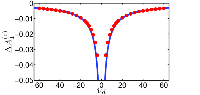
Figure 3: (Color online) The collision-induced amplitude shift of pulse 1 $\Delta A_{1}^{(c)}$ vs advection velocity $v_{d}$ in a fast collision between two Gaussian pulses in a system, described by the diffusion-advection model (20). The red circles correspond to the result obtained by simulations with Eq. (20). The solid blue line corresponds to the prediction of Eq. (35).

The dependence of the collision-induced amplitude shift $\Delta A_{1}^{(c)}$ on $v_{d}$ for fast collisions between two square pulses is shown in Figure 4. Both the result obtained by simulations with Eq. (20) and the analytic prediction of Eq. (36) are shown. The agreement between the result of the numerical simulations and the analytic prediction is very good. In particular, the relative error is less than 13$\%$ for $|v_{d}|>10$ and less than 6$\%$ for $|v_{d}|>20$. At $|v_{d}|\simeq 4$, the relative error is 33$\%$. Similar results to the ones presented in Figs. 3 and 4 are obtained for other physical parameter values and for other pulse shapes. Based on these results, we conclude that pulses in linear systems, described by diffusion-advection models, indeed exhibit soliton-like behavior in fast collisions in the presence of weak quadratic loss.

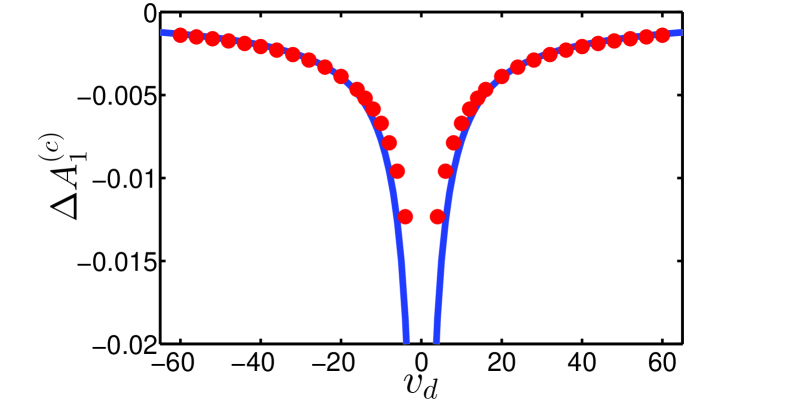
Figure 4: (Color online) The collision-induced amplitude shift of pulse 1 $\Delta A_{1}^{(c)}$ vs advection velocity $v_{d}$ in a fast collision between two square pulses in a system, described by the diffusion-advection model (20). The red circles correspond to the result obtained by simulations with Eq. (20). The solid blue line corresponds to the prediction of Eq. (36).

IV Conclusions

We demonstrated that pulses of linear physical systems, weakly perturbed by nonlinear dissipation, exhibit soliton-like behavior in fast collisions. The behavior was demonstrated for linear waveguides with weak cubic loss and for systems described by linear diffusion-advection models with weak quadratic loss. We showed that in both systems, the expressions for the collision-induced amplitude shifts due to the nonlinear loss have the same form as the expression for the amplitude shift in a fast collision between two optical solitons in a nonlinear optical waveguide with weak cubic loss. Our analytic predictions are confirmed by numerical simulations with the corresponding coupled linear evolution models with weak nonlinear loss. These results show that conclusions drawn from analysis of fast two-soliton collisions in the presence of weak dissipation can be applied for understanding the dynamics of fast two-pulse collisions in a large class of weakly perturbed linear physical systems, even though the pulses in the linear systems are not shape preserving. Furthermore, our results open the way for studying dynamics of fast collisions between pulses of weakly perturbed linear physical systems in an arbitrary spatial dimension, which is typically impossible for collisions between solitons in systems described by nonlinear Schrödinger models, due to the instability of the solitons in dimension higher than one.

Author contribution statement

All authors contributed to this work equally.

Appendix A Calculation of $\Delta A_{1}^{(c)}$ from $\Delta\Phi_{1}(t,z_{c})$ and $\Delta\phi_{1}(x,t_{c})$

In this Appendix, we derive relations (15) and (33) between the collision-induced amplitude shift $\Delta A_{1}^{(c)}$ and the collision-induced changes in the envelopes of the electric field and in material concentration $\Delta\Phi_{1}(t,z_{c})$ and $\Delta\phi_{1}(x,t_{c})$. These relations were used to obtain Eq. (16) and Eq. (34) for $\Delta A_{1}^{(c)}$ from Eqs. (14) and (32), respectively.

We start by considering the linear waveguide system with weak linear and cubic loss, described by Eq. (1). Employing the relation $\psi_{1}(t,z_{c})=\psi_{10}(t,z_{c})+\Delta\phi_{1}(t,z_{c})$, we obtain:

$$\!\!\!\!\!\!\!\!\!\!\!\!\!\!\!\!\int_{-\infty}^{\infty}\!\!\!\!\!\!\!\!dt|\psi_{1}(t,z_{c})|^{2}=\int_{-\infty}^{\infty}\!\!\!\!\!\!\!\!dt|\psi_{10}(t,z_{c})+\Delta\phi_{1}(t,z_{c})|^{2}.$$ (37)

Using the definitions of $\Psi_{10}$, $\tilde{\Psi}_{10}$, and $\Delta\Phi_{1}$, in Eq. (37), we obtain:

$$\!\!\!\!\!\!\!\!\!\!\!\!\int_{-\infty}^{\infty}\!\!\!\!\!\!\!\!dt|\psi_{1}(t,z_{c})|^{2}\!=\!\!\!\int_{-\infty}^{\infty}\!\!\!\!\!\!\!\!dt\left[A_{1}(z_{c}^{-})\tilde{\Psi}_{10}(t,z_{c})\!+\!\Delta\Phi_{1}(t,z_{c})\right]^{2}\!\!\!\!.$$ (38)

Expanding the integrand on the right hand side of Eq. (38), while keeping only the first two leading terms, we arrive at:

$$\!\!\!\!\!\!\!\!\!\int_{-\infty}^{\infty}\!\!\!\!\!\!\!\!dt|\psi_{1}(t,z_{c})|^{2}\simeq C_{1}A_{1}^{2}(z_{c}^{-})$$

$$+2A_{1}(z_{c}^{-})\int_{-\infty}^{\infty}\!\!\!\!\!\!\!\!dt\tilde{\Psi}_{10}(t,z_{c})\Delta\Phi_{1}(t,z_{c}),$$ (39)

where $C_{1}=\int_{-\infty}^{\infty}\!\!\!dt\tilde{\Psi}_{10}^{2}(t,z_{c})$ is a constant coll_conserved . On the other hand, we can write:

$$\!\!\!\!\!\!\!\!\!\int_{-\infty}^{\infty}\!\!\!\!\!\!\!\!dt|\psi_{1}(t,z_{c})|^{2}\!=\!\left(A_{1}(z_{c}^{-})+\Delta A_{1}^{(c)}\right)^{2}\int_{-\infty}^{\infty}\!\!\!\!\!\!\!\!dt\tilde{\Psi}_{10}^{2}(t,z_{c})$$

$$\simeq C_{1}A_{1}^{2}(z_{c}^{-})+2C_{1}A_{1}(z_{c}^{-})\Delta A_{1}^{(c)}.$$ (40)

Equating the right hand sides of Eqs. (39) and (40), we obtain:

$$\!\!\!\!\!\!\!\!\!\Delta A_{1}^{(c)}=\frac{1}{C_{1}}\int_{-\infty}^{\infty}\!\!\!\!\!\!\!\!dt\tilde{\Psi}_{10}(t,z_{c})\Delta\Phi_{1}(t,z_{c}),$$ (41)

which is the relation used to derive Eq. (16) from Eq. (14).

We now treat systems described by the coupled linear diffusion-advection model (20). Using the relation $u_{1}(x,t_{c})=u_{10}(x,t_{c})+\Delta\phi_{1}(x,t_{c})$, we obtain:

$$\!\!\!\!\!\!\!\!\!\!\!\!\!\!\!\!\int_{-\infty}^{\infty}\!\!\!\!\!\!\!\!dx\,u_{1}(x,t_{c})=\int_{-\infty}^{\infty}\!\!\!\!\!\!\!\!dx\left[u_{10}(x,t_{c})+\Delta\phi_{1}(x,t_{c})\right].$$ (42)

From the definition of $\tilde{u}_{10}(x,t_{c})$ it follows that

$$\!\!\!\!\!\!\!\!\!\!\!\!\!\!\!\!\int_{-\infty}^{\infty}\!\!\!\!\!\!\!\!dx\,u_{1}(x,t_{c})=C_{2}A_{1}(t_{c}^{-})+\int_{-\infty}^{\infty}\!\!\!\!\!\!\!\!dx\,\Delta\phi_{1}(x,t_{c}),$$ (43)

where $C_{2}=\int_{-\infty}^{\infty}\!\!\!\!\!dx\tilde{u}_{10}(x,t_{c})$ is a constant rda_conserved . On the other hand, we can write:

$$\!\!\!\!\!\!\!\!\!\!\!\!\!\!\!\!\int_{-\infty}^{\infty}\!\!\!\!\!\!\!\!dx\,u_{1}(x,t_{c})=\left(A_{1}(t_{c}^{-})+\Delta A_{1}^{(c)}\right)\int_{-\infty}^{\infty}\!\!\!\!\!\!\!\!dx\,\tilde{u}_{10}(x,t_{c})$$

$$=C_{2}A_{1}(t_{c}^{-})+C_{2}\Delta A_{1}^{(c)}.$$ (44)

Equating the right hand sides of Eqs. (43) and (44), we obtain:

$$\!\!\!\!\!\!\!\!\!\Delta A_{1}^{(c)}=\frac{1}{C_{2}}\int_{-\infty}^{\infty}\!\!\!\!\!\!\!\!dx\,\Delta\phi_{1}(x,t_{c}),$$ (45)

which is the relation used to derive Eq. (34) from Eq. (32).

Appendix B Procedures for calculating the values of $\Delta A_{1}^{(c)}$ from the analytic predictions and from numerical simulations

Let us describe the procedures used for calculating the values of the collision-induced amplitude shift $\Delta A_{1}^{(c)}$ from the analytic predictions and from results of numerical simulations. For concreteness, we demonstrate the implementation of these procedures for a collision between two Gaussian pulses in linear optical waveguides with weak linear and cubic loss. The implementation for collisions between pulses with other shapes and for collisions in physical systems described by linear diffusion-advection models is similar.

The analytic prediction for $\Delta A_{1}^{(c)}$ is obtained by employing Eq. (17). The values of $A_{j}(z_{c}^{-})$ are calculated by solving an approximate equation for the dynamics of $A_{j}(z)$ for a single pulse, propagating in the presence of first and second-order dispersion, linear loss, and cubic loss. More specifically, using an energy balance calculation for this single-pulse propagation problem, we obtain

$$\!\!\!\!\!\!\!\!\!\!\!\!\partial_{z}\int_{-\infty}^{\infty}\!\!\!\!\!\!dt|\psi_{j}|^{2}\!=\!-2\epsilon_{1}\int_{-\infty}^{\infty}\!\!\!\!\!\!dt|\psi_{j}|^{2}-2\epsilon_{3}\int_{-\infty}^{\infty}\!\!\!\!\!\!dt|\psi_{j}|^{4}.$$ (46)

We express the approximate solution of the propagation equation as $\psi_{j}(t,z)=A_{j}(z)\tilde{\Psi}_{j0}(t,z)\exp[i\chi_{j0}(t,z)]$, where $\tilde{\Psi}_{j0}(t,z)\exp[i\chi_{j0}(t,z)]$ is the solution of the propagation equation in the absence of linear and cubic loss with initial amplitude $A_{j}(0)=1$. Substituting the relation for $\psi_{j}(t,z)$ into Eq. (46), we obtain:

$$\!\!\!\!\!\!\!\!\!\!\!\!\frac{d}{dz}\left[I_{2}A_{j}^{2}\right]=-2\epsilon_{1}I_{2}A_{j}^{2}-2\epsilon_{3}I_{4}(z)A_{j}^{4}\,,$$ (47)

where $I_{2}=\int_{-\infty}^{\infty}\!\!\!dt\tilde{\Psi}_{j0}^{2}(t,z)=\int_{-\infty}^{\infty}\!\!\!dt\tilde{\Psi}_{j0}^{2}(t,0)$ and $I_{4}(z)=\int_{-\infty}^{\infty}\!\!\!dt\tilde{\Psi}_{j0}^{4}(t,z)$. For Gaussian pulses with initial width $W_{j0}$, we find $I_{2}=\pi^{1/2}W_{j0}$ and $I_{4}(z)=\pi^{1/2}W_{j0}^{3}/[2(W_{j0}^{4}+4z^{2})]^{1/2}$. Using these relations in Eq. (47), we arrive at

$$\!\!\!\!\!\!\!\!\!\!\!\!\frac{d}{dz}\left(A_{j}^{2}\right)+2\epsilon_{1}A_{j}^{2}=-\frac{2^{1/2}\epsilon_{3}W_{j0}^{2}A_{j}^{4}}{(W_{j0}^{4}+4z^{2})^{1/2}}\,.$$ (48)

The solution of Eq. (48) on the interval $[0,z]$ is

$$\!\!\!\!\!\!\!\!\!\!\!\!A_{j}(z)=\frac{A_{j}(0)e^{-\epsilon_{1}z}}{\left[1+2^{1/2}\epsilon_{3}W_{j0}^{2}\tilde{I}(0,z)A_{j}^{2}(0)\right]^{1/2}}\,,$$ (49)

where

$$\!\!\!\!\!\!\!\!\!\!\!\!\tilde{I}(y_{1},y_{2})=\int_{y_{1}}^{y_{2}}\frac{dy\,e^{-2\epsilon_{1}y}}{(W_{j0}^{4}+4y^{2})^{1/2}}\,.$$ (50)

We use Eq. (49) for calculating the values of $A_{j}(z_{c}^{-})$. Substitution of these values into Eq. (17) yields the analytic prediction for $\Delta A_{1}^{(c)}$.

To calculate $\Delta A_{1}^{(c)}$ from the simulations, we need to separate the collision-induced amplitude shift from the amplitude shift due to single-pulse propagation. The procedure that we adopt is a generalization of the method used in Refs. PNC2010 and PC2012 for calculating the collision-induced amplitude shift in two-soliton collisions in the presence of nonlinear loss. More specifically, we calculate the value of $\Delta A_{1}^{(c)}$ from the simulations by using $\Delta A_{1}^{(c)}=A_{1}(z_{c}^{+})-A_{1}(z_{c}^{-})$, where $A_{j}(z_{c}^{+})$ is the limit from the right of $A_{j}$ at $z_{c}$. The values of $A_{1}(z_{c}^{-})$ and $A_{1}(z_{c}^{+})$ are obtained by solving Eq. (48) on the intervals $[z_{1},z_{c}]$ and $[z_{c},z_{2}]$, where $z_{1}$ and $z_{2}$ are the distances at which the collision effectively starts and ends, respectively. We estimates these distances by $z_{1}=z_{c}-a/|d_{1}|$ and $z_{2}=z_{c}+a/|d_{1}|$, where $a>0$ is a constant of the same order of magnitude as $W_{j0}$. The expressions obtained in this manner are:

$$\!\!\!\!\!\!\!\!\!\!\!\!A_{1}(z_{c}^{-})=\frac{A_{1}(z_{1})e^{-\epsilon_{1}z_{c}}}{\left[e^{-2\epsilon_{1}z_{1}}+2^{1/2}\epsilon_{3}W_{j0}^{2}\tilde{I}(z_{1},z_{c})A_{1}^{2}(z_{1})\right]^{1/2}},$$ (51)

and

$$\!\!\!\!\!\!\!\!\!\!\!\!A_{1}(z_{c}^{+})=\frac{A_{1}(z_{2})e^{-\epsilon_{1}z_{c}}}{\left[e^{-2\epsilon_{1}z_{2}}-2^{1/2}\epsilon_{3}W_{j0}^{2}\tilde{I}(z_{c},z_{2})A_{1}^{2}(z_{2})\right]^{1/2}}.$$ (52)

Thus, we obtain the values of $A_{1}(z_{c}^{-})$ and $A_{1}(z_{c}^{+})$ by using Eqs. (51) and (52) with values of $A_{1}(z_{1})$ and $A_{1}(z_{2})$, which are measured from the simulations.

References

- (1) S. Novikov, S.V. Manakov, L.P. Pitaevskii, and V.E. Zakharov, Theory of Solitons: The Inverse Scattering Method (Plenum, New York, 1984).
- (2) Y.S. Kivshar and B.A. Malomed, Rev. Mod. Phys. 61, 763 (1989).
- (3) G.P. Agrawal, Nonlinear Fiber Optics (Academic, San Diego, CA, 2001).
- (4) L.F. Mollenauer and J.P. Gordon, Solitons in Optical Fibers: Fundamentals and Applications (Academic, San Diego, CA, 2006).
- (5) W. Horton and Y.H. Ichikawa, Chaos and Structure in Nonlinear Plasmas (World Scientific, Singapore, 1996).
- (6) L.F. Mollenauer and P.V. Mamyshev, IEEE J. Quantum Electron. 34, 2089 (1998).
- (7) Y. Chung and A. Peleg, Nonlinearity 18, 1555 (2005).
- (8) A. Peleg, Q.M. Nguyen, and Y. Chung, Phys. Rev. A 82, 053830 (2010).
- (9) S. Chi and S. Wen, Opt. Lett. 14, 1216 (1989).
- (10) B.A. Malomed, Phys. Rev. A 44, 1412 (1991).
- (11) S. Kumar, Opt. Lett. 23, 1450 (1998).
- (12) A. Peleg, Opt. Lett. 29, 1980 (2004).
- (13) Q.M. Nguyen and A. Peleg, J. Opt. Soc. Am. B 27, 1985 (2010).
- (14) A. Peleg and Y. Chung, Phys. Rev. A 85, 063828 (2012).
- (15) F. Forghieri, R.W. Tkach, and A.R. Chraplyvy, in Optical Fiber Telecommunications III, I.P. Kaminow and T.L. Koch, eds., (Academic, San Diego, CA, 1997), Chapter 8.
- (16) G.P. Agrawal, P.L. Baldeck, and R.R. Alfano, Phys. Rev. A 39, 3406 (1989).
- (17) G.P. Agrawal, P.L. Baldeck, and R.R. Alfano, Opt. Lett. 14, 137 (1989).
- (18) A. Peleg, M. Chertkov, and I. Gabitov, Phys. Rev. E 68, 026605 (2003).
- (19) A. Peleg, M. Chertkov, and I. Gabitov, J. Opt. Soc. Am. B 21, 18 (2004).
- (20) J. Soneson and A. Peleg, Physica D 195, 123 (2004).
- (21) Q. Lin, O.J. Painter, and G.P. Agrawal, Opt. Express 15, 16604 (2007).
- (22) The dimensionless distance in Eq. (1) is , where is the dimensional distance, is the dispersion length, and is the pulse width. The dimensionless time is , where is time. , where is the electric field of the th pulse and is peak power. , where and is the group velocity of the th pulse. and , where and are the dimensional linear and cubic loss coefficients.
- (23) The dimensionless coordinate in Eq. (20) is , where is the dimensional coordinate, and is a reference pulse width. The dimensionless time is , where is time, , and is the diffusion coefficient. , where is the concentration of substance and is the peak concentration. , where is the dimensional advection velocity. and , where and are the dimensional linear and quadratic loss coefficients.
- (24) W.H. Hundsdorfer and J.G. Verwer, Numerical Solution of Time Dependent Advection-Diffusion-Reaction Equations (Springer, New York, 2003).
- (25) Since the integral is conserved by the unperturbed linear propagation equation, we can write: .
- (26) Since the integral is conserved by the unperturbed linear diffusion equation, we can write: