“SHORT”er Reasoning About
Larger Requirements Models

Abstract

When Requirements Engineering(RE) models are unreasonably complex, they cannot support efficient decision making. SHORT is a tool to simplify that reasoning by exploiting the “key” decisions within RE models. These “keys” have the property that once values are assigned to them, it is very fast to reason over the remaining decisions. Using these “keys”, reasoning about RE models can be greatly SHORTened by focusing stakeholder discussion on just these key decisions.

This paper evaluates the SHORT tool on eight complex RE models. We find that the number of keys are typically only 12% of all decisions. Since they are so few in number, keys can be used to reason faster about models. For example, using keys, we can optimize over those models (to achieve the most goals at least cost) two to three orders of magnitude faster than standard methods. Better yet, finding those keys is not difficult: SHORT runs in low order polynomial time and terminates in a few minutes for the largest models.

I Introduction

Many researchers [1, 2, 3, 4, 5, 6, 7, 8] report that the process of building and analyzing requirements models help stakeholders better understand the ramifications of their decisions. However, complex models can overwhelm stakeholders. Consider a committee reviewing the goal model shown in Fig. 1, that describes the information needs of a university computer science department [9]. This committee may have trouble with manually reasoning about all the conflicting relationships in this model. Further, automatic methods for the same task are hard to scale: as discussed below, reasoning about inference over these models is an NP-hard task.

But are models like Fig. 1 as complex as they appear? That graph is somewhat of a tangle—if we straightened out all the dependencies, would we find that the model depends on just a few key decisions? As shown below, such keys have been seen in other domains [10, 11, 12, 13]. This paper argues that it is beneficial to look for these keys. If they exist, we can achieve “shorter” reasoning about large RE models, where “shorter” means (a) large models can be processed in a very short time; (b) stakeholders can get faster feedback from their models; (c) stakeholders can conduct shorter debates about their models since they only need to debate a few key decisions.

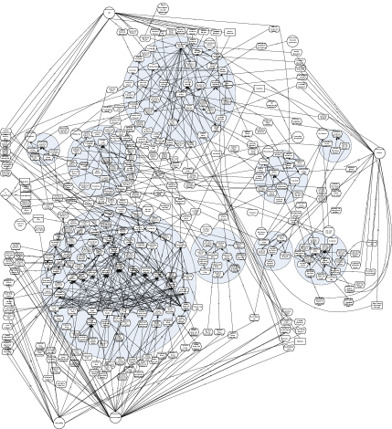
Figure 1: Options for services in a CS department (i* format). If the reader finds this model confusing, then our point is made.

The rest of this paper hunts for keys in RE models. Our next section offers a formal definition of keys, plus a simple introductory example where dozens of decisions are controlled by just three keys. Next, a review of the AI literature will show that that many models are known to have keys. After that, we introduce SHORT, a novel toolkit for finding and using keys. SHORT is then tested on eight RE models from the i* community [6] (see goo.gl/K7N6PE).

Figure 2: A requirements model for IT System modernization. This model has the syntax of Fig. 3. The three keys of this model are the leaf nodes shown in red and green (see text for an explanation of why these are the keys).

From those experiments, we conclude that keys can be found in numerous RE models since, in the sample of models explored here, the number of keys per model is small: typically 12% of all decisions. Also, keys are easy to find. SHORT runs in low-order polynomial time and terminates in just a few minutes (even for our largest model). This is a significant result: all prior attempts suffered from crippling runtimes that prevented scale up [14, 15]. Further, it is very useful to apply keys for reasoning about RE models. Using the keys, SHORT can find decisions that satisfy the most goals at the least cost, 100s to 1000s times faster than standard methods. Further, the decisions found by SHORT are competitive with (and sometimes even better than) those found by standard optimizers.

II “Keys”: Definition and Example

Consider a model (e.g. Fig. 1 or Fig. 2) where objectives $O\in\{x,y,.....\}$ are determined by stakeholders’ decisions $D$. After randomly selecting decisions, we would see variance on the objectives $V_{O}$. We say that a small set of decisions $K\subseteq D$ ($|K|\ll|D|$) are key, if after fixing decisions $K$ and randomly assigning the rest of the decisions in $D-K$, the variance $V^{\prime}_{o}$ drops significantly, i.e., $V^{\prime}_{O}\ll V_{O}$.

Just to say the obvious: it is useful to explore the keys first since, once the keys are set, there is more certainty about the impact of the remaining decisions. Also, for models with discrete, not continuous output, entropy could be swapped for variance in the above definition.

For example, Fig. 2 shows a requirements model about IT System modernization tasks such as the Y2K problem (moving from 2 digit to 4 digit years); reacting to vendor decisions to end-of-life operating systems and database products; and improving architectural support for new capabilities (e.g., support for mobile devices). The model in Fig. 2 comments on the refactoring, re-architecting, and redesign of existing systems. The model has the syntax of Fig. 3. Note that the model has dozens of decisions and a few top-level goals shown circled top right: “Good Example …”, “Easily Share Data Internally”, “Modernize”. All of these nodes have a cost determined by stakeholders. If the stakeholders are not sure of the exact costs, we allow them to define a range, and then conduct Monte Carlo simulations that sample randomly across that range. That said, for the rest of this paper we assume that cost of all the decisions is sampled from a triangular distribution (in our modeling language, this is a simple facet to change).

The two red and one green decisions in Fig. 2 are keys. To see this, note that the right-hand-side of the model has no connection to the top goals. Hence, two sensible decisions for this model would be to deny the leaves marked in dark red, thus disabling the right tree. As to the left-hand-side of the model, the leaf marked in dark green (“J2EE specification”) selects the shortest left-hand-side sub-branch with the fewest leaves. If the goal is to achieve the most high-level goals (at least cost), then it is also sensible to take this single dark green leaf. Why? Well, making any other decision on the left-hand-side of the model will significantly add to the overall cost of the solution, since all those other decisions require multiple conjunctions of decisions. It should be noted that such a visual inspection can never be performed on larger models(like Fig. 1) with hundreds of nodes and numerous cross tree constraints.

It is reasonable to ask what to do if users reject this analysis and explore the deeper branches on the left hand side. In such a case, we would tell a requirements engineer that “minimizing cost" is not a primary goal of these users. SHORT could then be rerun, removing the “minimizing cost" goal. That would lead to new alternatives, to be debated by the stakeholders. Note that it would not be burdensome since, as shown later(in Section V), SHORT runs in just a few seconds.

1. Nodes: have labels and decisions are label assignments. 2. Edges: Con nodes connect to other nodes via one four edges types “makes, helps, hurts, breaks” with weights $E_{j}\in\{1,$½$,-$½$,-1\}$, respectively. 3. Node types: Nodes in a goal model can be of type leaf, combine, or contribute (com nodes have sub-types and, or). Leaf nodes are different to the rest since they have no children. On the other hand, when dealing with and,or nodes, it is expected to meet all,one (respectively) of the requirements in the child nodes. Con nodes divide into softgoals, which users are willing to surrender if need be, and hardgoals which users are more eager to achieve.

4. Labels: Nodes $N_{i}$ have labels $\{1,$½$,0,-$½$,-1\}$ for satisfied, partially satisfied, undefined, denied and partially denied. 5. Initially, labels are undefined and are then relabelled satisfied or denied by some labeling procedure (e.g. see Fig. 5) during which labels may temporarily labeled partially satisfied/denied.

Figure 3: Syntax of goal models.

III Related Work

III-A Complexity of Processing RE Models

Given multiple stakeholders writing assertions into a requirements model, it is likely that those stakeholders will generate models that can contain contradictions; i.e. incompatible assignments of labels to variables. For example, in Fig. 2, it would be a contradiction to assign satisfied and denied to the same variable.

In traditional logic, if some set of assertions generates a contradiction then all the assertions are discarded as inconsistent. But in requirements models, when inconsistencies are detected, it is standard practice to focus on zones of agreement and avoid the parts of the model leading to the inconsistencies. Nuseibeh lists several strategies for this approach [16] including ignoring (skip over edges that lead to contradictions); circumventing (“slip around” inconsistencies; i.e. if inference is blocked due to inconsistency, the inference can explore other avenues); and ameliorating (when conflicts cannot be avoided, it is prudent to try reduce the total number of conflicts). The problem with these tactics is that they can be very slow. Formally, the study of models with contradictions is the called “abductive reasoning”. Poole’s THEORIST system [17] offers a clean logical framework of such reasoning. In that framework, a goal graph is a theory that contains a small number of upper-most goals. When we reason about that theory, we make assumptions about either (a) initial facts or (b) how to resolve contradictory decisions. In the general case, only some subset of the theory can be used to achieve some of the goals using some of the assumptions without leading to contradictions (denoted $\bot$). That is:

$$\begin{array}[]{r@{~}c@{~}l}T~{}&\subseteq\hfil~{}&\mathit{theory}\\ A~{}&\subseteq\hfil~{}&\mathit{assumptions}\\ G~{}&\subseteq\hfil~{}&\mathit{goals}\\ T\wedge A~{}&\vdash\hfil~{}&G\\ T\wedge A~{}&\not\vdash\hfil~{}&\bot\end{array}$$ (1)

A world of belief is a solution that satisfies these invariants. For many years we have tried to find such worlds using a variety of methods. For example Menzies’ HT4 system [14] combined forward and backward chaining to generate worlds while Ernst et al. [15] used DeKleer’s ATMS (assumption-based truth-maintenance system) [18]. Those implementations suffered from cripplingly slow runtimes that scaled very poorly to larger models. Such slow runtimes are not merely a quirk of those implementations—rather they are fundamental to the process of exploring models with many contradictions. It is easy to see why: exploring all the the subsets in Equation 1 is a very slow process. Bylander et al. [19] and Abdelbar et al. [20] both confirm that abduction is NP-hard; i.e. when exploring all options within a requirements goal model, we should expect very slow runtimes.

III-B Reports of “Keys” in AI Research

Just because an inference task is NP-hard, that does not necessarily imply that task will always exhibit exponential runtimes. Numerous AI researchers studying NP-hard tasks report the existence of a small number of key variables that determine the behavior of the rest of the model. When such keys are present, then the problem of controlling an entire model simplifies to just the problem of controlling the keys.

Keys have been discovered in AI many times and called many different names: Variable subset selection, narrows, master variables, and backdoors. In the 1960s, Amarel observed that search problems contain narrows; i.e. tiny sets of variable settings that must be used in any solution [11]. Amarel’s work defined macros that encode paths between the narrows in the search space, effectively permitting a search engine to leap quickly from one narrow to another.

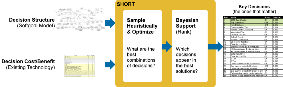
Figure 4: Finding solutions with SHORT. Costs and benefits are inputs are domain-specific constructs that, in our work, we develop with users as part the model elicitation process.

In later work, data mining researchers in the 1990s explored and examined what happens when a data miner deliberately ignores some of the variables in the training data. Kohavi and John report trials of data sets where up to 80% of the variables can be ignored without degrading classification accuracy [13]. Note the similarity with Amarel’s work: it is more important to reason about a small set of important variables than about all the variables.

At the same time, researchers in constraint satisfaction found “random search with retries” was a very effective strategy. Crawford and Baker reported that such searches took less time than a complete search to find more solutions using just a small number of retries [12]. Their ISAMP “iterative sampler” makes random choices within a model until it gets “stuck”; i.e. until further choices do not satisfy expectations. When “stuck”, ISAMP does not waste time fiddling with current choices (as was done by older chronological backtracking algorithms). Instead, ISAMP logs what decisions were made before getting “stuck”. It then performs a “retry”; i.e. resets and starts again, this time making other random choices to explore.

Crawford and Baker explain the success of this strange approach by assuming models contain a small set of master variables that set the remaining variables (and this paper calls such master variables keys). Rigorously searching through all variable settings is not recommended when master variables are present, since only a small number of those settings actually matter. Further, when the master variables are spread thinly over the entire model, it makes no sense to carefully explore all parts of the model since much time will be wasted “walking” between the far-flung master variables. For such models, if the reasoning gets stuck in one region, then the best thing to do is to leap at random to some distant part of the model.

A similar conclusion comes from the work of Williams et al. [10]. They found that if a randomized search is repeated many times, that a small number of variable settings were shared by all solutions. They also found that if they set those variables before conducting the rest of the search, then formerly exponential runtimes collapsed to low-order polynomial time. They called these shared variables the backdoor to reducing computational complexity.

Combining the above, we propose the following strategy for faster reasoning about RE models. First, use random search with retries to find the “key” decisions in RE models. Second, have stakeholders debate, and then decide, about the keys before exploring anything else. Third, to avoid trivially small solutions, our random search should strive to cover much of the model.

The rest of this paper implements this strategy in a tool called SHORT. This tool is a multi-objective optimizer that seeks to maximize goal satisfaction, while at the same time maximizing the softgoal satisfaction and minimizing the sum of the costs of the decisions made within that model.

IV Goal Inference with SHORT

As summarized in Fig. 4, SHORT runs in five phases:

• Sample Heuristically the possible labellings.

• Optimize the label assignments in order to cover more goals or reduce the sum of the cost of the decisions in the model. To implement the retry step recommended by Crawford and Baker’s ISAMP [12].

• Rank all decisions according to how well they performed during the optimization process.

• Test how much conclusions are determined by the decisions that occur very early in that ranking.

SH = Sample Heuristically: The SAMPLE procedure of Fig. 6 finds one possible set of consistent labels within a goal. The procedure calls the STEP procedure (Fig. 5) over all the decisions in the model, labeling as many nodes as possible. This procedure executes in a random order since (a) this emulates the idiosyncrasies of human discussions; (b) as mentioned above, Crawford and Baker found this to be a useful strategy for reducing computational complexity.

Why use SAMPLE when there are many other soft goal inference methods in the literature, such as e.g., the forwards and backwards analysis proposed by Horkoff and Yu [9]? One reason we prefer SAMPLE is its generality. SAMPLE was first developed for Menzies’ HT4 system and has been applied to many model types including a) causal diagrams; (b) qualitative equations; a (c) frame-based knowledge representation; (d) compartmental models, and even (e) first-order systems (with finite-domains on the variables) [21].

1. When considering an edge $E_{j}$ from $N_{i}$ to a child $N_{k}$ then: • If $N_{i}\in\{1,-1\}$ then expect $N_{k}=E_{j}*N_{i}$ else • If $E_{j}>0$ then expect $N_{k}=N_{i}$ else • If $E_{j}<0$ then expect $N_{k}=-N_{i}$. Goal model inference does not use a fuzzy set or probabilistic approach to reasoning about conflicting influences. Rather, goal edges are either used or ignored. Hence: 2. If $N_{k}$ is undefined, then it is labelled with the above expectations and we call STEP recursively over all edges to $N_{k}$’s children. Children are explored in a random order. After recursion, for and-nodes, labels get set back to undefined if any fail $N_{k}$ expectations (as defined by point #1). 3. Otherwise, if its label does not meet the above expectations, then we ignore the edge $E_{j}$.

Figure 5: Procedure STEP: labels neighboring nodes; may ignore some edges. Called by the SAMPLE procedure of Fig. 6.

1. SAMPLE inputs (a) a goal model and (b) a set of prior decisions made by any previous run of SAMPLE (so initially, this set is empty). 2. As it initializes, SAMPLE sets all nodes to undefined then all prior nodes to satisfied; 3. While there are undefined nodes, SAMPLE (1) “picks” one undefined decision as satisfied then (2) “reflects” over its edges using the STEP procedure of Fig. 5. SAMPLE is stochastic since “picks” and “reflects” return nodes and edges in a random order. 4. SAMPLE outputs a solution listing all satisfied nodes.

Important note: if prior is changed, then SAMPLE will return different solutions. That is, the results from SAMPLE can be carefully tuned and improved by the OPTIMIZE procedure of Fig. 7 that carefully selects useful priors.

Figure 6: Procedure SAMPLE: tries to labels many nodes. Called by the OPTIMIZE procedure of Fig. 7.

1. Given a model with $n$ decisions, OPTIMIZE calls SAMPLE $N=10*n$ times. Each call generates one member of the population popi∈N. 2. OPTIMIZE scores each popi according to various objective scores $o$. In the case of our goal models, the objectives are $o_{1}$ the sum of the cost of its decisions, $o_{2}$ the number of ignore edges, and the number of $o_{3}$ satisfied goals and $o_{4}$ softgoals. 3. OPTIMIZE tries to each replace popi with a mutant $q$ built by extrapolating between three other members of population $a,b,c$. At probability $p_{1}$, for each decision $a_{k}\in a$, then $m_{k}=a_{k}\vee(p_{1}<\mathit{rand}()\wedge(b_{k}\vee c_{k}))$. 4. Each mutant $m$ is assessed by calling $\text{SAMPLE}(\textit{model,prior=m})$; i.e. by seeing what can be achieved within a goal after first assuming that $\textit{prior}=m$. 5. To test if the mutant $m$ is preferred to popi, OPTIMIZE uses Zitler’s continuous domination cdom predicate [22]. This predicate compares two sets of objectives from sets $x$ and $y$. In that comparison, $x$ is better than another $y$ if $x$ “losses” least. In the following, $``n^{\prime\prime}$ is the number of objectives and $w_{j}\in\{-1,1\}$ shows if we seek to maximize $o_{j}$. $$\begin{array}[]{rcl}x\succ y&=&\textit{loss}(y,x)>\textit{loss}(x,y)\\ \textit{loss}(x,y)&=&\sum_{j}^{n}-e^{\Delta(j,x,y,n)}/n\\ \Delta(j,x,y,n)&=&w_{j}(o_{j,x}-o_{j,y})/n\end{array}$$ 5. OPTIMIZE repeatedly loops over the population, trying to replace items with mutants, until new better mutants stop being found.

Figure 7: Procedure OPTIMIZE: strives to find “good” priors which, when passes to SAMPLE, maximize the number of edges used while also minimizing cost, and maximizing satisfied hard goals and soft goals. OPTIMIZE is based on Storn’s differential evolution optimizer [23]. OPTIMIZE is called by the RANK procedure of Fig. 8. For the reader unfamiliar with the mutation technique of step 3 and the cdom scoring of step 5, we note that these are standard practice in the search-based SE community [24, 25].

O = Optimize: Fig. 6 discusses how we SAMPLE one set of labels from a softgoal model. As described at the bottom of that figure, that SAMPLE-ing process can be controlled via the prior decisions passed to the model. The OPTIMIZE procedure of Fig. 7 is a multi-objective evolutionary algorithm that learns which priors decisions lead to better labellings. Here, a better labelling produces (a) greater coverage of goals and softgoals, (b) minimization of skipped edges; (c) least cost solutions. Note: for this paper, we sample our decision costs from a triangular distribution (in future work, we will explore other distributions).

R= Rank: The RANK procedure of Fig. 8 reflects of the results of the optimizer to rank each decisions. Decisions are ranked by the probability that they are associated with the better goals. Note that the key decisions will be among the highest ranked decisions.

T = Test: The TEST procedure of Fig. 9 takes a ranked list of decisions, then tests what happens when the first few are fixed and the rest are selected at random.

1. Run OPTIMIZE $N=20$ times, keep all decisions $d$ in the generated population popi∈N and their objectives $o$. 2. For each objective $o_{j}\in o$, sort and separate the top 10% $o_{j}$ scores; call that “best” $b$ and the remainder “rest”. For each decision $d_{k}\in d$, do • Count how many times $n_{1}$ that $d_{k}$ is associated with a “best” objective score. Set $n_{2}=N-n_{1}$ • The value of $d_{k}$ for objective $o_{j}$ is the probability $p$ times the support $s$ that $d_{k}$ appears more often in “best” than “rest”. That is, $s_{j,k}=n_{1}*0.1$ and $p_{j,k}=(n_{1}*0.1)/(n_{1}*0.1+n_{2}*0.9)$. 3. Let ordering be all decisions, sorted descending by the value of decision $d_{k}$ across all objectives; i.e. $v_{k}=\sum_{j}s_{j,k}\times p_{j,k}$

Figure 8: Procedure RANK: ranks all decisions according to how well they performed during the optimization process. Used by the TEST procedure of Fig. 9.

1. Run RANK to get a sorted list of decisions $d$. 2. For all decisions $1\leq x\leq|d|$, do • Build a prior set using decisions $d_{1}..d_{x}$ from ordering; • 20 times, call SAMPLE(model, prior) • Record for position $x$ the median and IQR of the objectives found in those results. Aside: median= 50th percentile; IQR=(75th-25th) percentile.

Figure 9: Procedure TEST: from a ranked list of decisions $d$, set the first few decisions, then selected the rest at random.

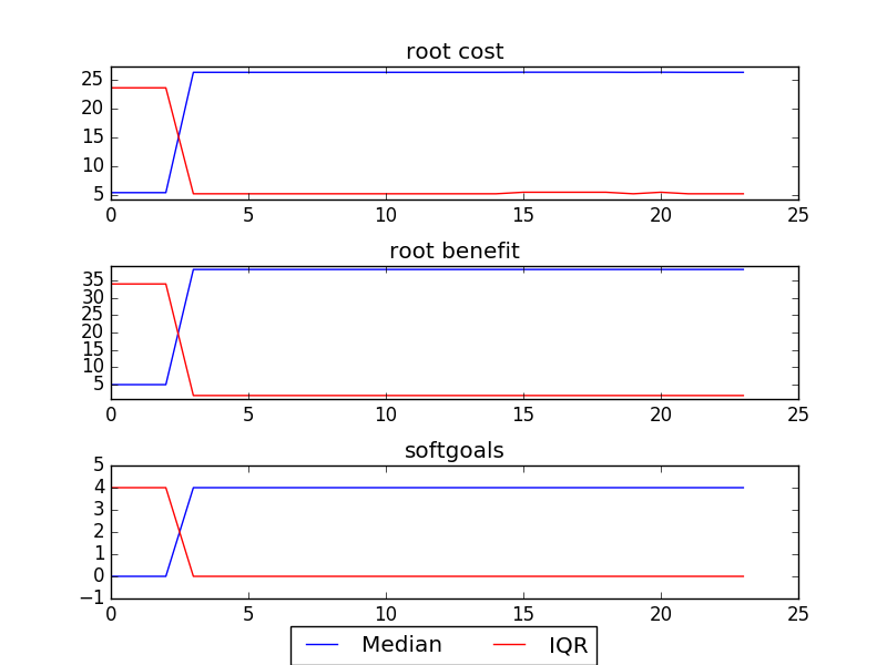
Figure 10: The X-axis contains $d$ decisions sorted by the RANK procedure of Fig. 8. The y-axis shows the results from the TEST procedure of Fig. 9; i.e. for $1\leq x\leq|d|$, fix the first $x$ decisions then, 20 times, make random choices about decisions $x+1$ to $|d|$. Results shown as median and IQR values. Median = 50% percentile and IQR=intra-quartile range= (75-25)th percentile. These results are smoothed such that these plots only change where this is statistically significant non-small change in the y-axis. An appendix to this paper describes our statistical smoothing procedure.

IV-A Reporting the Results

The SHORT process described above is a large-scale “what-if”+optimization procedure. In order to succinctly describe the results of the above, we apply the following statistical summarization method.

Fig. 10 shows what is reported by TEST after analyzing the modernization model of Fig. 2. At each point along the x-axis, TEST samples the goal model 20 times using prior decisions taken from $1\leq i\leq x$. In the solutions returned by SAMPLE, root cost is the sum of decision costs; root benefit/softgoals are the sum of the number of satisfied goals/soft goals. The blue and red plots show the median and variation around the median.

In these results, after making three decisions, the medians rise to a steady plateau and the variations plummet. That is, the model in Fig. 10 contains keys, as defined earlier in Section II.

This figure is reporting that this model has three key decisions which, if set, make further discussion superfluous. Note that these results match what we learned from a visual inspection of Fig. 2 in Section II.

1. J2EE Specification (satisfied) 2. Pnp Framework (denied) 3. New Database (denied) 4. Documentation Tool (satisfied) 5. Access Control Assessed (satisfied) 6. Monitoring Pilot (satisfied) 7. General Test Env (satisfied) 8. Bakeoff Result (satisfied) 9. Access Control Pilot (satisfied) 10. DB Vendor Test Env (satisfied) 11. Data Service Spec (satisfied) 12. External clients get their request (satisfied) 13. Co-ordinates & internal client (satisfied) 14. Co-ordinates & external client (satisfied) 15. Data Model Pilot (satisfied) 16. Data Service Pilot (satisfied) 17. 2 Tier (satisfied) 18. 3 Tier (satisfied) 19. Define data model for shared data (satisfied) 20. Svc layer w/ extracted biz logic (denied) 21. Define ext mandatory data std (satisfied) 22. Svc layer w/ extracted biz logic in DB (satisfied) 23. External data model can be extended (satisfied) 24. Provide logical data scheme internally (satisfied)

Figure 11: Results of decision ordering on Fig. 2. Read “satisfied/denied” as equivalent to ensuring that a leaf node is achieved or not achieved. Note the denied items at positions $x\in\{2,3,20\}$. These are recommendations of what not to do. The rest are all positive recommendations. The implication of Fig. 10 is that after following the recommendations for the first 3 decisions, the remaining decisions will have little additional impact on overall cost or satisfaction.

The decision rankings found by RANK for Fig. 2 are shown in Fig. 11. Two features of this list deserve comment. Firstly, this list is not 24 decisions that could inspire $2^{24}>16,000,000$ debates. Rather, it is an ordering with the property that item $x+1$ is recommended only if recommendations $1..x$ are first adopted. That is, this list offers only 24 decisions to users (if they choose to or not to perform actions $1..x$). Secondly, if users cannot implement all these recommendations, they can easily read from Fig. 10 the effects of implementing just the first $x$ items.

TABLE I: Goal models used in this study, sorted by number of edges.

Model	Nodes	Edges
Services	351	510	(see Fig. 1)
Counselling	350	470
Marketing	326	422
Management	206	239
ITDepartment	126	162
Kids&Youth	81	81
IT Modernization	53	57	(see Fig. 2)

V Validation: Looking for Keys in RE Models

We applied SHORT to 8 real-world RE models as an exploratory validation of our belief in the presence of keys in other RE models. We then compared SHORT to NSGA-II [26], a state-of-the-art optimizer.

The introductory model in Fig. 2 has 53 nodes and 57 edges. Table I shows some details on the other goal models used in this study. The largest of our sample is the CSServices models shown in Fig. 1. For images of all these models, see goo.gl/K7N6PE. These models were used since they are the largest publicly accessible RE models . All these models conform to the syntax defined in Fig. 3.

Model	Result	Percentage of Decisions
		0	6	12	25	50	100
Counselling	SGs	60	60	70	80	70	60
	Goals	50	60	70	60	70	40
	Costs	n.a.	5	10	20	28	35
Management	SGs	50	50	60	60	50	40
	Goals	50	50	50	60	60	60
	Costs	n.a.	4	8	20	24	32
Marketing	SGs	70	70	70	60	60	30
	Goals	70	70	70	70	60	40
	Costs	n.a.	6	8	11	12	20
ITDepartment	SGs	70	70	60	70	70	60
	Goals	60	50	50	80	80	70
	Costs	n.a.	2	4	9	17	18
SAProgram	SGs	80	80	80	80	80	80
	Goals	70	70	70	60	55	60
	Costs	n.a.	1	2	3	3	5
Services	SGs	50	50	50	50	50	50
	Goals	30	50	60	60	70	70
	Costs	n.a.	4	7	13	19	24
Kids&Youth	SGs	50	40	50	50	40	20
	Goals	50	50	70	60	60	70
	Costs	n.a.	0	0	4	7	10

TABLE II: Percentages of Softgoals and Goals covered, and total Costs, with respect to their maximum values after applying top 6,12,25,50,100% of decisions found and ranked by SHORT for the goal models of Table I.

Table II shows SHORT’s results after making the first 6,12,25,50,100% of the decisions along the ranking found by RANK. In a result consistent with Fig. 10, there is little change to goal or soft goal coverage are making just a few decisions: typically, just 12% of the decisions(see https://goo.gl/cRv9Lm).

Two exceptions to the pattern “12% is enough” are CSCounselling and ITDepartment. Those models achieved nearly max goal coverage at 12% but did not peak until making 25% of the decisions. Even with that exception, the general conclusion is clear: with SHORT, only a minority of the decisions need to be made with care, since once those are made, the goal coverage is robust (unchanging) for the remaining decisions.

(Aside: one quirk of Table II is that, as shown in the column headed with “0”, even when no decisions are made, it is possible to achieve some of the goals and softgoals, just by making decisions at random. Since no human has committed to any decision in that region, we mark all the 0% costs as “n.a.” to indicate that they are not applicable.)

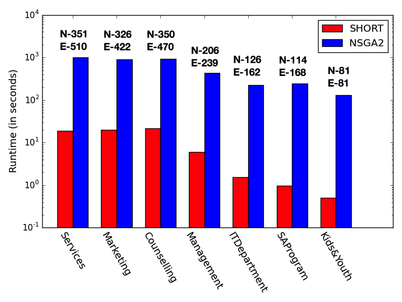
Figure 12: Runtimes for nsga2 compared to our approach. The number of nodes(N) and the edges(E) for each model is shown above the respective bar.

Fig. 12 shows the runtimes required to generate our results. Empirically, these runtimes fit the curve $\mathit{secs}=\mathit{nodes}^{2})$ with an $R^{2}=0.97$; i.e. SHORT’s runtimes are low-order polynomial. This is a significant result since in 1990, Bylander et al.warned that abductive search is NP-hard [19]; i.e. when exploring all options within an RE model, we should expect very slow runtimes. The pessimistic result has confirmed empirically by Menzies et al. [27], theoretically by Abdelbar et al. [20], and then again empirically by Ernst et al. [15].

It is insightful to compare SHORT’s runtimes against the forward and backwards analysis proposed by Horkoff and Yu [9]. They report times in the range of 7 to 300 seconds (which includes human time considering various choices)—which is approximately the same as the runtimes seen in Fig. 12. The advantage of backward and forward analysis is that user involvement increases user acceptance of the conclusions. The disadvantage is that those analysis methods do not comment on the robustness of the solution. Further, a forward and backwards analysis results in one sample of the model. A SHORT-style analysis, on the other hand, includes extensive “what-if” simulations. Charts like Fig. 10 not only offer solutions but also comments on:

• The stability of the selected decisions: see the red “IQR” line in that figure;

• The trade space across multiple decisions. Users can check a display of SHORT’s decision orderings (like Fig. 10) to decide for themselves when enough benefit has been obtained for enough cost.

To the best of our knowledge, forward and backward analysis has not been benchmarked against alternate techniques.

Our next results compare SHORT against a state-of-the-art multi-objective optimizer called NSGA-II [26]. This is a widely used genetic algorithm that uses a novel select operator to find the best “parents” to make the next generation. For both NSGA-II and SHORT, the goal is to maximize the coverage of goals and soft goals, while at the same time minimizing the sum of the costs of the decisions. Fig. 12 compares the median runtime for one run of NSGA-II and SHORT. Note that SHORT runs 2-3 orders of magnitude times faster.

In addition, NSGA-II returns just one solution, whereas SHORT reports what happens when an increasing number of decisions are imposed on a system (as done in Fig. 10). In order for NSGA-II to reason like SHORT, it would have to run hundreds of ‘what-if” studies. That is, NSGA-II’s runtime costs would be incurred hundreds of times.

To explain SHORT’s faster runtimes, we invoke the same reasoning used by Crawford and Baker, which we described in Section III-A. The RE models contain a small set of key variables that determine the rest. Hence, rigorously searching through all variable settings is not recommended since only a small number of those settings actually matter. Further, when the key decision variables are spread thinly over the entire model, it makes no sense to carefully explore many parts of the model (as done by NSGA-II) since much time will be wasted “walking” between the far-flung keys. For such models, if the reasoning gets stuck in one region, then the best thing to do is to leap at random to some distant part of the model (as done by SHORT’s random search).

Table III compares how objectives were covered in 20 repeated runs of NSGA-II and SHORT. Both approaches achieved remarkably similar coverage of goals—an effect that can be explained by our models having a small number of key variables which, if set the right way, control what can be achieved in the rest of the model.

Model	NSGA2	SHORT
Services	f1: 46.77 $\pm$ 0.0 f2: 65.22 $\pm$ 0.0	f1: 46.24 $\pm$ 0.0 f2: 65.22 $\pm$ 0.0
Marketing	f1: 32.47 $\pm$ 0.0 f2: 34.38 $\pm$ 0.0	f1: 32.47 $\pm$ 0.0 f2: 34.38 $\pm$ 0.0
Counselling	f1: 54.29 $\pm$ 1.41 f2: 44.83 $\pm$ 3.45	f1: 53.59 $\pm$ 2.76 f2: 44.83 $\pm$ 3.45
Management	f1: 44.63 $\pm$ 0.82 f2: 61.11 $\pm$ 2.78	f1: 42.98 $\pm$ 1.65 f2: 61.11 $\pm$ 2.78
ITDepartment	f1: 68.42 $\pm$ 2.63 f2: 69.57 $\pm$ 0.0	f1: 68.42 $\pm$ 2.63 f2: 73.91 $\pm$ 8.69
SAProgram	f1: 78.69 $\pm$ 1.64 f2: 66.67 $\pm$ 0.0	f1: 78.69 $\pm$ 1.64 f2: 66.67 $\pm$ 0.0
Kids&Youth	f1: 22.86 $\pm$ 0.0 f2: 100.0 $\pm$ 0.0	f1: 22.86 $\pm$ 0.0 f2: 100.0 $\pm$ 0.0

TABLE III: NSGA-II compared to our SHORT approach. Columns report Accuracy(Median $\pm$ IQR) of the objectives f1: Percentage of soft goals satisfied and f2: Percentage of goals satisfied.

VI Discussion

VI-A Can SHORT be applied to other modeling languages?

For our experiments, we used the models of Table I for two reasons. First, they are the largest requirements models we can access. Second, these models are representative of a large class of other requirements languages; i.e. those that can be compiled into what we call PCBN; i.e. Propositional assertions, where subsets of the propositions are augmented with Costs, Benefits, and Nogoods:

• The use of Costs was discussed, earlier in this paper in Section II.

• Benefits relate to a system’s high-level goals. For example, in Fig. 2, the lower leaves have zero benefit while the goals circled top-left have substantial benefit.

• Nogoods report what variable assignments are not allowed. For example, if a variable has mutually exclusive values, then it would be nogood for that variable to be given two different values.

Many modeling notations can be converted into PCBN. Menzies’ HT4 system included a domain general knowledge compiler that generated PCBN from (a) causal diagrams; (b) qualitative equations; a (c) frame-based knowledge representation; (d) compartmental models, and even (e) first-order systems (with finite-domains on the variables) [21].

Also, there are many recent examples of such knowledge compilation in the RE community. For example, any RE researcher using SAT solvers must write a knowledge compiler to convert their high-level notations into PCBN. Some of that research comes from within the i* community (e.g., [28]) and some from elsewhere. For example, see researchers using SAT solvers to explore van Lamsweerde’s goal graphs [29]; requirements for software product lines and feature models [30, 31], as well as other RE tools [32]. For a discussion on other RE models that can be compiled to propositions, see [5].

Last, we have some evidence that keys exist in non-PCBN models. The COCOMO tool suite is a system of numeric equations that offer predictions for software development time, effect, defects and risks. Menzies et al. [33] found that these systems have “keys” as we defined in Section II. In other work, we have documented key-like effects in procedural systems [34].

VI-B Why offer a new reasoning tool when others exist?

Many researchers use SAT solvers to find a solution within softgoals [35]. For example, Horkoff and Yu, in [36] discuss local propagation methods for reasoning backwards from goals or forwards from assertions across models like Fig. 2 (and sometimes, the Horkoff and Yu methods call SAT solvers as a sub-routine). Using SMT provers, these SAT solver methods can handle 1000s of elements (see the recent work of Nguyen et al. [37]).

Where SHORT differs from the above is that those methods find one solution while SHORT tries to build a trade space that summarizes the effects of decisions across all solutions. As discussed in Section III-A, an all solution approach is NP-hard and, prior to this paper, all reported attempts to address this problem have suffered from crippling runtimes that that prevented scale up  [11, 12]. SHORT is the first implementation we have found (in the last 20 years) that achieves low-order polynomial runtimes for large RE models.

That said, there could be advantages to combining SHORT with a forward or backwards analysis. Since SHORT is so fast, it could be run prior to a forward/backwards analysis in order to generate the trade space. Hence, stakeholders could then use it as a guide while debating trade-offs during the forward/backwards analysis. This could be one very promising future direction for this research.

VI-C What other goals beside minimizing costs can be used as an input and how can you identify them?

There are probably as many metrics as user goals in Requirements Engineering. For example, a) the functional and non-functional requirements [38] or b) the meta-requirements like cost, reused components, least defective, most different to existing system, etc. Methods for finding such engineering goals have been researched extensively in the qualitative software engineering literature, like summarizing opinions using card sort [39] or the knowledge acquisition literature [40]. SHORT is indifferent to the nature of the objectives the user aims to optimize, and can use any ordinal or continuous variables.

VI-D Threats to Validity

As with any empirical study, biases can affect the final results. Therefore, any conclusions made from this work must be considered with the following issues in mind:

Sampling bias threatens any experiment; i.e. what matters in (say) practitioner settings may not be true of our examples. The data sets used here comes from goal models taken from a repository and all but one were supplied by one individual. These were all from i* style models. That said, as argued above, the models we use here share many aspects with RE representations used by many other researchers. The Fig. 2 model was derived from consulting work done at the SEI with a large US government agency, and is ongoing. See [41] for more background.

Evaluation bias: This paper uses one measure of success, goal achievement and associated cost and benefit. Optimal solutions only consider inputs given, and may not reflect all the complexities of a given decision.

Construct Validity: The conclusions of this paper are about better processes for making decisions (specifically, do not waste time on all the numerous redundant issues). It would be a violation of construct validity to make another claim—that SHORT-guided decisions lead to better outcomes.

VI-E Future Work

SHORT can be expanded to work with quantitative goal modeling frameworks like KAOS [42].

The largest goal models used in this study has 351 nodes and 510 edges (refer to Fig. 1 and Table I), and from Fig. 12 we can see that this model can be reasoned in around 30 seconds compared to a classic optimization technique like NSGA2 (which takes around 900 seconds). Synthetic requirements engineering models can be generated by simulation [43] and can be used to demonstrate a greater scalability of SHORT.

SHORT provides a framework for visualizing the “keys” for an RE model but it requires the model to be encoded using the i* notation. This can be alleviated by defining a a uniform encoding scheme to support both qualitative and quantitative models. This scheme can then be used to power a Graphical User Interface tool to better aid stakeholders to develop models.

VII Conclusions

Confusing models can confuse stakeholders. One way to untangle complex models is to find the small number of key decisions that determine what can be done for the rest of the model.

Such keys are naturally occurring in RE models. For example, in eight large RE models sampled from the the i* community, we have found a small number of decisions (often, just 12%) was enough to to set the rest of the decisions. In stark contrast to much prior work [14, 15], finding these keys was very fast, using the randomized search methods employed in SHORT. Using these keys, SHORT is able to optimize RE models in time that was orders or magnitude faster than state-of-the-art optimizers. Further, the optimizations found by SHORT were competitive with those found by other, much slower, methods. Hence, our conclusions are that:

1. Keys can be found in numerous RE models;

2. Keys are easy to find;

3. It is very useful to apply keys for reasoning about RE models.

Technical Appendix

Reproduction Package

All our tools and models are available on-line at https://goo.gl/gvxeaH. While some aspects of our approach are specific to goal models, the general SHORT method could be applied to a wide range of models.

Graph Smoothing

To smooth out the charts generated in SHORT (e.g. Figure 10), we use the Scott-Knott procedure recommended by [44]. This technique recursively bi-clusters a sorted set of numbers. If any two clusters are statistically indistinguishable, Scott-Knott reports them both as one line. E.g. for lists $l,m,n$ of size $ls,ms,ns$ where $l=m\cup n$, Scott-Knott divides the sequence at the break that maximizes:

$$E(\Delta)=\frac{ms}{ls}abs(m.\mu-l.\mu)^{2}+\frac{ns}{ls}abs(n.\mu-l.\mu)^{2}$$

Scott-Knott then applies some statistical hypothesis test $H$ to check if $m,n$ are significantly different. If so, Scott-Knott then recurses on each division. For this study, our hypothesis test $H$ was a conjunction of the A12 effect size test (endorsed by [45]) and non-parametric bootstrap sampling [46]; i.e. our Scott-Knott divided the data if both bootstrapping and an effect size test agreed that the division was statistically significant (99% confidence) and not a “small” effect ($A12\geq 0.6$).

References

- [1] L. Chung, J. Mylopoulos, and B. A. Nixon, “Representing and Using Nonfunctional Requirements: A Process-Oriented Approach,” IEEE Transactions on Software Engineering, vol. 18, pp. 483–497, 1992.
- [2] A. van Lamsweerde, “Goal-Oriented Requirements Engineering: A Guided Tour,” in Proceedings of the IEEE Joint International Conference on Requirements Engineering, Toronto, 2001, pp. 249–263.
- [3] D. Amyot, S. Ghanavati, J. Horkoff, G. Mussbacher, L. Peyton, and E. S. K. Yu, “Evaluating Goal Models within the Goal-oriented Requirement Language,” International Journal of Intelligent Systems, vol. 25, no. 8, pp. 841–877, 2010.
- [4] H. Kaiya, H. Horai, and M. Saeki, “AGORA: Attributed Goal-Oriented Requirements Analysis Method,” in Proceedings of the IEEE Joint International Conference on Requirements Engineering, Essen, Germany, 2002, pp. 13–22.
- [5] I. J. Jureta, A. Borgida, N. Ernst, and J. Mylopoulos, “Techne: Towards a New Generation of Requirements Modeling Languages with Goals, Preferences, and Inconsistency Handling,” in Proceedings of the IEEE Joint International Conference on Requirements Engineering, Sydney, Australia, 2010, pp. 115–124.
- [6] E. S. K. Yu, “Towards modelling and reasoning support for early-phase requirements engineering,” in Proceedings of the IEEE Joint International Conference on Requirements Engineering, Annapolis, Maryland, 1997, pp. 226–235.
- [7] H. A. Simon, The Sciences of the Artificial. MIT Press, 1996.
- [8] T. P. Moran and J. M. J. M. Carroll, Design rationale : concepts, techniques, and use, ser. Computers, cognition, and work. L. Erlbaum, 1996.
- [9] J. Horkoff and E. Yu, “Interactive goal model analysis for early requirements engineering,” Requirements Engineering, vol. 21, no. 1, pp. 29–61, 2016.
- [10] R. Williams, C. P. Gomes, and B. Selman, “Backdoors to typical case complexity,” in Proceedings of the International Joint Conference on Artificial Intelligence, 2003.
- [11] S. Amarel, “Program synthesis as a theory formation task: problem representations and solution methods,” in Machine Learning: An Artificial Intelligence Approach. Morgan Kaufmann, 1986.
- [12] J. M. Crawford and A. B. Baker, “Experimental results on the application of satisfiability algorithms to scheduling problems,” in Proceedings of the Twelfth National Conference on Artificial Intelligence (Vol. 2), Menlo Park, CA, USA, 1994, pp. 1092–1097.
- [13] R. Kohavi and G. H. John, “Wrappers for feature subset selection,” Artif. Intell., vol. 97, no. 1-2, pp. 273–324, Dec. 1997.
- [14] T. Menzies, “Applications of abduction: knowledge-level modelling,” International journal of human-computer studies, vol. 45, no. 3, pp. 305–335, 1996.
- [15] N. Ernst, A. Borgida, J. Mylopoulos, and I. J. Jureta, “Agile Requirements Evolution via Paraconsistent Reasoning,” in International Conference on Advanced Informations Systems Engineering, Jun. 2012, pp. 1–16.
- [16] B. Nuseibeh, “To be and not to be: On managing inconsistency in software development,” in Proceedings of the 8th International Workshop on Software Specification and Design. IEEE Computer Society, 1996, p. 164.
- [17] D. Poole, “Who chooses the assumptions?” in The Management of Uncertainty in AI, IJCAI’93, 1993.
- [18] J. De Kleer, “An assumption-based tms,” Artificial intelligence, vol. 28, no. 2, pp. 127–162, 1986.
- [19] T. Bylander, D. Allemang, M. C. Tanner, and J. R. Josephson, “The computational complexity of abduction,” Artificial Intelligence, vol. 49, no. 1-3, pp. 25–60, 1991.
- [20] A. M. Abdelbar, “Approximating cost-based abduction is np-hard,” Artif. Intell., vol. 159, no. 1-2, pp. 231–239, Nov. 2004.
- [21] T. Menzies, “Applications of abduction: knowledge-level modelling,” International Journal of Human-Computer Studies, pp. 305–335, 1996.
- [22] E. Zitzler and S. Künzli, Indicator-Based Selection in Multiobjective Search. Berlin, Heidelberg: Springer Berlin Heidelberg, 2004, pp. 832–842.
- [23] R. Storn and K. Price, “Differential evolution–a simple and efficient heuristic for global optimization over continuous spaces,” Journal of global optimization, vol. 11, no. 4, pp. 341–359, 1997.
- [24] W. Fu, T. Menzies, and X. Shen, “Tuning for software analytics: Is it really necessary?” Information and Software Technology, vol. 76, pp. 135–146, 2016.
- [25] J. Krall, T. Menzies, and M. Davies, “Gale: Geometric active learning for search-based software engineering,” IEEE Transactions on Software Engineering, vol. 41, no. 10, pp. 1001–1018, 2015.
- [26] K. Deb, A. Pratap, S. Agarwal, and T. Meyarivan, “A fast and elitist multiobjective genetic algorithm: NSGA-II,” Trans. Evol. Comp, vol. 6, no. 2, pp. 182–197, Apr. 2002.
- [27] T. Menzies, “Applications of abduction: knowledge-level modelling,” International Journal of Human-Computer Studies, vol. 45, no. 3, pp. 305 – 335, 1996.
- [28] Y. Wang and J. Mylopoulos, “Self-repair through reconfiguration: A requirements engineering approach,” in Proceedings of the IEEE/ACM International Conference on Automated Software Engineering. IEEE Computer Society, 2009, pp. 257–268.
- [29] A. van Lamsweerde, “Requirements engineering: from craft to discipline,” in Proceedings of the 16th ACM SIGSOFT International Symposium on Foundations of software engineering. ACM, 2008, pp. 238–249.
- [30] A. Classen, P. Heymans, and P.-Y. Schobbens, “What’s in a feature: A requirements engineering perspective,” in International Conference on Fundamental Approaches to Software Engineering. Springer, 2008, pp. 16–30.
- [31] M. Mendonca, A. Wąsowski, and K. Czarnecki, “Sat-based analysis of feature models is easy,” in Proceedings of the International Software Product Line Conference, 2009, pp. 231–240.
- [32] D. Benavides, S. Segura, P. Trinidad, and A. R. Cortés, “Fama: Tooling a framework for the automated analysis of feature models.” VaMoS, vol. 2007, p. 01, 2007.
- [33] T. Menzies, O. Elrawas, J. Hihn, M. Feather, R. Madachy, and B. Boehm, “The business case for automated software engineering,” in Proceedings of the IEEE/ACM International Conference on Automated Software Engineering, 2007, pp. 303–312.
- [34] T. Menzies, D. Owen, and J. Richardson, “The strangest thing about software,” IEEE Computer, pp. 54–60, 2007.
- [35] R. Sebastiani, P. Giorgini, and J. Mylopoulos, “Simple and Minimum-Cost Satisfiability for Goal Models,” in Proceedings of the International Conference on Advanced Information Systems Engineering, Riga, Latvia, 2004, pp. 20–35.
- [36] J. Horkoff and E. Yu, “Comparison and evaluation of goal-oriented satisfaction analysis techniques,” Requirements Engineering, vol. 18, no. 3, pp. 199–222, 2013.
- [37] C. M. Nguyen, R. Sebastiani, P. Giorgini, and J. Mylopoulos, “Multi-objective reasoning with constrained goal models,” Requirements Engineering, pp. 1–37, 2016.
- [38] L. Chung, B. A. Nixon, E. Yu, and J. Mylopoulos, Non-functional requirements in software engineering. Springer Science & Business Media, 2012, vol. 5.
- [39] X. Yuan, N. Sa, G. Begany, and H. Yang, “What users prefer and why: a user study on effective presentation styles of opinion summarization,” in Human-Computer Interaction. Springer, 2015, pp. 249–264.
- [40] A. Guzzi, A. Bacchelli, M. Lanza, M. Pinzger, and A. Van Deursen, “Communication in open source software development mailing lists,” in IEEE Working Conference on Mining Software Repositories, 2013, pp. 277–286.
- [41] N. A. Ernst, M. Popeck, F. Bachmann, and P. Donohoe, “Creating software modernization roadmaps: The architecture options workshop,” in 13th Working IEEE/IFIP Conference on Software Architecture, Venezia, 2016.
- [42] A. Van Lamsweerde, Requirements engineering: From system goals to UML models to software. Chichester, UK: John Wiley & Sons, 2009, vol. 10.
- [43] C. Seybold, S. Meier, and M. Glinz, “Evolution of requirements models by simulation,” in Software Evolution, 2004. Proceedings. 7th International Workshop on Principles of. IEEE, 2004, pp. 43–48.
- [44] N. Mittas and L. Angelis, “Ranking and clustering software cost estimation models through a multiple comparisons algorithm,” IEEE Transactions on Software Engineering, vol. 39, no. 4, pp. 537–551, 2013.
- [45] A. Arcuri and L. Briand, “A practical guide for using statistical tests to assess randomized algorithms in software engineering,” in Proceedings of the ACM/IEEE International Conference on Software Engineering. IEEE, 2011, pp. 1–10.
- [46] B. Efron and R. J. Tibshirani, An introduction to the bootstrap, ser. Mono. Stat. Appl. Probab. London: Chapman and Hall, 1994.