A simple mathematical model
inspired by the Purkinje cells:
from delayed travelling waves
to fractional diffusion

Abstract.

Recently, several experiments have demonstrated the existence of fractional diffusion in the neuronal transmission occurring in the Purkinje cells, whose malfunctioning is known to be related to the lack of voluntary coordination and the appearance of tremors.

Also, a classical mathematical feature is that (fractional) parabolic equations possess smoothing effects, in contrast with the case of hyperbolic equations, which typically exhibit shocks and discontinuities.

In this paper, we show how a simple toy-model of a highly ramified structure, somehow inspired by that of the Purkinje cells, may produce a fractional diffusion via the superposition of travelling waves that solve a hyperbolic equation.

This could suggest that the high ramification of the Purkinje cells might have provided an evolutionary advantage of “smoothing” the transmission of signals and avoiding shock propagations (at the price of slowing a bit such transmission). Although an experimental confirmation of the possibility of such evolutionary advantage goes well beyond the goals of this paper, we think that it is intriguing, as a mathematical counterpart, to consider the time fractional diffusion as arising from the superposition of delayed travelling waves in highly ramified transmission media.

The case of a travelling concave parabola with sufficiently small curvature is explicitly computed.

The new link that we propose between time fractional diffusion and hyperbolic equation also provides a novelty with respect to the usual paradigm relating time fractional diffusion with parabolic equations in the limit.

This paper is written in such a way as to be of interest to both biologists and mathematician alike. In order to accomplish this aim, both complete explanations of the objects considered and detailed lists of references are provided.

1. Introduction

Anomalous diffusion is becoming increasingly more popular to describe complex systems, in which the conventional diffusion described by Brownian motion is inadequate. Among the different types of anomalous diffusion, a special role is played by fractional diffusion, both in time and space variables. Recent experiments (see [4, 5, 9, 20, 21, 24, 25, 26, 33, 34, 35, 36, 38, 39, 44, 46, 47, 51] and the references therein) confirmed the evidence of fractional diffusions in many systems of biological interest, though a complete understanding of all the phenomena involved is still to be found, and many theoretical aspects of fractional diffusion still needs to be further investigated.

This article is devoted to the derivation of a time fractional diffusion equation from a “basic building-block”, that is given by a set of classical travelling waves. The model that we investigate is inspired by the Purkinje cells, in which the complex ramification of the medium produces a selected delay in the transmission of the waves.

From the mathematical point of view, the superposition of these delays produces a fractional operator. In this way, a new link between a time fractional diffusion equation (a parabolic equation) and a classical wave equation (a hyperbolic one) will be introduced. In spite of the fact that these two types of equations present qualitatively very different properties, the highly ramified structure of the transmission network allows us to reduce one equation to the other.

From the biological point of view, the results described in this article may give a possible explanation of the causes of some malfunction of the Purkinje cells.

1.1. Aims and results

The goal of this note is to provide a mathematical derivation from basic principle of the fractional diffusion equation

$$D^{s}_{t}u=\kappa\,c^{s}\,L^{2-s}\,\partial^{2}_{x}u$$ (1.1)

in view of some recent experiments on the Purkinje cells (and, in general, on neural structures), which seem to exhibit this type of nonlocal diffusion. In equation (1.1), the function $u$ plays the role of a diffusive substance (the concrete substance depending on the particular type of diffusion considered in different specific situations), $\kappa$ is an adimensional normalization constant, and $c$ and $L$ are fixed quantities (representing, respectively, the velocity of propagation of an elementary signal and the length of the propagation device).

Moreover, the notation $D^{s}_{t}$ stands for a time fractional derivative, that, for definiteness, we take here in the sense of Caputo. Namely, we recall the notion of Caputo fractional derivative of order $s\in(0,1)$ (see [12]), i.e. we set

$$D^{s}_{t}u(t):=\frac{1}{\Gamma(1-s)}\int_{0}^{t}\frac{\dot{u}(\tau)}{(t-\tau)^{s}}\,d\tau,$$ (1.2)

where $\Gamma$ is the Euler’s Gamma-function (which, for a fixed $s\in(0,1)$, also plays in (1.2) just the role of a normalizing factor).

Equations such as (1.1) have recently appeared in connection to several experimental data and theoretical considerations related to the diffusion in the Purkinje cells: compare, in particular, formula (1.1) here with the first formula in display in [34] and see also [46, 45].

To the best of our knowledge, the scientific literature has presented several deep and interesting descriptions of the time fractional diffusion in (1.1) also in connection with neuronal biology, see e.g. the discussion related to formulas (8.3), (8.12) and (8.13) in [35], but no attempt has been made till now to derive equation (1.1) from “basic principles” in a (possibly highly simplified) toy-model somehow related to neurons.

Our goal in this paper is to try to fill this gap in the literature, since we believe that derivations from basic principles and from simpler equations have several cultural and practical benefits, such as clarifying a difficult but important research subject, enlarging the community of researchers working on a field, providing connections with different subjects and leading to a deeper and broader understanding of the phenomena. Of course, in this type of derivation processes some dramatic simplification has sometimes to be expected, in order to reduce the arguments to the core whenever possible, and, in this sense, the situation that we present in this paper should not be intended as a “full explanation” of the functioning of the complex neural networks, but only as a simplified (though, in our opinion, sufficiently “realistic” and with concrete scientific value) model, related to, or at least inspired by, a simplified version of neural network.

Also, differently from the classical literature, our aim is not to relate fractional diffusion with the standard one (which is formally obtained in the limit as $s\nearrow 1$), but rather to see fractional diffusion as a superposition of hyperbolic equations with a delay. In our setting, such delay is caused by the ramification of the mathematical structure on which the hyperbolic equation takes place.

The construction of this ramified medium is inspired by the structure of the Purkinje cells, which are a class of neurons located in the cerebellum, with a highly ramified structure, whose activity is of crucial importance for the coordination of complex motions.

As a matter of fact, the malfunctioning of the Purkinje cells may lead (among other symptoms) to ataxia (i.e., lack of voluntary coordination), tremors and hyperreactivity, see e.g. [9, 36] and the references therein.

Thus, one of the roles of the ramified structure of the Purkinje cells seems to be that of somehow “smoothing out” sharp impulses. A mathematical counterpart of this phenomenon can be seen by comparing the smoothing effects of the heat equation with the shocks typical of hyperbolic equations (see e.g. [22]). Motivated by these considerations, we provide a toy-model in which the fractional diffusion in (1.1) comes from the superposition of travelling waves. In a sense, the highly ramified structure of the diffusion device (in the appropriate space/time scale limit) provides, at the end of the structure, an averaged superposition of travelling waves with a nonlinear delay which, in turn, transforms the hyperbolic equation of a single travelling wave into a nonlocal (in time) diffusion of the averaged function as in (1.1), thus providing a regularizing effect on the solution.

This construction suggests the possibility that the fractional diffusion experimentally found in neurons could be related to the possibility of smoothing irregular signals, so to make the coordination of the movements less subject to shocks and discontinuities. In this sense, it is intriguing to wonder whether the regularizing effects of fractional parabolic equations (when compared to hyperbolic equations) could be seen as a mathematical counterpart of an evolutionary advantage of the high ramification of the Purkinje cells, with the benefit of smoothing the transmission of the signals and perhaps favoring, at least indirectly, a general coordination of the organism.

Roughly speaking, the mathematical effect of highly ramified arbors in the transmission of signals may be thought as producing selected and appropriate delays in the signal transmission. The appropriately tuned superposition of these delays has the combined effect to somehow “average” the propagation of the signal, by producing a situation similar to those of fractional diffusion, in which the speed at which diffusion takes place is “anomalous”, i.e. it does not coincide with the classical one prescribed by the Gaussian function. Such a delay behavior, when finely tuned, might somehow contribute to coordinate these signals, rather than just retarding the whole transmission, since the regularizing features of fractional parabolic equations smooth out the data (differently from the case of standard transmissions through hyperbolic equations).

1.2. Fractional diffusion under different perspectives

The contemporary literature in mathematical biology has considered anomalous diffusion of fractional type in several experiments and under different points of view. Several recent works considered fractional diffusion in view of the so-called “input-output analysis”: namely, accurate measurements are performed to discover underlying biological mechanisms, often related to linear equations. See in particular [50] for the point of view of physiology on the power law distributions arising in the outputs of several receptors. In this, a classical approach of [49] is that of considering powers of time as linear superpositions of many different exponential decays, in conformity with the definition of the Euler’s Gamma-function, see in particular formula (1) in [50] and the references therein (a Gamma-function approach is also useful to link space fractional diffusion and classical heat semigroups, see e.g. formulas (2.11) and (2.12) of [11]).

The approach of [49, 50] has also been exploited in the analysis of cells and tissues, see e.g. formula (2.2) in [33]. Also, in [33] fractional calculus is used to study a tissue-electrode interface between cardiac muscle cells. Related methods have also been exploited in [4] for the analysis of the vestibulo-ocular system.

In [18], the time fractional derivative is used to model several phenomena. First, fractional derivatives of order $s\in(0,1)$ are seen as natural interpolations between elasticity laws of Hooke type (in which the displacement corresponds to a derivative of order $s=0$) and viscosity theories of Newton type (in which the velocity corresponds to a derivative of order $s=1$): with this respect, fractional derivatives turn out to provide an interesting model for viscoelastic materials. Then, some biological models are discussed in [18], with special attention to protein adsorption kinetics. Finally, cognitive processes are also taken into account in [18], showing a fit with classic memorizing testing data by Hermann Ebbinghaus which date back to 1885. As a technical remark, we observe that in [18] the Riemann-Liouville derivative is taken as basic model for time fractional diffusion, instead of the Caputo derivative that we consider here (compare formula (2) in [18] with (1.2) here): nevertheless the two fractional derivatives are closely related, up to a term involving the initial condition, see e.g. formula (4) in [6].

A recent review of many different results of fractional calculus in bioscience and engineering, with special emphasis in respiratory tissues and drug diffusion is given in [27]. See in particular Section 4.3 in [27] for a discussion on the many applications of fractional calculus in neuroscience.

Though our paper mainly focuses on one single example, namely that of the transmission problem in a highly ramified network, we believe that our approach is general enough to be applicable also to other models (see e.g. Section 4.4 in [1]).

1.3. Topics and methods

In our analysis, the mathematical methods exploited are all of elementary nature (integration by parts, change of variable, superposition principle, integration theory, basic PDE), all the ansatz and approximation assumptions are clearly stated step by step, the biological motivations are explained without assuming major prerequisites and providing quite exhaustive lists of classical and contemporary references, and we also indulge in explanations and clarifications, therefore the paper is easily usable by a wide group of interested researchers. Our goal here is not to give a complete explanation of the rich phenomena encoded by the complex structure of the Purkinje cells; nevertheless, we believe that the mathematical approach that we present here is useful to better understand some specific neuronal features. Moreover, the new connection between fractional diffusion and hyperbolic equations may lead to a better understanding of the smoothing effects for travelling signals that are favored by the highly ramified neuronal structures.

Furthermore, though a clear understanding of the time fractional diffusion in real world phenomena will require combined efforts from different perspectives (e.g. with synergic approaches from biology, chemistry, physics, etc.), we hope that the mathematical insight presented here can better motivate the interest of fractional diffusion among the mathematical community, serve as a foundation ground for scientists with different backgrounds and suggest new connections between very different types of evolution equations, such as hyperbolic and (fractional) parabolic ones, which are made possible by the highly complex structures of the media. Also, we believe that a mathematical model easy to handle may provide some initial insight (to be enhanced by quantitative and more sophisticated studies) about the level at which fractional diffusion arises in many natural phenomena, also trying to give information on the scales involved and on the basic causes of these features.

1.4. Organization of the paper

The rest of this paper is organized as follows. In Section 2 we recall some basic facts about the Caputo derivative and the related time fractional diffusion. In particular, a simple integration by parts procedure, combined with an appropriate change of variables, relates the Caputo derivative to the superpositions of delayed classical second derivatives.

Then, in Section 3, we will introduce a highly ramified mathematical structure, inspired by the neuronal spikes, and study the transmission of a hyperbolic travelling wave along such complex medium. We will see that the structure of the medium produces the superposition of delayed travelling waves which, at the end of the transmission device, in average and in the appropriate limit sense, can be related to the fractional derivative and produce the time fractional diffusion equation in (1.1).

In the computations needed for this scope, an ancillary limit formula is stated, whose proof is given, for the facility of the reader, in Section 4.

The conclusions of this paper are then summarized in Section 5.

2. Integration by parts in the Caputo derivative

The notion of fractional diffusion provides at the moment an intense topic of research, both for its very challenging theoretical difficulties and in view of concrete applications in biology, physics and finance (see e.g. [11] for several explicit discussions and motivations). In general, fractional diffusion presents several phenomena in common with the classical diffusion arising from Gaussian processes and Brownian motions, such as the regularizing effects with respect to initial data: in this sense, see in particular [30] for a regularity theory in Lebesgue spaces, and also [53] for a regularity theory in Hölder spaces (see also page 103 in [54] for a general discussion about the relation between “abstract Volterra equations” and the time fractional diffusion). For higher regularity in time, see also Section 5 of [2], and for related results see [3].

Furthermore, important and often unexpected differences between classical and fractional diffusion arise: for instance, solutions of fractional equations can locally approximate any given function, in sharp contrast with the classical case, see [16, 10, 17].

The monograph [15] also provides extensive and throughout discussions about fractional derivatives in time also in view of many applications. See also [37] for an approach to different types of time fractional derivatives from the perspectives of stochastic processes with long rests.

Here, we recall some basic facts on the fractional Caputo derivative in (1.2) and perform some preliminary computations which will be used in the forthcoming sections. To start with, for notational convenience, we scale the constant in (1.2) and we integrate by parts, by obtaining that

$$\begin{split}\partial^{s}_{t}u(t)\,&:=(2-s)\,(1-s)\,\Gamma(1-s)\,D^{s}_{t}u(t)\\ &=(2-s)\,(1-s)\,\int_{0}^{t}\frac{\dot{u}(\tau)}{(t-\tau)^{s}}\,d\tau\\ &=-(2-s)\,\int_{0}^{t}\frac{\partial}{\partial\tau}\big{(}(t-\tau)^{1-s}\,\dot{u}(\tau)\big{)}\,d\tau+(2-s)\,\int_{0}^{t}(t-\tau)^{1-s}\,\ddot{u}(\tau)\,d\tau\\ &=(2-s)\,t^{1-s}\,\dot{u}(0)+(2-s)\,\int_{0}^{t}(t-\tau)^{1-s}\,\ddot{u}(\tau)\,d\tau.\end{split}$$ (2.1)

Using the substitution $\vartheta:=(t-\tau)^{2-s}$, we thus obtain

$$\partial^{s}_{t}u(t)=(2-s)\,t^{1-s}\,\dot{u}(0)+\int_{0}^{t^{2-s}}\ddot{u}(t-\vartheta^{\beta})\,d\vartheta,$$ (2.2)

where

$$\beta:=\frac{1}{2-s}\in\left(\frac{1}{2},1\right).$$ (2.3)

As a matter of fact, the computations leading to (2.1) are merely formal, since we are tacitly assuming here that $u$ is smooth and has a well-defined second time derivative. Our goal is now to interpret (2.2) as a superposition of delayed effects caused by the ramified structure of the transmission medium, which is somehow inspired by the structure of the Purkinje cells (in neuronal transmissions, other types of delays leading to fractional diffusion may be caused by obstacles and bindings, see [48]).

3. A simple model towards the fractional diffusion in the Purkinje cells

In this section, we present a transmission media built by a highly ramified structure. Such mathematical model is qualitatively inspired by the dendritic arbor of the Purkinje cells. We will consider the transmission along this medium, as prescribed by the classical wave equation. The ramifications of the medium will cause the delay of some signals, whose superposition at the end of the structure will be related to the fractional derivative.

In this setting, the superposition of travelling waves with a suitably tuned delay will produce a time fractional diffusion in the formal limit, thus providing a new bridge between equations of very different kind (i.e. hyperbolic and fractional parabolic) with the aim of encoding some of the features observed by the experiments in neuronal dendrites, such as the time fractional diffusion in the spikes of the Purkinje cells.

In the classical transmission line analysis (see e.g. pages 5–14 in [29]) the variation in space of the potential is related, via inductance, to the variation in time of the intensity of current; on the other hand, the variation in space of the intensity of current is related, via capacitance, to the variation in time of the potential. The combination of these equations naturally lead to the wave equation (for a derivation of the wave equation directly from Maxwell’s equations see e.g. (3.14) and (3.15) in [7]). For models presenting wave equations in cylindrical neurons, see e.g. formulas (6.20) and (6.21) in [43], and also [5, 25, 28, 32].

We remark that the analysis of travelling waves in neurons is a classical and active topic of study in itself, see e.g. [21, 20, 42, 38, 13]. See also [51] for other mathematical models related to diffusion in neurons based on Monte Carlo methods.

3.1. Model of the ramified structure

The model of the ramified medium that we take into account is a very basic simplification inspired by a branch of the Purkinje cell and goes as follows.

We let $N\in\mathbb{N}$ (to be taken large in the sequel) and

$$b_{N}:=\sum_{1\leqslant k\leqslant N}\frac{1}{{k}^{\alpha}},$$ (3.1)

with

$$\alpha:=\frac{1-s}{2-s}=1-\beta\in\left(0,\frac{1}{2}\right)$$ (3.2)

and $\beta$ as in (2.3). We let also

$$\begin{split}&\ell_{k}:=\frac{L}{k^{\alpha}b_{N}}\\ {\mbox{and }}\quad&\lambda_{k}:=\sum_{1\leqslant j\leqslant k}\ell_{j}.\end{split}$$ (3.3)

We consider a set of $N$ planar curves, with one common endpoint and the other endpoint lying on a common straight line. These curves will be denoted by $S_{1},\dots,S_{N}$. The length of $S_{1}$ is set to be $L>0$. The length of $S_{2}$ is set to be $L+\ell_{1}$. Iteratively, the length of $S_{k}$, for each $k\in\{2,\dots,N\}$ is set to be equal to

$$L+\ell_{1}+\dots+\ell_{k-1}=L+\lambda_{k-1}.$$

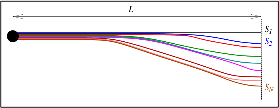
Figure 3.1. The ramified media along which we study the delayed transmission (an exemplifying, not quantitative, picture).

See Figure 3.1 for an exemplifying representation of such medium. Of course, the reader may compare this picture and the classical drawing by S. Ramón y Cajal, see e.g. [52] as well as the many realistic pictures available nowadays, to appreciate the motivation related to the Purkinje cell – though of course we do not aim to a full understanding of the Purkinje cell by the very simplified model described here. We stress, in particular, that when we refer to concepts like “horizontal”, “left” or “right” we are clearly making no reference to concrete special directions in the cerebellum, but rather we are referring to the toy-model drawn in Figure 3.1: in any case, as it will be apparent in the computation, these directions play no role in our derivation, what counts is only the fact that the ramification produces branches of different lengths or, better to say, just the fact that the speed to travel to the end of a branch depends on the branch itself. Also, Figure 3.1 can be immersed in a more complicated neural network and we only focus on a “single” ramified system to keep the discussion as simple as possible (in practice, of course, the response to an organism depends on the signal transmissions in many cells and not just one).

See also [23, 41] and the references therein for accurate descriptions of dendritic arbors.

Of course, different scalings and different parameters in the model presented lead to quantitatively different versions of fractional diffusions, which may be seen as the mathematical counterpart of the quantitative differences explored in [47] in view of the different densities of dendritic spines. See also [8] for an accurate analysis of anomalous diffusion in fractal media. Of course, a detailed description of the geometry of the dendritic spines also in terms of density and statistics of the ramification may produce a better understanding of the neuronal diffusion and inspire quantitatively more accurate models. In addition, it would be very interesting to further investigate these questions and related problems in the light of the theory of wave propagation in networks (see e.g. [14] and the references therein, where however Dirichlet or control conditions are usually assumed on the vertices of the graphs, also in relation with vibrating strings with joined extrema).

3.2. Travelling waves in the ramified medium and their effect at the right end of the structure

We will now take into account a travelling wave in the structure depicted in Figure 3.1, and compute the averaged effect of the delay induced by the ramification of the medium.

From the biological point of view, we think it is worth justifying our choice of considering hyperbolic equations as “building blocks” of our derivation procedure. Indeed, some of the equations proposed to model neuronal diffusion, such as the Hodgkin-Huxley equation, are of parabolic, rather then hyperbolic type. Nevertheless, we chose not to consider the Hodgkin-Huxley equation as the basis of our model, for several reasons. First of all, the Hodgkin-Huxley equation [26] is a rather complicated model and, at least from an “aesthetic” perspective, does not seem to be suitable as a “basic principle” from which one derives a time fractional process. More importantly, there are in the literature some non-thermodynamical theories that suggest (and some experiments support) that mechanical waves accompany action potentials, see [19, 24]. Furthermore, it is known that some reaction-diffusion processes can produce solitons and travelling waves, see [40].

For these reasons, we thought it was intriguing, and also sufficiently realistic, to take the wave equation as the basic to deduce a time fractional equation in our simplified setting.

Thus, the idea is to consider a travelling wave (say, from left to right) in such medium, whose “natural speed” is given by $c>0$, that is a (smooth) function

$$f=f(x,t)=f_{o}\left({\frac{x-ct}{L}}\right)$$ (3.4)

satisfying

$$\partial^{2}_{t}f(x,t)=c^{2}\partial^{2}_{x}f(x,t)={\frac{c^{2}}{L^{2}}f_{o}^{\prime\prime}\left({\frac{x-ct}{L}}\right)},$$ (3.5)

and analyze (for large $N$) its effect on the right end of the structure, which we will denote by $u$.

In our toy-model, the function $u$ at the right end of the structure represents, somehow, the relevant information that the left end of the structure “sends” to the organism: in this sense, we think it is natural to consider such information at the right end of the structure as the superposition of the information sent in each of the branches which connect the left end to the right end. In view of this, we will see that $u$ is the superposition of a series of $f$’s, shifted by a nonlinear delay (a precise formula will be given in (3.13) below).

Roughly speaking, the effect of any travelling function $f$ on the right end of the structure may be seen as the superposition of the $1/N$-contributions of $f$ along each of the ramifications $S_{k}$, for $k\in\{1,\dots,N\}$. Each of these contributions will be denoted by $f_{k}$. We drop the dependence on $x$ for the sake of simplicity and we assume that $f_{1}(t)=\frac{f(t)}{N}$, namely the contributions are “equally spread” on the ramifications. Also, we observe that the length travelled by the function $f_{2}$ is equal to the one travelled by $f_{1}$ (which is in turn given by $L$) plus the length of the additional quantity $\ell_{1}$. This causes a phase delay of $f_{2}$ with respect to $f_{1}$ of size $c^{-1}\ell_{1}$. Hence

$$f_{2}(t)=f_{1}(t-c^{-1}\ell_{1}).$$

Iteratively, for each $k\in\{2,\dots,N\}$, the length travelled by the function $f_{k}$ is equal to the one travelled by $f_{k-1}$ plus the length of the additional quantity $\ell_{k-1}$. This causes a phase delay of $f_{k}$ with respect to $f_{k-1}$ of size $c^{-1}\ell_{k-1}$. Hence

$$f_{k}(t)=f_{k-1}(t-c^{-1}\ell_{k-1}).$$

Accordingly

$$f_{k}(t)=f_{k-1}(t-c^{-1}\ell_{k-1})=f_{k-2}(t-c^{-1}\ell_{k-1}-c^{-1}\ell_{k-2})$$

$$\qquad=\dots=f_{k-i}(t-c^{-1}\ell_{k-1}-c^{-1}\ell_{k-2}-\dots-c^{-1}\ell_{k-i})$$

$$\qquad=\dots=f_{1}(t-c^{-1}\ell_{k-1}-c^{-1}\ell_{k-2}-\dots-c^{-1}\ell_{1})=f_{1}(t-c^{-1}\lambda_{k-1})$$

$$\qquad=\frac{f(t-c^{-1}\lambda_{k-1})}{N}.$$

Hence, the total contribution of a travelling function $f$ on the right side of the structure is taken to be

$$\sum_{1\leqslant k\leqslant N}f_{k}(t)=\frac{1}{N}\sum_{1\leqslant k\leqslant N}f(t-c^{-1}\lambda_{k-1}).$$ (3.6)

We set

$$\begin{split}&\eta_{k,N}:=L\,\left(\frac{k}{N}\right)^{1-\alpha}-\lambda_{k-1}\\ {\mbox{and }}\;&\epsilon_{N}:=\sup_{k\in\{1,\dots,N\}}|\eta_{k,N}|\end{split}$$ (3.7)

and it can be shown that

$$\lim_{N\to+\infty}\epsilon_{N}=0.$$ (3.8)

Not to interrupt this calculation, we postpone the proof of (3.8) to Section 4.

Now, in view of (3.6) and (3.8), the total contribution of a smooth travelling function $f$ on the right side of the structure becomes

$$\begin{split}&\frac{1}{N}\sum_{1\leqslant k\leqslant N}f\left(t-c^{-1}L\,\left(\frac{k}{N}\right)^{1-\alpha}+c^{-1}\,\eta_{k,N}\right)\\ =\;&\frac{1}{N}\sum_{1\leqslant k\leqslant N}\left[f\left(t-c^{-1}L\,\left(\frac{k}{N}\right)^{1-\alpha}\right)+O(c^{-1}\,\epsilon_{N})\right]\\ =\;&\frac{1}{N}\sum_{1\leqslant k\leqslant N}f\left(t-c^{-1}L\,\left(\frac{k}{N}\right)^{1-\alpha}\right)+O(c^{-1}\,\epsilon_{N}).\end{split}$$ (3.9)

We now recognize a Riemann sum, namely we have that

$$\begin{split}&\lim_{N\to+\infty}\frac{1}{N}\sum_{1\leqslant k\leqslant N}f\left(t-c^{-1}L\,\left(\frac{k}{N}\right)^{1-\alpha}\right)\\ =\;&\int_{0}^{1}f\left(t-c^{-1}\,L\,\zeta^{1-\alpha}\right)\,d\zeta.\end{split}$$ (3.10)

For clarity, we now distinguish between the time variable $t$ and the natural time scale of the problem, which will be denoted by $T$. While $t$ is a free coordinate and it is one of the arguments of the functions under considerations, $T$ is the ratio between the characteristic length of the propagation device and the natural velocity of propagation of the signal, namely

$$T:=\frac{L}{c}.$$ (3.11)

Notice that $T$ is fixed in terms of the medium and the propagation speed, hence can be considered as a characteristic feature of the system under consideration. In this way, the functions can be differentiated in the variable $t$, and the result can be evaluated, for instance, at $T$, with the aim of reconstructing a time fractional diffusion equation when the spatial scale is that of the end of the propagation device and the time scale is of the order of the characteristic time $T$.

We also define

$$\delta:=\frac{1}{T^{s}}=\left(\frac{c}{L}\right)^{s}.$$ (3.12)

It is interesting to point out that, if we wish, we can consider $\delta$ as a small parameter.

In a sense, the setting in (3.11) and (3.12) says that equation (1.1) can be obtained from superposed hyperbolic equations “only in the appropriate space/time scaling”. Of course, we cannot reduce the mathematical complexity of the hyperbolic equations; moreover, this appropriate choice of scaling might have a biological meaning in the neuron transmission, since “waves are rarely detected beyond the point where the thick dendrites begin to branch”, according to page 4 of [44], quoting [31, 39].

The setting in (3.11) is exploited in combination with the substitution $\vartheta:=(c^{-1}\,L)^{\frac{1}{1-\alpha}}\zeta$. That is, recalling (3.2), we have that $\vartheta={T}^{2-s}\zeta$ and

$$\int_{0}^{1}f\left(t-c^{-1}\,L\,\zeta^{1-\alpha}\right)\,d\zeta=\frac{1}{{T}^{2-s}}\,\int_{0}^{{T}^{2-s}}f\left(t-\vartheta^{\beta}\right)\,d\vartheta.$$

Plugging this information into (3.10) we obtain that

$$\lim_{N\to+\infty}\frac{1}{N}\sum_{1\leqslant k\leqslant N}f\left(t-c^{-1}L\,\left(\frac{k}{N}\right)^{1-\alpha}\right)\,=\,\frac{1}{{T}^{2-s}}\,\int_{0}^{{T}^{2-s}}f\left(t-\vartheta^{\beta}\right)\,d\vartheta.$$

From this, (2.3), (3.8), (3.9) and (3.11) we conclude that, for large $N$, we can approximate the contribution of a smooth travelling function $f$ on the right side of the structure with the quantity

$$u(t):=\frac{1}{{T}^{2-s}}\,\int_{0}^{{T}^{2-s}}f\left(t-\vartheta^{\frac{1}{2-s}}\right)\,d\vartheta.$$ (3.13)

3.3. A fractional equation for $u$

Now, we consider the case of propagation in a bounded spatial region and we will show that, in a suitable approximation, and at a space/time scale coherent with that of the end of the transmission medium, the function $u$ satisfies a diffusion evolution equation with fractional time derivative (the precise formula will be given in (3.25) below). More explicitly, we will perform the derivation of (1.1) in the space/time scale $x:=L$ and $t:=T$ (or, more generally, at a small spatial scale around $L$ and a small temporal scale around $T$), and the diffusive constant $\kappa$ will be related to some properties of the travelling profiles (namely, its slope and curvature).

First of all, from (3.13) and (3.4), we see that

$$\dot{u}(t)=\frac{1}{T^{2-s}}\,\int_{0}^{T^{2-s}}\dot{f}\left(t-\vartheta^{\frac{1}{2-s}}\right)\,d\vartheta=-\frac{c}{LT^{2-s}}\,\int_{0}^{T^{2-s}}f_{o}^{\prime}\left(\frac{x-ct+c\vartheta^{\frac{1}{2-s}}}{L}\right)\,d\vartheta.$$

In particular,

$$\dot{u}(0)=-\frac{c}{LT^{2-s}}\,\int_{0}^{T^{2-s}}f_{o}^{\prime}\left(\frac{x+c\vartheta^{\frac{1}{2-s}}}{L}\right)\,d\vartheta.$$ (3.14)

To obtain equation (1.1) in a suitable approximation setting, it is convenient to introduce the linear operator

$${\mathcal{L}}:=\partial^{s}_{t}-{\kappa}c^{s}\,L^{2-s}\,\partial^{2}_{x},$$

for a fixed $\kappa>0$ (to be chosen later on, see (3.24)). The possibility that the linear operator ${\mathcal{L}}$ vanishes is evidently equivalent to (1.1), and, recalling (2.2), (2.3) and (3.11), we have that

$${\mathcal{L}}u(x,t)=(2-s)\,t^{1-s}\,\dot{u}(0)+\int_{0}^{t^{2-s}}\ddot{u}(t-\vartheta^{\beta})\,d\vartheta-{\kappa}c^{s}L^{2-s}\,\partial^{2}_{x}u(x,t),$$ (3.15)

where the dependence on $x$ is omitted whenever it creates no confusion. Furthermore, from (3.13) and (3.4), we see that

$$\partial^{2}_{x}u(x,t) = \frac{1}{T^{2-s}}\,\int_{0}^{T^{2-s}}\partial^{2}_{x}f\left(x,t-\vartheta^{\frac{1}{2-s}}\right)\,d\vartheta$$

$$= \frac{1}{L^{2}T^{2-s}}\,\int_{0}^{T^{2-s}}f_{o}^{\prime\prime}\left(\frac{x-ct+c\vartheta^{\frac{1}{2-s}}}{L}\right)\,d\vartheta$$

$${\mbox{and }}\quad\ddot{u}(t) = \frac{1}{T^{2-s}}\,\int_{0}^{T^{2-s}}\ddot{f}\left(t-\vartheta^{\frac{1}{2-s}}\right)\,d\vartheta$$

$$= \frac{c^{2}}{L^{2}T^{2-s}}\,\int_{0}^{T^{2-s}}f^{\prime\prime}_{o}\left(\frac{x-ct+c\vartheta^{\frac{1}{2-s}}}{L}\right)\,d\vartheta.$$

Substituting in (3.15), and recalling (3.14), we thus find that

$$\begin{split}{\mathcal{L}}u(x,t)\,=\;&-\frac{(2-s)\,c\,t^{1-s}}{LT^{2-s}}\,\int_{0}^{T^{2-s}}f_{o}^{\prime}\left(\frac{x+c\vartheta^{\frac{1}{2-s}}}{L}\right)\,d\vartheta\\ &\qquad+\frac{c^{2}}{L^{2}T^{2-s}}\int_{0}^{t^{2-s}}\left[\int_{0}^{T^{2-s}}f^{\prime\prime}_{o}\left(\frac{x-ct+c\tau^{\frac{1}{2-s}}+c\vartheta^{\frac{1}{2-s}}}{L}\right)\,d\vartheta\right]\,d\tau\\ &\qquad-\frac{{\kappa}\,c^{2}}{L^{2}}\int_{0}^{T^{2-s}}f_{o}^{\prime\prime}\left(\frac{x-ct+c\vartheta^{\frac{1}{2-s}}}{L}\right)\,d\vartheta.\end{split}$$ (3.16)

Consequently, using (3.11) and the substitutions $\bar{\vartheta}:=T^{s-2}\vartheta$ and $\bar{\tau}:=T^{s-2}\tau$, we obtain

$$\begin{split}{\mathcal{L}}u(x,t)\,=\;&-\frac{(2-s)\,t^{1-s}}{T}\,\int_{0}^{1}f_{o}^{\prime}\left(\frac{x}{L}+\bar{\vartheta}^{\frac{1}{2-s}}\right)\,d\bar{\vartheta}\\ &\qquad+\frac{1}{T^{s}}\int_{0}^{(t/T)^{2-s}}\left[\int_{0}^{1}f^{\prime\prime}_{o}\left(\frac{x}{L}-\frac{t}{T}+\bar{\vartheta}^{\frac{1}{2-s}}+\bar{\tau}^{\frac{1}{2-s}}\right)\,d\bar{\vartheta}\right]\,d\bar{\tau}\\ &\qquad-\frac{{\kappa}}{T^{s}}\int_{0}^{1}f_{o}^{\prime\prime}\left(\frac{x}{L}-\frac{t}{T}+\bar{\vartheta}^{\frac{1}{2-s}}\right)\,d\bar{\vartheta}.\end{split}$$ (3.17)

Computing (3.17) at the characteristic space/time scale $(x,t):=(L,T)$, we see that all the terms of ${\mathcal{L}}u(L,T)$ are of order $T^{-s}$. More precisely, we obtain

$$\begin{split}T^{s}\,{\mathcal{L}}u(L,T)\,=\;&-(2-s)\,\int_{0}^{1}f_{o}^{\prime}\left(1+\bar{\vartheta}^{\frac{1}{2-s}}\right)\,d\bar{\vartheta}\\ &\qquad+\int_{0}^{1}\left[\int_{0}^{1}f^{\prime\prime}_{o}\left(\bar{\vartheta}^{\frac{1}{2-s}}+\bar{\tau}^{\frac{1}{2-s}}\right)\,d\bar{\vartheta}\right]\,d\bar{\tau}-\kappa\int_{0}^{1}f_{o}^{\prime\prime}\left(\bar{\vartheta}^{\frac{1}{2-s}}\right)\,d\bar{\vartheta}.\end{split}$$ (3.18)

Now, to detect different scales in this expression (so to “emphasize the quadratic part” of the travelling wave), it is convenient to take $f_{o}$ of the form

$$\mathbb{R}\ni r\,\mapsto\,f_{o}(r):=a_{1}+a_{2}r-\frac{a_{3}\,r^{2}}{2}+\mu\phi(r),$$ (3.19)

where $\mu\in(0,1)$ is a small parameter, $\phi$ is a smooth function (with bounded derivatives) and $a_{1}$, $a_{2}$, $a_{3}\in\mathbb{R}$. More precisely, we will consider the case in which

$$a_{2} a_{3}>0 a_{3} a_{2}$$, and  is sufficiently small with respect to . (3.20)

The case described in (3.20) is that of a concave parabola (with sufficiently small curvature), and the function $f_{o}$ in (3.19) is a small perturbation (say of size $O(\mu)$) of such parabola, see e.g. Figure 3.2.

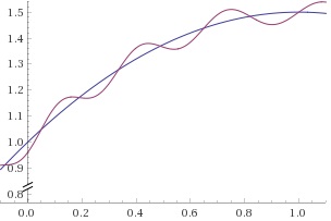
Figure 3.2. The function $f_{o}$ in (3.19) and (3.20) (a qualitative, rather than quantitative, picture).

In this setting, it holds that $f_{o}^{\prime}(r)=a_{2}-a_{3}\,r+\mu\phi^{\prime}(r)$ and therefore

$$\begin{split}&f_{o}^{\prime}\left(1+\bar{\vartheta}^{\frac{1}{2-s}}\right)=a_{2}-a_{3}-a_{3}\bar{\vartheta}^{\frac{1}{2-s}}+O(\mu)\\ {\mbox{and }}\;\;&f^{\prime\prime}_{o}\left(\bar{\vartheta}^{\frac{1}{2-s}}+\bar{\tau}^{\frac{1}{2-s}}\right)=-a_{3}+O(\mu).\end{split}$$ (3.21)

Furthermore,

$$\int_{0}^{1}\bar{\vartheta}^{\frac{1}{2-s}}\,d\bar{\vartheta}=\frac{2-s}{3-s}.$$ (3.22)

Hence, we insert (3.21) into (3.18), we exploit (3.22) and we obtain that

$$\begin{split}T^{s}\,{\mathcal{L}}u(L,T)\,=\,&-(2-s)\,\int_{0}^{1}\left(a_{2}-a_{3}-a_{3}\,\bar{\vartheta}^{\frac{1}{2-s}}\right)\,d\bar{\vartheta}-\int_{0}^{1}a_{3}\,d\bar{\tau}+\kappa\int_{0}^{1}a_{3}\,d\bar{\vartheta}+O(\mu)\\ =\,&-(2-s)(a_{2}-a_{3})+(2-s)\,a_{3}\cdot\frac{2-s}{3-s}-a_{3}+\kappa a_{3}+O(\mu)\\ =\,&a_{3}\,\left(\kappa-(2-s)\left(\frac{a_{2}}{a_{3}}-1\right)+\frac{(2-s)^{2}}{3-s}-1\right)+O(\mu).\end{split}$$ (3.23)

Therefore, the choice

$$\kappa:=(2-s)\left(\frac{a_{2}}{a_{3}}-1\right)-\frac{(2-s)^{2}}{3-s}+1$$ (3.24)

makes the leading order in the right hand side of (3.23) vanish. Notice also that $\kappa>0$ in the setting of (3.20). This yields that

$${\mathcal{L}}u(L,T)=O\left(\frac{\mu}{T^{s}}\right)=O(\delta\mu),$$ (3.25)

which is supposed to be a negligible quantity, for small $\delta$ and/or small $\mu$. In this approximation, we thus write (3.25) approximately as ${\mathcal{L}}u=0$, thus producing the fractional diffusion equation in (1.1), as desired.

It only remains to check the claim in (3.8), which is the goal of the forthcoming section.

Remark 3.1.

We observe that an alternative approach to (1.1) consists in introducing the dimensionless variables $\tilde{t}:=t/T$ and $\tilde{x}:=x/L$. Then, setting $\tilde{u}(\tilde{x},\tilde{t}):=u(L\tilde{x},T\tilde{t})$, equation (1.1) reduces to

$$D^{s}_{\tilde{t}}\tilde{u}=\kappa\partial^{2}_{\tilde{x}}\tilde{u}.$$

Notice that the coefficient $\kappa$ is expressed in terms of constants related to some properties of the travelling profiles (e.g., according to (3.24) for a small perturbation of a concave parabola).

We also recall again that such condition, as well as the derivation of (1.1), is obtained in (3.25) at the appropriate space/time scale $x:=L$ and $t:=T$, corresponding in the adimensional variables to the choice $\tilde{x}=\tilde{t}:=1$. More generally, one can think that the derived equation is valid on a small spatial scale around $L$ and a small temporal scale around $T$ (e.g. with $T$ and $L$ large, to make $\delta$ small in (3.12)).

4. Proof of (3.8)

By comparing the sum with the integrals, we see that, for each $k\in\{1,\dots,N\}$,

$$\int_{0}^{k}\frac{dx}{(x+1)^{\alpha}}\leqslant\sum_{1\leqslant j\leqslant{k}}\frac{1}{j^{\alpha}}\leqslant 1+\int_{1}^{k}\frac{dx}{x^{\alpha}}$$

and therefore

$$\frac{(k+1)^{1-\alpha}-1}{1-\alpha}\leqslant\sum_{1\leqslant j\leqslant{k}}\frac{1}{j^{\alpha}}\leqslant\frac{k^{1-\alpha}-\alpha}{1-\alpha}.$$ (4.1)

In particular, from (3.1) we have that

$$\frac{(N+1)^{1-\alpha}-1}{1-\alpha}\leqslant b_{N}\leqslant\frac{N^{1-\alpha}-\alpha}{1-\alpha}.$$

Accordingly, by (3.3),

$$\frac{\lambda_{k-1}}{L}=\frac{1}{b_{N}}\sum_{1\leqslant j\leqslant{k-1}}\frac{1}{j^{\alpha}}\in\left[\frac{k^{1-\alpha}-1}{N^{1-\alpha}-\alpha}\,,\;\frac{({k-1})^{1-\alpha}-\alpha}{(N+1)^{1-\alpha}-1}\right].$$ (4.2)

As a consequence,

$$\begin{split}&\left(\frac{k}{N}\right)^{1-\alpha}-\frac{\lambda_{k-1}}{L}\leqslant\left(\frac{{k}}{N}\right)^{1-\alpha}-\frac{k^{1-\alpha}-1}{N^{1-\alpha}-\alpha}\\ &\qquad=\left(\frac{{k}}{N}\right)^{1-\alpha}\,\left[1-\frac{1-\frac{1}{{k}^{1-\alpha}}}{1-\frac{\alpha}{N^{1-\alpha}}}\right].\end{split}$$ (4.3)

Now, for large $N$, we distinguish two cases, either ${k}\in[1,\sqrt{N}]$ or ${k}\in(\sqrt{N},N]$. If ${k}\in[1,\sqrt{N}]$, we deduce from (4.3) that

$$\left(\frac{{k}}{N}\right)^{1-\alpha}-\frac{\lambda_{k-1}}{L}\leqslant\left(\frac{{k}}{N}\right)^{1-\alpha}\leqslant\left(\frac{\sqrt{N}}{N}\right)^{1-\alpha}=\frac{1}{N^{\frac{1-\alpha}{2}}}.$$ (4.4)

If instead ${k}\in(\sqrt{N},N]$, we deduce from (4.3) that

$$\left(\frac{{k}}{N}\right)^{1-\alpha}-\frac{\lambda_{k-1}}{L}\leqslant 1-\frac{1-\frac{1}{k^{1-\alpha}}}{1-\frac{\alpha}{N^{1-\alpha}}}\leqslant 1-\frac{1-\frac{1}{{N}^{\frac{1-\alpha}{2}}}}{1-\frac{\alpha}{N^{1-\alpha}}}.$$ (4.5)

In any case, from (4.4) and (4.5), we have that

$$\left(\frac{{k}}{N}\right)^{1-\alpha}-\frac{\lambda_{k-1}}{L}\leqslant\frac{1}{N^{\frac{1-\alpha}{2}}}+\left|1-\frac{1-\frac{1}{{N^{\frac{1-\alpha}{2}}}}}{1-\frac{\alpha}{N^{1-\alpha}}}\right|.$$ (4.6)

In addition, from (4.2) we also have that

$$\begin{split}&\frac{\lambda_{k-1}}{L}-\left(\frac{{k}}{N}\right)^{1-\alpha}\leqslant\frac{({k-1})^{1-\alpha}-\alpha}{(N+1)^{1-\alpha}-1}-\left(\frac{{k}}{N}\right)^{1-\alpha}\\ &\qquad\leqslant\left(\frac{{k}}{N}\right)^{1-\alpha}\left[\frac{\left(\frac{k-1}{k}\right)^{1-\alpha}-\frac{\alpha}{k^{1-\alpha}}}{\left(\frac{N+1}{N}\right)^{1-\alpha}-\frac{1}{N^{1-\alpha}}}-1\right].\end{split}$$ (4.7)

Now, if $k\in[1,\sqrt{N}]$, we infer from (4.7) that

$$\begin{split}&\frac{\lambda_{k-1}}{L}-\left(\frac{{k}}{N}\right)^{1-\alpha}\leqslant 2\,\left(\frac{{k}}{N}\right)^{1-\alpha}\leqslant 2\,\left(\frac{\sqrt{N}}{N}\right)^{1-\alpha}=\frac{2}{N^{\frac{1-\alpha}{2}}}.\end{split}$$ (4.8)

If instead ${k}\in(\sqrt{N},N]$, we deduce from (4.7) that

$$\frac{\lambda_{k-1}}{L}-\left(\frac{{k}}{N}\right)^{1-\alpha}\leqslant\frac{\left(\frac{k-1}{k}\right)^{1-\alpha}-\frac{\alpha}{k^{1-\alpha}}}{\left(\frac{N+1}{N}\right)^{1-\alpha}-\frac{1}{N^{1-\alpha}}}-1\leqslant\frac{1-\frac{\alpha}{N^{1-\alpha}}}{1-\frac{1}{N^{1-\alpha}}}-1.$$

In any case, recalling (4.8), we have that for every $k\in\{1,\dots,N\}$ it holds that

$$\frac{\lambda_{k-1}}{L}-\left(\frac{{k}}{N}\right)^{1-\alpha}\leqslant\frac{2}{N^{\frac{1-\alpha}{2}}}+\left|\frac{1-\frac{\alpha}{N^{1-\alpha}}}{1-\frac{1}{N^{1-\alpha}}}-1\right|.$$

Hence, in view of (3.7) and (4.6), we have that

$$\frac{|\eta_{k,N}|}{L}={\left|\left(\frac{k}{N}\right)^{1-\alpha}-\frac{\lambda_{k-1}}{L}\right|}\leqslant\frac{3}{N^{\frac{1-\alpha}{2}}}+\left|1-\frac{1-\frac{1}{{N^{\frac{1-\alpha}{2}}}}}{1-\frac{\alpha}{N^{1-\alpha}}}\right|+\left|\frac{1-\frac{\alpha}{N^{1-\alpha}}}{1-\frac{1}{N^{1-\alpha}}}-1\right|,$$

and this plainly implies (3.8), as desired.

5. Conclusions

Purkinje cells seem to exhibit two special features:

1. on the one hand, their malfunction is related, among the others, to abrupt movements, tremors and lack of coordination;

2. on the other hand, recent experiments have shown the evidence of time fractional diffusion arising in Purkinje cells.

Also, in the mathematical theory of evolution equations, typically two regularity regimes arise:

1. on the one hand, hyperbolic equations typically present shocks and irregular solutions;

2. on the other hand, parabolic equations are endowed with good regularity theories with respect to the initial data.

It is quite tempting to relate the biological phenomena in (i)–(ii) with the mathematical treats in (i)’-(ii)’, respectively. In this paper, we provide a mathematical setting to show how highly ramified media affect the propagation of travelling waves, by producing a superposition of delayed signals which in turn may be related to time fractional diffusion.

In our computation, we derive the time fractional heat equation as the effect of the superposition of delayed classical heat equations, measured at a spatial scale in proximity of the end of the transmission network and at a time close to the characteristic diffusion time. The delay in the fundamental heat equation is produced by a network, in which the length of each branch is appropriately chosen to produce a suitable superposition effect.

Our expansion is calculated on a specific travelling wave, taken as a small perturbation of a concave parabola, and the diffusion coefficient depends on the slope and on the curvature of such travelling profile.

The remainders of our formula are explicitly stated and the asymptotics are discussed in details. To emphasize the role of the scales at which the main equation is attained (up to remainders), one can also rewrite the dimensional time fractional heat equation in terms of adimensional space and time variables.

In our mathematical framework, we show that highly ramified media may provide a regularizing effect on the leading equations of signal transmission. It is of course intriguing to relate the ramification of these underlying mathematical media with the structure of the Purkinje neuron’s dendritic arbor.

We also recall that usually fractional diffusion is discussed mostly in relation to its classical parabolic analogue (for instance, it is commonly viewed that “the appearance of fractional equations is very appealing due to their proximity to the analogous standard equations”, see page 5 in [37]). In this sense, from the theoretical point of view, our approach seems to be rather different from the existing literature and the new link that we propose between fractional diffusion and hyperbolic (rather than parabolic) equations may lead to stimulating mathematical considerations from a different perspective.

References

- [1] N. Abatangelo, E. Valdinoci: Getting acquainted with the fractional Laplacian. To appear in Springer INdAM Ser.
- [2] M. Allen: A Nondivergence Parabolic Problem with a Fractional Time derivative. Differential Integral Equations 31, no. 3-4 (2018), 215–230.
- [3] M. Allen, L. Caffarelli, A. Vasseur: A parabolic problem with a fractional time derivative. Arch. Ration. Mech. Anal. 221, no. 2 (2016), 603–630.
- [4] T. J. Anastasio: Nonuniformity in the linear network model of the oculomotor integrator produces approximately fractional-order dynamics and more realistic neuron behavior. Biol Cybern. 79 (1998), 377–391.
- [5] R. Appali, U. van Rienen, T. Heimburg: A comparison of the Hodgkin-Huxley model the soliton theory for the action potential in nerves. Adv. Planar Lipid Bilayers Liposomes 16 (2012), 275–298.
- [6] R. Bagley: On the equivalence of the Riemann-Liouville and the Caputo fractional order derivatives in modeling of linear viscoelastic materials. Fract. Calc. Appl. Anal. 10 (2007), no. 2, 123–126.
- [7] C. A. Balanis: Advanced engineering electromagnetics. John Wiley & Sons, 2012.
- [8] D. ben-Avraham, S. Havlin: Diffusion and reactions in fractals and disordered systems. Cambridge University Press, Cambridge, 2000.
- [9] A. Blanco, R. Moyano, J. Vivo, R. Flores-Acuña, A. Molina, C. Blanco, J. G. Monterde: Purkinje cell apoptosis in arabian horses with cerebellar abiotrophy. J. Vet. Med. Physiol. Pathol. Clin. Med. 53, no. 6 (2006), 286–287.
- [10] C. Bucur: Local density of Caputo-stationary functions in the space of smooth functions. ESAIM Control Optim. Calc. Var. 23, no. 4 (2017), 1361–1380.
- [11] C. Bucur, E. Valdinoci: Nonlocal diffusion and applications. Lecture Notes of the Unione Matematica Italiana 20. Springer, Bologna, 2016.
- [12] M. Caputo: Linear model of dissipation whose is almost frequency independent-II. Geophys. J. R. Astron. Soc. 13, no. 5 (1967), 529–539.
- [13] S. Coombes: Neural fields. Scholarpedia 1, no. 6 (2006), 1373.
- [14] R. Dáger, E. Zuazua: Wave propagation, observation and control in -d flexible multi-structures. Mathématiques & Applications, 50. Springer-Verlag, Berlin, 2006.
- [15] K. Diethelm: The analysis of fractional differential equations. An application-oriented exposition using differential operators of Caputo type. Lecture Notes in Mathematics. Springer, Berlin, 2004.
- [16] S. Dipierro, O. Savin, E. Valdinoci: All functions are locally -harmonic up to a small error. J. Eur. Math. Soc. (JEMS) 19 (2017), no. 4, 957–966.
- [17] S. Dipierro, O. Savin, E. Valdinoci: Local approximation of arbitrary functions by solutions of nonlocal equations. ArXiv 1609.04438 (2016).
- [18] M. Du, Z. Wang, H. Hu. Measuring memory with the order of fractional derivative. Sci. Rep. 3 (2013), 3431.
- [19] A. El Hady, B. B. Machta: Mechanical surface waves accompany action potential propagation. Nature Comm. 6 (2015), 6697 EP.
- [20] G. B. Ermentrout, D. Kleinfeld: Traveling electrical waves in cortex: Insights from phase dynamics and speculation on a computational role. Neuron 29 (2001), 33–44.
- [21] G. B. Ermentrout, J. B. McLeod: Existence and uniqueness of travelling waves for a neural network. Proc. Royal Soc. Edinburgh 123A (1993), 461–478.
- [22] L. C. Evans: Partial differential equations. Graduate Studies in Mathematics, 19. American Mathematical Society, Providence, RI, 1998.
- [23] J. C. Fiala, K. M. Harris: Dendrite structure. In G. Stuart, S. Nelson, and M. Häusser, eds.: Dendrites. Oxford Scholarship Online. Oxford University Press, Oxford, 1999.
- [24] A. Gonzalez-Perez, L. D. Mosgaard, R. Budvytyte, E. Villagran-Vargas, A. D. Jackson, T. Heimburg: Solitary electromechanical pulses in lobster neurons, Bioph. Chem. 216 (2016), 51–59.
- [25] T. Heimburg, A. D. Jackson: On soliton propagation in biomembranes and nerves. Proc. Nat. Acad. Sci. 102, no. 28 (2005), 9790–9795.
- [26] A. L. Hodgkin, A. F. Huxley: A quantitative description of membrane current and its application to conduction and excitation in nerve. J. Physiology 117, no. 4 (1952), 500–544.
- [27] C. Ionescu, A. Lopes, D. Copot, J. A. T. Machado, J. H. T. Bates: The role of fractional calculus in modelling biological phenomena: a review. Comm. Nonlin. Science Numer. Simul. 51 (2017), 141–159.
- [28] V. G. Ivancevic, T. T. Ivancevic: Quantum Neural Computation. Springer, Netherlands, 2010.
- [29] J. J. Karakash: Transmission Lines and Filter Networks. Macmillan, New York, 1950.
- [30] I. Kim, K.-H. Kim, S. Lim: An -theory for the time fractional evolution equations with variable coefficients. Adv. Math. 306 (2017), 123–176.
- [31] M. E. Larkum, S. Watanabe, T. Nakamura, N. Lasser-Ross, W. N. Ross: Synaptically activated Ca2+ waves in layer 2/3 and layer 5 rat neocortical pyramidal neurons. J. Physiol. 549 (2003), 471–488.
- [32] B. Lautrup, R. Appali, A. D. Jackson, T. Heimburg: The stability of solitons in biomembranes and nerves. Eur. Phys. J. 34, no. 57 (2011), 1–9.
- [33] R. L. Magin: Fractional calculus models of complex dynamics in biological tissues. Computers Math. Appl. 59 (2010), 1586–1593.
- [34] T. Marinov, F. Santamaria: Modeling the effects of anomalous diffusion on synaptic plasticity. BMC Neuroscience 14, Suppl. 1 (2013), P343.
- [35] T. Marinov, F. Santamaria: Computational modeling of diffusion in the cerebellum. Prog. Mol. Biol. Transl. Sci. 123 (2014), 169–89.
- [36] I. A. Mavroudis, D. F. Fotiou, L. F. Adipepe, M. G. Manani, S. D. Njau, D. Psaroulis, V. G. Costa, S. J. Baloyannis: Morphological changes of the human purkinje cells and deposition of neuritic plaques and neurofibrillary tangles on the cerebellar cortex of Alzheimer’s disease. Amer. J. Alzheimer’s Dise. Other Dem. 25, no. 7 (2010), 585–591.
- [37] R. Metzler, J. Klafter: The random walk’s guide to anomalous diffusion: A fractional dynamics approach. Phys. Rep. 339, no. 1 (2000), 1–77.
- [38] W. L. Miranker: A neural network wave formalism. Adv. Appl. Math., 37 (2006) 19–30.
- [39] T. Nakamura, N. Lasser-Ross, K. Nakamura, W. N. Ross: Spatial segregation and interaction of calcium signalling mechanisms in rat hippocampal CA1 pyramidal neurons. J. Physiol. 543 (2002), 465–480.
- [40] S. A. Neymotin, R. A. McDougal, M. A. Sherif, C. P. Fall, M. L. Hines, W. W. Lytton: Neuronal Calcium wave propagation varies with changes in endoplasmic reticulum parameters: a computer model. Neural Comp. 27, no. 4 (2015), 898–924.
- [41] E. A. Nimchinsky, B. L. Sabatini, K. Svoboda: Structure and function of dendritic spines. Annu. Rev. Physiol. 64 (2002), 313–353.
- [42] D. J. Pinto, G. B. Ermentrout: Spatially structured activity in synaptically coupled neuronal networks: I. Travelling fronts and pulses. SIAM J. Applied Math., 62 (2001), 206–225.
- [43] G. G. Rigatos: Advanced Models of Neural Networks. Nonlinear Dynamics and Stochasticity in Biological Neurons. Springer-Verlag, Berlin, 2015.
- [44] W. N. Ross: Understanding calcium waves and sparks in central neurons. Nature Rev. Neurosci. 13 (2002), 157–168.
- [45] E. È. Saftenku: Modeling of slow glutamate diffusion and AMPA receptor activation in the cerebellar glomerulus. J. Theor. Biology 234 (2005), 363–382.
- [46] F. Santamaria, S. Wils, E. De Schutter, G. J. Augustine: Anomalous Diffusion in Purkinje Cell Dendrites Caused by Spines. Neuron 52 (2006), 635–648.
- [47] F. Santamaria, S. Wils, E. De Schutter, G. J. Augustine: The diffusional properties of dendrites depend on the density of dendritic spines. Europ. J. Neuroscience 34, no. 4 (2011), 561–568.
- [48] M. J. Saxton: Anomalous diffusion due to binding: a Monte Carlo study. Biophys. J. 70 (1996), 1250–1262.
- [49] E. R. von Schweidler: Studien über die Anomalien im Verhalten der Dielectrika. Ann. Phys. 24, (1907), 711–770.
- [50] J. Thorson, M. Biederman-Thorson: Distributed relaxation processes in sensory adaptation: spatial nonuniformity in receptors can explain both the curious dynamics and logarithmic statics of adaptation. Science 183, no. 4121 (1974), 161–172.
- [51] J. Trommershäuser, J. Marienhagen, A. Zippelius: Stochastic Model of Central Synapses: Slow Diffusion of Transmitter Interacting with Spatially Distributed Receptors and Transporters. J. Theor. Biology 198 (1999), 101–120.
-
[52]
Wikipedia:
Drawing of Purkinje cells (A) and granule cells (B)
from pigeon cerebellum by Santiago Ramón y Cajal, 1899;
Instituto Cajal, Madrid, Spain.
File:PurkinjeCell.jpg
https://en.wikipedia.org/wiki/Purkinje_cell#/media/File:PurkinjeCell.jpg - [53] R. Zacher: Maximal regularity of type for abstract parabolic Volterra equations. J. Evol. Equ. 5, no. 1 (2005), 79–103.
- [54] R. Zacher: A De Giorgi-Nash type theorem for time fractional diffusion equations. Math. Ann. 356, no. 1 (2013), 99–146.