Non-toric Cones and Chern-Simons Quivers

ABSTRACT

We obtain an integral formula for the volume of non-toric tri-Sasaki Einstein manifolds arising from nonabelian hyperkähler quotients. The derivation is based on equivariant localization and generalizes existing formulas for Abelian quotients, which lead to toric manifolds. The formula is particularly valuable in the context of AdS${}_{4}\times Y_{7}$ vacua of M-theory and their field theory duals. As an application, we consider 3d ${\cal N}=3$ Chern-Simons theories with affine ADE quivers. While the $\widehat{A}$ series corresponds to toric $Y_{7}$, the $\widehat{D}$ and $\widehat{E}$ series are non-toric. We compute the volumes of the corresponding seven-manifolds and compare to the prediction from supersymmetric localization in field theory, finding perfect agreement. This is the first test of an infinite number of non-toric AdS₄/CFT₃ dualities.

1 Introduction

Sasaki-Einstein manifolds play an important role in AdS/CFT. These odd-dimensional manifolds, with the property that the cones over them are Calabi-Yau, appear naturally in the engineering of supersymmetric gauge theories by branes in string/M-theory. Their first appearance in holography was in the context of AdS₅/CFT₄. Placing $N$ D3-branes at the tip of a Calabi-Yau cone $\mathcal{C}(Y_{5})$, and backreacting the branes, leads to an AdS${}_{5}\times Y_{5}$ vacuum of Type IIB supergravity with a 4d ${\cal N}=1$ field theory dual. Following the first example of the conifold singularity ${\cal C}(T^{1,1})$ [1], a vast number of new dualities were discovered by the explicit construction of an infinite family of Sasaki-Einstein metrics [2], and the subsequent identification of their field theory duals as quiver gauge theories [3, 4].

Similar developments have followed in the case of AdS₄/CFT₃. Placing $N$ M2-branes at the tip of a hyperkähler cone $\mathcal{C}(Y_{7})$, where $Y_{7}$ is a tri-Sasaki-Einstein manifold now, and backreacting the branes leads to an AdS${}_{4}\times Y_{7}$ vacuum of M-theory with a 3d ${\cal N}=3$ field theory dual. Following the first explicit example by ABJM [5], a large number of dual pairs have been identified, with $Y_{7}$ given by the base of certain hyperkähler cones and the field theories corresponding to 3d ${\cal N}=3$ Chern-Simons (CS) quiver gauge theories [6, 7, 8, 9, 10, 11].

Computing the volume of these manifolds is of great interest as the AdS/CFT dictionary relates $\operatorname{Vol}(Y)$ to important nonperturbative quantities in field theory. For instance, in the case of D3-branes the $a$–anomaly coefficient of the 4d field theory is given by $a=\frac{\pi^{3}N^{2}}{4\operatorname{Vol}(Y_{5})}$. In the case of M2-branes the free energy on the round three-sphere $F_{S^{3}}$ is given by [12, 7]

$$F_{S^{3}}=N^{3/2}\sqrt{\frac{2\pi^{6}}{27\operatorname{Vol}(Y_{7})}}\,.$$ (1.1)

The independent evaluation of both sides of this relation has been crucial in providing convincing evidence for the proposed duality pairs. The LHS can be computed purely in field theory by supersymmetric localization [13] and has been carried out for a large number of CS quiver gauge theories [13, 7, 12, 8, 9, 10, 11, 14, 15, 16]. The RHS, however, has been mostly computed for toric $Y_{7}$, and a detailed test of the duality for non-toric cases is lacking. The main reason for this is that although supersymmetric localization techniques are available on the field theory side for generic quivers, less tools are available on the geometry side for non-toric $Y_{7}$.

The aim of this paper is to remedy this situation. Specifically, we provide a formula for computing the volumes of tri-Sasaki Einstein manifolds $Y_{4d-1}$ arising from nonabelian hyperkähler quotients of the form ${\cal C}(Y_{4d-1})=\mathbb{H}^{d+∑_{a=1}^{m}n_{a}^{2}}///U(n_{1})\times\cdots\times U(n_{m})\,$. The derivation is based on the method of equivariant localization, making use of the $U(1)_{R}\subset SU(2)_{R}$ symmetry of the spaces. The localization method was developed in [19, 20] and applied to toric hyperkähler quotients, corresponding to the Abelian case, $n_{a}=1$, by Yee in [21].

Having derived a general formula, our main application is to 3d ${\cal N}=3$ CS matter quiver theories, whose field content is in one-to-one correspondence with extended ADE Dynkin diagrams – see Figure 1.

Figure 1: Affine ADE quivers. From top to bottom and left to right $\widehat{A}_{n},\widehat{D}_{n},\widehat{E}_{6},\widehat{E}_{7},\widehat{E}_{8}$

These theories [22] provide an ideal setting for applying the volume formula derived using localization. First, the corresponding tri-Sasaki Einstein manifolds can be constructed by hyperkähler quotients and, while the $\widehat{A}$ series is toric, the $\widehat{D}$ and $\widehat{E}$ series are non-toric. Second, as shown in [22] for this class of field theories one may apply the saddle point approximation developed in [7] to evaluate the free energy at large $N$. For the $\widehat{A}$ series, both the evaluation of the free energy as well as the direct computation of the corresponding toric volume was carried out in [8], with perfect agreement. For the $\widehat{D}$ and $\widehat{E}$ series, the free energy was computed by the authors in [16]. In this paper we focus on the geometric side of the $\widehat{D}$ series, identifying the precise tri-Sasaki Einstein manifolds and computing their volumes, finding perfect agreement with field theory. This is the first test of an infinite number of non-toric AdS₄/CFT₃ dualities. Few non-toric examples have been studied in the AdS₅/CFT₄ context; it is our hope that the formulas presented here will also be valuable in that context.

The paper is organized as follows. In the next section, we set up the localization procedure for computing the volumes of hyperkähler quotients involving $U(N)$ or $SU(N)$ groups. Then, in section 3 we specialize to $SU(2)^{s}×U(1)^{r}$ and provide a simple example. Finally, in section 4 we study the moduli space of 3d ${\cal N}=3$ CS $\widehat{D}$–quiver theories, identify the dual tri-Sasaki Einstein manifolds and compute their volumes. The volumes in the case of $\widehat{E}$–quivers can also be computed by the techniques presented here, but we do not explicitly perform the corresponding integrals.

2 Localization Setup

In this section, we give a brief overview of the technical tools necessary for the computation of the volumes of hyperkähler cones. The method was developed in [19, 20] and is based on two basic features of the object we wish to compute. The first feature is the existence of a fermionic nilpotent symmetry of the symplectic volume integral, which allows one to localize the integral by adding an appropriate exact term. The second feature is that since these manifolds arise from hyperkähler quotients of flat space, one may formulate the calculation in terms of the embedding flat space, where the calculations become simpler. We follow the exposition of Yee [21] (which we urge the reader to refer for more details), where this approach was applied to toric hyperkähler quotients, and extend it to non-toric quotients.

Given a bosonic manifold $X$, and its tangent bundle $TX$ with canonical coordinates $\{x^{\mu},V^{\mu}\}$, one defines the supermanifold $T[\psi]X$ obtained by replacing the bosonic coordinates $\{V^{\mu}\}$ with fermionic ones $\{\psi^{\mu}\}$. Integrals of differential forms on $X$ can then be written as integrals of functions $f(x,\psi)$ over $T[\psi]X$. For instance, the volume of a symplectic manifold $X$ with symplectic 2-form $ω=\tfrac{1}{2}ω_{μν}ψ^{μ}ψ^{ν}$ can be written as

$$\operatorname{Vol}(X)=∫_{T[ψ]X}e^{ω}\,;$$ (2.1)

the Grassmann integration simply picks the correct power of $\omega$ to give the volume form on $X$. One may view this expression as a supersymmetric partition function; defining a ‘supersymmetry charge’ $Q=ψ^{μ}\frac{∂}{∂x^{μ}}$ (which is the de Rham differential, $d$), we see that the ‘action’ $S=ω$ is supersymmetric, as $Qω=0$ (usually written as $dω=0$). Na\̈dot{\iota}vely, one may want to use this nilpotent fermionic symmetry, $Q^{2}=0$, to localize the integral. However, because $Q$ always contains a $\psi^{\mu}$, there is no $Q$–exact term one can add to the action which contains a purely bosonic term, required by the usual localization arguments. One way around this is to use a global symmetry of $\omega$ to deform $Q\textrightarrow{Q}_{\varepsilon}$. Given a symmetry–generating vector field $V=V^{μ}\frac{∂}{∂x^{μ}}$ and defining the ‘contraction’ by $V$ as $i_{V}=V^{μ}\frac{∂}{∂ψ^{μ}}$, there is a function $H$ such that $QH=i_{V}ω$, which can be named Hamiltonian, moment map, etc. depending on the context. This function $H$ can be used to deform the action to $S_{\varepsilon}=ω-\varepsilon H$, which is now invariant under ${Q}_{\varepsilon}=ψ^{μ}\frac{∂}{∂x^{μ}}+\varepsilon V^{μ}(x)\frac{∂}{∂ψ^{μ}}$. Moreover, ${Q}_{\varepsilon}^{2}=\varepsilon{\cal L}_{V}$ with the Lie derivative ${\cal L}_{V}=\{i_{V},Q\}$, which implies that ${Q}_{\varepsilon}$ is nilpotent in the subspace of $V$–invariant functions on $T[ψ]X$. This deformation now allows the addition of bosonic terms (with an $\varepsilon$–dependence) and localization can be performed. The next step is to combine this with the fact that the Kähler spaces of interest are obtained from a Kähler quotient of flat space.

Kähler Quotient.

Given a Kähler manifold $M$ with Kähler form $\omega$ and a holomorphic symmetry $G$, generated by vector fields $V_{v}$, $v=1,⋯,\dim G$, it follows from $\mathcal{L}_{V_{v}}\omega=0$ that there are a set of moment map functions $μ_{v}$ satisfying $i_{V_{v}}ω=Qμ_{v}$. The Lie derivative ${\cal L}_{V_{v}}$ acts on the moment maps as follows

$$V_{v}^{μ}\frac{∂μ_{u}(x)}{∂x^{μ}}=i_{V_{v}}(Qμ_{u})=i_{V_{v}}i_{V_{u}}ω=f_{uv}{}^{w}μ_{w}(x)\,,$$ (2.2)

where $f_{uv}{}^{w}$ are the structure constants of $G$. The submanifold $μ_{v}^{-1}(0)$ is $V$–invariant and the Kähler quotient $M//G$ is defined as the usual quotient $μ_{v}^{-1}(0)/G$. Parameterizing $M$ by splitting $\{x^{μ}\}$ into three parts $\{x^{i},x^{v},x^{n}\}$, such that $x^{i}\in μ^{-1}(0)/G$, $x^{v}$ denote the symmetry directions, i.e., $V_{u}=V_{u}^{v}\frac{∂}{∂x^{v}}$, and $x^{n},n=1,⋯,\dim G$ are coordinates normal to $μ_{v}^{-1}(0)$, we can derive the following relations from $Qμ_{v}=i_{V_{v}}ω$:

$$∂_{i}μ_{v}=ω_{vi}\,,\qquad∂_{u}μ_{v}=ω_{vu}\,,\qquad∂_{n}μ_{v}=ω_{vn}\,.$$ (2.3)

Since $μ_{v}=0$ on $μ_{v}^{-1}(0)$, its derivative wrt $x^{i}$, $ω_{vi}=0$ on $μ_{v}^{-1}(0)$. Also, $ω_{vu}=0$ as $V_{v}^{μ}\frac{∂μ_{u}(x)}{∂x^{μ}}=0$ on $μ_{v}^{-1}(0)$. Thus, $Qω=0$ gives $∂_{v}ω_{ij}=∂_{i}ω_{vj}-∂_{j}ω_{vi}=0$ so $ω_{ij}$ is $V$–invariant on $μ_{v}^{-1}(0)$ and the Kähler quotient then inherits $ω_{ij}$ as its Kähler form. Using (2.1), the volume of the quotient manifold can be written as

$$\operatorname{Vol}\left(M//G\right) =∫_{T[ψ]μ_{v}^{-1}(0)/G}[dx^{i}][dψ^{i}]\,e^{\frac{1}{2}ω_{ij}ψ^{i}ψ^{j}}$$

$$=\frac{1}{\operatorname{Vol}\left(G\right)}∫_{T[ψ]μ_{v}^{-1}(0)}[dx^{v}][dx^{i}][dψ^{i}]\,e^{\frac{1}{2}ω_{ij}ψ^{i}ψ^{j}}$$

$$=\frac{1}{\operatorname{Vol}\left(G\right)}∫_{T[ψ]M}[dx^{n}][dx^{v}][dx^{i}][dψ^{i}]\,e^{\frac{1}{2}ω_{ij}ψ^{i}ψ^{j}}∏_{v=1}^{\dim G}δ\left(μ_{v}(x)\right)\left|\frac{∂μ_{v}(x)}{∂x^{n}}\right|$$

$$=\frac{1}{(2π)^{\dim G}\operatorname{Vol}\left(G\right)}∫_{T[ψ]M}[dφ^{v}][dψ^{v}][dψ^{n}][dx^{μ}][dψ^{i}]\,e^{\frac{1}{2}ω_{ij}ψ^{i}ψ^{j}}e^{\dot{\iota}φ^{v}μ_{v}+ψ^{v}ω_{vn}ψ^{n}}.$$

What these steps have achieved is to insert and exponentiate the moment map constraints to turn an integral over the quotient space $M//G$ into an integral over the embedding space $M$. Now, we use $ω_{vi}=ω_{vu}=0$ to write $ψ^{v}ω_{vn}ψ^{n}=ψ^{v}ω_{vμ}ψ^{μ}$, where $μ$ runs over all values in $M$ (like $x^{μ}$). Next, inserting $ω_{in}$ and $ω_{mn}$ terms, which can be absorbed by shifting $ψ^{i}\textrightarrow ψ^{i}-ω_{ji}^{-1}ω_{jn}ψ^{n}$ and $ψ^{v}\textrightarrow ψ^{v}-ω_{nv}^{-1}ω_{nm}ψ^{m}$, to complete the $ω_{μν}ψ^{μ}ψ^{ν}$ term, leads to the following simple expression:

$$\operatorname{Vol}\left(M//G\right)=\frac{1}{(2π)^{\dim G}\operatorname{Vol}\left(G\right)}∫_{T[ψ]M⊗φ^{v}}e^{ω+\dot{\iota}φ^{v}μ_{v}}.$$ (2.4)

One may further make use of the $U(1)_{R}$ symmetry to introduce the $\varepsilon$–deformation

$$\operatorname{Vol}_{\varepsilon}\left(M//G\right)=\frac{1}{(2π)^{\dim G}\operatorname{Vol}\left(G\right)}∫_{T[ψ]M⊗φ^{v}}e^{ω+\dot{\iota}φ^{v}μ_{v}-\varepsilon H}\,$$ (2.5)

and compute this integral by localization. When $M$ is multiple copies of the complex plane $\mathbb{C}$ with its canonical structures, the $\psi$–integrals are trivial and simply give 1. With appropriate $H$, the $x$–integrals are Gaussian and only the integrals over $φ$’s remain, which require some more work to perform. The case of $M//G$ a conical Calabi-Yau six-fold is of interest for AdS₅/CFT₄. However, it should be emphasized that the expression above computes the volume wrt the quotient metric, which is not necessarily (and typically is not) the Calabi-Yau metric on $M//G$. For this reason, we focus in what follows on hyperkähler quotients, where the Calabi-Yau condition is automatic.

Hyperkähler Quotient.

A hyperkähler manifold $M$ with a triplet of Kähler forms $\vec{ω}$ and a tri-holomorphic isometry group $G$ has triplets of moment maps satisfying $i_{V_{v}}\vec{ω}=Q\vec{μ}_{v}$. Most of what follows is a straightforward generalization of the Kähler case so we write down the most important equations only. The Lie derivative ${\cal L}_{V_{v}}$ acts on the moment maps as follows

$$V_{v}^{μ}\frac{∂\vec{μ}_{u}(x)}{∂x^{μ}}=i_{V_{v}}(Q\vec{μ}_{u})=i_{V_{v}}i_{V_{u}}\vec{ω}=f_{uv}{}^{w}\vec{μ}_{w}(x)\,.$$ (2.6)

The submanifold $\vec{μ}_{v}^{-1}(0)$ is $V$–invariant so the hyperkähler quotient $M///G$ is defined [25] as the usual quotient $\vec{μ}_{v}^{-1}(0)/G$ . Parameterizing $M$ by $\{x^{i},x^{v},x^{n}\}$, where the only difference wrt the Kähler case is that $n=1,⋯,3\dim G$, we can derive from $Q\vec{μ}_{v}=i_{V_{v}}\vec{ω}$:

$$∂_{i}\vec{μ}_{v}=\vec{ω}_{vi}\,,\qquad∂_{u}\vec{μ}_{v}=\vec{ω}_{vu}\,,\qquad∂_{n}\vec{μ}_{v}=\vec{ω}_{vn}\,.$$ (2.7)

Again $\vec{ω}_{vi}=0$ and $\vec{ω}_{vu}=0$ on $\vec{μ}_{v}^{-1}(0)$. Thus, $Q\vec{ω}=0$ gives $∂_{v}\vec{ω}_{ij}=∂_{i}\vec{ω}_{vj}-∂_{j}\vec{ω}_{vi}=0$ so $\vec{ω}_{ij}$ is $V$–invariant on $\vec{μ}_{v}^{-1}(0)$ and the hyperkähler quotient then inherits $\vec{ω}_{ij}$ as its 3 Kähler forms. We pick $ω^{3}=ω$ to define the volume as

$$\operatorname{Vol}\left(M///G\right) =∫_{T[ψ]\vec{μ}_{v}^{-1}(0)/G}[dx^{i}][dψ^{i}]\,e^{\frac{1}{2}ω_{ij}ψ^{i}ψ^{j}}$$

$$=\frac{1}{\operatorname{Vol}\left(G\right)}∫_{T[ψ]\vec{μ}_{v}^{-1}(0)}[dx^{v}][dx^{i}][dψ^{i}]\,e^{\frac{1}{2}ω_{ij}ψ^{i}ψ^{j}}$$

$$=\frac{1}{\operatorname{Vol}\left(G\right)}∫_{T[ψ]M}[dx^{n}][dx^{v}][dx^{i}][dψ^{i}]\,e^{\frac{1}{2}ω_{ij}ψ^{i}ψ^{j}}∏_{v=1}^{\dim G}∏_{a=1}^{3}δ\left(μ^{a}_{v}(x)\right)\left|\frac{∂μ^{a}_{v}(x)}{∂x^{n}}\right|$$

$$=\frac{1}{(2π)^{3\dim G}\operatorname{Vol}\left(G\right)}∫_{T[ψ]M}[d\vec{φ}^{v}][d\vec{χ}^{v}][dψ^{n}][dx^{μ}][dψ^{i}]\,e^{\frac{1}{2}ω_{ij}ψ^{i}ψ^{j}}e^{\dot{\iota}\vec{φ}^{v}·\vec{μ}_{v}+\vec{χ}^{v}·\vec{ω}_{vn}ψ^{n}}.$$

Again, these steps have turned an integral over $M///G$ to an integral over $M$. Now, using $\vec{ω}_{vi}=\vec{ω}_{vu}=0$ and relabelling $χ^{v}_{3}=ψ^{v}$ we rewrite $χ^{v}_{3}ω_{vn}ψ^{n}=ψ^{v}ω_{vμ}ψ^{μ}$. Similarly, $χ^{v}_{a}ω^{a}_{vn}ψ^{n}=χ^{v}_{a}Qμ^{a}_{v}$, where $a=1,2$ now. Further relabelling $φ^{v}_{3}\textrightarrow φ^{v}$ and $φ^{v}_{a}\textrightarrow ρ^{v}_{a}$ and inserting $ω_{in}$ and $ω_{mn}$ pieces, which can be absorbed by shifting $ψ$’s as before, one completes the $ω_{μν}ψ^{μ}ψ^{ν}$ term to obtain a simplified exponent:

$$\operatorname{Vol}\left(M///G\right)=\frac{1}{(2π)^{3\dim G}\operatorname{Vol}\left(G\right)}∫_{T[ψ]M⊗φ^{v}⊗\{ρ^{v}_{a},χ^{v}_{a}\}}e^{ω+\dot{\iota}φ^{v}μ_{v}+\dot{\iota}ρ^{v}_{a}μ^{a}_{v}+χ^{v}_{a}Qμ^{a}_{v}}.$$ (2.8)

The ‘action’ $S=ω+\dot{\iota}φ^{v}μ_{v}+\dot{\iota}ρ^{v}_{a}μ^{a}_{v}+χ^{v}_{a}Qμ^{a}_{v}$ is invariant under a modified charge $\tilde{Q}$, acting on the ‘coordinates’ as follows:

$$\begin{aligned} \tilde{Q}x^{μ}&=ψ^{μ}\\ \tilde{Q}ψ^{μ}&=-\dot{\iota}φ^{v}V_{v}^{μ}(x)\\ \tilde{Q}φ^{v}&=0\\ \tilde{Q}χ^{u}_{a}&=-\dot{\iota}ρ^{u}_{a}\\ \tilde{Q}ρ^{u}_{a}&=-\dot{\iota}f_{vw}{}^{u}φ^{v}χ^{w}_{a}\,.\end{aligned}$$ (2.9)

The transformation $\tilde{Q}ρ^{u}_{a}$ is fundamentally different from the toric case (where it vanishes), as a consequence of the action of ${\cal L}_{V_{v}}$ on the moment maps (2.6). However, it still squares as $\tilde{Q}^{2}=-\dot{\iota}φ^{v}{\cal L}_{V_{v}}$. Now we make use of the $U(1)_{R}\subset SU(2)_{R}$ symmetry to introduce the $\varepsilon$–deformation and compute the integral by localization. This symmetry preserves only $ω^{3}=ω$, such that $i_{R}ω=QH$, and rotates the other two as ${\cal L}_{R}(ω^{1}-\dot{\iota}ω^{2})=2\dot{\iota}(ω^{1}-\dot{\iota}ω^{2})$ $\big{(}$also ${\cal L}_{R}(μ^{1}_{v}-\dot{\iota}μ^{2}_{v})=2\dot{\iota}(μ^{1}_{v}-\dot{\iota}μ^{2}_{v})$ for all $v\big{)}$. The deformed action $S_{\varepsilon}=S-\varepsilon H$ is invariant under the deformed supercharge $\tilde{Q}_{\varepsilon}$, which acts differently from $\tilde{Q}$ only on $ψ^{μ}$ and $ρ^{u}_{a}$, namely:

$$\begin{aligned} \tilde{Q}_{\varepsilon}ψ^{μ}&=-\dot{\iota}φ^{v}V_{v}^{μ}(x)+\varepsilon R^{μ}(x)\\ \tilde{Q}_{\varepsilon}ρ^{u}_{a}&=-\dot{\iota}f_{vw}{}^{u}φ^{v}χ^{w}_{a}+2\varepsilon ε_{ab}χ^{u}_{b}\,,\end{aligned}$$ (2.10)

and squares as $\tilde{Q}_{\varepsilon}^{2}=-\dot{\iota}φ^{v}{\cal L}_{V_{v}}+\varepsilon{\cal L}_{R}$.

Now we are ready to localize (2.8) by adding the following term:

$$-t\tilde{Q}_{\varepsilon}\big{(}\bar{x}^{μ}\tilde{Q}_{\varepsilon}x_{μ}-χ^{+v}\tilde{Q}_{\varepsilon}χ^{-v}\big{)}=-t\big{(}\bar{ψ}^{μ}ψ_{μ}+\bar{x}^{μ}\tilde{Q}_{\varepsilon}^{2}x_{μ}+ρ^{+v}ρ^{-v}+χ^{+v}\tilde{Q}_{\varepsilon}^{2}χ^{-v}\big{)}.$$ (2.11)

Here, $χ^{±}=(χ_{1}±\dot{\iota}χ_{2})$ such that ${\cal L}_{R}χ^{-}=2\dot{\iota}χ^{-}$ and the same for $ρ^{±}$. By taking the $t\textrightarrow+∞$ limit, the action $S_{\varepsilon}$ does not contribute and the coordinates $x^{μ},ψ^{μ},ρ^{v}_{a},χ^{v}_{a}$ can be simply integrated out, giving

$$∫_{T[ψ]M⊗\{ρ^{v}_{a},χ^{v}_{a}\}}e^{S_{\varepsilon}-t\big{(}\bar{ψ}^{μ}ψ_{μ}+\bar{x}^{μ}\tilde{Q}_{\varepsilon}^{2}x_{μ}+ρ^{+v}ρ^{-v}+χ^{+v}\tilde{Q}_{\varepsilon}^{2}χ^{-v}\big{)}}$$

$$= \;(2t)^{\frac{\dim M}{2}}\left(\frac{π}{t}\right)^{\frac{\dim M}{2}}\frac{1}{\operatorname{Det}_{M}\tilde{Q}_{\varepsilon}^{2}}\left(\frac{π}{t}\right)^{\dim G}(2t)^{\dim G}\operatorname{Det}_{G}\tilde{Q}_{\varepsilon}^{2}$$

$$= \;(2π)^{\dim G+\frac{\dim M}{2}}\frac{\operatorname{Det}_{G}\tilde{Q}_{\varepsilon}^{2}}{\operatorname{Det}_{M}\tilde{Q}_{\varepsilon}^{2}}\,·$$

This leads to

$$\operatorname{Vol}_{\varepsilon}\left(M///G\right)=\frac{(2π)^{\dim G+\frac{\dim M}{2}}}{(2π)^{3\dim G}\operatorname{Vol}\left(G\right)}∫_{\{φ^{v}\}}\frac{\operatorname{Det}_{G}\tilde{Q}_{\varepsilon}^{2}}{\operatorname{Det}_{M}\tilde{Q}_{\varepsilon}^{2}}\,·$$ (2.12)

Here $\operatorname{Det}_{G}\tilde{Q}_{\varepsilon}^{2}$ is simply the determinant of the $(\dim G)$–dimensional matrix $\left(2\varepsilon δ_{w}{}^{u}-f_{vw}{}^{u}φ^{v}\right)$. $\operatorname{Det}_{M}\tilde{Q}_{\varepsilon}^{2}$ depends explicitly on the manifold in consideration so we will tackle this in the next section.

For $G=SU(2)$, $f_{uvw}=2ε_{uvw}$ and we can explicitly write the numerator in the above formula as

$$\operatorname{Vol}_{\varepsilon}\left(M///SU(2)\right)=\frac{(2π)^{3+\frac{\dim M}{2}}}{(2π)^{9}\operatorname{Vol}\left(SU(2)\right)}∫_{\vec{φ}}\frac{8\varepsilon\big{(}\varepsilon^{2}+\vec{φ}^{2}\big{)}}{\operatorname{Det}_{M}\tilde{Q}_{\varepsilon}^{2}}\,·$$ (2.13)

This differs from the $U(1)$ case by the presence of $φ$’s in the numerator [21]:

$$\operatorname{Vol}_{\varepsilon}\left(M///U(1)\right)=\frac{(2π)^{1+\frac{\dim M}{2}}}{(2π)^{3}\operatorname{Vol}\left(U(1)\right)}∫_{ϕ}\frac{2\varepsilon}{\operatorname{Det}_{M}\tilde{Q}_{\varepsilon}^{2}}\,·$$ (2.14)

We will distinguish the $U(1)$ variable by denoting it with $ϕ$ compared to $SU(2)$ variables $\vec{φ}$ from now on.

3 Volumes of Non-toric Tri-Sasaki Einstein Manifolds

In this section, we consider the case of $G$ a product of multiple $SU(2)$’s and $U(1)$’s. At zero level the quotients will be the cones:

$${\cal C}\left(Y^{(s,r)}_{4d-1}\right)≡{\mathbb{H}}^{d+3s+r}///SU(2)^{s}×U(1)^{r}\,.$$ (3.1)

As discussed in detail in section 4, these are the relevant quotients for $\widehat{D}$–quiver CS theories.

We begin by setting up some notation. A quaternion $q$ can be written as

$$q=\begin{pmatrix}u&v\\ -\bar{v}&\bar{u}\end{pmatrix}$$ (3.2)

in terms of two complex variables $u$ and $v$. The flat metric is $ds^{2}=\frac{1}{2}\operatorname{tr}(dqd\bar{q})=dud\bar{u}+dvd\bar{v}$. The three Kähler forms are given by $\vec{ω}·\vec{\sigma}=\tfrac{1}{2}dq\wedge d\bar{q}$:

$$ω^{3}=-\tfrac{\dot{\iota}}{2}\left(du\wedge d\bar{u}+dv\wedge d\bar{v}\right);\qquad(ω^{1}-\dot{\iota}ω^{2})=\dot{\iota}(du\wedge dv)\,.$$ (3.3)

Considering first $G=SU(2)×U(1)^{r}$, we realize the $SU(2)$ action on the quaternions $q$’s by pairing them up, i.e., we have $q^{α}_{a}$ with $α=1,2$ and $a=1,⋯,\frac{1}{2}\left(d+3+r\right)$. The quaternionic transformations are most simply given as:

$$\begin{aligned} δu^{α}_{a}&=u^{β}_{a}\left[\dot{\iota}(\vec{ζ}·\vec{\sigma})_{β}^{α}+\dot{\iota}{\textstyle∑_{j=1}^{r}}Q_{a}^{j}ξ_{j}δ_{β}^{α}\right]\\ δv^{α}_{a}&=-v^{β}_{a}\left[\dot{\iota}(\vec{ζ}·\vec{\sigma})_{β}^{α}+\dot{\iota}{\textstyle∑_{j=1}^{r}}Q_{a}^{j}ξ_{j}δ_{β}^{α}\right].\end{aligned}$$ (3.4)

The vector fields corresponding to these symmetries are as follows:

$$\begin{aligned} V^{r}&=\tfrac{∂}{∂ξ_{r}}=\dot{\iota}{\textstyle∑_{a}}Q_{a}^{r}\left(u_{a}·∂_{u_{a}}-\bar{u}_{a}·\bar{∂}_{u_{a}}-v_{a}·∂_{v_{a}}+\bar{v}_{a}·\bar{∂}_{v_{a}}\right)\\ V_{3}&=\tfrac{∂}{∂ζ^{3}}=\dot{\iota}{\textstyle∑_{a}}\left(u^{1}_{a}∂_{u^{1}_{a}}-u^{2}_{a}∂_{u^{2}_{a}}-\bar{u}^{1}_{a}\bar{∂}_{u^{1}_{a}}+\bar{u}^{2}_{a}\bar{∂}_{u^{2}_{a}}-(u\textrightarrow v)\right)\\ V_{1}&=\tfrac{∂}{∂ζ^{1}}=\dot{\iota}{\textstyle∑_{a}}\left(u^{2}_{a}∂_{u^{1}_{a}}+u^{1}_{a}∂_{u^{2}_{a}}-\bar{u}^{2}_{a}\bar{∂}_{u^{1}_{a}}-\bar{u}^{1}_{a}\bar{∂}_{u^{2}_{a}}-(u\textrightarrow v)\right)\\ V_{2}&=\tfrac{∂}{∂ζ^{2}}=-{\textstyle∑_{a}}\left(u^{2}_{a}∂_{u^{1}_{a}}-u^{1}_{a}∂_{u^{2}_{a}}+\bar{u}^{2}_{a}\bar{∂}_{u^{1}_{a}}-\bar{u}^{1}_{a}\bar{∂}_{u^{2}_{a}}-(u\textrightarrow v)\right).\end{aligned}$$ (3.5)

Here ‘$·$’ means sum over $α$.

Under the $SU(2)_{R}$ R-symmetry, each $q$ transforms by left action:

$$q\textrightarrow e^{-\frac{\dot{\iota}}{2}\vec{\varepsilon}·\vec{\sigma}}q\,,$$ (3.6)

such that the $U(1)_{R}\subset SU(2)_{R}$ symmetry is generated by the vector field

$$R=\dot{\iota}{\textstyle∑_{a}}\left(u_{a}·∂_{u_{a}}-\bar{u}_{a}·\bar{∂}_{u_{a}}+v_{a}·∂_{v_{a}}-\bar{v}_{a}·\bar{∂}_{v_{a}}\right).$$ (3.7)

This implies $i_{R}ω^{3}=QH$ with $H=\frac{1}{2}r^{2}=\tfrac{1}{2}∑_{α,a}\left(|u^{α}_{a}|^{2}+|v^{α}_{a}|^{2}\right)$. It follows that

$$\operatorname{Det}_{q_{a}^{α}}\tilde{Q}_{\varepsilon}^{2} =\left[\left(\dot{\iota}\varepsilon-{\textstyle∑_{j=1}^{r}}Q_{a}^{j}ϕ^{j}\right)^{2}-\vec{φ}^{2}\right]\left[\left(\dot{\iota}\varepsilon+{\textstyle∑_{j=1}^{r}}Q_{a}^{j}ϕ^{j}\right)^{2}-\vec{φ}^{2}\right]$$

$$=\left[\varepsilon^{2}+\left(|\vec{φ}|+{\textstyle∑_{j=1}^{r}}Q_{a}^{j}ϕ^{j}\right)^{2}\right]\left[\varepsilon^{2}+\left(|\vec{φ}|-{\textstyle∑_{j=1}^{r}}Q_{a}^{j}ϕ^{j}\right)^{2}\right].$$ (3.8)

For bifundamental quaternions wrt $G=U(2)_{s}×U(2)_{s+1}$, the transformations become $(\vec{τ}=\{I,\vec{\sigma}\})$:

$$\begin{aligned} δu^{α}_{aβ}&=u^{γ}_{aβ}\left[\dot{\iota}(\vec{ζ}_{s}·\vec{τ})^{α}_{γ}\right]-\left[\dot{\iota}(\vec{ζ}_{s+1}·\vec{τ})^{γ}_{β}\right]u^{α}_{aγ}\\ δv^{α}_{aβ}&=-v^{γ}_{aβ}\left[\dot{\iota}(\vec{ζ}_{s}·\vec{τ})^{α}_{γ}\right]+\left[\dot{\iota}(\vec{ζ}_{s+1}·\vec{τ})_{β}^{γ}\right]v^{α}_{aγ}\,.\end{aligned}$$ (3.9)

This leads to the following determinant (as per our convention, $φ^{0}≡ϕ$):

$$\operatorname{Det}_{q^{α}_{aβ}}\tilde{Q}_{\varepsilon}^{2} =\Big{(}\varepsilon^{2}+\big{(}|\vec{φ}_{s}|+|\vec{φ}_{s+1}|-(ϕ_{s}-ϕ_{s+1})\big{)}^{2}\Big{)}\Big{(}\varepsilon^{2}+\big{(}|\vec{φ}_{s}|+|\vec{φ}_{s+1}|+(ϕ_{s}-ϕ_{s+1})\big{)}^{2}\Big{)}$$

$$\quad\;\Big{(}\varepsilon^{2}+\big{(}|\vec{φ}_{s}|-|\vec{φ}_{s+1}|-(ϕ_{s}-ϕ_{s+1})\big{)}^{2}\Big{)}\Big{(}\varepsilon^{2}+\big{(}|\vec{φ}_{s}|-|\vec{φ}_{s+1}|+(ϕ_{s}-ϕ_{s+1})\big{)}^{2}\Big{)}\,.$$ (3.10)

For ‘bifundamentals’ carrying more $U(1)$ charges, the $(ϕ_{s}-ϕ_{s+1})$ factor is simply replaced by a sum of all such charges $∑_{i}Q^{i}_{a}ϕ^{i}$.

Thus, the (regularized) volumes of the hyperkähler cones (3.1) read:

$$\operatorname{Vol}_{\varepsilon}\Big{(}{\cal C}\left(Y^{(s,r)}_{4d-1}\right)\Big{)} =\frac{(8\varepsilon)^{s}(2\varepsilon)^{r}(2π)^{3s+r+2(d+3s+r)}}{(2π)^{9s}(2π)^{3r}\operatorname{Vol}(SU(2)^{s}×U(1)^{r})}∫_{\vec{φ}⊗ϕ}\frac{∏_{i=1}^{s}\!\!\big{(}\varepsilon^{2}+\vec{φ}_{i}^{2}\big{)}}{\operatorname{Det}_{M}\tilde{Q}_{\varepsilon}^{2}}$$

$$=\frac{2^{2d+3s+r}π^{2d}\varepsilon^{s+r}}{\operatorname{Vol}(SU(2)^{s}×U(1)^{r})}∫_{-∞}^{∞}∏_{i=1}^{s}d^{3}φ_{i}∏_{j=1}^{r}dϕ_{j}\frac{∏_{i=1}^{s}\!\!\big{(}\varepsilon^{2}+\vec{φ}_{i}^{2}\big{)}}{∏_{q\in M}\operatorname{Det}_{q}\tilde{Q}_{\varepsilon}^{2}}\,·$$ (3.11)

To extract the volume of the tri-Sasaki Einstein base $Y$ from the $\varepsilon$–regulated volume of the cone, recall that the conical metric is of the form $ds_{4d}^{2}=dr^{2}+r^{2}ds_{4d-1}^{2}$ and the $\varepsilon H=\frac{\varepsilon}{2}r^{2}$ term in $S_{\varepsilon}$ serves as a regulator $e^{-\frac{\varepsilon}{2}r^{2}}$ for the volume integral, giving the relation

$$\operatorname{Vol}_{\varepsilon}\Big{(}{\cal C}\left(Y^{(s,r)}_{4d-1}\right)\Big{)}=\frac{2^{2d-1}Γ(2d)}{\varepsilon^{2d}}\operatorname{Vol}\left(Y^{(s,r)}_{4d-1}\right).$$ (3.12)

Now, rescaling all $\{φ,ϕ\}\textrightarrow\{φ,ϕ\}/\varepsilon$ in (3.11) to get rid of the factor $\varepsilon^{3s+r}$ and comparing the result with (3.12) we obtain

$$\frac{\operatorname{Vol}\left(Y^{(s,r)}_{4d-1}\right)}{\operatorname{Vol}(S^{4d-1})}=\frac{2^{3s+r}}{\operatorname{Vol}(SU(2)^{s}×U(1)^{r})}∫∏_{i=1}^{s}d^{3}φ_{i}∏_{j=1}^{r}dϕ_{j}\,\frac{∏_{i=1}^{s}\!\!\big{(}1+\vec{φ}_{i}^{2}\big{)}}{∏_{q\in M}(\operatorname{Det}_{q}\tilde{Q}_{\varepsilon}^{2})|_{\varepsilon\textrightarrow 1}}\,,$$ (3.13)

where $\operatorname{Vol}(S^{4d-1})=\frac{2\pi^{2d}}{\Gamma(2d)}$. This is the main result obtained via the localization procedure. In section 4 we use this formula to compute the volume of tri-Sasaki Einstein manifolds relevant to 3d CS matter theories.

General Quotients.

For a hyperkähler quotient of the form $\mathbb{H}^{d+\dim G}///G$, the volume of the tri-Sasaki Einstein base is given by

$$\frac{\operatorname{Vol}\left(Y_{4d-1}\right)}{\operatorname{Vol}(S^{4d-1})}=\frac{1}{\operatorname{Vol}\left(G\right)}∫_{-∞}^{∞}∏_{i=1}^{\dim G}dφ^{i}\,\frac{\big{|}2δ_{w}{}^{u}-f_{vw}{}^{u}φ^{v}\big{|}}{(\operatorname{Det}_{M}\tilde{Q}_{\varepsilon}^{2})|_{\varepsilon\textrightarrow 1}}\,·$$ (3.14)

This integral over $\dim G$ $φ$’s can be reduced to $\mathop{\text{rank}}G$ $φ$’s in the ‘Cartan-Weyl basis’, which introduces a Vandermonde determinant. For $G$ a product of $U(N)$’s and (bi)fundamental quaternions we can write

$$\frac{\operatorname{Vol}\left(Y_{4d-1}\right)}{\operatorname{Vol}(S^{4d-1})}=∫_{-∞}^{∞}∏_{U(N)∈G}\left[\frac{1}{N!}∏_{i=1}^{N}\frac{dλ^{i}}{2π}\right]\frac{{\displaystyle∏_{U(N)∈G}}2^{N}{\displaystyle∏_{i<j=1}^{N}}(λ_{i}-λ_{j})^{2}\left(4+(λ_{i}-λ_{j})^{2}\right)}{{\displaystyle∏_{\mathclap{\begin{subarray}{c}i↔j\\ i∈U(M),j∈U(N)\end{subarray}}}}\left(1+(λ_{i}-λ_{j})^{2}\right)}\,·$$ (3.15)

We note that the factor $\operatorname{Vol}\left(G\right)$ has cancelled. When the quaternions are charged under more than two $U(1)$’s (as in $SU(M)×SU(N)×U(1)^{r}$), we need a change of basis to something similar to what we have for $SU(2)×U(1)^{r}$ in (3.8). This can be achieved by constraining the sum of eigenvalues of $U(N)$ to vanish, reducing the number of variables to $(N-1)$, and adding a $ϕ$–variable for each $U(1)$ with the appropriate charge. The constant factors follow the same pattern as that for $U(N)$. Taking this into account, for a generic charge matrix $Q$ one obtains

$$\frac{\operatorname{Vol}\left(Y_{4d-1}\right)}{\operatorname{Vol}(S^{4d-1})}=∫_{-∞}^{∞}∏_{SU(N)∈G}\left[\frac{1}{(N-1)!}∏_{i=1}^{N-1}\frac{dφ^{i}}{π}\right]∫∏_{U(1)∈G}\frac{dϕ}{π}\\ \frac{{\displaystyle∏_{SU(N)∈G}∏_{i<j=1}^{N}}(φ_{i}-φ_{j})^{2}\left(4+(φ_{i}-φ_{j})^{2}\right)}{{\displaystyle∏_{\mathclap{\begin{subarray}{c}q_{a}\in\,i↔j\\ i∈SU(M),\,j∈SU(N)\end{subarray}}}}\left(1+(φ_{i}-φ_{j}-∑_{k}Q_{a}^{k}ϕ^{k})^{2}\right)}\,,$$ (3.16)

where $φ_{N}=-∑_{i=1}^{N-1}φ_{i}$. This formula is applicable for generic quivers.

3.1 An Example: ALE Instantons

As a simple example we consider four-dimensional ALE instantons. These are hyperkähler quotients of the form $\mathbb{H}^{1+\dim G}///G$ with $G$ a product of unitary groups determined by an extended ADE Dynkin diagram [26]. In the unresolved case, these spaces are simply cones over $S^{3}/\Gamma$ with $\Gamma$ a finite subgroup of $SU(2)$. The case $G=SU(2)^{k-3}\times U(1)^{k}$ with $k\geq 4$ corresponds to the $\widehat{D}$ series and $\Gamma$ is the binary dihedral group $\mathbb{D}_{k-2}$ with order $4(k-2)$. This is precisely a quotient of the form (3.1) so we may compute the volume of the base by the localization formula (3.13). Let us work out the $k=4$ case first. Setting $d=1,s=1,r=4$, we have

$$\operatorname{Vol}\left(Y^{(1,4)}_{3}\right) =\frac{2^{8}π^{2}}{π^{2}(2\pi)^{4}}∫_{0}^{∞}dφ(4πφ^{2})\left(1+φ^{2}\right)∫_{-∞}^{∞}∏_{j=1}^{4}dϕ_{j}∏_{±}\frac{1}{1+\big{(}φ±ϕ_{j}\big{)}^{2}}=\frac{π^{2}}{4}\,,$$

thus reproducing the expected volume $\frac{1}{8}\operatorname{Vol}\left(S^{3}\right)$.

For generic $k\geq 4$ we set $d=1,s=k-3,r=k$ in (3.13) and perform the integrals as in the example above. The computation is rather lengthy and thus we relegate the details to Appendix B.2. The final answer is

$$\operatorname{Vol}\left(Y^{(k-3,k)}_{3}\right)=\frac{2π^{2}}{4(k-2)}\,,$$

in accordance with the expected value of $\operatorname{Vol}\left(\nicefrac{{S^{3}}}{{\mathbb{D}_{k-2}}}\right)$.

It is also possible to consider $\widehat{E}_{6,7,8}$ singularities, corresponding to $G=U(3)×U(2)^{3}×U(1)^{3}$, $U(4)×U(3)^{2}×U(2)^{3}×U(1)^{2}$, and $U(6)×U(5)×U(4)^{2}×U(3)^{2}×U(2)^{2}×U(1)$, respectively. Using (3.15) or (3.16) one obtains the expected volumes, given by $\operatorname{Vol}(S^{3})$ divided by the order of tetrahedral (24), octahedral (48), and icosahedral (120) subgroups of $SU(2)$, respectively.

3.2 Codimension 1 Cycles

The volumes of codim-1 cycles are also of interest from the point of view of AdS/CFT correspondence, as they compute the conformal dimensions of chiral primary baryonic operators in the field theory. As discussed in [21], a codim-1 cycle is defined by a holomorphic constraint that some $u=0$. This means that there are two types of such cycles for $\widehat{D}$–quivers: $u_{a}^{α}=0$ or $u_{a,β}^{α}=0$. Let us focus on $u^{1}_{1}=0$ for concreteness but the computation does not depend on the explicit values of $a,α$. In the flat ambient space, this hypersurface is Poincaré dual to the 2-form

$$Γ_{2}=δ(u_{1}^{1})δ(\bar{u}_{1}^{1})ψ^{u_{1}^{1}}\bar{ψ}^{\bar{u}_{1}^{1}},$$ (3.17)

with $QΓ_{2}=0=\tilde{Q}_{\varepsilon}Γ_{2}$. This means the regularized volume of the $(4d-2)$–dimensional cone $u_{1}^{1}=0$ is simply obtained by

$$\langle Γ_{2}\rangle_{\varepsilon}=\frac{1}{(2π)^{3\dim G}\operatorname{Vol}\left(G\right)}∫_{T[ψ]M⊗φ^{v}⊗\{ρ^{v}_{a},χ^{v}_{a}\}}Γ_{2}\,e^{ω+\dot{\iota}φ^{v}μ_{v}+\dot{\iota}ρ^{v}_{a}μ^{a}_{v}+χ^{v}_{a}Qμ^{a}_{v}-\varepsilon H}.$$ (3.18)

As the regularization is a simple Gaussian factor, this is related to the volume of $(4d-3)$–dimensional hypersurface inside the original cone by

$$\langle Γ_{2}\rangle_{\varepsilon}=\frac{2^{2d-2}Γ(2d-1)}{\varepsilon^{2d-1}}\operatorname{Vol}\left(Σ_{4d-3}\right).$$ (3.19)

Evaluating the previous expression for $G=SU(2)^{s}×U(1)^{r}$ as before, the main difference is that the eigenvalue corresponding to $u_{1}^{1}$ is missing. Multiplying and dividing by it leads to

$$\operatorname{Vol}\left(Σ^{(s,r)}_{4d-3}\right)=\frac{2^{3s+r+1}π^{2d-1}}{Γ(2d-1)\operatorname{Vol}(SU(2)^{s}×U(1)^{r})}∫_{-∞}^{∞}∏_{i=1}^{s}d^{3}φ_{i}∏_{j=1}^{r}dϕ_{j}\,∏_{i=1}^{s}\big{(}1+\vec{φ}_{i}^{2}\big{)}\\ \frac{1-\dot{\iota}\big{(}|\vec{φ}_{1}|+∑_{j}Q_{1}^{j}ϕ^{j}\big{)}}{∏_{q∈M}(\operatorname{Det}_{q}\tilde{Q}_{\varepsilon}^{2})|_{\varepsilon\textrightarrow 1}},$$ (3.20)

where the $\dot{\iota}Qϕ$ piece of the integrand vanishes because of the anti-symmetry under $ϕ\textrightarrow-ϕ$. The $φ_{1}$ piece can also be seen to vanish due to a cancellation from poles in the upper and lower half-planes. A similar numerator appears for the second type of cycle as well, for which we can take, as an example, $u_{5,1}^{1}=0$. Since the imaginary part of the integrand does not contribute, we obtain the same result as in the toric case, namely

$$\frac{\operatorname{Vol}\left(Σ^{(s,r)}_{4d-3}\right)}{\operatorname{Vol}\left(Y^{(s,r)}_{4d-1}\right)}=\frac{2d-1}{π}\,·$$ (3.21)

4 Chern-Simons $\boldsymbol{\widehat{D}}$–quivers

In this section, we consider the results of section 3 in the context of AdS${}_{4}\times Y_{7}$ vacua of M-theory and their 3d field theory duals. Specifically, we are interested in CS $\widehat{D}$–quivers, whose gauge group is $U(2N)^{n-3}×U(N)^{4}$ with $n\geq 4$. The main reason we focus on these theories is that it is a large class of theories for which the free energy has already been computed by supersymmetric localization [16] and the duals are non-toric. We begin by reviewing the field theories.

4.1 The Field Theories and their Free Energies

The field content of the theories is summarized in the quiver of Figure 2. Following standard notation, we denote the fields in each edge of the quiver by $A,B$. We label the nodes and edges so that for a node $b>a$ the fields $A$ and $B$ associated to the edge $a\!\!↔\!\!b$ transform under $U(N_{a})\times U(N_{b})$ as $\bar{\mathbf{N}}_{a}\times\mathbf{N}_{b}$ and $\mathbf{N}_{a}\times\bar{\mathbf{N}}_{b}$, respectively. The ranks of the gauge groups are given by $N_{a}=n_{a}N$, with $n_{a}$ the node’s comark and the large $N$ limit corresponds to sending $N\to\infty$ (and CS levels fixed). The labelling of the nodes and their corresponding CS levels are shown in Figure 2.

Figure 2: $\widehat{D}_{n}$ quiver diagram. Each node ‘$a$’ corresponds to a $U(n_{a}N)$ gauge group with CS level $k_{a}$, where $n_{a}$ is the node’s comark and $\sum_{a}n_{a}k_{a}=0$ is imposed.

With these conventions the action is given by

$$S=S_{CS} +\int d^{4}\theta\,\Bigg{[}\sum_{i=1}^{2}\left({A_{i}}^{\dagger}e^{V_{5}}A_{i}e^{-V_{i}}+B_{i}^{\dagger}e^{V_{i}}B_{i}e^{-V_{5}}\right)+\sum_{i=3}^{4}\left({A_{i}}^{\dagger}e^{V_{n+1}}A_{i}e^{-V_{i}}+B_{i}^{\dagger}e^{V_{i}}B_{i}e^{-V_{n+1}}\right)$$

$$+\sum_{i=5}^{n}\left({A_{i}}^{\dagger}e^{V_{i+1}}A_{i}e^{-V_{i}}+B_{i}^{\dagger}e^{V_{i}}B_{i}e^{-V_{i+1}}\right)\Bigg{]}+\left(\int d^{2}\theta\,W+\text{h.c.}\right),$$ (4.1)

where $S_{CS}$ is the standard supersymmetric CS action (see e.g. [5] and references therein) and $W$ is a superpotential term, which we will write explicitly below.

The exact free energy $F_{S^{3}}$ for these theories, which is a rational function of the CS levels $\{k_{a}\}$, was computed at large $N$ in [16] and we review the relevant results now. Based on the explicit solution of the corresponding matrix models for various values of $n$, it was conjectured that for arbitrary $n\geq 4$, $F_{S^{3}}$ is determined by the area of a certain polygon $\mathcal{P}_{n}$ defined by the CS levels, which combined with (1.1) leads to a precise prediction for the volumes of the corresponding $Y_{7}$ manifolds, namely (the $n$–dependence of these manifolds will be made explicit in the next subsection)

$$\frac{\operatorname{Vol}(Y_{7})}{\operatorname{Vol}(S^{7})}=\frac{1}{4}\text{Area}(\mathcal{P}_{n})\,,$$ (4.2)

where $\mathcal{P}_{n}$ is the polygon in ${\mathbb{R}}^{2}$ defined by

$$\mathcal{P}_{n}(x,y)=\left\{(x,y)\in\mathbb{R}^{2}\,\Big{|}∑_{a=1}^{n}\left(|y+p_{a}x|+|y-p_{a}x|\right)-4|y|\leq 1\right\}·$$ (4.3)

Here $p$ is an $n$–dimensional vector such that at a given node $a$ the CS level is written as $k_{a}=\alpha_{(a)}\cdot p$ with $\alpha_{(a)}$ the root associated to that node. A typical polygon for generic values of CS levels is shown in Figure 3. Writing $\text{Area}(\mathcal{P}_{n})$ as the sum of the areas of the triangles defined by the origin and two consecutive vertices of the polygon, the AdS/CFT prediction (4.2) reads:

$$\frac{\text{Vol}(Y_{7})}{\text{Vol}(S^{7})}=\frac{1}{2}\sum_{a=0}^{n}\frac{\gamma_{a,a+1}}{\bar{\sigma}_{a}\,\bar{\sigma}_{a+1}}\,,$$ (4.4)

where $\bar{\sigma}_{a}\equiv\sum_{b=1}^{n}\left(|p_{a}-p_{b}|+|p_{a}+p_{b}|\right)-4\,|p_{a}|$ for $a=1,\cdots,n$, and $\bar{\sigma}_{0}=2(n-2)\,,\bar{\sigma}_{n+1}=2\sum_{b=1}^{n}|p_{b}|$. In addition $\gamma_{a,b}\equiv\left|\beta_{a}\wedge\beta_{b}\right|$ with $\beta_{a}=(1,p_{a})$ and $\beta_{0}=(0,1)$, $\beta_{n+1}=(1,0)$.

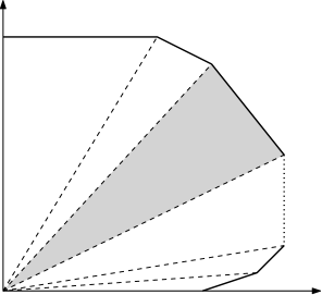
Figure 3: Schematic form of the polygon $\mathcal{P}_{n}$ for the $\widehat{D}_{n}$ quiver for a generic value of CS levels. Only the upper right quadrant is shown as it is symmetric along both the $x$ and $y$ axes.

The physical meaning of $\mathcal{P}_{n}$ was clarified in [27] (see also [28]) where an elegant Fermi gas approach was used to study the matrix model at finite $N$, showing that $\mathcal{P}_{n}$ corresponds to the Fermi surface of the system at large $N$, and confirming the proposal for the free energy of [16].

The goal for the rest of the paper is to derive (4.2) geometrically, by a direct computation of $\operatorname{Vol}(Y_{7})$ using the localization method of section 3. In order to do so, we must first identify the precise manifolds $Y_{7}$ dual to $\widehat{D}$–quivers, which we do next.

4.2 The Moduli Spaces

The manifold $Y_{7}$ dual to a certain CS quiver gauge theory can be found by analyzing the moduli space of the field theory [5, 6, 29], which is obtained by setting the $D$–terms and $F$–terms to zero, and modding out by the appropriate gauge transformations. Thus, we need to specify the superpotential $W$ appearing in (4.1). We can do this for a generic quiver. Consider a quiver with $n_{V}$ vertices corresponding to $U(n_{a}N)$ gauge groups (we assume all $n_{a}$ are coprime) and $n_{E}$ number of edges. Let us first set $N=1$. To determine the superpotential we follow the approach used in [5] by introducing an auxiliary chiral multiplet $Φ_{a}$ in the adjoint of the gauge group $a$ and superpotential $W_{a}=-\frac{n_{a}k_{a}}{2}Φ_{a}^{2}+\sum_{i\to a}A_{i}Φ_{a}B_{i}\,;$ here the sum is over all edges $i$ incident upon the node $a$ and $Φ_{a}=Φ_{a}^{A}T_{A}$, with $T_{A}$ the generators of the corresponding gauge group. To avoid cluttering the expressions we omit the gauge generators in what follows, but it should be clear where these sit. Since we will introduce a field $Φ_{a}$ for each node in the quiver it is convenient to introduce the notation $Φ\equiv(Φ_{1},\cdots,Φ_{n_{V}})^{{\sf T}}$ and $AB\equiv(A_{1}B_{1},\cdots,A_{n_{E}}B_{n_{E}})^{{\sf T}}$ for nodes and edges, respectively. The full superpotential then reads $W=\sum_{a}W_{a}=-\frac{1}{2}Φ^{{\sf T}}KΦ+Φ^{{\sf T}}{\cal I}\,AB$, where ${\cal I}$ is the oriented incidence matrix of the quiver and $K$ is a diagonal matrix with entries $K_{aa}=n_{a}k_{a}$. Since $Φ$ does not have a kinetic term it can be integrated out, leading to the superpotential

$$W=\tfrac{1}{2}(AB)^{{\sf T}}\,{\cal I}^{{\sf T}}K^{-1}{\cal I}\,AB\,.$$ (4.5)

We are now in a position to determine the exact geometry of the moduli space for a general CS quiver. Varying $W$ with respect to $A$ and factoring out a $B$ gives the $F$–term equations $(AB)^{{\sf T}}\,{\cal I}^{{\sf T}}K^{-1}{\cal I}=0$. The $D$–term equations are obtained by simply replacing $AB\textrightarrow|A|^{2}-|B|^{2}$. Combining $A$ and $\bar{B}$ into a quaternion $q$, these three real equations combine into the hyperkähler moment map equations $\sum_{j}Q^{i}_{j}(q_{j}^{\textdagger}(\sigma_{\alpha})q_{j})=0$, with $Q$ a charge matrix given by

$$Q={\cal I}^{{\sf T}}K^{-1}{\cal I}\,.$$ (4.6)

This fully characterizes the quotient manifold for generic ${\cal N}=3$ quivers. We now specialize this to $\widehat{D}_{n}$ quivers and begin with $\widehat{D}_{4}$ for simplicity.

$\boldsymbol{\widehat{D}_{4}}$.

Using the incidence matrix for $\widehat{D}_{4}$ the superpotential (4.5) reads

$$W=\frac{1}{2}\left[\sum_{i=1}^{4}\frac{1}{k_{i}}\left(A_{i}B_{i}A_{i}B_{i}\right)+\frac{1}{2k_{5}}\Bigg{(}∑_{i=1}^{4}B_{i}\cdot A_{i}\Bigg{)}\Bigg{(}∑_{j=1}^{4}B_{j}\cdot A_{j}\Bigg{)}\right],$$ (4.7)

where $(A\cdot B)^{2}\equiv(A\sigma_{A}B)(A\sigma_{A}B)$ and $\sigma_{A}=(I,\sigma_{a})$. Varying $W$ with respect to $A_{i}$ gives the $F$–term equations:

$$\frac{1}{k_{i}}B_{i}(A_{i}B_{i})+\frac{1}{2k_{5}}B_{i}(\sigma_{A})∑_{j=1}^{4}\left(B_{j}(\sigma_{A})A_{j}\right)=0\,.$$ (4.8)

Factoring out $B_{i}$, we have four matrix equations for each $i$. However, the $SU(2)$ part of the matrix gives the same equations for each $i$. In the quaternionic notation, all the $U(1)$ equations $\big{(}$from the $\sigma_{0}=I$ matrix in (4.8)$\big{)}$ can be combined into the single equation

$$∑_{j=1}^{4}Q^{i}_{j}(q_{j}^{\textdagger}(\sigma_{\alpha})q_{j})=0\qquad\text{with}\quad Q=\begin{pmatrix}k_{1}+2k_{5}&k_{1}&k_{1}&k_{1}\\ k_{2}&k_{2}+2k_{5}&k_{2}&k_{2}\\ k_{3}&k_{3}&k_{3}+2k_{5}&k_{3}\\ k_{4}&k_{4}&k_{4}&k_{4}+2k_{5}\end{pmatrix}.$$ (4.9)

Each column (lower index) in this matrix $Q$ represents a quaternion and each row (upper index) represents the $U(1)$ under which it is charged. This matrix can be obtained directly from (4.6); here we have multiplied each row ‘$i$’ by $2k_{i}k_{5}$ for convenience, which amounts to an unimportant rescaling of the corresponding vector multiplets. We note that this matrix has only four rows although the original number of $U(1)$’s is five. The reason for this is that an overall diagonal $U(1)$ is decoupled as nothing is charged under it and so this row has been removed. In addition, imposing the relation $k_{1}+k_{2}+k_{3}+k_{4}+2k_{5}=0$ one sees that rank$(Q)=3$ and hence another row must be removed (it does not matter which one) to obtain the final charge matrix. We have thus shown that the moduli space is given by the hyperkähler quotient ${\mathbb{H}}^{8}///SU(2)×U(1)^{3}$ with the action of the group on the quaternions determined by the matrix in (4.9).

$\boldsymbol{\widehat{D}_{n>4}}$.

The extension to $\widehat{D}_{n>4}$ quivers, with gauge group $U(2)^{n-3}×U(1)^{4}$, is direct. The superpotential (4.5) can be written as:

$$W=\frac{1}{2}\Bigg{[}\sum_{i=1}^{4}\frac{1}{k_{i}}\left(A_{i}B_{i}A_{i}B_{i}\right)+\frac{1}{2k_{5}}\left(A_{1}\cdot B_{1}+A_{2}\cdot B_{2}-A_{5}\cdot B_{5}\right)^{2}\\ +\frac{1}{2k_{n+1}}\left(A_{3}\cdot B_{3}+A_{4}\cdot B_{4}+A_{n}\cdot B_{n}\right)^{2}+\sum_{a=6}^{n}\frac{1}{2k_{a}}\left(A_{a-1}\cdot B_{a-1}-A_{a}\cdot B_{a}\right)^{2}\Bigg{]}.$$

Proceeding as above one concludes that the moduli space is given by the hyperkähler quotient (at zero level)

$${\cal C}\left(Y^{(n-3,n-1)}_{7}\right)={\mathbb{H}}^{4n-8}///SU(2)^{n-3}×U(1)^{n-1}\,,$$ (4.10)

with the action of the group on the quaternions given by the charge matrix (for $n>4$)

$$Q=\begin{pmatrix}k_{1}+2k_{5}&k_{1}&0&0&-k_{1}&0&0&0\\ k_{2}&k_{2}+2k_{5}&0&0&-k_{2}&0&0&0\\ 0&0&k_{3}+2k_{n+1}&k_{3}&0&\cdots&\cdots_{0}&k_{3}\\ 0&0&k_{4}&k_{4}+2k_{n+1}&0&\cdots&\cdots_{0}&k_{4}\\ -k_{6}&-k_{6}&0&0&k_{5}+k_{6}&-k_{5}&\ddots&0\\ 0&0&\vdots&\vdots&-k_{7}&k_{6}+k_{7}&\ddots_{k}&\ddots_{0}\\ 0&0&\vdots_{0}&\vdots_{0}&\ddots&\ddots_{k}&\ddots_{k+k}&-k_{n-1}\\ 0&0&k_{n}&k_{n}&\ddots_{0}&\ddots_{0}&-k_{n+1}&k_{n}+k_{n+1}\end{pmatrix}.$$ (4.11)

As above, the matrix is of rank $(n-1)$ after imposing $k_{1}+k_{2}+k_{3}+k_{4}+2(k_{5}+\cdots+k_{n+1})=0$ and one (any) row should be removed. This matrix can be obtained directly from (4.6); here we have multiplied each row by the lowest common denominator of all the (nonzero) entries in that row for convenience.

We note that while the quaternionic dimension of the resulting spaces (4.10) is two, there is only a single $U(1)$ remaining after the quotient and thus the spaces are non-toric. To see this, note that before gauging, the action for the $\widehat{D}_{n}$ quiver has a $U(1)^{n}$ global symmetry, acting on each quaternion as $U(1)_{i}\mathrel{\mathop{\ordinarycolon}}(A_{i},B_{i})\to(e^{\dot{\iota}\theta}A_{i},e^{-\dot{\iota}\theta}B_{i})$ for $i=1,\cdots,n$. As shown above, the gauging removes $(n-1)$ of them, leaving a single $U(1)$ in the quotient manifold. This is also the case for the $\widehat{E}$–quivers, as can be readily checked. For $\widehat{A}$–quivers, in contrast, there is initially a $U(1)^{n}$ symmetry but the quotient removes only $(n-2)$ of them, hence the moduli spaces are toric.

Since the moduli spaces are hyperkähler quotients of the form (3.1), with $d=2,s=n-3,r=n-1$, we may apply the localization formula (3.13) to compute their volumes, which we do next.

4.3 Volumes

We are now in position to compute the volumes of tri-Sasaki Einstein manifolds dual to $\widehat{D}$–quivers. For clarity of presentation, we sketch the basic steps for $\widehat{D}_{4}$ first and provide the details for general $\widehat{D}_{n>4}$ in Appendix A. Setting $d=2,s=1,r=3$ in (3.13) we have

$$\operatorname{Vol}\left(Y_{7}^{(1,3)}\right) =\frac{32}{3}∫_{0}^{∞}dφ\,φ^{2}\left(1+φ^{2}\right)∫_{-∞}^{∞}d^{3}ϕ∏_{±,a=1}^{4}\frac{1}{1+\big{(}φ±(Q_{a}^{i}ϕ_{i})\big{)}^{2}}\,·$$

To perform the $d^{3}\varphi$ integral it is convenient to use the Fourier transform identity

$$\frac{1}{[1+(φ+\varphi)^{2}][1+(φ-\varphi)^{2}]}=\frac{1}{4}\int\limits_{-\infty}^{\infty}dX\,\frac{e^{-|X|}}{2φ}\left(\frac{e^{-\dot{\iota}|X|φ}}{φ-\dot{\iota}}+\frac{e^{\dot{\iota}|X|φ}}{φ+\dot{\iota}}\right)e^{\dot{\iota}\varphi X}$$ (4.12)

for each term in $∏_{a=1}^{4}$. Performing the $d^{3}\varphi$ integrals generates $(2π)^{3}δ^{3}({\textstyle∑_{a}}Q^{i}_{a}X_{a})$, which can be integrated away by writing $X_{a}=k_{a}x$; it is directly checked from (4.9) that $∑_{a}Q_{a}^{i}k_{a}=0$. Thus, we obtain

$$\operatorname{Vol}\left(Y_{7}^{(1,3)}\right)=\frac{π^{3}}{3}∫_{-∞}^{∞}dx∫_{0}^{∞}dφ\,\frac{e^{-∑_{a}|k_{a}x|}}{φ^{2}(1+φ^{2})^{3}}∏_{a=1}^{4}\left[\frac{1}{2}\left(e^{-\dot{\iota}|k_{a}x|φ}(φ+\dot{\iota})+e^{\dot{\iota}|k_{a}x|φ}(φ-\dot{\iota})\right)\right].$$ (4.13)

We now perform the $φ$ integral by residues, converting $∫_{0}^{∞}dφ\textrightarrow\frac{1}{2}∫_{-∞}^{∞}dφ$ as the integrand is an even function of $φ$. We note that expanding the product of exponentials in (4.13) gives a total of sixteen terms and the precise integration contour in the complex plane needs to be chosen separately for each one. This is because the coefficient of $\dot{\iota}φ|x|$ in each term can be any one of the combinations $±|k_{1}|±|k_{2}|±|k_{3}|±|k_{4}|$. Thus, in order to decide how to close the contour at $∞$, we choose a particular ordering of $k$’s. It is convenient to go to the basis $k_{a}\textrightarrow α_{(a)}.p$ and order the $p$’s according to $p_{1}≥p_{2}≥p_{3}≥p_{4}≥0$ (this is simply a choice and one should repeat this for all possible orderings). This results in

$$\operatorname{Vol}\left(Y_{7}^{(1,3)}\right)=\frac{π^{4}}{3}\frac{1}{2}∫_{-∞}^{∞}dx\,e^{-2\left(p_{1}+p_{3}\right)|x|}\left[-\frac{1}{8}e^{-2\left(p_{1}-p_{3}\right)|x|}+\frac{1}{2}e^{-2(p_{2}-p_{3})|x|}\left(1+(p_{2}-p_{3})|x|\right)\right.\\ \left.-\frac{1}{8}\left(e^{-2(p_{2}-p_{4})|x|}+e^{-2(p_{2}+p_{4})|x|}\right)\right].$$ (4.14)

Finally, integrating over $x$ gives

$$\frac{\operatorname{Vol}\left(Y_{7}^{(1,3)}\right)}{\operatorname{Vol}\left(S^{7}\right)} =-\frac{1}{32p_{1}}+\frac{2p_{1}+3p_{2}-p_{3}}{8\left(p_{1}+p_{2}\right)^{2}}-\frac{1}{16(p_{1}+p_{2}+p_{3}-p_{4})}-\frac{1}{16\sum_{b=1}^{4}p_{b}}\,$$

$$=\frac{1}{2}∑_{a=0}^{4}\frac{γ_{a,a+1}}{\bar{\sigma}_{a}\bar{\sigma}_{a+1}}=\frac{1}{4}\text{Area}\left({\mathcal{P}}_{4}\right)\,,$$ (4.15)

where in the second line we used the definitions below (4.4) and the ordering of $p$’s we have chosen (one may check that the last line above gives the result of the integral for all possible orderings). Thus, we have shown that for $n=4$ one exactly reproduces the field theory prediction (4.2).

For generic $n\geq 4$ the volume formula reads

$$\begin{split}\frac{\operatorname{Vol}\left(Y_{7}^{(n-3,n-1)}\right)}{\operatorname{Vol}\left(S^{7}\right)}&=\frac{4^{2n-5}}{(π^{2})^{n-3}(2π)^{n-1}}∏_{i=1}^{n-3}∫_{0}^{∞}dφ_{i}(4πφ_{i}^{2})\big{(}1+φ_{i}^{2}\big{)}∏_{j=1}^{n-1}∫_{-∞}^{∞}dϕ_{j}\\ &\quad×∏_{±,a=1}^{2}\frac{1}{1+\big{(}φ_{1}±Q_{a}^{i}ϕ_{i}\big{)}^{2}}∏_{±,a=3}^{4}\frac{1}{1+\big{(}φ_{n-3}^{2}±Q_{a}^{i}ϕ_{i}\big{)}^{2}}\\ &\quad×∏_{±,a=5}^{n}\frac{1}{\left(1+(φ_{a-4}±φ_{a-3}±Q_{a}^{i}ϕ_{i})^{2}\right)}\,·\end{split}$$ (4.16)

The integrals can be performed by the same steps as in the $\widehat{D}_{4}$ case. Assuming the ordering $p_{1}≥p_{2}≥\cdots≥p_{n}≥0$ one finds (see Appendix A for details):

$$\frac{\operatorname{Vol}\left(Y_{7}^{(n-3,n-1)}\right)}{\operatorname{Vol}\left(S^{7}\right)} =\frac{1}{16}\sum_{a=1}^{n-3}\frac{c_{a}}{\sum_{b=1}^{a-1}p_{b}+(n-a-1)p_{a}}+\frac{2\sum_{b=1}^{n-3}p_{b}+3p_{n-2}-p_{n-1}}{8\left(\sum_{b=1}^{n-2}p_{b}\right)^{2}}$$

$$\qquad\quad-\frac{1}{16}\left(\frac{1}{\sum_{b=1}^{n-1}p_{b}-p_{n}}+\frac{1}{\sum_{b=1}^{n}p_{b}}\right)$$

$$=\frac{1}{4}\text{Area}(\mathcal{P}_{n})\,,$$ (4.17)

in perfect agreement with the field theory prediction (4.2)!

5 Summary and Outlook

This paper contains two main results. The first is an explicit integral formula computing the volumes of tri-Sasaki Einstein manifolds given by nonabelian hyperkähler quotients. This is a generalization of the formula derived by Yee [21] in the Abelian case. The second result concerns the study of 3d ${\cal N}=3$ CS matter theories. We identified the precise (non-toric) tri-Sasaki Einstein manifolds describing the gravity duals of $\widehat{D}$–quivers and computed their volumes, showing perfect agreement with the field theory prediction of [16]. This greatly expands the detailed tests of AdS₄/CFT₃ available for non-toric cases.

One may also consider CS $\widehat{E}$–quivers, whose free energies were computed in [16]. In this case the corresponding hyperkähler quotients are $\widehat{E}_{6}\mathrel{\mathop{\ordinarycolon}}\,\mathbb{H}^{24}///SU(3)\times SU(2)^{3}\times U(1)^{5}$, $\widehat{E}_{7}\mathrel{\mathop{\ordinarycolon}}\,\mathbb{H}^{48}///SU(4)\times SU(3)^{2}\times SU(2)^{3}\times U(1)^{6}$, and $\widehat{E}_{8}\mathrel{\mathop{\ordinarycolon}}\,\mathbb{H}^{120}///SU(6)\times SU(5)\times SU(4)^{2}\times SU(3)^{2}\times SU(2)^{2}\times U(1)^{7}$. The volume integrals can be written using (3.16) and the relevant charge matrices (4.6). Although we have not computed these integrals explicitly one should be able to do so with the same techniques used here for $\widehat{D}$–quivers. An open question regarding $\widehat{E}$–quivers is whether they admit a Fermi gas description, along the lines of [30] for $\widehat{A}$–quivers and [27, 28] for $\widehat{D}$–quivers. If so, the integral volume formula may elucidate the form of the Fermi surface in the large $N$ limit.

The localization approach can also be applied to nonabelian Kähler quotients. This is the relevant setting for AdS₅/CFT₄, where few non-toric examples are known. An important distinction, however, is that the quotient ensures only the Kähler class of the quotient manifold and not its metric structure. In this case one would have to combine this approach with the principle of volume minimization, along the lines of [24, 23]. It is our hope that the formulas presented here will also be valuable in this context.

Finally, one may also consider quivers whose nodes represent $SO(N)$ or $USp(2N)$ gauge groups. Related to this, it may be interesting to consider the interplay of the volume formulas with the folding/unfolding procedure of [31].

Appendix A $\boldsymbol{\widehat{D}_{n}}$ CS Quivers

Here we provide the details leading to the main result for CS $\widehat{D}_{n}$ quivers (4.17). For generic $n$ the volume formula reads:

$$\operatorname{Vol}\left(Y_{7}^{(n-3,n-1)}\right) =\left(\frac{π^{4}}{3}\right)\frac{4^{2n-5}}{(π^{2})^{n-3}(2π)^{n-1}}∏_{i=1}^{n-3}∫_{0}^{∞}dφ_{i}(4πφ_{i}^{2})\big{(}1+φ_{i}^{2}\big{)}∏_{j=1}^{n-1}∫_{-∞}^{∞}dϕ_{j}$$

$$\quad×∏_{±,a=1}^{2}\frac{1}{1+\big{(}φ_{1}±Q_{a}^{i}ϕ_{i}\big{)}^{2}}∏_{±,a=3}^{4}\frac{1}{1+\big{(}φ_{n-3}^{2}±Q_{a}^{i}ϕ_{i}\big{)}^{2}}$$

$$\quad×∏_{±,a=5}^{n}\frac{1}{\left(1+(φ_{a-4}±φ_{a-3}±Q_{a}^{i}ϕ_{i})^{2}\right)}\,·$$ (A.1)

The basic procedure follows the same logic of the $\widehat{D}_{4}$ case. We first exponentiate the denominators by introducing some $∫dy_{a}$’s, perform the $ϕ$–integrals to generate $δ(∑_{a}Q^{i}_{a}y_{a})$–functions, and solve the equations $∑_{a}Q^{i}_{a}y_{a}=0$ by $y_{a}=κ_{a}x$ such that $∑_{a}Q^{i}_{a}κ_{a}=0$ where $κ_{a}=\{p_{1}+p_{2},p_{1}-p_{2},p_{n-1}-p_{n},p_{n-1}+p_{n},2p_{3},2p_{4},⋯,2p_{n-2}\}$ (up to some signs but since only $|κ_{a}|$ are needed below these are not important). Now, assuming

$$p_{1}≥p_{2}≥\cdots≥p_{n}≥0\,,$$ (A.2)

all $κ_{a}\geq 0$ and thus we may replace $|κ_{a}|\to κ_{a}$. Next, we perform all the $y_{a}$ integrals obtaining

$$\frac{\operatorname{Vol}\left(Y_{7}^{(n-3,n-1)}\right)}{\operatorname{Vol}\left(S^{7}\right)}=\frac{4^{2n-5}4^{n-3}}{π^{n-3}}\frac{1}{4^{4}}\frac{1}{32^{n-4}}∫_{-∞}^{∞}dx\,e^{-∑_{a=1}^{n}κ_{a}|x|}∏_{i=1}^{n-3}∫_{0}^{∞}dφ_{i}\,φ_{i}^{2}\big{(}1+φ_{i}^{2}\big{)}\\ ×∏_{a=1}^{2}{\cal D}_{κ_{a}}(φ_{1},x)∏_{a=3}^{4}{\cal D}_{κ_{a}}(φ_{n-3},x)∏_{a=5}^{n}{\cal D}_{κ_{a}}(φ_{a-4},φ_{a-3},x)\,,$$ (A.3)

where

$$\begin{aligned} {\cal D}_{κ_{a}}(φ_{i},x)&=\frac{φ_{i}\cos(φ_{i}κ_{a}|x|)+\sin(φ_{i}κ_{a}|x|)}{φ_{i}(1+φ_{i}^{2})}\\ {\cal D}_{κ_{a}}(φ_{i},φ_{j},x)&=\frac{\left[\begin{array}[]{c}φ_{i}φ_{j}(φ_{i}^{2}-φ_{j}^{2})(5+φ_{i}^{2}+φ_{j}^{2})\cos(φ_{i}κ_{a}|x|)\cos(φ_{j}κ_{a}|x|)\\ +2(1+φ_{i}^{2})(1+φ_{j}^{2})(φ_{i}^{2}-φ_{j}^{2})\sin(φ_{i}κ_{a}|x|)\sin(φ_{j}κ_{a}|x|)\\ -φ_{i}(1+φ_{i}^{2})(1-φ_{i}^{2}+5φ_{j}^{2})\cos(φ_{i}κ_{a}|x|)\sin(φ_{j}κ_{a}|x|)\\ +φ_{j}(1+φ_{j}^{2})(1+5φ_{i}^{2}-φ_{j}^{2})\sin(φ_{i}κ_{a}|x|)\cos(φ_{j}κ_{a}|x|)\end{array}\right]}{φ_{i}φ_{j}(φ_{i}^{2}-φ_{j}^{2})(1+φ_{i}^{2})(1+φ_{j}^{2})(1+(φ_{i}+φ_{j})^{2})(1+(φ_{i}-φ_{j})^{2})}\,·\end{aligned}$$ (A.4)

By performing the integrals in decreasing order of $φ$’s, starting from $φ_{n-3},⋯,φ_{1}$ a pattern emerges. Here are a few intermediate steps:

$${\cal I}_{n-3}=∫dφ_{n-3}\,φ_{n-3}^{2}\big{(}1+φ_{n-3}^{2}\big{)}∏_{a=3}^{4}{\cal D}_{κ_{a}}(φ_{n-3},x){\cal D}_{κ_{n}}(φ_{n-4},φ_{n-3},x)=\frac{π}{2}∏_{a=3}^{4}{\cal D}_{κ_{a}}(φ_{n-4},x)\\ +\frac{π}{4}e^{2(-p_{n-2}+p_{n-1})|x|}\frac{φ_{n-4}(φ_{n-4}^{2}-5)\cos(φ_{n-4}κ_{n}|x|)+2(2φ_{n-4}^{2}-1)\sin(φ_{n-4}κ_{n}|x|)}{φ_{n-4}(1+φ_{n-4}^{2})^{2}(4+φ_{n-4}^{2})}\,·$$ (A.5)

Let us define another ${\cal D}$ to keep the expressions relatively compact:

$${\cal D}_{κ_{a}}(φ_{i},x;\mathfrak{m})=\frac{φ_{i}\left(φ_{i}^{2}-\mathfrak{m}(\mathfrak{m}+1)+1\right)\cos(φ_{i}κ_{a}|x|)+\mathfrak{m}(2φ_{i}^{2}-\mathfrak{m}+1)\sin(φ_{i}κ_{n}|x|)}{φ_{i}\left(1+φ_{i}^{2}\right)\left((\mathfrak{m}-1)^{2}+φ_{i}^{2}\right)\left(\mathfrak{m}^{2}+φ_{i}^{2}\right)}\,·$$ (A.6)

Thus the relevant expression in (A.5) can be labelled ${\cal D}_{κ_{n}}(φ_{n-4},x;2)$. Proceeding further with the integrals we have

$${\cal I}_{n-3>j>1}=∫dφ_{j}\,φ_{j}^{2}\big{(}1+φ_{j}^{2}\big{)}{\cal D}_{κ_{j+3}}(φ_{j-1},φ_{j},x)\,{\cal I}_{j+1}\\ =\left(\frac{π}{2}\right)^{n-2-j}\left[∏_{a=3}^{4}{\cal D}_{κ_{a}}(φ_{j-1},x)+\frac{1}{2}∑^{a=n}_{j+3}e^{-2\left((n-a+1)p_{a-2}-∑_{b=a-1}^{n-1}p_{b}\right)|x|}{\cal D}_{κ_{a}}(φ_{j-1},x;n-a+2)\right].$$ (A.7)

The final $φ_{1}$–integral then gives

$${\cal I}_{1} =∫dφ_{1}\,φ_{1}^{2}\big{(}1+φ_{1}^{2}\big{)}∏_{a=1}^{2}{\cal D}_{κ_{a}}(φ_{1},x)\,{\cal I}_{2}$$

$$=\left(\frac{π}{2}\right)^{n-3}\left[\frac{c_{1}}{8}e^{-2\left((n-3)p_{1}-∑_{b=3}^{n-1}p_{b}\right)|x|}+∑_{a=2}^{n-3}\frac{c_{a}}{8}e^{-2\left(∑_{b=2}^{a-1}p_{b}+(n-a-1)p_{a}-∑_{b=3}^{n-1}p_{b}\right)|x|}\right.$$

$$\quad\left.+\frac{1}{2}e^{-2(p_{2}-p_{n-1})|x|}\left(1+(p_{n-2}-p_{n-1})|x|\right)-\frac{1}{8}\left(e^{-2(p_{2}-p_{n})|x|}+e^{-2(p_{2}+p_{n})|x|}\right)\right],$$ (A.8)

where $c_{a}=\frac{-2}{(n-a-1)(n-a-2)}$. This expression is also valid for $\widehat{D}_{4}$, as can be easily checked.

Finally, performing the integral over $x$ gives

$$\frac{\operatorname{Vol}\left(Y_{7}^{(n-3,n-1)}\right)}{\operatorname{Vol}\left(S^{7}\right)} =\frac{2^{n-4}}{π^{n-3}}∫_{-∞}^{∞}dx\,e^{-2\left(p_{1}+∑_{b=3}^{n-1}p_{b}\right)|x|}\;{\cal I}_{1}$$

$$=\frac{1}{16}\sum_{a=1}^{n-3}\frac{c_{a}}{\sum_{b=1}^{a-1}p_{b}+(n-a-1)p_{a}}+\frac{2\sum_{b=1}^{n-3}p_{b}+3p_{n-2}-p_{n-1}}{8\left(\sum_{b=1}^{n-2}p_{b}\right)^{2}}$$

$$\quad-\frac{1}{16}\left(\frac{1}{\sum_{b=1}^{n-1}p_{b}-p_{n}}+\frac{1}{\sum_{b=1}^{n}p_{b}}\right)·$$ (A.9)

The expression appearing on the right hand side of (A) is precisely the area of the polygon (4.3) (see [16] for details). Indeed, using the definitions below (4.4) and the ordering (A.2), this becomes

$$\frac{\operatorname{Vol}\left(Y_{7}^{(n-3,n-1)}\right)}{\operatorname{Vol}\left(S^{7}\right)}=\frac{1}{2}∑_{a=0}^{n}\frac{γ_{a,a+1}}{\bar{\sigma}_{a}\bar{\sigma}_{a+1}}=\frac{1}{4}\text{Area}({\mathcal{P}}_{n})\,,$$

as we wanted to show.

Appendix B Other Examples

In this Appendix we provide other examples of applications of the formula (3.13).

B.1 A Lindström-Roček Space

Consider a Lindström-Roček Space [32] given by the hyperkähler quotient ${\mathbb{H}}^{6}///U(2)$. This amounts to setting $d=2,s=1,r=1$ in (3.13) and the volume reads

$$\operatorname{Vol}\left(Y^{(1,1)}_{7}\right) =\frac{32π^{4}}{6[(π^{2})(2π)]}∫_{0}^{∞}dφ(4πφ^{2})\left(1+φ^{2}\right)∫_{-∞}^{∞}dϕ\frac{1}{\left(1+2\big{(}φ^{2}+ϕ^{2}\big{)}+\big{(}φ^{2}-ϕ^{2}\big{)}^{2}\right)^{3}}$$

$$=\frac{32π^{2}}{3}∫_{0}^{∞}dφ\,φ^{2}\left(1+φ^{2}\right)\left[\frac{3π(21+6φ^{2}+φ^{4})}{256\left(1+φ^{2}\right)^{5}}\right]$$

$$=\frac{π^{3}}{8}∫_{0}^{∞}dφ\,\frac{φ^{2}(21+6φ^{2}+φ^{4})}{\left(1+φ^{2}\right)^{4}}=\frac{π^{4}}{8}\,·$$

One can verify that this is the correct value by explicit construction of the hyperkähler potential. Following [32], the hyperkähler cone ${\mathbb{H}}^{6}///U(2)$ is described by the following action (with all FI parameters vanishing)

$$S=∫d^{8}z\left[\bar{Φ}_{a+}^{m}\big{(}e^{V}\big{)}^{a}_{b}Φ^{b}_{m+}+Φ^{m}_{a-}\big{(}e^{-V}\big{)}^{a}_{b}\bar{Φ}^{b}_{m-}\right]+\left[∫d^{6}zΦ^{b}_{m+}S_{b}^{a}Φ^{m}_{a-}+h.c.\right].$$ (B.1)

Here, $m=1,2,3$ and $a=1,2$ is the $U(2)$ index. This gives the following equations of motion

$$Φ^{b}_{m+}\bar{Φ}^{m}_{a+}\big{(}e^{V}\big{)}^{a}_{b}-\big{(}e^{-V}\big{)}^{a}_{b}\bar{Φ}^{b}_{m-}Φ^{m}_{a-} =0$$ (B.2)

$$Φ^{b}_{m+}Φ^{m}_{a-} =0\,.$$ (B.3)

Solving the latter equation by

$$Φ^{a}_{+} =\left(K^{a}_{+},\frac{\dot{\iota}K_{1-}K^{a}_{+}}{\sqrt{K^{a}_{+}K_{a-}}},\frac{\dot{\iota}K_{2-}K^{a}_{+}}{\sqrt{K^{a}_{+}K_{a-}}}\right)$$ (B.4)

$$Φ_{a-} =\left(K_{a-},\frac{\dot{\iota}K_{a-}K^{1}_{+}}{\sqrt{K^{a}_{+}K_{a-}}},\frac{\dot{\iota}K_{a-}K^{2}_{+}}{\sqrt{K^{a}_{+}K_{a-}}}\right)^{\!\!{\sf T}},$$ (B.5)

where we have chosen a particular gauge, and plugging the solution for $e^{V}$ back in (B.1) leads to the action

$$S =\operatorname{Tr}∫d^{8}z\sqrt{4Φ^{b}_{m+}\bar{Φ}^{m}_{c+}\bar{Φ}^{c}_{m-}Φ^{m}_{a-}}$$

$$=2∫d^{8}z\sqrt{\left(K^{1}_{+}\bar{K}_{1+}+K^{2}_{+}\bar{K}_{2+}+κ\right)\left(K_{1-}\bar{K}^{1}_{-}+K_{2-}\bar{K}^{2}_{-}+κ\right)}\,,$$ (B.6)

where $κ^{2}=(K^{1}_{+}K_{1-}+K^{2}_{+}K_{2-})(\bar{K}^{1}_{+}\bar{K}_{1-}+\bar{K}^{2}_{+}\bar{K}_{2-})$. The metric is given by $g_{i\bar{j}}=∂_{i\bar{j}}{\cal K}$ where Kähler potential ${\cal K}$ is obtained from $S=∫d^{8}z{\cal K}$. It turns out that

$$g≡\det g_{i\bar{j}}=2^{8}.$$ (B.7)

We use the following coordinate transformation to spherical polar coordinates

$$\begin{aligned} K^{1}_{+}&=r\cos χ\cos\tfrac{θ_{1}}{2}e^{\frac{\dot{\iota}}{2}(-φ_{1}+2ψ_{1})}\\ K_{1-}&=r\cos χ\sin\tfrac{θ_{1}}{2}e^{\frac{\dot{\iota}}{2}(-φ_{1}-2ψ_{1})}\\ K^{2}_{+}&=r\sin χ\cos\tfrac{θ_{2}}{2}e^{\frac{\dot{\iota}}{2}(-φ_{2}+2ψ_{2})}\\ K_{2-}&=r\sin χ\sin\tfrac{θ_{2}}{2}e^{\frac{\dot{\iota}}{2}(-φ_{2}-2ψ_{2})}\,.\end{aligned}$$ (B.8)

Here, $r$ is the radial coordinate and $θ_{i},φ_{i},ψ_{i}$ are the usual 3D spherical coordinates so $θ_{i}\in[0,π]$, $φ_{i}\in[0,2π)$ and $ψ_{i}\in[0,2π)$. The limit of $χ\in[0,\frac{π}{2}]$ is chosen such that the ‘flat’ action gives flat metric on $R_{+}×S⁷$. The determinant of the Jacobian of this transformation is

$$J_{s}=r^{7}\cos^{3}χ\sin^{3}χ\sin θ_{1}\sin θ_{2}.$$ (B.9)

In these coordinates the metric is not explicitly conical (there are off-diagonal terms between $dr$ and spherical coordinates) but $g_{rr}$ is a complicated function of spherical coordinates only and rescaling $r\textrightarrow\frac{ρ}{\sqrt{g_{rr}}}$ one obtains the conical metric $dρ^{2}+ρ^{2}dΩ_{7}^{2}$. The determinant of this radial transformation is

$$J_{r}=\frac{1}{\sqrt{g_{rr}}}\,·$$ (B.10)

Combining all the above determinants, taking square root and (numerically) integrating over the spherical coordinates gives us the volume of the seven-dimensional base of the hyperkähler cone:

$$\operatorname{Vol}(Ω_{7})=∫_{Ω_{7}}\sqrt{g}\,J_{s}\,J_{r}|_{ρ\textrightarrow 1}=∫_{Ω_{7}}\frac{16\cos^{3}χ\sin^{3}χ\sin θ_{1}\sin θ_{2}}{g_{rr}^{4}}=\frac{π^{4}}{8}\,·$$ (B.11)

B.2 Volume of $\boldsymbol{{\mathbb{D}}}$–orbifolded $\boldsymbol{S^{3}}$

Here we provide details of the calculation for ALE instantons of section 3.1 for generic $\mathbb{D}_{k-2}$. The volume integral reads:

$$\operatorname{Vol}\left(Y^{(k-3,k)}_{3}\right) =\frac{2^{3(k-3)+k+1}π^{2}}{(π^{2})^{k-3}×(2π)^{k}}∫∏_{i=1}^{k-3}dφ_{i}\left(4πφ_{i}^{2}\right)\left(1+φ_{i}^{2}\right)∏_{j=1}^{k}dϕ_{j}\,∏_{±}\frac{1}{1+\left(φ_{1}±ϕ_{4}\right)^{2}}$$

$$\quad×∏_{±}\frac{1}{1+\left(φ_{1}±(ϕ_{1}+ϕ_{4})\right)^{2}}∏_{±,a=2}^{3}\frac{1}{1+\left(φ_{k-3}±(ϕ_{a}+ϕ_{k})\right)^{2}}$$

$$\quad×∏_{±,a=1}^{k-4}\frac{1}{1+\left((φ_{a}±φ_{a+1})±(ϕ_{a+3}-ϕ_{a+4})\right)^{2}}\,·$$ (B.12)

Using Fourier transform to exponentiate all the denominators, we obtain

$$\operatorname{Vol}\left(Y^{(k-3,k)}_{3}\right) =\frac{2^{5k-14}}{π^{2k-5}}∫∏_{i=1}^{k-3}dφ_{i}\,φ_{i}^{2}\left(1+φ_{i}^{2}\right)∏_{j=1}^{k}dϕ_{j}∏_{±,a=1}^{4}dy_{a}^{±}∏_{±,b=1}^{k-4}dη_{b}^{±}d\bar{η}_{b}^{±}$$

$$\quad×\left(\tfrac{1}{2}\right)^{8}e^{-∑_{±,a=1}^{4}|y_{a}^{±}|+\dot{\iota}∑_{±}\left(y_{1}^{±}(φ_{1}±ϕ_{4})+y_{2}^{±}\left(φ_{1}±(ϕ_{1}+ϕ_{4})\right)+∑_{a=2}^{3}y_{a+1}^{±}\left(φ_{k-3}±(ϕ_{a}+ϕ_{k})\right)\right)}$$

$$\quad×\left(\tfrac{1}{2}\right)^{4(k-4)}e^{∑_{±,b=1}^{k-4}\left(\!-|η_{b}^{±}|+\dot{\iota}η_{b}^{±}\left(\!(φ_{b}+φ_{b+1})±(ϕ_{b+3}-ϕ_{b+4})\!\right)-|\bar{η}_{b}^{±}|+\dot{\iota}\bar{η}_{b}^{±}\left(\!(φ_{b}-φ_{b+1})±(ϕ_{b+3}-ϕ_{b+4})\!\right)\!\right)}$$

$$=\frac{2^{k-6}}{π^{2k-5}}∫∏_{i=1}^{k-3}dφ_{i}\,φ_{i}^{2}\left(1+φ_{i}^{2}\right)∏_{j=1}^{k}dϕ_{j}∏_{±,a=1}^{4}dy_{a}^{±}∏_{±,b=1}^{k-4}dη_{b}^{±}d\bar{η}_{b}^{±}$$

$$\quad×e^{-∑_{±,a=1}^{4}|y_{a}^{±}|-∑_{±,b=1}^{k-4}\left(|η_{b}^{±}|+|\bar{η}_{b}^{±}|\right)}\,e^{\dot{\iota}∑_{±}\left(φ_{1}\left(y_{1}^{±}+y_{2}^{±}\right)+φ_{k-3}\left(y_{3}^{±}+y_{4}^{±}\right)\right)}$$

$$\quad×e^{\dot{\iota}∑_{a=1}^{3}ϕ_{a}\left(y_{a+1}^{+}-y_{a+1}^{-}\right)+\dot{\iota}ϕ_{4}\left(y_{1}^{+}-y_{1}^{-}+y_{2}^{+}-y_{2}^{-}\right)+\dot{\iota}ϕ_{k}\left(y_{3}^{+}-y_{3}^{-}+y_{4}^{+}-y_{4}^{-}\right)}$$

$$\quad×e^{\dot{\iota}φ_{1}\left(η_{1}^{+}+η_{1}^{-}+\bar{η}_{1}^{+}+\bar{η}_{1}^{-}\right)+\dot{\iota}φ_{k-3}\left(η_{k-4}^{+}+η_{k-4}^{-}-\bar{η}_{k-4}^{+}-\bar{η}_{k-4}^{-}\right)+\dot{\iota}∑_{±,b=2}^{k-4}φ_{b}\left(η_{b-1}^{±}-\bar{η}_{b-1}^{±}+η_{b}^{±}+\bar{η}_{b}^{±}\right)}$$

$$\quad×e^{\dot{\iota}ϕ_{4}\left(η_{1}^{+}-η_{1}^{-}+\bar{η}_{1}^{+}-\bar{η}_{1}^{-}\right)-\dot{\iota}ϕ_{k}\left(η_{k-4}^{+}-η_{k-4}^{-}+\bar{η}_{k-4}^{+}-\bar{η}_{k-4}^{-}\right)+\dot{\iota}∑_{±,b=2}^{k-4}ϕ_{b+3}\left(∓η_{b-1}^{±}∓\bar{η}_{b-1}^{±}±η_{b}^{±}±\bar{η}_{b}^{±}\right)}\,.$$

We can perform the three $ϕ_{a},a=1,2,3$ integrals to generate three $δ$–functions, which can be used to do $y_{a}^{-},a=2,3,4$ integrals as follows:

$$\operatorname{Vol}\left(Y^{(k-3,k)}_{3}\right) =\frac{2^{k-6}}{π^{2k-5}}∫∏_{i=1}^{k-3}dφ_{i}\,φ_{i}^{2}\left(1+φ_{i}^{2}\right)∏_{j=4}^{k}dϕ_{j}∏_{a=1}^{4}dy_{a}^{+}dy_{1}^{-}∏_{±,b=1}^{k-4}dη_{b}^{±}d\bar{η}_{b}^{±}$$

$$\quad×e^{-∑_{±}|y_{1}^{±}|-2∑_{a=2}^{4}|y_{a}^{+}|-∑_{±,b=1}^{k-4}\left(|η_{b}^{±}|+|\bar{η}_{b}^{±}|\right)}\,e^{\dot{\iota}\left(φ_{1}\left(y_{1}^{+}+y_{1}^{-}+2y_{2}^{+}\right)+2φ_{k-3}\left(y_{3}^{+}+y_{4}^{+}\right)\right)}$$

$$\quad×e^{\dot{\iota}φ_{1}\left(η_{1}^{+}+η_{1}^{-}+\bar{η}_{1}^{+}+\bar{η}_{1}^{-}\right)+\dot{\iota}φ_{k-3}\left(η_{k-4}^{+}+η_{k-4}^{-}-\bar{η}_{k-4}^{+}-\bar{η}_{k-4}^{-}\right)+\dot{\iota}∑_{±,b=2}^{k-4}φ_{b}\left(η_{b-1}^{±}-\bar{η}_{b-1}^{±}+η_{b}^{±}+\bar{η}_{b}^{±}\right)}$$

$$\quad×(2π)^{3}e^{\dot{\iota}ϕ_{4}\left(y_{1}^{+}-y_{1}^{-}\right)}e^{\dot{\iota}ϕ_{4}\left(η_{1}^{+}-η_{1}^{-}+\bar{η}_{1}^{+}-\bar{η}_{1}^{-}\right)-\dot{\iota}ϕ_{k}\left(η_{k-4}^{+}-η_{k-4}^{-}+\bar{η}_{k-4}^{+}-\bar{η}_{k-4}^{-}\right)}$$

$$\quad×e^{\dot{\iota}∑_{±,b=2}^{k-4}ϕ_{b+3}\left(∓η_{b-1}^{±}∓\bar{η}_{b-1}^{±}±η_{b}^{±}±\bar{η}_{b}^{±}\right)}\,.$$

This form now shows that all the remaining $ϕ$–integrals can be done similarly to generate more $δ$–functions involving $η$’s and then all the remaining $y^{+}$ and $η^{±}$-integrals can be performed, leaving only the $φ$–integrals.

$$\operatorname{Vol}\left(Y^{(k-3,k)}_{3}\right) =\frac{2^{k-6}}{π^{2k-5}}(2π)^{k}∫∏_{i=1}^{k-3}dφ_{i}\,φ_{i}^{2}\left(1+φ_{i}^{2}\right)∏_{a=1}^{4}dy_{a}^{+}∏_{±,b=1}^{k-4}dη_{b}^{±}d\bar{η}_{b}^{±}\,e^{-2∑_{a=1}^{4}|y_{a}^{+}|}$$

$$\quad×e^{2\dot{\iota}\left(φ_{1}\left(y_{1}^{+}+y_{2}^{+}\right)+φ_{k-3}\left(y_{3}^{+}+y_{4}^{+}\right)\right)}∏_{b=1}^{k-4}δ\left(η_{b}^{+}-η_{b}^{-}+\bar{η}_{b}^{+}-\bar{η}_{b}^{-}\right)e^{-∑_{±,b=1}^{k-4}\left(|η_{b}^{±}|+|\bar{η}_{b}^{±}|\right)}$$

$$\quad×e^{\dot{\iota}φ_{1}\left(η_{1}^{+}+η_{1}^{-}+\bar{η}_{1}^{+}+\bar{η}_{1}^{-}\right)+\dot{\iota}φ_{k-3}\left(η_{k-4}^{+}+η_{k-4}^{-}-\bar{η}_{k-4}^{+}-\bar{η}_{k-4}^{-}\right)+\dot{\iota}∑_{±,b=2}^{k-4}φ_{b}\left(η_{b-1}^{±}-\bar{η}_{b-1}^{±}+η_{b}^{±}+\bar{η}_{b}^{±}\right)}$$

$$=\frac{2^{2k-6}}{π^{k-5}}∫∏_{i=1}^{k-3}dφ_{i}\,\frac{φ_{i}^{2}\left(1+φ_{i}^{2}\right)}{\left(1+φ_{1}^{2}\right)^{2}\left(1+φ_{k-3}^{2}\right)^{2}}∏_{±,b=1}^{k-4}dη_{b}^{±}d\bar{η}_{b}^{+}$$

$$\quad×e^{-∑_{b=1}^{k-4}\left(|η_{b}^{+}|+|η_{b}^{-}|+|\bar{η}_{b}^{+}|+|η_{b}^{+}-η_{b}^{-}+\bar{η}_{b}^{+}|\right)}$$

$$\quad×e^{2\dot{\iota}φ_{1}\left(η_{1}^{+}+\bar{η}_{1}^{+}\right)+2\dot{\iota}φ_{k-3}\left(η_{k-4}^{-}-\bar{η}_{k-4}^{+}\right)+2\dot{\iota}∑_{b=2}^{k-4}φ_{b}\left(η_{b-1}^{-}-\bar{η}_{b-1}^{+}+η_{b}^{+}+\bar{η}_{b}^{+}\right)}$$

$$=\frac{2^{2k-6}}{π^{k-5}}∫∏_{i=1}^{k-3}dφ_{i}\,\frac{φ_{i}^{2}\left(1+φ_{i}^{2}\right)}{\left(1+φ_{1}^{2}\right)^{2}\left(1+φ_{k-3}^{2}\right)^{2}}$$

$$\quad×∏_{b=1}^{k-4}\frac{5+φ_{b}^{2}+φ_{b+1}^{2}}{2(1+φ_{b}^{2})(1+φ_{b+1}^{2})(1+(φ_{b}+φ_{b+1})^{2})(1+(φ_{b}-φ_{b+1})^{2})}$$

$$=\frac{2^{k-2}}{π^{k-5}}∫∏_{i=1}^{k-3}dφ_{i}\,\frac{φ_{i}^{2}}{(1+φ_{1}^{2})^{2}(1+φ_{k-3}^{2})}$$

$$\quad×∏_{b=1}^{k-4}\frac{5+φ_{b}^{2}+φ_{b+1}^{2}}{(1+φ_{b+1}^{2})(1+(φ_{b}+φ_{b+1})^{2})(1+(φ_{b}-φ_{b+1})^{2})}\,·$$

Finally, performing all the $φ$–integrals one-by-one with the residue algorithm used in the main text (and Appendix A), we get

$$\operatorname{Vol}\left(Y^{(k-3,k)}_{3}\right) =\frac{{2^{k-2}}}{π^{k-5}}\frac{π}{{4}\left(1+(k-3)\right)^{2}}∏_{a=1}^{k-4}\frac{(a+2)π}{{2}(a+1)}$$

$$=\frac{π^{2}}{2(k-2)}\,,$$ (B.13)

as expected.

References

- [1] I. R. Klebanov and E. Witten, “Superconformal Field Theory on Three-branes at a Calabi-Yau Singularity,” Nucl. Phys. B536 (1998) 199–218, arXiv:hep-th/9807080.
- [2] J. P. Gauntlett, D. Martelli, J. Sparks, and D. Waldram, “Sasaki-Einstein Metrics on ,” Adv. Theor. Math. Phys. 8 (2004) 711–734, arXiv:hep-th/0403002.
- [3] D. Martelli and J. Sparks, “Toric Geometry, Sasaki-Einstein Manifolds and a New Infinite Class of AdS/CFT Duals,” Commun. Math. Phys. 262 (2006) 51–89, arXiv:hep-th/0411238.
- [4] S. Benvenuti, S. Franco, A. Hanany, D. Martelli, and J. Sparks, “An Infinite Family of Superconformal Quiver Gauge Theories with Sasaki-Einstein Duals,” JHEP 06 (2005) 064, arXiv:hep-th/0411264.
- [5] O. Aharony, O. Bergman, D. L. Jafferis, and J. Maldacena, “ Superconformal Chern-Simons-Matter Theories, M2-branes and their Gravity Duals,” JHEP 10 (2008) 091, arXiv:0806.1218 [hep-th].
- [6] D. L. Jafferis and A. Tomasiello, “A Simple Class of Gauge/Gravity Duals,” JHEP 10 (2008) 101, arXiv:0808.0864 [hep-th].
- [7] C. P. Herzog, I. R. Klebanov, S. S. Pufu, and T. Tesileanu, “Multi-Matrix Models and Tri-Sasaki Einstein Spaces,” Phys. Rev. D83 (2011) 046001, arXiv:1011.5487 [hep-th].
- [8] D. R. Gulotta, C. P. Herzog, and S. S. Pufu, “From Necklace Quivers to the F-theorem, Operator Counting, and ,” JHEP 12 (2011) 077, arXiv:1105.2817 [hep-th].
- [9] D. L. Jafferis, I. R. Klebanov, S. S. Pufu, and B. R. Safdi, “Towards the F-Theorem: Field Theories on the Three-Sphere,” JHEP 06 (2011) 102, arXiv:1103.1181 [hep-th].
- [10] A. Amariti, C. Klare, and M. Siani, “The Large– Limit of Toric Chern-Simons Matter Theories and Their Duals,” JHEP 10 (2012) 019, arXiv:1111.1723 [hep-th].
- [11] D. Martelli and J. Sparks, “The Large– Limit of Quiver Matrix Models and Sasaki-Einstein Manifolds,” Phys. Rev. D84 (2011) 046008, arXiv:1102.5289 [hep-th].
- [12] N. Drukker, M. Mariño, and P. Putrov, “From Weak to Strong Coupling in ABJM Theory,” Commun. Math. Phys. 306 (2011) 511–563, arXiv:1007.3837 [hep-th].
- [13] A. Kapustin, B. Willett, and I. Yaakov, “Exact Results for Wilson Loops in Superconformal Chern-Simons Theories with Matter,” JHEP 03 (2010) 089, arXiv:0909.4559 [hep-th].
- [14] S. Cheon, H. Kim, and N. Kim, “Calculating the Partition Function of Gauge Theories on and AdS/CFT Correspondence,” JHEP 05 (2011) 134, arXiv:1102.5565 [hep-th].
- [15] D. R. Gulotta, C. P. Herzog, and S. S. Pufu, “Operator Counting and Eigenvalue Distributions for 3d Supersymmetric Gauge Theories,” JHEP 11 (2011) 149, arXiv:1106.5484 [hep-th].
- [16] P. M. Crichigno, C. P. Herzog, and D. Jain, “Free Energy of Quiver Chern-Simons Theories,” JHEP 03 (2013) 039, arXiv:1211.1388 [hep-th].
- [17] C. P. Boyer and K. Galicki, “3-Sasakian Manifolds,” Surveys Diff. Geom. 7 (1999) 123–184, arXiv:hep-th/9810250.
- [18] D. Martelli and J. Sparks, “AdS4/CFT3 Duals from M2-branes at Hypersurface Singularities and their Deformations,” JHEP 12 (2009) 017, arXiv:0909.2036 [hep-th].
- [19] E. Witten, “Supersymmetry and Morse Theory,” J. Diff. Geom. 17 (1982) 661–692.
- [20] G. W. Moore, N. Nekrasov, and S. Shatashvili, “Integrating over Higgs Branches,” Commun. Math. Phys. 209 (2000) 97–121, arXiv:hep-th/9712241.
- [21] H.-U. Yee, “AdS/CFT with Tri-Sasakian Manifolds,” Nucl. Phys. B774 (2007) 232–255, arXiv:hep-th/0612002.
- [22] D. R. Gulotta, J. P. Ang, and C. P. Herzog, “Matrix Models for Supersymmetric Chern-Simons Theories with an ADE Classification,” JHEP 01 (2012) 132, arXiv:1111.1744 [hep-th].
- [23] D. Martelli, J. Sparks, and S.-T. Yau, “The Geometric Dual of a-Maximisation for Toric Sasaki-Einstein Manifolds,” Commun. Math. Phys. 268 (2006) 39–65, arXiv:hep-th/0503183.
- [24] D. Martelli, J. Sparks, and S.-T. Yau, “Sasaki-Einstein Manifolds and Volume Minimisation,” Commun. Math. Phys. 280 (2008) 611–673, arXiv:hep-th/0603021.
- [25] N. J. Hitchin, A. Karlhede, U. Lindström, and M. Roček, “Hyperkähler Metrics and Supersymmetry,” Commun. Math. Phys. 108 (1987) 535–589.
- [26] P. B. Kronheimer, “The Construction of ALE Spaces as Hyperkähler Quotients,” J. Diff. Geom. 29 (1989) 665–683. http://projecteuclid.org/euclid.jdg/1214443066.
- [27] S. Moriyama and T. Nosaka, “Superconformal Chern-Simons Partition Functions of Affine D-type Quiver from Fermi Gas,” JHEP 09 (2015) 054, arXiv:1504.07710 [hep-th].
- [28] B. Assel, N. Drukker, and J. Felix, “Partition Functions of 3d –quivers and their Mirror Duals from 1d Free Fermions,” JHEP 08 (2015) 071, arXiv:1504.07636 [hep-th].
- [29] D. Martelli and J. Sparks, “Moduli Spaces of Chern-Simons Quiver Gauge Theories and AdS4/CFT3,” Phys. Rev. D78 (2008) 126005, arXiv:0808.0912 [hep-th].
- [30] M. Mariño and P. Putrov, “ABJM Theory as a Fermi Gas,” J. Stat. Mech. 03 (2012) P03001, arXiv:1110.4066 [hep-th].
- [31] D. R. Gulotta, C. P. Herzog, and T. Nishioka, “The ABCDEF’s of Matrix Models for Supersymmetric Chern-Simons Theories,” JHEP 04 (2012) 138, arXiv:1201.6360 [hep-th].
- [32] U. Lindström and M. Roček, “Scalar Tensor Duality and , Nonlinear -Models,” Nucl. Phys. B222 (1983) 285–308.