Experimental realization of Floquet ${\cal PT}$-symmetric systems

Abstract

We provide an experimental framework where periodically driven ${\cal PT}$-symmetric systems can be investigated. The set-up, consisting of two UHF oscillators coupled by a time-dependent capacitance, demonstrates a cascade of ${\cal PT}$-symmetric broken domains bounded by exceptional point degeneracies. These domains are analyzed and understood using an equivalent Floquet frequency lattice with local ${\cal PT}$-symmetry. Management of these ${\cal PT}$-phase transition domains is achieved through the amplitude and frequency of the drive.

Introduction - Non-Hermitian Hamiltonians ${\cal H}$ which commute with the joint parity-time (${\cal PT}$) symmetry might have real spectrum when some parameter $\gamma$, that controls the degree of non-hermiticity, is below a critical value $\gamma_{\cal PT}$ BB98 . In this parameter domain, termed exact ${\cal PT}$-phase the eigenfunctions of ${\cal H}$ are also eigenfunctions of the ${\cal PT}$-symmetric operator. In the opposite limit, coined the broken ${\cal PT}$-phase, the spectrum consists (partially or completely) of pairs of complex conjugate eigenvalues while the eigenfunctions cease to be eigenfunctions of the ${\cal PT}$ operator. The transition point $\gamma=\gamma_{\cal PT}$ shows all the characteristic features of an exceptional point (EP) singularity where both eigenfunctions and eigenvalues coalesce.

Although originally the interest on ${\cal PT}$-symmetric systems was driven by a mathematical curiosity BB98 , during the last five years the field has blossomed and many applications in areas of physics, ranging from optics MGCM08 ; L09a ; RMGCSK10 ; ZCFK10 ; S10 ; SXK10 ; L10b ; FXFLOACS13 ; GSDMVASC09 ; RCKVK12 ; CJHYWJLWX14 ; POLMGLFNBY14 ; HMHCK14 ; LT13 ; RLKKKV12 ; LZOPJLLY16 ; PORYLMBNY14 , matter waves CW12 ; GKN08 and magnonics LKS14 ; GV16 to acoustics ZRSZZ14 ; FSA14 ; SDCCRWZ16 and electronics SLZEK11 ; CKSK13 ; BFBRCEK13 , have been proposed and experimentally demonstrated RMGCSK10 ; FXFLOACS13 ; GSDMVASC09 ; CJHYWJLWX14 ; POLMGLFNBY14 ; HMHCK14 ; LZOPJLLY16 ; PORYLMBNY14 ; FSA14 ; SDCCRWZ16 ; SLZEK11 . Importantly, the existence of the ${\cal PT}$ phase transition and specifically of the EP singularity played a prominent role in many of these studies, and subsequent technological applications.

Though the exploitation of ${\cal PT}$-symmetric systems has been prolific, most of the attention has been devoted to static (i.e. time-independent) potentials. Recently, however, a parallel activity associated with time-dependent ${\cal PT}$-symmetric systems has started to attract increasing attention WKP10 ; M11 ; GMC12 ; VL13 ; LHZQXKL13 ; TL14 ; KZ14 ; AMK14 ; LZXZWL14 ; JMDP14 ; WZHZZ16 . The excitement for this line of research stems from two reasons: the first one is fundamental and it is associated with the expectation that new pathways in the ${\cal PT}$-arena can lead to new exciting phenomena. This expectation is further supported by the fact that the investigation of time-dependent Hermitian counterparts led to a plethora of novel phenomena– examples include Rabi oscillations SZ97 , Autler-Townes splitting AT55 , dynamical localization DK86 , dynamical Anderson localization CIS81 , and coherent destruction of tunneling GDJH91 ; VOCFLL07 (for a review see GH98 ). The second reason is technological and it is associated with the possibility to use driving schemes as a flexible experimental knob to realize new forms of reconfigurable synthetic matter LRG11 ; WSHG13 . Specifically, in the case of ${\cal PT}$-symmetric systems one hopes that the use of periodic driving schemes can allow for a management of the spontaneous ${\cal PT}$-symmetry breaking for arbitrary values of the gain and loss parameter. The basic idea behind this is that periodic driving can lead to coherent destruction of tunneling leading to a renormalization of the coupling and a consequent tailoring of the position of the EPs. Unfortunately, while there is a number of theoretical studies M11 ; LHZQXKL13 ; TL14 ; JMDP14 advocating for this scenario, there is no experimental realization of a time-dependent ${\cal PT}$-symmetric set-up.

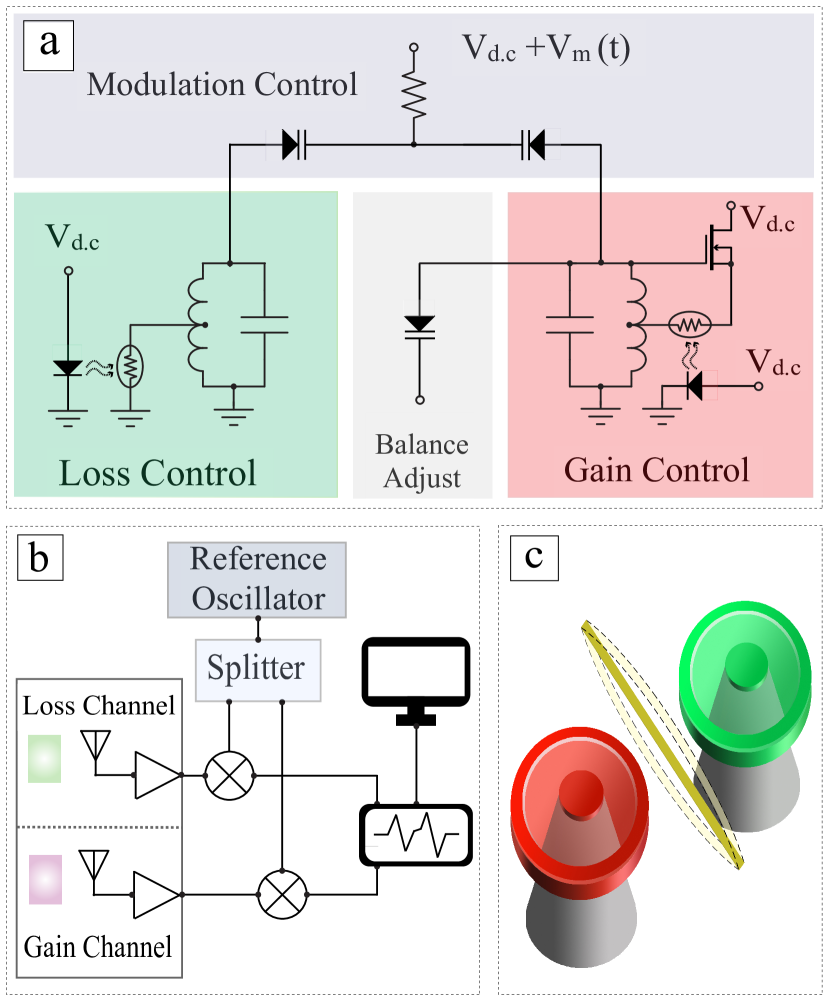
Figure 1: (Color Online) (a) Experimental ${\cal PT}$ circuit with tuning and modulation control; (b) Signal control and analysis system; (c) An analogous mechanically modulated coupling (via a vibrating candilever) between two optical resonators, one with gain (red) and the other with loss (green).

Here we provide such an experimental platform where periodically driven ${\cal PT}-$symmetric systems can be investigated. Our set-up (see Figs. 1a,b) consists of two coupled LC resonators with balanced gain and loss. The capacitance that couples the two resonators is parametrically driven with a network of varactor diodes. We find that this driven ${\cal PT}$ system supports a sequence of spontaneous ${\cal PT}$-symmetry broken domains bounded by exceptional point degeneracies. The latter are analyzed and understood theoretically using an equivalent Floquet frequency lattice with local ${\cal PT}$- symmetry. The position and size of these instability islands can be controlled through the amplitude and frequency of the driving and can be achieved, in principle, for arbitrary values of the gain/loss parameter.

Experimental set-up– A natural frequency of $\omega_{0}/2\pi=235$ MHz was chosen as the highest frequency convenient for a simple implementation of electronic gain and loss. The $L=32$ nH inductors of Fig. 1a are two-turns of 1.5 mm diameter Cu wire with their hot ends supported by their corresponding parallel $C=15$ pF on opposite sides of a grounded partition separating gain and loss compartments. Gain and loss (corresponding to effective parallel resistances $\mp R$) are directly implemented via Perkin-Elmer V90N3 photocells connecting the center turn of each inductor either directly to ground (loss side) or to a BF998 MOSFET following the $LC$ node (gain side). Thus as both photocells experience the same voltage drop, the loss side photocell extracts its current from the tap point while the gain side photocell injects its current into the tap point. The photocells are coupled to computer driven LEDs through 1 cm light-pipes for RF isolation. As the gain of the MOSFET is changed, its capacitance shifts slightly unbalancing the resonators. A BB135 varactor is used to compensate for these changes.

The capacitance coupling network, implemented by similar varactors, is optimized for application of a modulation frequency in the vicinity of $4.6$ MHz modulation frequency while simultaneously providing the DC bias necessary for controlling the inter-resonator coupling $C_{c}$.

Fig. 1b shows the remainder of the signal acquisition set-up. The excitation in each resonator is sensed by a small pickup loop attached to the input of a Minicircuits ZPL-1000 low noise amplifier. The gain and loss pick-up channels are then heterodyned to $\approx 30$ MHz before being captured by a Tektronix DPO2014 oscilloscope.

The experimental unmodulated $\cal{PT}$ diagram, shown with the color-map in Fig. 2a, is matched to the theoretical results in order to calibrate both the resonator frequency balance and the gain/loss balance. The coupling is then modulated, directly comparing each calibrated point with and without the modulation. Signal transients are measured by pulsing the MOSFET drain voltage at approximately $1kHz$ and capturing the resonator responses on both the gain and loss sides. The captured signals can be frequency-analyzed to obtain the modulated (or unmodulated) spectrum, see Fig. 2. Time transients can also be directly analyzed to reveal the time-domain dynamics, see Fig. 3. Close attention has to be paid to avoid saturation of any of the components in the signal pick-up chain.

Theoretical considerations– Using Kirchoff’s laws, the dynamics for the voltages $V_{1}\left(V_{2}\right)$ of the gain (loss) side of the periodically driven dimer is:

$$\frac{d^{2}}{d\tau^{2}}V+A\frac{d}{d\tau}V+BV=0;\quad V\equiv(V_{1},V_{2})^{T},$$ (1)

where $\tau=\omega_{0}t$ is the rescaled time, $\omega_{0}=\frac{1}{\sqrt{LC}}$ and

$$A = \frac{1}{1+2c}\begin{bmatrix}-\gamma\left(1+c\right)+2\stackrel{{\scriptstyle\centerdot}}{{c}}&\gamma c-2\stackrel{{\scriptstyle\centerdot}}{{c}}\\ -\gamma c-2\stackrel{{\scriptstyle\centerdot}}{{c}}&\gamma\left(1+c\right)+2\stackrel{{\scriptstyle\centerdot}}{{c}}\end{bmatrix}$$

$$B = \frac{1}{1+2c}\begin{bmatrix}1+c+\stackrel{{\scriptstyle\centerdot\centerdot}}{{c}}&c-\stackrel{{\scriptstyle\centerdot\centerdot}}{{c}}\\ c-\stackrel{{\scriptstyle\centerdot\centerdot}}{{c}}&1+c+\stackrel{{\scriptstyle\centerdot\centerdot}}{{c}}\end{bmatrix}$$ (2)

Above $\gamma=R^{-1}\sqrt{L/C}$ is the rescaled gain/loss parameter, and $\stackrel{{\scriptstyle\centerdot}}{{c}}$ ($\stackrel{{\scriptstyle\centerdot\centerdot}}{{c}}$) denotes the first (second) derivative of the scaled capacitive coupling $c\equiv\frac{C_{c}}{C}=c_{0}+\varepsilon\cos\left(\omega_{m}\tau\right)$ with respect to the scaled time $\tau$. Equation (1) is invariant under joint parity ${\cal P}$ and time ${\cal T}$ operations, where ${\cal T}$ performs the operation $\tau\rightarrow-\tau$ and ${\cal P}$ is the Pauli matrix $\sigma_{x}$.

The eigenfrequencies $\omega_{\alpha}\>(\alpha=1,2)$ of system Eq. (1) in the absence of driving are given as

$$\omega_{\alpha}= \frac{1}{2\sqrt{1+2c_{0}}}\left(\sqrt{\gamma_{c}^{2}-\gamma^{2}}+\left(-1\right)^{\alpha}\sqrt{\gamma_{PT}^{2}-\gamma^{2}}\right)$$ (3)

where the spontaneous ${\cal PT}$- symmetry breaking point and the upper critical point can be identified as $\gamma_{{\cal PT}}=\sqrt{1+2c_{0}}-1$ and $\gamma_{c}=\sqrt{1+2c_{0}}+1$ respectively, and they are both determined by the strength of the (capacitance) coupling between the two elements of the dimer. A parametric evolution of these modes, versus the gain/loss parameter $\gamma$, is shown in Fig. 2a where the open circles are Eq. (3) and the color map shows the experimental results. We find that the spectrum is divided in two compact domains of exact ($\gamma<\gamma_{\cal PT}$) and broken ($\gamma>\gamma_{\cal PT}$) ${\cal PT}$-symmetric domains.

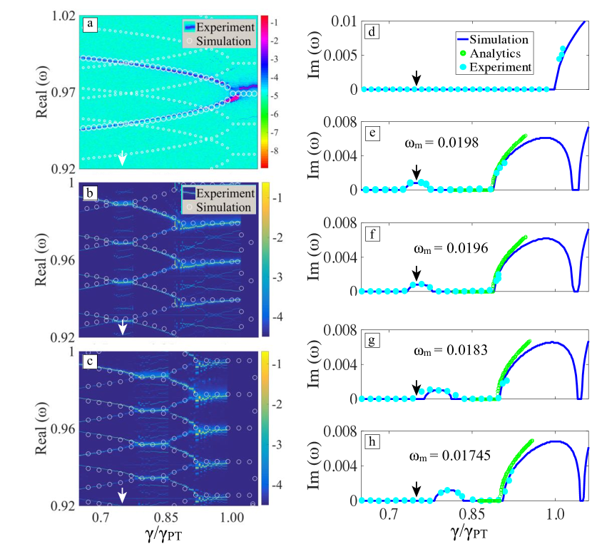
Figure 2: (Color Online) Density plots for ${\cal R}e\left(\omega\right)$ of the RLC dimer of Fig. 1a,b : (a) Undriven dimer $\epsilon=0$. The white cycles represent the ladder $\omega_{1,2}+n\omega_{m}$ associated with the eigenfrequencies of $H_{F,0}$ for $\omega_{m}=0.0198$. The crossing points “evolve” to flat regions when the system is driven with (b) $\omega_{m}=0.0198$. (c) For different driving frequency $\omega_{m}=0.01745$ the flat regions shift to different $\gamma$-domains. The white circles in (b,c) represent the results of the simulations Fnote . Experimental measurements (aqua circles), numerics (blue line) and perturbation theory Eq. (11) (green circles) of ${\cal I}m\left(\omega\right)$ for (d) an undriven dimer and driven dimers with (e) $\omega_{m}=0.0198$ and (f) $\omega_{m}=0.0196$ (g) $\omega_{m}=0.0183$ and (h) $\omega_{m}=0.01745$. In all cases the DC capacitance is $c_{0}=0.0671$ while the amplitude of the driving capacitance is $\epsilon=0.01$.

In order to investigate the effects of driving we now turn to the Floquet picture. A simple way to do this is by employing a Liouvillian formulation of Eq. (1). The latter takes the form

$$\frac{d\psi}{d\tau}= \mathcal{L}\psi,\quad\>\mathcal{L}=\begin{bmatrix}0&I_{2}\\ -B&-A\end{bmatrix},\,\,\,\,\psi=\left(\begin{matrix}V\\ \stackrel{{\scriptstyle\centerdot}}{{V}}\end{matrix}\right)$$ (4)

and allows us to make equivalences with the time-dependent Schrödinger equation by identifying a non-Hermitian effective Hamiltonian $H_{eff}=\imath{\mathcal{L}}$.

The general form of the solution of Eq. (4) is given by Floquet’s theorem which in matrix notation reads $F\left(\tau\right)=\Phi\left(\tau\right)e^{-\imath Q\tau}$ with $\Phi\left(\tau+\frac{2\pi}{\omega_{m}}\right)=\Phi\left(\tau\right)$, $Q$ a Jordan matrix and $F(\tau)$ a $4\times 4$ matrix consisting of four independent solutions of Eq. (4). The eigenvalues of $Q$ are the characteristic exponents (quasi-energies) which determine the stability properties of the system: namely the system is stable (exact ${\cal PT}$ phase) if all the quasi-energies are real and it is unstable (broken ${\cal PT}$ phase) otherwise. We can evaluate the quasi-energies by constructing the evolution operator $U\left(\tau,0\right)=F(\tau)F^{-1}(0)$ via numerical integration of Eq. (6) (or of Eq. (1)). Then the quasi-energies are the eigenvalues of $\frac{1}{-\imath 2\pi/\omega_{m}}\ln U\left(\tau=2\pi/\omega_{m},0\right)$.

In Figs. 2a-h we report our numerical findings together with the experimentally measured values of the quasi-energies versus the gain/loss parameters. Figs. 2a,d show the unmodulated situation. Fig. 2b,e show the behavior at modulation frequency $\omega_{m}=0.0198$ and modulation amplitude $\epsilon=0.01$. Finally, Figs 2c,e-h show the evolution of the spectrum with a small change in modulation frequency $\omega_{m}$ for fixed $\epsilon$. Only one of the real part color-maps, $\omega_{m}=0.01745$, is shown.

We find several new features in the spectrum of the driven ${\cal PT}$-symmetric systems. The first difference with respect to the undriven case is the existence of a cascade of domains for which the system is in the broken ${\cal PT}$-phase. These domains are identified by the flat regions, seen in Figs. 2b,c where the real parts of eigenfrequencies have merged, or by the emerging non-zero imaginary parts shown in Figs. 2e-h. The size and position of these unstable “bubbles” are directly controlled by the values of the driving amplitude $\epsilon$, compare Figs. 2a,d with Figs. 2b,e or by the driving frequency $\omega_{m}$, compare Figs. 2b,e with Figs. 2c,h. The bubbles are separated by $\gamma$-domains where the system is in the exact (stable) ${\cal PT}$-phase. The transition between stable and unstable domains occurs via a typical EP degeneracy (notice the square -root singularities in Figs. 2d-h).

A theoretical understanding of the spectral metamorphosis from a single compact exact/broken phase to multiple domains of broken and preserved ${\cal PT}$-symmetry, as $\epsilon$ increases from zero, is achieved by utilizing the notion of Floquet Hamiltonian $H_{F}$. To this end, we first introduce a time-dependent similarity transformation ${\cal R}$, which brings the effective Hamiltonian matrix that dictates the evolution in the Schrödinger-like equation to a symmetric form. We shall see below that the symmetric form is inherited in the Floquet Hamiltonian (up to the first order perturbation in $\epsilon$ and $\omega_{m}\sim O(\varepsilon)$). Consequently the bi-orthogonal Floquet eigenmodes of the unperturbed Floquet matrix are transpose of each other – a property that greatly simplifies the analytical process for the evaluation via first-order theory of the Floquet eigenmodes. This transformation takes the form SLZEK11 :

$${\cal R}\left(\tau\right)= \begin{bmatrix}1&1&\imath\sqrt{\beta}&-\imath\sqrt{\beta}\\ \sqrt{1+2\stackrel{{\scriptstyle\centerdot\centerdot}}{{c}}}&-\sqrt{1+2\stackrel{{\scriptstyle\centerdot\centerdot}}{{c}}}&\imath&\imath\\ -\sqrt{1+2\stackrel{{\scriptstyle\centerdot\centerdot}}{{c}}}&\sqrt{1+2\stackrel{{\scriptstyle\centerdot\centerdot}}{{c}}}&\imath&\imath\\ 1&1&-\imath\sqrt{\beta}&\imath\sqrt{\beta}\end{bmatrix}$$ (5)

and allows us to bring Eq. (4) to the following Schrödinger-like form

$$\imath\frac{d}{d\tau}\tilde{\psi}= {\tilde{H}}\tilde{\psi};\quad{\tilde{H}}\equiv{\cal R}H_{eff}{\cal R}^{-1}-\imath{\cal R}\frac{d}{d\tau}{\cal R}^{-1}$$ (6)

which dictates the evolution of the transformed state $\tilde{\psi}={\cal R}\psi$. The matrix ${\tilde{H}}$ satisfies the relation ${\tilde{H}}={\tilde{H}}^{T}$, i.e. it is transposition symmetric, and has the form

$${\tilde{H}}= \begin{bmatrix}-\frac{3}{2}\frac{\imath\stackrel{{\scriptstyle\centerdot}}{{c}}}{\beta}&c_{+}+\frac{\imath\gamma}{2\sqrt{\beta}}&c_{-}+\frac{\imath\gamma}{2\sqrt{\beta}}&\frac{3}{2}\frac{\imath\stackrel{{\scriptstyle\centerdot}}{{c}}}{\beta}\\ c_{+}+\frac{\imath\gamma}{2\sqrt{\beta}}&\frac{\imath c^{(3)}}{2(1+2\stackrel{{\scriptstyle\centerdot\centerdot}}{{c}})}&-\frac{\imath c^{(3)}}{2(1+2\stackrel{{\scriptstyle\centerdot\centerdot}}{{c}})}&c_{-}-\frac{\imath\gamma}{2\sqrt{\beta}}\\ c_{-}+\frac{\imath\gamma}{2\sqrt{\beta}}&-\frac{\imath c^{(3)}}{2(1+2\stackrel{{\scriptstyle\centerdot\centerdot}}{{c}})}&\frac{\imath c^{(3)}}{2(1+2\stackrel{{\scriptstyle\centerdot\centerdot}}{{c}})}&c_{+}-\frac{\imath\gamma}{2\sqrt{\beta}}\\ \frac{3}{2}\frac{\imath\stackrel{{\scriptstyle\centerdot}}{{c}}}{\beta}&c_{-}-\frac{\imath\gamma}{2\sqrt{\beta}}&c_{+}-\frac{\imath\gamma}{2\sqrt{\beta}}&-\frac{3}{2}\frac{\imath\stackrel{{\scriptstyle\centerdot}}{{c}}}{\beta}\end{bmatrix},$$ (7)

where $\beta=1+2c,c_{\pm}=\frac{1}{2}\pm\frac{1}{2}\frac{\sqrt{1+2\stackrel{{\scriptstyle\centerdot\centerdot}}{{c}}}}{\sqrt{\beta}}$ and $c^{(3)}$ denotes the third derivative of the capacitive coupling with respect to the scaled time $\tau$. We can easily show that $\tilde{\cal P}{\cal T}{\tilde{H}}\tilde{\cal P}{\cal T}={\tilde{H}}$ where ${\tilde{\cal P}}=\begin{bmatrix}0&\sigma_{x}\\ \sigma_{x}&0\end{bmatrix}$ and the time-reversal operator is defined as ${\cal T}:\tau\rightarrow-\tau,\imath\rightarrow-\imath$.

We are now ready to utilize the notion of Floquet Hamiltonian $H_{F}$ whose components are given by

$$\left\langle\alpha,n\right|H_{F}\left|\beta,l\right\rangle= {\tilde{H}}_{\alpha\beta}^{\left(n-l\right)}+n\omega_{m}\delta_{\alpha\beta}\delta_{nl},$$ (8)

where the subscripts $\alpha,\beta=1,2,3,4$ label the components of ${\tilde{H}}$, see Eq. (7), $n,l$ are any integers and ${\tilde{H}}_{\alpha\beta}^{\left(n\right)}=\frac{1}{2\pi/\omega_{m}}\int_{0}^{2\pi/\omega_{m}}{\tilde{H}}_{\alpha\beta}\left(\tau\right)e^{-\imath n\omega_{m}\tau}d\tau$. In this picture the quasi-energies are the eigenvalues of the Floquet Hamiltonian $H_{F}$. Note, that Eq. (8) defines a lattice model with complex connectivity given by the off-diagonal elements of $H_{F}$ and an on-site gradient potential $n\omega_{m}$. These type of lattices (though in real space) have been recently investigated in the frame of waveguide photonics and have been shown to generate Bloch-Zener type of dynamics BLEK15 . Thus our set-up can be used as a user-friendly experimental framework for the investigation of dynamics in such complicated lattices where the lattice complexity enters via a designed driving scheme.

Within the first order approximation to the strength of the driving amplitude $\varepsilon$ and the modulation frequency $\omega_{m}\sim O(\varepsilon)$, the Floquet Hamiltonian is symmetric and takes the block-tridiagonal form $H_{F}=H_{F,0}+\varepsilon H_{F,1}+O\left(\varepsilon^{2}\right)$ where $\left\langle n\right|H_{F,0}\left|n\right\rangle={\tilde{H}}^{\left(0\right)}\left|{}_{\varepsilon=0}\right.+n\omega_{m}I_{4}$ consists of the diagonal blocks of $H_{F}$ while $\left\langle n+1\right|H_{F,1}\left|n\right\rangle=\left\langle n\right|H_{F,1}\left|n+1\right\rangle=X$ consist of off-diagonal blocks of $H_{F}$. The $4\times 4$ matrix $X$ has the form note1

$$X=\frac{\imath}{4\left(1+2c_{0}\right)^{3/2}} \begin{bmatrix}0&\imath-\gamma&-\imath-\gamma&0\\ \imath-\gamma&0&0&-\imath+\gamma\\ -\imath-\gamma&0&0&\imath+\gamma\\ 0&-\imath+\gamma&\imath+\gamma&0\end{bmatrix}.$$ (9)

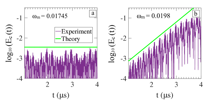
Figure 3: (Color Online) Temporal evolution of normalized total capacitance energy $E_{c}(t)=\left(V_{1}^{2}(t)+V_{2}^{2}(t)\right)$ (in units of Volt²). The green lines indicate the theoretical predictions (from simulations) for the slope of the envelope for driving frequencies (a) $\omega_{m}=0.01745$ and (b) $\omega_{m}=0.0198$. In both cases the value of $\gamma$ is the same (see black arrows in Fig. 2e,h).

Next we proceed with the analytical evaluation of the quasi-energies. First, we neglect the off-diagonal block matrices $H_{F,1}$ and diagonalize $H_{F,0}$. To this end, we construct a similarity transformation $P_{0}^{-1}H^{\left(0\right)}\left|{}_{\varepsilon=0}\right.P_{0}=diag\left\{\omega_{2},\omega_{1},-\omega_{1},-\omega_{2}\right\}$. Correspondingly the eigenvalues of $H_{F,0}$ are simply $\left\{\omega_{2}+n\omega_{m},\omega_{1}+n\omega_{m},-\omega_{1}+n\omega_{m},-\omega_{2}+n\omega_{m}\right\}$ where $n$ is an integer i.e. the spectrum resembles a ladder of step $\omega_{m}$ and basic unit associated with the eigenfrequencies of the undriven dimer Eq. (3). The resulting ladder spectrum (white circles) is shown in Fig. 2a versus the gain/loss parameter $\gamma$. Level crossing occurs at some specific values of $\gamma^{\left(j\right)}$, i.e., $\omega_{2}\left|{}_{\gamma^{\left(j\right)}}\right.=\omega_{1}\left|{}_{\gamma^{\left(j\right)}}\right.+j\omega_{m}$. When the driving amplitude $\varepsilon$ is turned on, the crossing points evolve to broken ${\cal PT}$-symmetry domains with respect to gain/loss parameter $\gamma$ (see Figs. 2b,c). Specifically the real part of the eigenfrequencies become degenerate for a range of $\gamma$-values around $\gamma^{(j)}$, Fig. 2b, while an instability bubble emerges for the imaginary part – see Fig. 2e where numerical (blue solid lines) and experimental data (filled aqua circles) agree nicely with one another. The transition points from stable to unstable domains have all the characteristic features of an EP i.e. a square root singularity of the spectrum and degeneracy of the eigenmodes (not shown).

To understand this phenomenon, we now consider the effect of the additional off-diagonal term $\varepsilon H_{F,1}$. For simplicity, we focus on the unstable region around the crossing point at $\gamma^{\left(1\right)}$. Application of degenerate perturbation theory to the nearly degenerate levels $\omega_{2}$ and $\omega_{1}+\omega_{m}$ gives

$$\omega= \frac{\left(\omega_{2}+\omega_{1}+\omega_{m}\right)\pm\sqrt{\left(\omega_{2}-\omega_{1}-\omega_{m}\right)^{2}+4\varepsilon^{2}\tilde{X}_{12}\tilde{X}_{21}}}{2},$$ (10)

where $\tilde{X}=P_{0}^{-1}XP_{0}$ and the subscripts indicate the corresponding matrix components. Explicitly, around the EP, $\omega$ can be written as

$$\mathrm{Re}\left(\omega\right)\approx\omega_{2}\left|{}_{\gamma^{\left(1\right)}}\right.;\,\,\mathrm{Im}\left(\omega\right)= \pm C_{m}\sqrt{\gamma-\gamma_{0}},\,\,\gamma>\gamma_{0}$$ (11)

which has the characteristic square-root singularity of EP degeneracies. The constant $C_{m}$ takes the form

$$C_{m}= \frac{1}{2}\sqrt{\frac{1}{\gamma_{PT}^{2}-\gamma_{0}^{2}}\frac{\varepsilon\gamma_{0}}{1+2c_{0}}\left[\left(\frac{2}{\sqrt{1+2c_{0}}}-\frac{\omega_{m}}{\sqrt{\gamma_{PT}^{2}-\gamma_{0}^{2}}}\right)\gamma_{0}+\frac{\varepsilon}{2\left(1+2c_{0}\right)}\right]}$$ (12)

and $\gamma_{0}$ is the solution of the equation $\left(\omega_{2}-\omega_{1}-\omega_{m}\right)^{2}+4\varepsilon^{2}\tilde{X}_{12}(\gamma)\tilde{X}_{21}(\gamma)=0$ (see Eq. (9)) note2 . From Eq. (11) we clearly see that both $\omega_{m},\epsilon$ are responsible for a renormalization of the coupling between the two levels (compare with Eq. (3)).

Predictions (11) are in agreement with the numerical and experimental data (see green line in Fig. 2e-h). Higher orders of EPs $\gamma^{(j)}$ can be analyzed in a similar manner. In this case, however, the small size of the instability bubbles require to take into consideration higher order perturbation theory corrections in order to describe the quasi-energies $\omega$. We have, nevertheless tested the applicability of this scheme via numerical evaluation of the higher order corrections.

The management of the exact and broken ${\cal PT}$ symmetry phase, either via the driving amplitude $\epsilon$ or via the frequency $\omega_{m}$, has also direct implications to the dynamics of the system. In Fig.3 we report the total capacitance energy of the dimer for the same $\gamma=0.0483$ and $\epsilon=0.01$ values but different driving frequencies $\omega_{m}=0.01745$ (left) and $\omega_{m}=0.0198$ (right). In the latter case the energy grows exponentially with a rate given by the imaginary part of the eigenfrequencies (see Fig. 2e) while in the former we have an oscillatory (stable) dynamics (see Fig. 2h).

Conclusions– We have experimentally demonstrated that ${\cal PT}$-symmetric systems containing periodically driven components are capable of controlling the presence, strengths, and positions of multiple exact-phase domains, bounded by corresponding exceptional points. The generic behavior is well described by a perturbative analysis of the Floquet Hamiltonian, and opens up new directions of exceptional point management in a variety of electronic, mechanical or optimechanical applications, similar to the example shown in Fig. 1c.

Acknowledgments – This research was partially supported by an AFOSR grant No. FA 9550-10-1-0433, and by NSF grants ECCS-1128571 and DMR-1306984.

References

- (1) C. M. Bender, S. Boettcher, Phys. Rev. Lett. 80, 5243 (1998); C. M. Bender, Rep. Prog. Phys. 70, 947 (2007).
- (2) K. G. Makris et al., Phys. Rev. Lett. 100, 103904 (2008).
- (3) S. Longhi, Phys. Rev. Lett. 103, 123601 (2009); S. Longhi, Phys. Rev. Lett. 105, 013903 (2010).
- (4) C. E. Rüter et al., Nat. Phys. 6, 192 (2010); A. Guo, et al., Phys. Rev. Lett. 103, 093902 (2009).
- (5) M. C. Zheng et. al, Phys. Rev. A 82, 010103 (2010).
- (6) H. Schomerus, Phys. Rev. Lett. 104, 233601 (2010).
- (7) A. A. Sukhorukov, Z. Xu, Y. S. Kivshar, Phys. Rev. A 82, 043818 (2010).
- (8) S. Longhi, Phys. Rev. A 82, 031801 (2010); Y. D. Chong et al., Phys. Rev. Lett. 106, 093902 (2011).
- (9) L. Feng et al., Science 333, 729 (2011).
- (10) A. Regensburger, C. Bersch, M.A. Miri, G. Onishchukov, D. N. Christodoulides, U. Peschel, Nature 488, 167 (2012).
- (11) H. Ramezani, D. N. Christodoulides, V. Kovanis, I. Vitebskiy, T. Kottos, Phys. Rev. Lett. 109, 033902 (2012); H. Ramezani, T. Kottos, V. Kovanis, D. N. Christodoulides, Phys. Rev. A 85, 013818 (2012).
- (12) L. Chang et al., Nat. Phot. 8, 524 (2014).
- (13) B. Peng et al., Nat. Phys. 10, 394 (2014).
- (14) H. Hodaei et al., Science 346, 975 (2014); L. Feng et al., Science 346, 972 (2014).
- (15) N. Lazarides and G. P. Tsironis, Phys. Rev. Lett. 110, 053901 (2013); D. Wang, A. B. Aceves, Phys. Rev. A 88, 043831 (2013).
- (16) H. Ramezani et al., Optics Express 20, 26200 (2012).
- (17) Z-P. Liu, J. Zhang, S K. Özdemir, B. Peng, H. Jing, X-Y. Lü, C-W. Li, L. Yang, F. Nori, Y-x Liu, Phys. Rev. Lett. 117, 110802 (2016).
- (18) B. Peng, S. K. Ozdemir, S. Rotter, H. Yilmaz, M. Liertzer, F. Monifi, C. M. Bender, F. Nori, L. Yang, Science, 346, 328 (2014)
- (19) H. Cartarius, G. Wunner, Phys. Rev. A 86, 013612 (2012); M. Kreibich, J. Main, H. Cartarius, G. Wunner, Phys. Rev. A 87, 051601(R) (2013); M. Kreibich, J. Main, H. Cartarius, G. Wunner, Phys. Rev. A 90, 033630 (2014); W. D. Heiss, H. Cartarius, G. Wunner, J. Main, J. Phys. A: Math. Theor. 46, 275307 (2013).
- (20) E-M Graefe, J. Phys. A: Math. Theor. 45, 444015 (2012); M. Hiller, T. Kottos, A. Ossipov, Phys. Rev. A 73, 063625 (2006)
- (21) J. M. Lee, T. Kottos, B. Shapiro, Phys. Rev. B 91, 094416 (2015)
- (22) A. Galda, V. M. Vinokur, Phys. Rev. B 94, 020408(R) (2016)
- (23) X. Zhu, H. Ramezani, C. Shi, J. Zhu, X. Zhang, Phys. Rev. X 4, 031042 (2014).
- (24) R. Fleury, D. Sounas, A. Alu, Nat. Commun. 6, 5905 (2014).
- (25) C. Shi, M. Dubois, Y. Chen, L. Cheng, H. Ramezani, Y. Wang, X. Zhang, Nat. Commun. 7, 11110 (2016)
- (26) J. Schindler et al., J. Phys. A -Math and Theor. 45, 444029 (2012); H. Ramezani et al., Phys. Rev. A 85, 062122 (2012); Z. Lin et al., Phys. Rev. A 85, 050101(R) (2012); N. Bender, S. Factor, J. D. Bodyfelt, H. Ramezani, D. N. Christodoulides, F. M. Ellis, T. Kottos, Phys. Rev. Lett. 110, 234101 (2013)
- (27) J. Cuevas, P. G. Kevrekidis, A. Saxena, A. Khare, Phys. Rev. A 88, 032108 (2013);F. Bagarello Phys. Rev. A 88, 032120 (2013).
- (28) I. V. Barashenkov, M. Gianfreda, J. Phys. A: Math. Theor. 47, 282001 (2014)
- (29) C. T. West, T. Kottos, T. Prosen, Phys. Rev. Lett. 104, 054102 (2010)
- (30) N. Moiseyev, Phys. Rev. A 83, 052125 (2011)
- (31) R. El-Ganainy, K. G. Makris, D. N. Christodoulides, Phys. Rev. A 86, 033813 (2012).
- (32) G. Della Valle, S. Longhi, Phys. Rev A 87, 022119 (2013)
- (33) X. Luo, J. Huang, H. Zhong, X. Qin, Q. Xie, Y. S. Kivshar, C. Lee, Phys. Rev. Lett. 110, 243902 (2013); X-B Luo, R-X Liu, M-H Liu, X-G Yu, D-L Wu, Q-L Hu, Chin. Phys. Lett. 31, 024202 (2014).
- (34) X. Lian, H. Zhong, Q. Xie, X. Zhou, Y. Wu, W. Liao, Eur. Phys. J. D 68, 189 (2014)
- (35) D. Psiachos, N. Lazarides, G. P. Tsironis, Appl. Phys. A - Mat. Sc. Proc. 117, 663 (2014); G. P. Tsironis, G. P.; N. Lazarides, Appl. Phys. A- Mat. Sc. Proc. 115, 449 (2014).
- (36) V. V. Konotop, D. A. Zezyulin, Optics Lett. 39, 1223 (2014)
- (37) J. D’Ambroise, B. A. Malomed, P. G. Kevrekidis, Chaos 24, 023136 (2014).
- (38) Y. N. Joglekar, R. Marathe, P. Durganandini, R. Pathak, Phys. Rev. A 90, 040101(R) (2014); T. E. Lee, Y. N. Joglekar, Phys. Rev. A 92, 042103 (2015).
- (39) Y. Wu, B. Zhu, S-F Hu, Z. Zhou, H Zhong, Front. Phys. 12, 121102 (2017)
- (40) M. O. Scully, M. S. Zubairy, Quantum Optics (Cambridge University Press, Cambridge, 1997).
- (41) S. H. autler, C. H. Townes, Phys. Rep. 100, 703 (1955).
- (42) D. H. Dunlap, V. M. Kenkre, Phys. Rev. B 34, 3625 (1986).
- (43) B. V. Chirikov, F. M. Izrailev, D. L. Shepelyansky, Sov. Sci. Rev. Sect. C 2, 209 (1981).
- (44) F. Grossmann, T. Dittrich, P. Jung, P. Hänggi, Phys. Rev. Lett. 67, 516 (1991).
- (45) G. Della Valle, M. Ornigotti, E. Cianci, V. Foglietti, P. Laporta, S. Longhi, Phys. Rev. Lett. 98, 263601 (2007).
- (46) M. Grifoni, P. Hänggi, Phys. Rep. 304, 229 (1998).
- (47) N. H. Lindner, G. Rafael, V. Galitski, Nat. Phys. 7, 490 (2011)
- (48) Y. H. Wang, H. Steinberg, P. Jarillo-Herrero, N. Gedik, Science 342, 453 (2013)
- (49) N. Bender, H. Li, F. M. Ellis, T. Kottos, Phys. Rev. A 92, 041803(R) (2015).
- (50) It turns out that for our specific experimental parameters . Nevertheless in our calculation scheme we include the terms in the part since they are analytically easy to deal with.
- (51) In the specific case of and after taking into consideration our experimental case and we can explicitly solve and have that .
- (52) Note that the real parts in Figs. 2b,c include a mode translated from the negative frequency domain of the Floquet latice that is not shown due to its practical insignificance and enhanced sensitivity to drive frequency.