IGR J17062$-$6143 is an Accreting Millisecond X-ray Pulsar

Abstract

We present the discovery of 163.65 Hz X-ray pulsations from IGR J17062$-$6143 in the only observation obtained from the source with the Rossi X-ray Timing Explorer. This detection makes IGR J17062$-$6143 the lowest-frequency accreting millisecond X-ray pulsar presently known. The pulsations are detected in the 2 - 12 keV band with an overall significance of $4.3\sigma$, and an observed pulsed amplitude of $5.54\pm 0.67\%$ (in this band). Both dynamic power spectral and coherent phase timing analysis indicate that the pulsation frequency is decreasing during the $\approx 1.2$ ks observation in a manner consistent with orbital motion of the neutron star. Because the observation interval is short, we cannot precisely measure the orbital period; however, periods shorter than 17 minutes are excluded at $90\%$ confidence. For the range of acceptable circular orbits the inferred binary mass function substantially overlaps the observed range for the AMXP population as a whole.

1. Introduction

There is now compelling evidence that millisecond pulsars are “recycled,” meaning that they have acquired their rapid spins via accretion during their binary evolution. A compelling demonstration of the recycling scenario was provided by the discovery in 1998 of the first accreting millisecond X-ray pulsar (AMXP), SAX J1808.4$-$3658 (hereafter J1808). This system comprises a 401 Hz pulsar in a 2.01 hr binary (Wijnands & van der Klis 1998; Chakrabarty & Morgan 1998). It remains the “prototype,” and best-studied member of the class, and exhibits all of the defining properties of AMXPs: short orbital periods (less than a few hours, and often less than an hour), low time-averaged accretion rates, and very low mass donors ($\leqslant 0.2M_{\odot}$). It has now been eighteen years since the discovery of J1808, and still only 16 such sources have been identified (see Patruno & Watts 2012 for a review), the most recent being Monitor of All-sky X-ray Image (MAXI) J0911$-$655 (Sanna et al. 2016).

In this Letter, we present evidence based on an observation performed in 2008 May with the Rossi X-ray Timing Explorer (RXTE; Bradt et al. 1993) that IGR J17062$-$6143 is an AMXP with a pulsation frequency of 163.65 Hz. The source (also classified as SWIFT J1706.6$-$6146) is an accreting neutron star binary, first observed during an outburst in 2006 (Churazov et al. 2007; Ricci et al. 2008; Remillard & Levine 2008). The outburst has persisted at a low flux level since then, and the source has also produced several bright X-ray bursts, confirming that the accretor is a neutron star. The first of these was observed by Swift in 2012 following an on-board trigger from the Swift/BAT (Degenaar et al. 2013), and more recently, a long-duration burst, possibly powered by a thick helium layer (Keek et al. 2016), was detected by the MAXI all-sky monitor (Negoro et al. 2015). Both events exhibited signs that the bursts had a strong impact on the accretion environment around the neutron star. This included variability in the X-ray light curve as well as reflection features in the spectrum. Reflection signatures were also detected by NuSTAR in observations of the persistent flux (Degenaar et al. 2017; Keek et al. 2016). They indicate that the accretion disk is truncated at $\sim 10^{2}\,R_{\mathrm{g}}$, where $R_{\mathrm{g}}=GM/c^{2}$ is the gravitational radius. A relatively strong magnetic field could potentially provide the support for the truncated inner disk.

We first present the results of our pulsation search of IGR J17062$-$6143 and describe the discovery of pulsations (Section 2). We show that the pulse frequency varies with time in a manner consistent with orbital motion of the neutron star. We further use coherent timing methods to place a lower limit on the orbital period of about 17 minutes. The energy spectrum is analyzed to quantify the mass accretion rate at the time of the observation. Next, we estimate the magnetic field strength, and we discuss whether it supports the picture of the accretion geometry that was inferred by the reflection spectra (Section 3).

2. Pulsation Search with RXTE

Perhaps surprisingly, RXTE observed IGR J17062$-$6143 only once, in 2008 May for a total of $\approx 1200$ s (obsid: 93437-01-01-00). We used this single observation to search for pulsations. In addition to the standard Proportional Counter Array (PCA) data modes, high time resolution data were acquired in the E_125us_64M_0_1s event mode, which provides a time resolution of 1/8192 s in 64 energy bins. For this observation only two of the five Proportional Counter Units (PCUs) comprising the full PCA array were active (PCUs 0 and 2, in the 0-4 numbering scheme). We used the standard RXTE data analysis tools to extract light curves, spectra, and an estimate of the background spectrum during the observation. We used the tool faxbary to compute barycentric arrival times for all events. For this purpose we used the source position, $R.A.=256.5677$, decl. $=-61.7113$, from Ricci et al. (2008). We used the barycentered events to construct light curves with 1/8192 second resolution (for a Nyquist frequency of 4096 Hz) and the observation had a useful exposure of 1168 s.

Since the background provides a significant fraction of the total count rate, we carried out a pulsation search in two energy bands. The first used all counts across the entire PCA response. For the second we found the energy channel below which the source count rate is greater than the background counting rate and only used events with energy less than or equal to this value. We found that channel 16 (of the 64 bins of the data mode) satisfied this condition, so we produced a light curve using only events in channels 16 and lower. For this data mode and observation epoch, that channel corresponds to photons with energies less than or equal to $\approx 12$ keV. Figure 1 shows the resulting light curve at 1 s resolution in the $2-12$ keV band, as well as the estimated background (red curve) at 16 s resolution computed from pcabackest.

We computed Leahy-normalized power spectra for each light curve and searched for pulsations in the frequency range from 10 to 2048 Hz. Since orbital motion can induce frequency drifts, we carried out a “hierarchical” search by averaging adjacent Fourier powers in frequency space by a factor, $W$, and also searched the averaged spectra. We used values of $W=1,2,4,8,16$, for a total of 10 power spectra searched. We found a strong pulsation candidate at 163.655 Hz in the power spectrum computed using only the 2 - 12 keV events and averaged by a factor of $W=8$. Figure 2 shows this power spectrum, revealing the strong peak near 163.65 Hz. The putative signal peak has a power value of 11.646.

In such a “hierarchical” search, the rigorous way to assess significances is via Monte Carlo simulations because the distribution of noise powers is different for each averaged power spectrum (van der Klis 1989). First, we note that in the absence of signal power (the null hypothesis) the power values in an averaged power spectrum are distributed such that the probability that a power $P_{j}$ will exceed some value $P$ is given by $Q_{\chi^{2}}(WP,2W)$, where $Q_{\chi^{2}}$ is the integral probability of the $\chi^{2}$ distribution with $2W$ degrees of freedom. As above, $W$ is the averaging factor, and with $W=1$ the familiar $\chi^{2}$ distribution with 2 degrees of freedom is obtained. Thus, the peak power value of 11.646 has a chance occurrence, per trial, given by the probability of obtaining a value of $8\times 11.646=93.17$ from a $\chi^{2}$ distribution with 16 degrees of freedom. This single trial probability is $6.5\times 10^{-13}$. To arrive at our significance estimate, we carried out Monte Carlo simulations that precisely mimic our search procedures. We simulate two light curves with the same mean count rates as our observed light curves. To do this, we generate Poisson realizations using the same time bin size and light curve duration as observed. We then compute averaged power spectra for each simulated light curve using $W=1,2,4,8,16$, and we identify in each spectrum the frequency bins within our $10-2048$ Hz search range. For each of these bins we determine the single trial probability using the appropriate $Q_{\chi^{2}}(WP,2W)$ distribution, and we test whether any bin has a single trial probability less than or equal to the observed value ($6.5\times 10^{-13}$) of the putative signal peak. We repeat the process many times to determine how often a single trial probability this small is achieved in at least one of the light curves. We also determined the number of times that several larger (less significant) single trial probabilities were exceeded, and in this way we determined the $3\sigma$ confidence detection threshold, which is plotted as the horizontal dashed line in Figure 2. From $5\times 10^{5}$ simulations we find a significance of $\approx 1.6\times 10^{-5}$ for the 163.65 Hz pulsation, which is better than a $4\sigma$ detection.

As a consistency check, we used the $W=8$ power spectrum (see Figure 2) in the range from 2048 to 4096 Hz (where no signal power is expected, and we did not search) to explore the distribution of powers and see whether it tracks the expected distribution. We found that the distribution of noise powers in this power spectrum matches well with the expected $Q_{\chi^{2}}(8P,16)$ distribution, giving us additional confidence that our significance estimate is robust.

2.1. Evidence for Orbital Motion

We next computed dynamic power spectra in order to determine if any secular variations in the pulsation frequency, as would be produced by orbital motion of the neutron star, could be discerned. Since the signal strength is relatively modest, and there is only a single RXTE orbit of data, we used a relatively long time interval of 512 s to compute power spectra, and then shifted the center of the interval by 16 s to compute a dynamic spectrum. Figure 3 shows a map of contours of constant Fourier power versus time and frequency from this analysis. The contours are drawn at the time corresponding to the center of each time interval used to compute a power spectrum. Nine contours are drawn at power levels of 20, 22, 24, 26, 28, 30, 32, 36, and 40. Because the segments overlap, each power spectral measurement is not completely independent; nevertheless, the time evolution of the Fourier power is indicative of a decrease in pulsation frequency during the observation, which would not be unexpected for orbital motion of the neutron star. The apparent variation in frequency of $\Delta\nu\approx 0.002$ Hz is likely a lower limit to the full range of any orbitally induced variations. This corresponds to a lower limit on the projected neutron star velocity of $v/c=\Delta\nu/\nu_{0}\approx 1.22\times 10^{-5}$ or $\approx 3.7$ km s^-1, which is consistent with measurements of other AMXPs (see, for example, Markwardt et al. 2002).

To further explore this, we also carried out a coherent timing analysis (see Buccheri et al. 1983; Strohmayer & Markwardt 2002). Since all other AMXPs are adequately described by circular orbits, we used a circular orbit model to describe the time evolution of the average pulsation phase through the observation interval. This model provides a statistically acceptable description of the phase evolution. Further, we also show using this method that a constant frequency model is not consistent with the phase evolution. Figure 4 compares phase timing residuals for these two models. The black square symbols show the phase residuals from the best constant frequency model, which gives an unacceptably high $\chi^{2}$ value of $40.1$ for 5 degrees of freedom. Moreover, the overall trend in these residuals of a concave-up, parabolic shape is strongly indicative of a spin-down of the pulsation frequency, consistent with the dynamic power spectrum (Figure 3). Additionally, in Figure 4, the red diamond symbols show the phase residuals for a circular orbit with a period of 30 minutes. This model gives a good fit to the phase data, with a minimum $\chi^{2}=1.1$ for 2 degrees of freedom. While this orbital model provides an acceptable fit to the phase evolution, because the observation is so short, we cannot precisely determine the orbital period. Indeed, we find that orbits with periods longward of about 17 minutes can all produce acceptable phase residuals; however, we find that the minimum $\chi^{2}$ values rise to unacceptable levels as the orbital period is further reduced, and we find a 90% confidence ($\Delta\chi^{2}=2.71$) lower limit of 17 minutes. We used the best-fitting orbit model with a 30 minute period to phase-fold all the 2 - 12 keV events in order to study the pulse profile and amplitude. The resulting profile is well described by the model, $A+B\sin(\phi-\phi_{0})$. Based on this model, and after subtraction of the background, we find an average source pulsed amplitude of $B/A=9.4\pm 1.1\%$. We also subdivided the observation interval into quarters and measured the amplitude in each, but found no evidence for significant variations in pulsed amplitude.

For the range of acceptable circular orbits we can determine the mass function, $f_{x}=((a\sin i)^{3}\omega_{orb}^{2})/G$, where $a\sin i$ and $\omega_{orb}$ are the projected neutron star orbital radius and frequency, respectively. We find that the mass function increases monotonically from $2\times 10^{-8}$ at a period of 30 minutes to $2.5\times 10^{-6}$ for a period of 100 minutes. This range substantially overlaps with the observed range for other AMXPs (see Patruno & Watts 2012), but, interestingly, if the period is close to 30 minutes, then the mass function would likely be the smallest yet observed and would correspond to a minimum companion mass less than $0.004M_{\odot}$, the smallest to date. Thus, additional observations to pin down the orbital period would be quite important.

2.2. Analysis of the Spectral Energy Distribution

We extracted a single PCA energy spectrum from the full observation interval in the $3-20$  keV energy range using Standard 2 data from the top layer of PCUs $0$ and $2$. The spectrum was analyzed using XSPEC version 12.9.0n (Arnaud 1996). It is well fit by an absorbed power-law model (Figure 5). We employ the Tübingen$-$Boulder model with abundances from Wilms et al. (2000) to model the effects of interstellar absorption. The absorption column is fixed to $N_{\mathrm{H}}=1.58\times 10^{21}\,\mathrm{cm^{-2}}$ (Keek et al. 2016). We find a power-law photon index of $\Gamma=2.21\pm 0.03$ and an unabsorbed $3-20$ keV flux of $F=(1.28\pm 0.02)\times 10^{-10}\mathrm{erg\,s^{-1}\,cm^{-2}}$. $\Gamma$ is only $1.7\,\sigma$ larger than the value measured with Chandra and NuSTAR in 2014 and 2015, respectively (Keek et al. 2016; see also Degenaar et al. 2017), and $F$ is $2.5$ times larger than for the NuSTAR spectrum in the same band. A previous measurement of the source flux during an Eddington-limited, photospheric radius expansion (PRE) episode in a thermonuclear burst suggests a mass accretion rate of $0.6\%$ of the Eddington limit at the time of the PCA observation (Keek et al. 2016). We note that for an assumed Eddington luminosity of $2\times 10^{38}$ erg s^-1, the implied source distance is $\approx 8.8$ kpc. However, the bolometric correction may be different for the PCA spectrum because the blackbody component that was present in 2014 and 2015 is not visible in the PCA spectrum. Perhaps the blackbody has a smaller normalization or a lower temperature, such that it lies outside of the PCA’s bandpass. Furthermore, an excess is visible in the fit residuals around $6$ keV (Figure 5 bottom). This is similar to the NuSTAR spectra and was interpreted as a redshifted and broadened Fe K$\alpha$ emission line produced by photoionized reflection (Degenaar et al. 2017; Keek et al. 2016). An additional Gaussian component can account for the excess, but it does not significantly alter $\Gamma$.

3. Discussion and Summary

We have presented compelling evidence that IGR J17062$-$6143 harbors a 163.65 Hz pulsar. This is the lowest spin frequency of the known AMXPs, where all others have $\nu\geq 182\ \mathrm{Hz}$ (e.g., Patruno & Watts 2012). While the present data do not allow a precise measurement of the orbital period, there is strong evidence for pulse frequency (and phase) evolution consistent with circular orbital motion of the neutron star. We can find acceptable circular orbits with periods longward of $\approx 20$ minutes, however, periods shorter than this are disfavored, and we determined a $90\%$ confidence lower limit on the orbital period of 17 minutes.

To place a limit on the magnetic field strength, we compare the corotation radius, $R_{\mathrm{co}}$, and the magnetospheric radius, $R_{\mathrm{m}}$ (e.g., Wijnands & Van der Klis 1998). The former refers to the radius where the gravitational infall is balanced by the centrifugal force given the star’s spin frequency: $R_{\mathrm{co}}/R_{\mathrm{g}}=c^{2}(GM\omega)^{-2/3}=27.0843(\frac{M}{1.4M_{\odot}})^{-2/3}$. The magnetospheric radius is the location where the dipole magnetic pressure equals the ram pressure of the infalling material: $R_{\mathrm{m}}/R_{\mathrm{g}}=c^{2}(\frac{B^{4}R^{12}}{8G^{8}M^{8}\dot{M}^{2}})^{1/7}=13.3(\frac{B}{10^{8}\mathrm{G}})^{4/7}(\frac{M}{1.4M_{\odot}})^{-8/7}(\frac{R}{10\mathrm{km}})^{11/7}$, where we used a mass accretion rate of $0.6\%\dot{M}_{\mathrm{Edd}}$ with $\dot{M}_{\mathrm{Edd}}=2\times 10^{-8}(\frac{R}{10\mathrm{km}})M_{\odot}\mathrm{yr}^{-1}$. For accretion to occur, $R_{\mathrm{m}}$ must not exceed $R_{\mathrm{co}}$, which places a constraint on the magnetic field strength: $B\leq 3.5\times 10^{8}\,\mathrm{G}\,(\frac{M}{1.4M_{\odot}})^{5/6}(\frac{R}{10\mathrm{km}})^{-11/4}$. This is similar to the inferred magnetic field strengths of other AMXPs, such as J1808 (Wijnands & Van der Klis 1998). For that source, $R_{\mathrm{co}}$ lies close to the neutron star (see also Cackett et al. 2010), where relativistic corrections are important (Psaltis & Chakrabarty 1999). However, X-ray reflection places the inner disk in IGR J17062$-$6143 at a distance of $R_{\mathrm{in}}\sim 10^{2}\ R_{\mathrm{g}}$ (Degenaar et al. 2017; Keek et al. 2016). Within the large observational error on $R_{\mathrm{in}}$, it is consistent with the above derived $R_{\mathrm{co}}$. Therefore, the relatively strong magnetic field that presumably produces the pulsations in IGR J17062$-$6143, may also be responsible for truncating the accretion disk at a substantial distance from the neutron star (Degenaar et al. 2016).

If the magnetic field controls the flow of matter from $\sim 27\ R_{\mathrm{g}}$ down to the neutron star surface, this may have important consequences for the accretion geometry in that region. The reflection signal detected in the persistent emission by NuSTAR in 2015 gives further hints about the geometry (Degenaar et al. 2016; Keek et al. 2016). The inferred ionization parameter is large, even though the illuminating accretion flux is low. This may indicate that reflection occurs off material with a lower density than expected for the inner disk. Furthermore, despite the reduction in area due to truncation, the reflection fraction is substantial. Therefore, reflection could occur off low-density gas near the truncation radius where the magnetic field disrupts the disk (e.g, Ballantyne et al. 2012). This material could subtend a larger angle and present a substantial reflection surface.

A next step in understanding more clearly the accretion geometry would be to accurately measure the orbital period. Several AMXPs are in so-called ultra compact binaries (UCXBs), whereas others have longer, few-hour periods. The orbital period can also be an indicator of the composition of the accreted material, as hydrogen-rich donors may not be able to physically reside within very compact systems. An example is the UCXB 4U 1820-30, which must host a degenerate donor. This is important for the interpretation of the two thermonuclear X-ray bursts (Keek et al. 2016; Degenaar et al. 2013) from IGR J17062$-$6143. As we have described, the RXTE/PCA observation was too short to accurately determine the orbitial period; therefore, future timing observations are needed, for example, with the Neutron Star Interior Composition Explorer (NICER; Gendreau et al. 2012) which is scheduled for launch in 2017.

References

1. Arnaud, K. A. 1996, in Astronomical Society of the Pacific Conference Series, Vol. 101, Astronomical Data Analysis Software and Systems V, ed. G. H. Jacoby & J. Barnes, 17

2. Ballantyne, D. R., Purvis, J. D., Strausbaugh, R. G., & Hickox, R. C. 2012, ApJ, 747, L35

3. Bradt, H. V. and Rothschild, R. E. and Swank, J. H. 1993, A&AS, 97, 355

4. Buccheri, R., Bennett, K., Bignami, G. F., et al. 1983, A&A, 128, 245

5. Cackett, E. M., Miller, J. M., Ballantyne, D. R., Barret, D., Bhattacharyya, S., Boutelier, M., Miller, M. C., Strohmayer, T. E., & Wijnands, R., 2010, ApJ, 720, 205

6. Chakrabarty, D. and Morgan, E. H. 1998, Nature, 394, 346

7. Churazov, E. and Sunyaev, R. and Revnivtsev, M. et al. 2007, A&A, 467, 529

8. Degenaar, N., Miller, J. M., Wijnands, R., Altamirano, D., & Fabian, A. C. 2013, ApJ, 767, L37

9. Degenaar, N., Pinto, C., Miller, J. M., et al. 2017, MNRAS, 464, 398

10. Gendreau, K. C., Arzoumanian, Z., & Okajima, T. 2012, SPIE, 8443, 844313

11. Keek, L., Iwakiri, W., Serino, M., et al. 2016, arXiv:1610.07608

12. Markwardt, C. B., Swank, J. H., Strohmayer, T. E., in ’t Zand, J. J. M., & Marshall, F. E. 2002, ApJ, 575, L21

13. Negoro, H., Serino, M., Sasaki, R., et al. 2015, The Astronomer’s Telegram, 8241

14. Patruno, A., & Watts, A. L. 2012, arXiv:1206.2727

15. Psaltis, D., & Chakrabarty, D. 1999, ApJ, 521, 332

16. Remillard, R. A. and Levine, A. M. 2008, ATel, 1853

17. Ricci, C. and Beckmann, V. and Carmona, A. and Weidenspointner, G. 2008 , ATel, 1840

18. Sanna, A., Papitto, A., Burderi, L., et al. 2016, arXiv:1611.02995

19. Strohmayer, T. E., & Markwardt, C. B. 2002, ApJ, 577, 337

20. van der Klis, M. 1989, NATO Advanced Science Institutes (ASI) Series C, 262, 27

21. Wijnands, R., & van der Klis, M. 1998, Nature, 394, 344

22. Wilms J., Allen A., McCray R., 2000, ApJ, 542, 914

Figure 1.— Light curve of IGR J17062$-$6143 from RXTE PCA observations obtained on 2008 May 3. Data are the summed counting rates in 1 s bins in the 2 - 12 keV band from PCU 0 and 2 (0-4 numbering scheme). The red histogram shows the background estimated from pcabackest. Time zero corresponds to 12:58:39.866 UTC on the above date.

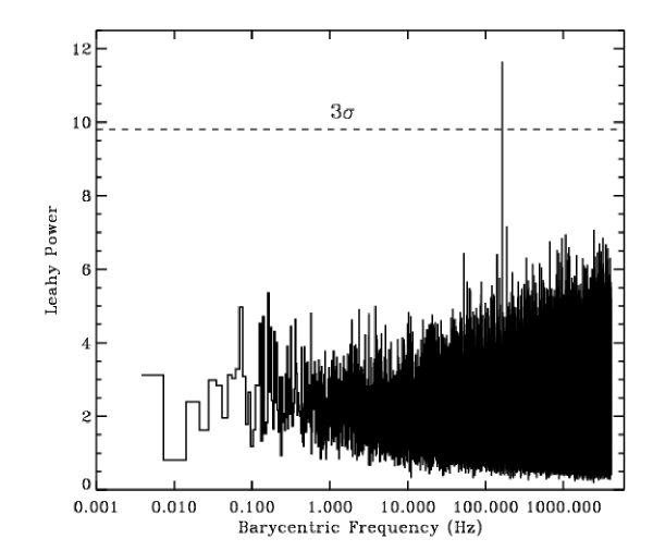
Figure 2.— Power spectrum of IGR J17062$-$6143 as a function of frequency (Barycentric) computed from 2 to 12 keV events and rebinned by a factor of 8. The 163.65 Hz pulsar peak is evident just above 100 Hz. The horizontal dashed line indicates the $3\sigma$ detection level. See §2 for a detailed discussion of the pulsation search.

Figure 3.— Dynamic power spectrum computed from 2 to 12 keV events. Contours as a function of time and frequency are drawn at Leahy power values of 20, 22, 24, 26, 28, 30, 32, 36, and 40. We used 512 s intervals to compute power spectra, and computed a new spectrum by sliding the interval by 16 s. The contours are drawn at the times corresponding to the center of each interval used to compute a power spectrum. Dashed vertical lines appear at 256 s and $T_{obs}$-256 s, marking the centers of the first and last intervals used to compute spectra, respectively. Time zero corresponds to 12:58:39.866 UTC on 2008 May 3.

Figure 4.— Results of coherent phase timing analysis. Phase residuals (cycles) vs. time from two different models for the frequency (and phase) evolution are shown. The black squares show the best-fitting, constant frequency model, which does not provide a good fit to the data, and shows a systematic trend indicative of spin-down of the pulsation frequency. The red symbols show a statistically acceptable circular orbit model with a period of 30 minutes. Time zero corresponds to 12:58:39.866 UTC on 2008 May 3.

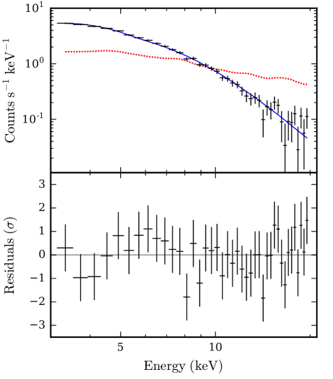
Figure 5.— PCA spectrum as a function of energy and the best-fitting absorbed power-law model (top; model in blue). The background (red curve) dominates the signal at high energies. A broad excess around $6$ keV is visible in the fit residuals (bottom), which may be due to photoionized reflection.