Approximate Bayes learning of stochastic differential equations

Abstract

We introduce a nonparametric approach for estimating drift and diffusion functions in systems of stochastic differential equations from observations of the state vector. Gaussian processes are used as flexible models for these functions and estimates are calculated directly from dense data sets using Gaussian process regression. We also develop an approximate expectation maximization algorithm to deal with the unobserved, latent dynamics between sparse observations. The posterior over states is approximated by a piecewise linearized process of the Ornstein-Uhlenbeck type and the maximum a posteriori estimation of the drift is facilitated by a sparse Gaussian process approximation.

I Introduction

Dynamical systems in the physical world evolve in continuous time and often the (noisy) dynamics is described naturally in terms of (stochastic) differential equations Gardiner:1996:HSM . However, due to missing information and/or the complexity of a system it may be difficult to derive such a model from first principles. Instead, the goal often is to fit it to observations of the state at discrete points in time Iacus:2008:SIS . So far most inference approaches for these systems have dealt with the estimation of parameters contained in the drift function (e.g. Wu:2011:BFM using a generalized linear model of locally linear forces or Golightly:2010:MCM using a Markov Chain Monte Carlo sampler), which governs the deterministic part of the microscopic time evolution. Assumptions for the stochastic part were often simple: additive noise with the diffusion constant as the only parameter to estimate. But as both drift and diffusion can be nonlinear functions of the state vector, a nonparametric estimation would be a natural generalization, when a large number of data points is available. Previous nonparametric approaches were based on solving the adjoint Fokker-Planck equation Lade:2009:FSI and on kernel estimators Bandi:2003:FNE and are effectively restricted to one-dimensional models.

An alternative would be a Bayesian nonparametric approach, where prior knowledge on the unknown functions—such as smoothness, variability, or periodicity—can be encoded in a probability distribution. A recent result by Papaspiliopoulos:2012:NED ; Pokern:2013:PCP presented an important step in this direction. The authors have shown that Gaussian processes (GPs) provide a natural family of prior probability measures over drift functions. If a path of the stochastic dynamics is observed densely, the posterior process over the drift is also a GP. Unfortunately, this simplicity is lost, when observations are not dense, but separated by larger time intervals. In Papaspiliopoulos:2012:NED the case of sparse observations has been treated by a Monte Carlo approach, which alternates between sampling complete diffusion paths of the stochastic differential equation (SDE) and sampling from GP for the drift given a path. A nontrivial problem is the sampling from SDE paths conditioned on observations. A second problem stems from the matrix inversions required by the GP predictions. For a densely sampled hidden path these matrices become large which leads to a strong increase in computational complexity. It was shown in Papaspiliopoulos:2012:NED for the case of univariate SDE that this numerical problem can be circumvented if one chooses a GP prior where the inverse of the covariance operator is specified as a differential operator. In this case efficient predictions are possible in terms of solutions of ordinary differential equations. Recently vanderMeulen:2014:RJM introduced a nonparametric method, which models the drift as linear combination of variably many basis functions and uses reversible-jump Markov chain Monte Carlo to sample from the posterior distribution. However, both vanderMeulen:2014:RJM and Papaspiliopoulos:2012:NED are restricted to one-dimensional SDEs. For special cases, where the drift of the system can be expressed as gradient of a potential, Batz:2016:VED uses the relationship between stationary density and potential in order to efficiently learn the drift based on the empirical density of the SDEs.

In this paper, we develop an alternative approximate method for Bayesian estimation of SDEs based on GPs. The method is faster than the sampling approach and can be applied to GPs with arbitrary covariance kernels and also multivariate SDEs. Also, our method is able to handle non-equilibrium models. In case of dense observations the framework of GP regression is used to estimate both drift and diffusion in a nonparametric way. For sparse observations, we use an approximate expectation maximization (EM) Dempster:1977:MLI algorithm, which extends our approach introduced in the conference publication Ruttor:2013:AGP . The EM algorithm cycles between the computation of expectations over SDE paths which are approximated by those of a locally fitted linear model and the computation of the maximum posterior GP prediction of the drift. In addition, the problem of the continuum of function values occurring in expectations over the hidden path is solved by a sparse GP approximation.

The paper is organized as follows. Stochastic differential equations are introduced in section II and Gaussian processes in section III. Then section IV explains GP based inference for completely observed paths and shows results on dense data sets. As large data sets slow down standard GP inference considerably, section V reviews an efficient sparse GP method. In section VI our approximate EM algorithm is derived and its performance is demonstrated on a variety of SDEs. Section VII presents a discussion and concludes with an outline of possible extensions to the method.

II Stochastic differential equations and likelihoods for dense observations

We consider diffusion processes given by a stochastic differential equation (SDE) written in Ito form as

$$dX_{t}=f(X_{t})dt+D^{1/2}(X_{t})dW_{t},$$ (1)

where the vector function $f(x)=(f^{1}(x),\ldots,f^{d}(x))$ defines the deterministic drift depending on the current state $X_{t}\in\mathcal{R}^{d}$. $W_{t}$ denotes a Wiener process, which models white noise, and $D(x)$ is the $d\times d$ diffusion matrix.

Suppose we observe a path $X_{0:T}$ of the process over a time interval $[0,T]$. Our goal is to estimate the drift function $f(x)$ based on the information contained in $X_{0:T}$. A well known statistical approach to estimation of unknown model parameters is the method of maximum likelihood Iacus:2008:SIS . This would maximize the probability of the observed path with respect to $f$. To derive an expression for such a path probability, we use the Euler time discretization of the SDE Kloeden:2011:NSS given by

$$X_{t+\Delta t}-X_{t}=f(X_{t})\Delta t+D(X_{t})^{1/2}\sqrt{\Delta t}\,\epsilon_{t},$$ (2)

where $\epsilon_{t}\sim\mathcal{N}(0,I)$ is a sequence of i.i.d. Gaussian noise vectors and $\Delta t$ is a time discretization. We will later set $\Delta t\to 0$, when we compute explicit results for estimators. Since the short time transition probabilities of the process are Gaussian, the probability density for the discretized path can be written as the product

$$p(X_{0:T}|f)=p_{0}(X_{0:T})L(X_{0:T}|f),$$ (3)

where

$$p_{0}(X_{0:T})\propto\exp\left[-\frac{1}{2\Delta t}\sum_{t}\left|\left|X_{t+\Delta t}-X_{t}\right|\right|^{2}\right]$$ (4)

is the measure over paths without drift, and a term

$$L(X_{0:T}|f) = \exp\Bigg{[}-\frac{1}{2}\sum_{t}\left|\left|f(X_{t})\right|\right|^{2}\Delta t$$ (5)

$$+ \left(f(X_{t}),X_{t+\Delta t}-X_{t}\right)\Bigg{]},$$

which is the relevant term for estimating the function $f$ from the observations of the path. To avoid cluttered notation, we have introduced the inner product $(u,v)\doteq u^{\top}D^{-1}v$ and the corresponding squared norm $||u||^{2}\doteq u^{\top}D^{-1}u$. The estimation of $f$ using the method of maximum likelihood can be motivated by the following heuristics: Consider the case of a very large observation time $T$. In this limit we may write

$$- \frac{1}{T}\ln L(X_{0:T}|f)$$ (6)

$$= \frac{1}{2T}\sum_{t}||f(X_{t})||^{2}\Delta t-2\left(f(X_{t}),X_{t+\Delta t}-X_{t}\right)$$

$$\simeq \frac{1}{2}\int_{0}^{T}\mathrm{E}\left[||f(X_{t})||^{2}\right]-2\mathrm{E}\left[\left(f(X_{t}),f_{*}(X_{t})\right)\right]dt$$

$$= \frac{1}{2}\int||f(x)||^{2}p(x)dx-\int\left(f(x),f_{*}(x)\right)p(x)dx,$$

where we have taken the limit $\Delta t\to 0$. The expectations are defined with respect to the true (but unknown) process from which the data points are generated and $p(x)$ denotes its stationary density. The true drift is given by the conditional expectation

$$f_{*}(x)=\lim_{\Delta t\to 0}\frac{1}{\Delta t}\mathrm{E}\left[X_{t+\Delta t}-X_{t}\middle|X_{t}=x\right].$$ (7)

Obviously, a minimization of the last term in (6) would lead to the estimator $\hat{f}(x)=f_{*}(x)$, which is the true drift indicating that asymptotically, for a long sequence of data we get a consistent estimate. Unfortunately, for finite sample time $T$, an unconstrained maximization of the likelihood (5) does not lead to sensible results Papaspiliopoulos:2012:NED . One has to use a regularization approach which restricts the complexity of the drift function. The simplest possibility is to work with a parametric model, e.g. representing $f$ by a polynomial and estimating its coefficients. However, in many cases it may not be clear in advance how many parameters such a model should have.

III Bayesian estimation with Gaussian processes

Another possibility for regularization is a nonparametric Bayesian approach which uses prior probability distributions $P_{0}(f)$ over drift functions. With different choices of the prior different statistical ensembles of typical drift functions can be selected. We denote probabilities over the drift $f$ by upper case symbols in order to avoid confusion with path probabilities. We will also denote expectations over functions $f$ by the symbol $\mathrm{E}_{f}$. Our Bayes estimator will be based on the posterior distribution

$$p(f|X_{0:T})\propto P_{0}(f)L(X_{0:T}|f),$$ (8)

where the neglected constant of proportionality only contains terms which do not depend on $f$. To construct such a prior distribution, we note that the exponent in (5) contains the drift $f$ at most quadratically. Hence a natural (conjugate) prior to the drift for this model is given by a Gaussian measure over functions, i.e. a Gaussian process (GP) Papaspiliopoulos:2012:NED . Although a more general model is possible, we will restrict ourselves to the case where the GP priors over the components $f^{j}(x)$, $j=1,\ldots,d$ of the drift factorize and we also assume that we have a diagonal diffusion matrix $D(x)=\mathrm{diag}(D^{1}(x),\ldots,D^{d}(x))$. In this case, the GP posteriors of $f^{j}(x)$ also factorize in the components $j$, and we can estimate drift components independently.

Gaussian processes have become highly popular in Bayesian statistics especially for applications within the field of machine learning Rasmussen:2006:GPM . Such processes are completely defined by a mean function $m(x)=\mathrm{E}_{f}[f(x)]$ (which we will set to zero throughout the paper) and a kernel function defined as

$$K(x_{1},x_{2})=\mathrm{E}_{f}[f(x_{1})f(x_{2})],$$ (9)

which specifies the correlation of function values at two arbitrary arguments $x_{1}$ and $x_{2}$. By the choice of the kernel $K$ we can encode prior assumptions about typical realizations of such random functions.

In this paper we will apply Gaussian processes not only to drift estimation but also to the estimation of the diffusion $D(x)$. The application in the latter case cannot be entirely justified from a Bayesian probabilistic perspective, but rather from the point of view that Gaussian processes are known to provide flexible tools for nonparametric regression, even when the underlying probabilistic model is not fully correctly specified. We will give a heuristic derivation of the analytical results for predictions with Gaussian processes which is applicable to both drift and diffusion estimation. A more detailed formulation can be found in Rasmussen:2006:GPM . In the basic regression setting, we assume that we have a set of $n$ input-output data points $(x_{i},y_{i})$ for $i=1,\ldots,n$, where the $y_{i}$ are modelled as noisy function values $f(X_{i})$, i.e.

$$y_{i}=f(x_{i})+\nu_{i},$$ (10)

where the noise values $\nu_{i}$, are taken to be independent Gaussian random variables with zero mean and (possibly different) variances $\sigma_{i}^{2}$. For drift estimation we take $f(x)\equiv f^{j}(x)$ as an arbitrary component of the drift vector and setting $D(x)\equiv D^{j}(x)$. We then identify

$$y_{i} = (X_{t_{i}+\Delta t}-X_{t_{i}})/\Delta t$$ (11)

$$\sigma_{i}^{2} = \frac{D(x_{t_{i}})}{\Delta t}.$$ (12)

In this case, the assumption of Gaussian noise is indeed fulfilled. Using a GP prior over functions $f$, we try to filter out the noise from the observations and learn to predict the unobserved function $f(x)$ at arbitrary input values $x$. For the drift estimation problem, this equals the conditional expectation

$$f(x)=\mathrm{E}[X_{t+\Delta t}-X_{t}|X_{t}=x]/\Delta t$$ (13)

for $\Delta t\to 0$. We will discuss the diffusion estimation problem in the next section, but mention that the noise $\nu_{i}$ will be no longer Gaussian. But we will still assume that GP regression will be able to estimate a conditional expectation of the type (10) in this case.

The probabilistic model for regression (10) corresponds to a likelihood

$$p(\mathbf{y}|f)\propto\exp\Bigg{[}-\sum_{i=1}^{n}\frac{1}{2\sigma_{i}^{2}}\left(f(x_{i})-y_{i}\right)^{2}\Bigg{]}\ ,$$ (14)

It is easy to see, that this likelihood agrees with (3) for the case of drift estimation. To compute the most likely function $f$ in the Bayesian sense, we minimize the negative log-posterior functional given by

$$- \ln\left[P_{0}(f)p(\mathbf{y}|f)\right]$$ (15)

$$\simeq \frac{1}{2}\int\int f(x)K^{-1}(x,x^{\prime})f(x^{\prime})dx\;dx^{\prime}$$

$$+\sum_{j=1}^{n}\frac{1}{2\sigma_{i}^{2}}(f(x_{j})-y_{j})^{2}.$$

Here $K^{-1}$ is the formal inverse of the kernel operator. Setting the functional derivative

$$\frac{\delta\ln\left[P_{0}(f)L(X_{0:T}|f)\right]}{\delta f(x)}=0$$ (16)

and applying the kernel operator $K$ to the resulting equation we get

$$f(x)=\sum_{j=1}^{n}\frac{\left(y_{j}-f(x_{j})\right)}{\sigma_{j}^{2}}K(x,x_{j}).$$ (17)

Evaluating this equation at observation $x=x_{i}$ we obtain

$$\frac{(y_{i}-f(x_{i}))}{\sigma_{i}^{2}}=\left(\left(\mathbf{K}+\boldsymbol{\Sigma}\right)^{-1}\mathbf{y}\right)_{i}.$$ (18)

Here $\mathbf{K}=(K(x_{i},x_{j}))_{i,j=1}^{n}$ denotes the kernel matrix and $\boldsymbol{\Sigma}=\mathrm{diag}(\sigma^{2}_{1},\ldots,\sigma^{2}_{n})$ is a diagonal matrix composed of the noise variances at the data points. This yields the following expression (see Rasmussen:2006:GPM ) for the GP estimator of the function $f$:

$$\hat{f}(x)=(\mathbf{k}(x))^{\top}\left(\mathbf{K}+\boldsymbol{\Sigma}\right)^{-1}\mathbf{y},$$ (19)

where $\mathbf{k}(x)=(K(x,x_{i}))^{\top}$. Specializing to the estimation of the j-th drift component we identify $\mathbf{y}=((X_{t+\Delta t}-X_{t})/\Delta t)^{\top}$ and $\boldsymbol{\Sigma}=\mathbf{D}^{j}/\Delta t$, where $\mathbf{D}^{j}$ is diagonal matrix composed of the diffusions $D^{j}(x_{i})$ for $i=1,\ldots,n$, to get

$$\hat{f}^{j}(x)=(\mathbf{k}(x)^{j})^{\top}\left(\mathbf{K}^{j}+\frac{1}{\Delta t}\mathbf{D}^{j}\right)^{-1}\!\!\!\!\!\!\mathbf{y}^{j},$$ (20)

where $\mathbf{k}(x)^{j}=(K(x,x_{i})^{j})^{\top}$. A similar approach leads to the Bayesian uncertainty at $x$,

$$\qquad\hat{D}_{f^{j}}(x)=K(x,x)^{j}-(\mathbf{k}(x)^{j})^{\top}\left(\mathbf{K}^{j}+\frac{1}{\Delta t}\mathbf{D}^{j}\right)^{-1}\!\!\!\!\!\!\mathbf{k}(x)^{j},$$ (21)

which can be used to quantify the uncertainty of the prediction.

A popular covariance kernel is the radial basis function (RBF) kernel

$$K_{\tiny{RBF}}(x_{1},x_{2})=\tau^{2}_{\mathrm{RBF}}\exp\left(-\frac{||x_{1}-x_{2}||^{2}}{2l_{\mathrm{RBF}}^{2}}\right),$$ (22)

where the hyperparameters $\tau^{2}_{\mathrm{RBF}}$ and $l_{\mathrm{RBF}}$ denote the variance and the correlation length scale of the process. The RBF kernel assumes smooth, infinitely differentiable functions $f(\cdot)$. In some cases, the class of functional relationship in the data set is known beforehand, so that specialized kernel functions encoding this prior information can be applied. In our experiments, we use such kernels for the estimation of polynomial and periodic functions $f(\cdot)$. The corresponding kernels are the polynomial kernel of degree $p$,

$$K_{\tiny{Pol}}(x_{1},x_{2})=\left(1+x_{1}^{\top}x_{2}\right)^{p},$$ (23)

and the (one-dimensional) periodic kernel

$$K(x_{1},x_{2})_{\mathrm{Per}}=\tau_{\mathrm{Per}}^{2}\exp\left(-\frac{2\sin\left(\frac{x_{1}-x_{2}}{2}\right)^{2}}{l_{\mathrm{Per}}^{2}}\right).$$ (24)

For the latter kernel, the hyperparameters $\tau^{2}_{\mathrm{Per}}$ and $l_{\mathrm{Per}}$ denote the variance and the correlation length scale of the process.

In our experiments we found that the choice of the variance kernel parameter $\tau$ did not have a noticeable impact on the estimation results. Consequently, we fixed its value to $\tau=1$. In the case of the length scale hyperparameter $l$ the user usually has relevant prior expert knowledge about the specific problem at hand and is able to determine its value a priori. Similarly, if one knows that the underlying problem is of polynomial form, one should be able to specify its order $p$ or at least an upper bound for $p$. We found that this approach usually works well in practice. We note, however, that in the case of dense data the kernel hyperparameters can also be automatically determined in a principled way (see section IV).

Figure 1: Sample path with $n=6000$ data points generated from a double well model with time distance $\Delta_{t}=0.002$.

Figure 2: (color online) Estimation for the double well model based on the direct GP with the solid black line denoting the mean and the dashed red line the true drift function.

Figure 3: (color online) Diffusion estimation of the double well based on the direct GP. The dashed red line denotes the square root of the diffusion $D(x)^{1/2}$ and the solid black line the estimator.

IV Estimation for dense observations

Following the dense case of section III, we consider drift and diffusion estimation in cases where the time grid $\Delta t$ on which the data points are observed is small. This approach will be referred to as the direct Gaussian Process (GP) estimation with mean and variance given by (20) and (21), respectively. We will treat drift and diffusion estimation in turn and start with the latter. The order is motivated by the fact that the diffusion estimation is independent of the drift. Hence, if both drift and diffusion are unknown, one should first learn the diffusion and then incorporate the estimation results into the drift learning procedure.

IV.1 Diffusion Estimation

We distinguish between two cases, namely models with constant and with state dependent diffusion. If the diffusion matrix $D$ is known to be constant, i.e. it does not depend on the state, we will use a Bayesian maximum likelihood approach and optimize the so-called Bayes evidence, which equals the probability of the path $p(X_{0:T})$ (in its Euler discretization), with respect to the diffusion constants $D=(D^{1},\ldots,D^{d})$. Again the probability factorizes in the components $j=1,\ldots,d$. For component $j$ of the process, the evidence is defined as the $n$-dimensional Gaussian integral

$$p(X^{j}_{0:T})=\int p(X^{j}_{0:T}|\mathbf{f}^{j})p_{0}(\mathbf{f}^{j})d\mathbf{f}^{j}$$ (25)

where $\mathbf{f}^{j}$ denotes the vector with components $f^{j}(X_{t_{i}})$ for $i=1,\ldots,n$ and $p_{0}(\mathbf{f}^{j})=\mathcal{N}(\mathbf{f}^{j}|\mathbf{0},\mathbf{K}^{j})$ is the prior Gaussian density induced by the GP prior over functions. Introducing, as before, the notation $y^{j}_{i}=(X^{j}_{t_{i}+\Delta t}-X^{j}_{t_{i}})/\Delta t$, we easily obtain the closed form expression

$$p(X^{j}_{0:T})=\mathcal{N}(\mathbf{y}^{j}|\mathbf{0},\mathbf{K}^{j}+\boldsymbol{\Sigma}^{j}).$$ (26)

from (25) with $\boldsymbol{\Sigma}^{j}=(D^{j}/\Delta t)\mathbf{I}$, and where $\mathbf{I}$ denotes the identity matrix. For the optimization, one can use a standard routine, e.g. a quasi-Newton method. The evidence can also be used in the same way to learn kernel hyperparameters by optimizing with respect to the specific variables.

In the case of state dependent diffusions $D(x)$, the evidence optimization becomes impractical, since we would have to jointly optimize over $D(x_{i})$ for all $N$ observations. Instead, we use the well known representation Gardiner:1996:HSM for an arbitrary component of the exact diffusion

$$D^{*}(x) =\lim_{\Delta t\to 0}\frac{1}{\Delta t}\mathrm{Var}\left(X_{t+\Delta t}-X_{t}|X_{t}=x\right)$$

$$=\lim_{\Delta t\to 0}\frac{1}{\Delta t}\left(\mathrm{E}\left[(X_{t+\Delta t}-X_{t})^{2}|X_{t}=x\right]\right.$$

$$\quad\qquad\qquad\left.-\mathrm{E}\left[X_{t+\Delta t}-X_{t}|X_{t}=x\right]^{2}\right)$$ (27)

$$=\lim_{\Delta t\to 0}\frac{1}{\Delta t}\left(\mathrm{E}\left[(X_{t+\Delta t}-X_{t})^{2}|X_{t}=x\right]\right.$$

$$\quad\qquad\qquad\left.-\mathrm{E}[\Delta tf^{*}(x)]^{2}\right)$$

$$=\lim_{\Delta t\to 0}\frac{1}{\Delta t}\mathrm{E}\left[(X_{t+\Delta t}-X_{t})^{2}|X_{t}=x\right].$$ (28)

In the third line, we use the fact that the second term on the right hand side equals the squared conditional drift (7). Then—by taking $\Delta t$ out of the expectation $\mathrm{E}[\Delta tf^{*}(x)]$—we can easily see that the term vanishes in the limit $\Delta t\to 0$. Hence, the conditional variance does not depend on the drift. For its computation, we use again GP regression, but now on the data set $((x_{1},\tilde{y}_{1}),\ldots,(x_{n},\tilde{y}_{n}))$, where $\tilde{y}_{i}=(X_{t_{i}+\Delta t}-X_{t_{i}})^{2}/\Delta t$ are proportional to the squared observations of the drift estimation problem.

Unfortunately, the data $\mathbf{\tilde{y}}$ do not follow a Gaussian distribution, so interpreting the GP posterior as a Bayesian posterior would lead to a model mismatch. Trying to work with the exact likelihood would lead to intractable non-Gaussian integrals involving Gamma-densities which would have to be approximated. Moreover, the noise in the data $\tilde{y}_{i}$ depends itself on the diffusion $D(x_{i})$ and a proper Bayesian treatment would lead to a more complicated iterative estimation problem. However, the observations $\mathbf{\tilde{y}}^{j}$ are obviously much smoother than the $\mathbf{y}^{j}$. Hence, we expect that the following simpler heuristics gives good results for densely sampled paths. We regard the GP framework simply as a regression tool for function estimation, which in our case happens to be the diffusion function. The regression curve is given by the GP mean (19) with $\mathbf{y}^{j}$ substituted by $\mathbf{\tilde{y}}^{j}$. Note that this is conceptually different from the computation of the constant diffusion case above, where we matched the likelihood variances $\hat{\sigma}_{j}^{2}$ to the diffusion estimators $\hat{D}^{j}$ of the process. Under the GP as a regression toolbox lense, the likelihood variance $\sigma^{2}$ becomes a nuisance parameter without a direct interest to us. Still, we have to determine suitable variance values as well as possibly length scale parameters in the case of a RBF kernel, which might not be readily available.

Finding hyperparameters by optimizing the marginal distribution presupposes a Bayesian interpretation and so is not applicable in this context. Therefore we resort to a 2-fold cross-validation scheme. This method randomly divides the observation into two subsets of equal size, and learns a GP estimator on each of the subsets. Then the goodness of fit is determined by computing the mean squared error of each estimator on the data of the remaining subset.

IV.2 Drift Estimation

Once we have diffusion values at the observations at our disposal, the estimation of the drift function becomes straightforward. All we have to do is to evaluate for each component $j$ the diffusion at the observations $\mathbf{D}^{j}(x)$, which we then use as GP variance in the drift estimation. For the constant but unknown diffusion model, we insert the estimated value $\hat{D}^{j}$ into the diagonal of the matrix $\mathbf{D}^{j}$, in the state dependent unknown diffusion model, we use the estimated value $\hat{D}^{j}(x_{i})$ from the diffusion regression function described above. Then, running the direct GPs on the observations $\mathbf{y}^{j}$ leads to a drift estimation, which can once again be interpreted as Bayesian posterior. However, we emphasize that we again regard the GP as regression toolbox for computing an expectation function.

IV.3 Experiments

Here we show the results for two experiments with unknown state dependent diffusion. First we look at synthetic data and then at a real world data set used in climate research. The synthetic data sets analyzed are generated using the Euler method from the corresponding SDE with grid size $\Delta t=0.002$.

Double well model with unknown state dependent diffusion

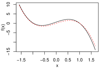
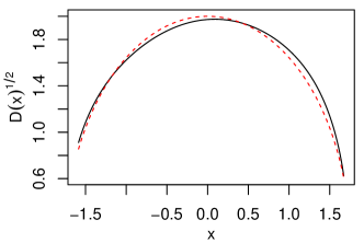
In order to evaluate the direct GP method, we generated a sample of size $n=5000$ with step size $\Delta t=0.002$ from the double well process Archambeau:2007:VID with state dependent diffusion:

$$dX=4(X-X^{3})dt+\sqrt{\max(4-1.25X^{2},0)}dW_{t}.$$ (29)

The direct GP was run with a polynomial kernel function of order $p=4$. The estimation for drift and diffusion function are given in figures 2 and 3, respectively. In both cases, we see a good fit between estimator and true function.

Ice core model

As an example of a real world data set, we used the NGRIP ice core data (provided by Niels-Bohr institute in Copenhagen, (Andersen:2004:HRR, ), which provides an undisturbed ice core record containing climatic information stretching back into the last glacial. Specifically, this data set as shown in figure 6 contains $4918$ observations of oxygen isotope concentration $\delta^{18}O$ over a time period from the present to roughly $1.23\cdot 10^{5}$ years into the past. Since there are generally less isotopes in ice formed under cold conditions, the isotope concentration can be regarded as an indicator of past temperatures.

Figure 4: (color online) The figure shows the estimated potentials of the ice core data both from a model with state dependent diffusion $D(x)$ (solid black line) and with constant diffusion $D$ (dotted red). For both models we use a RBF kernel with length scale $l=0.7$. The corresponding diffusion estimators are shown in figure 5.

Figure 5: (color online) Diffusion function estimators of the ice core model for the state dependent (solid black line) and the constant diffusion model (dotted red line). The constant value $D^{1/2}=2.81$ was found by optimization of the marginal likelihood. For the GP in the state dependent model we used a RBF kernel, whose length scale $l=2.71$ and diffusion $D=0.1$ was determined by 2-fold cross-validation.

Figure 6: (color online) Plot of the ice core data (as solid black line) with metastable states marked by dashed green lines. These four minima of the potential function were identified by the direct GP algorithm with state dependent diffusion.

Figure 7: (color online) Plot of the ice core drift function corresponding to the above potential function in black together with the 95%- Bayes confidence bounds shaded in blue. One can see that the two inner meta stable states are statistically significant, while the outer two ones are not.

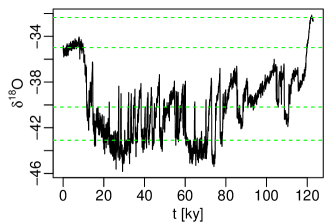
Recent research Kwasniok:2013:AMG suggest to model the rapid paleoclimatic changes exhibited in the data set by a simple dynamical system with a drift function of order $p=3$ as canonical model, which allows for bistability. This corresponds to a meta stable state at higher temperatures close to marginal stability and a stable state at low values, which is consistent with other research on this data set linking a stable state of oxygen isotopes to a baseline temperature and a region at higher values corresponding to the occurrence of rapid temperature spikes. For this particular dataset the consecutive observations are spaced $\Delta t=0.05\mathrm{ky}^{-1}$ apart. The underlying dynamics of the NGRIP data set is often modelled as a constant noise process in the literature (Kwasniok:2013:AMG, ).

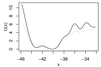
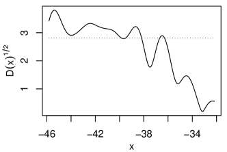
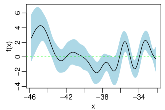
Figure 5 shows that the estimated diffusion function changes significantly over the range of the observed isotope concentration, which seems to make the constant diffusion assumption in the model of Kwasniok:2013:AMG inadequate. Our data-driven approach not only reveals this multiplicative nature of the noise, but also a richer structure of the learnt potential in comparison to the potential function of the constant diffusion model, as shown in figure 4. Hence, choosing a state dependent diffusion model is advisable even in cases where one is only interested in the potential, since the noise structure of the data also influences the estimation of the potential (and drift) function.

Here we find in total four local minima, but only two would be expected for a polynomial drift of order $p=3$. Switches between the two lowest states at $\delta^{18}O\approx-43.1$ and $\delta^{18}O\approx-40.2$ occur quite frequently due to a low barrier and high diffusion. A more obvious metastable state is found at $\delta^{18}O\approx-35.0$ because of an asymmetric barrier and lower noise levels. As there are only a few data points available around $\delta^{18}O=-32.4$, this metastable state is not statistically significant in the estimate of the drift function shown in figure 7.

V Large Number of observations: The need for a sparse GP

In practice, the number of observations can be large for a fine time discretization, and a fast computation of the matrix inverses in (20) could become infeasible. A possible way out of this problem—as suggested by Papaspiliopoulos:2012:NED —could be a restriction to kernels for which the inverse kernel is a differential operator. We will now resort to a different approach which applies to arbitrary kernels and generalizes easily to multivariate SDE. Our method is based on a variational approximation to the GP posterior Titsias:2009:VLI ; Csato:2002:TGF , where the likelihood term of the GP model (5) is replaced by another effective likelihood, which depends only on a smaller set of variables $\mathbf{f}_{s}$.

V.1 The general case

We assume a collection of random variables $f=\{f(x)\}_{x\in T}$ where the index variable $x\in T$ takes values in some possibly infinite index set $T$. We will assume a prior measure denoted by $P_{0}(f)$ and a posterior measure of the form

$$P(f)=\frac{1}{Z}P_{0}(f)\;e^{-U(f)},$$ (30)

where $U(f)$ is a functional of $f$. The goal is to approximate $P$ by another measure $Q$ of the form

$$Q(f)=\frac{1}{Z_{s}}P_{0}(f)\;e^{-U_{s}(\mathbf{f}_{s})},$$ (31)

where the potential $U_{s}$ depends only on a smaller sparse set $\mathbf{f}_{s}=\{f(x)\}_{x\in S}$ of dimension $m$. $S$ is not necessarily a subset of $T$. While we keep the set $S$ fixed, $U_{s}$ will be optimized to minimize the variational free energy of the approximation

$$-\ln Z\leq-\ln Z_{s}+\mathrm{E}_{s}\left[U(f)-U_{s}(\mathbf{f}_{s})\right].$$ (32)

We write the joint probability of $\mathbf{f}$ and $\mathbf{f}_{s}$ as

$$Q(f,\mathbf{f}_{s})=Q(f|\mathbf{f}_{s})Q(\mathbf{f}_{s})=P_{0}(f|\mathbf{f}_{s})Q(\mathbf{f}_{s}),$$ (33)

where the last equality follows from the fact that fixing the sparse set $\mathbf{f}_{s}$, $U(\mathbf{f}_{s})$ becomes non-random and the dependency on the random variables $f$ is only via $P_{0}$ and we have

$$Q(\mathbf{f}_{s})=\frac{P_{0}(\mathbf{f}_{s})}{Z_{s}}\;e^{-U_{s}(\mathbf{f}_{s})}.$$ (34)

Hence, we can integrate out all variables $f$ except $\mathbf{f}_{s}$ using $P_{0}(f|\mathbf{f}_{s})$ and rewrite the variational bound as the finite dimensional integral

$$-\ln Z \leq -\ln Z_{s}+\int Q(\mathbf{f}_{s})\left\{\mathrm{E}_{0}[U(f|\mathbf{f}_{s})]-U_{s}(\mathbf{f}_{s})\right\}d\mathbf{f}_{s}$$ (35)

$$= \int Q(\mathbf{f}_{s})\ln\left(\frac{Q(\mathbf{f}_{s})}{P_{0}(\mathbf{f}_{s})\;e^{-\mathrm{E}_{0}[U(f|\mathbf{f}_{s})]}}\right)d\mathbf{f}_{s}.$$

$\mathrm{E}_{0}[U(f|\mathbf{f}_{s})]$ is the conditional expectation w.r.t. $P_{0}$. Since this is of the form of a relative entropy, we conclude that the bound is minimized by the choice

$$Q(\mathbf{f}_{s})\propto P_{0}(\mathbf{f}_{s})e^{-\mathrm{E}_{0}[U(f|\mathbf{f}_{s})]}$$ (36)

and thus $U_{s}(\mathbf{f}_{s})=\mathrm{E}_{0}[U(f|\mathbf{f}_{s})]$.

V.2 Gaussian random variables

We next specialize to a Gaussian measure $P_{0}$ with zero mean and covariance kernel $K$. If we assume (for notational simplicity) that the set $\{f\}$ is represented as a finite but high-dimensional vector $\mathbf{f}$ and

$$U(\mathbf{f})=\frac{1}{2}\mathbf{f}^{\top}\mathbf{A}\mathbf{f}-\mathbf{b}^{\top}\mathbf{f}$$ (37)

is a quadratic form, we can then further simplify the conditional expectation (36) to

$$\mathrm{E}_{0}[U(\mathbf{f})|\mathbf{f}_{s}] = \frac{1}{2}(\mathrm{E}_{0}[\mathbf{f}|\mathbf{f}_{s}])^{\top}\mathbf{A}\mathrm{E}_{0}[\mathbf{f}|\mathbf{f}_{s}]$$ (38)

$$- \mathbf{b}^{\top}\mathrm{E}_{0}[\mathbf{f}|\mathbf{f}^{s}]+C,$$

where

$$C=\frac{1}{2}\mathrm{tr}\left(\mathrm{Cov}_{0}[\mathbf{f}|\mathbf{f}_{s}]\mathbf{A}\right)$$ (39)

is a constant independent of $\mathbf{f}_{s}$. This follows from the fact that $\mathrm{E}_{0}[\mathbf{f}|\mathbf{f}_{s}]$ is the optimal mean square predictor of the vector $\mathbf{f}$ given $\mathbf{f}_{s}$ Papoulis:1965:PRV , the difference $\mathbf{f}-\mathrm{E}_{0}[\mathbf{f}|\mathbf{f}_{s}]$ is a random vector which is uncorrelated to the vector $\mathbf{f}_{s}$ and thus for jointly Gaussian random variables independent of $\mathbf{f}_{s}$. Hence the conditional covariance $\mathrm{Cov}_{0}$ of $\mathbf{f}$ does not depend on $\mathbf{f}_{s}$. The explicit result for this predictor is given by

$$\mathrm{E}_{0}[\mathbf{f}|\mathbf{f}^{s}]=\mathbf{K}_{Ns}\mathbf{K}_{s}^{-1}\mathbf{f}_{s},$$ (40)

where $\mathbf{K}_{s}$ is the kernel matrix for the sparse set and $\mathbf{K}_{Ns}$ is the $n\times m$ kernel matrix between the non-sparse and the sparse set. It is now easy to generalize to the infinite dimensional case of the form

$$U(f)=\frac{1}{2}\int f^{2}(x)A(x)dx-\int f(x)b(x)dx,$$ (41)

for which we get

$$\mathrm{E}_{0}[f(x)|\mathbf{f}_{s}]=\mathbf{k}_{s}^{\top}(x)(\mathbf{K}_{s})^{-1}\mathbf{f}_{s}$$ (42)

and thus

$$\mathrm{E}_{0}[U(\mathbf{f})|\mathbf{f}_{s}] = \frac{1}{2}\mathbf{f}_{s}^{\top}\mathbf{K}_{s}^{-1}\left\{\int\mathbf{k}_{s}(x)\;A(x)\;\mathbf{k}_{s}^{\top}(x)dx\right\}\mathbf{K}_{s}^{-1}\mathbf{f}_{s}$$ (43)

$$- \mathbf{f}_{s}^{\top}\mathbf{K}_{s}^{-1}\int\mathbf{k}_{s}(x)\;b(x)\;dx.$$

V.3 Sparse GP Drift and Diffusion Estimation

Now, setting

$$U(f)=-\ln[L(X_{0:T}\mid f)],$$ (44)

we can derive the drift estimator for the sparse representation analogously to (15). With definitions $\boldsymbol{\pi}^{j}=\mathbf{K}_{Ns}^{j}\left(\mathbf{K}_{s}^{j}\right)^{-1}$ and $\Omega^{j}=\Delta t(\boldsymbol{\pi}^{j})^{T}\mathbf{D}^{-1}\boldsymbol{\pi}^{j}$ we get for the $j$th component of the drift vector:

$$\hat{f}^{j}(x)=(\mathbf{k}(x)^{j})^{\top}\left(\mathbf{I}+\Omega^{j}\mathbf{K}_{s}^{j}\right)^{-1}\Delta t(\boldsymbol{\pi}^{j})^{T}(\mathbf{D}^{j})^{-1}\mathbf{y}^{j},$$ (45)

where $\mathbf{k}(x)^{j}=(K(x,x_{i})^{j})^{\top}$.

The corresponding expression for the variance estimator is given by:

$$\hat{D}_{f^{j}}(x)=K(x,x)-\mathbf{k}(x)^{\top}\left(\mathbf{I}+\Omega^{j}\mathbf{K}_{s}^{j}\right)^{-1}\Omega^{j}\mathbf{k}(x).$$ (46)

Notice that the inverted matrix inside the drift and variance estimators is no longer of the size of observations $n\times n$, but of the size of the sparse set $m\times m$.

While it is possible to also optimize the approximation with respect to the set of sparse points numerically Csato:2002:SPG ; Rasmussen:2006:GPM , we use a simple heuristic, where we construct a histogram over the observations and select as our sparse set $S$ the midpoints of all histogram hypercubes containing at least one observation. Here, the intuition is that a sparse point in a region of high empirical density is a good approximation to the data points in the respective hypercube. The number of histogram bins is determined by Sturges’ formula Sturges:1926:CCI , which is implicitly based on the range of the data. Note that the cardinality $m$ of the sparse set is not set in advance but automatically determined by the spatial structure of the data. In practice, this heuristic typically leads to $m\ll n$ and therefore to substantial computational gains compared to the full GP.

In practice, using the sparse GP for the drift and diffusion function estimation can be easily accomplished by first determining a sparse set $S$ for the relevant data set and then substituting mean (20) and variance (21) equations with their sparse GP counterparts (45) and (46), respectively.

One exception is the estimation of the constant diffusion $\mathbf{D}$, where we have to replace the marginal distribution (25) with a corresponding sparse approximation. Here, we follow Titsias:2009:VLI and optimize for each component $j$ a lower bound to the evidence with respect to the diffusion constants:

$$F_{V}(X_{0:T}) =\log[\mathcal{N}(\mathbf{y}^{j}|\mathbf{0},\mathbf{Q}_{N}^{j}+\frac{1}{\Delta t}\mathbf{D}^{j})]$$

$$-\frac{\Delta t}{2}(\mathbf{D}^{j})^{-1}\mathrm{tr}(\mathbf{K}^{j}-\mathbf{Q}_{N}^{j}),$$ (47)

where $\mathbf{Q}_{N}^{j}=\mathbf{K}_{Ns}^{j}(\mathbf{K}_{s}^{j})^{-1}(\mathbf{K}_{Ns}^{j})^{T}$ and $\mathrm{tr}(\cdot)$ denotes the trace of the matrix.

V.4 Performance comparison

In order to get a feel for the performance differences between the standard GP and its sparse counterpart, we compare both versions in terms of accuracy and performance on the double well model

$$dX=4(X-X^{3})dt+D^{1/2}dW_{t}$$ (48)

with constant and known variance $D=1$. For the comparison, we analyzed the performance for data sets of different sizes, where we generated $10$ data sets with $\Delta t=0.002$ for each fixed number of observations. As accuracy measure, we used the approximate mean squared error (MSE)

$$\int p(z)(\hat{f}(z)-f(z))^{2}dz\approx\frac{1}{S}\sum_{i=1}^{S}(\hat{f}(z_{i})-f(z_{i}))^{2}$$ (49)

of the corresponding estimator. Here $\hat{f}(z)$ denotes the estimated drift and $f(z)$ the true drift value, each evaluated on a set of $S=100$ fixed points evenly spaced over the range of the samples. We then measured the run time and MSE of each data set based on the sparse GP and the standard GP estimation, each with a polynomial kernel of order $p=4$. All MSE are computed for one fixed test set of size $n=4000$, which we generated from the same model with $\Delta t=0.5$.

Table 1 shows the mean values of the run time and MSE for each fixed observation number, respectively. One can see that the sparse GP algorithm leads to a significant reduction in computing time while exhibiting practically no loss in estimation accuracy. As expected, the efficiency gain grows with larger data sets and even allows us to to analyze big data sets which are computationally infeasible for the standard GP method.

Sample	full GP	full GP	sparse GP	sparse GP
Size	Runtime	MSE	Runtime	MSE
300	0.077	1.507	0.005	1.507
500	0.104	1.384	0.008	1.384
1000	0.828	1.292	0.014	1.293
2500	4.19	1.157	0.028	1.157
5000	30.18	0.973	0.056	0.973
10000	324.5	0.592	0.162	0.593
50000	-	-	0.783	0.142

Table 1: Results of mean run times and MSEs of the standard GP and sparse GP algorithms for different sample sizes, run on a machine with Intel Core i3 processor. The size of the sparse sets varied between $m=6$ and $m=19$.

VI Estimation for sparse observations

The direct GP approach outlined above leads to wrong estimates of the drift when observations are sparse in time. In the sparse setting, we assume that $n$ observations $z_{k}\doteq X_{\tau_{k}}$, $k=1,\ldots,n$ are obtained at (for simplicity) regular intervals $\tau_{k}=k\tau$, where $\tau\gg\Delta t$ is much larger than the microscopic time scale. In this case, a straightforward discretization in (5), where the sum over microscopic times $t_{i}$ would be replaced by a sum over macroscopic times $\tau_{k}$ and $\Delta t$ by $\tau$, would correspond to a discrete time dynamical model of the form (1) again replacing $\Delta t$ by $\tau$. But this discretization is a bad approximation to the true SDE dynamics. This is because the transition kernel over macroscopic times $\tau$ is simply not a Gaussian for a general $f$ as was assumed in (15). The failure of the direct estimator for larger time distances can be seen in figure 9, where the red line corresponds to the true drift of the double-well (with constant, known diffusion) and the black line to its prediction based on observations with $\tau=0.2$.

Figure 8: (color online) Snippet of the double well sample path in black with observations denoted as red dots.

Figure 9: (color online) Estimated drift function for the double well based on the direct approach, where the red dashed line denotes the true drift function and the solid black line the mean function. One can clearly see that the larger distance between the consecutive points leads to a wrong prediction.

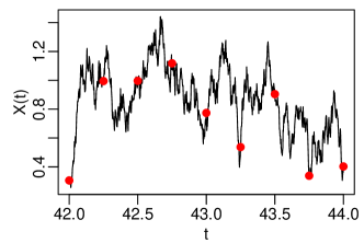
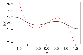
To deal with this problem, we treat the process $X_{t}$ for times $t$ between consecutive observations $k\tau<t<(k+1)\tau$ as a hidden stochastic process with a conditional path probability given by

$$p(X_{0:T}|\mathbf{z},f)\propto p(X_{0:T}|f)\prod_{k=1}^{n}\delta(z_{k}-X_{k\tau}),$$ (50)

where $\mathbf{z}$ is the collection of observations $z_{k}$. We will use an iterative method based on the EM algorithm Dempster:1977:MLI , in which the unobserved complete paths are replaced by an appropriate expectation using the probability (50).

VI.1 EM algorithm

The EM algorithm cycles between two steps

1. In the E-step, we compute the expected negative logarithm of the complete data likelihood

   $$\mathcal{L}(f,p)=-\mathrm{E}_{p}\left[\ln L(X_{0:T}|f)\right],$$ (51)

   where $p$ denotes the posterior $p(X_{0:T}|\mathbf{z},f_{old})$ for the previous estimate $f_{old}$ of the drift.

2. In the M-Step, we recompute the most likely drift function by the minimization

   $$f_{new}=\arg\min_{f}\left(\mathcal{L}(f,p)-\ln P_{0}(f)\right).$$ (52)

On can show Dempster:1977:MLI that the EM algorithm converges to a local maximum of the log-posterior. To compute the expectation in the E-step, we use (5) and take the limit $\Delta t\to 0$ at the end, when expectations have been computed. As $f(x)$ is a time-independent function, this yields

$$- \mathrm{E}_{p}\left[\ln L(X_{0:T}|f)\right]$$ (53)

$$= \lim_{\Delta t\to 0}\frac{1}{2}\sum_{t}\mathrm{E}_{p}\left[||f(X_{t})||^{2}\right]\Delta t$$

$$- 2\mathrm{E}_{p}\left[\left(f(X_{t}),X_{t+\Delta t}-X_{t}\right)\right]$$

$$= \frac{1}{2}\int_{0}^{T}\mathrm{E}_{p}\left[||f(X_{t})||^{2}\right]-2\mathrm{E}_{p}\left[\left(f(X_{t}),g_{t}(X_{t})\right)\right]dt$$

$$= \frac{1}{2}\int||f(x)||^{2}A(x)dx-\int\left(f(x),z(x)\right)dx.$$

We have defined the corresponding drift conditioned on data

$$g_{t}(x)=\lim_{\Delta t\to 0}\frac{1}{\Delta t}\mathrm{E}_{p}[X_{t+\Delta t}-X_{t}|X_{t}=x],$$ (54)

as well as the functions

$$A(x)=\int_{0}^{T}q_{t}(x)dt$$ (55)

and

$$b(x)\,=\int_{0}^{T}g_{t}(x)q_{t}(x)dt.$$ (56)

In contrast to (6), expectations are now over marginal densities $q_{t}(x)$ of $X_{t}$ computed from the conditional path measure, not over the asymptotic stationary density. Hence, we end up again with a simple quadratic form in $f$ to be minimized. Note that due to the smoothness of the kernel the prediction of (52) can be easily differentiated analytically, a fact that will be needed later.

However, there are two main problems for a practical realization of this EM algorithm:

• We can not compute the expectation with respect to the conditional path measures exactly and need to find approximations applicable to arbitrary prior drift functions $f(x)$.

• Although real observations are sparse, the hidden path involves a continuum of values $X_{t}$. This will require (e.g. after some fine discretization of time) the inversion of large matrices in (20).

We can readily deal with the latter problem by resorting to the sparse GP representation introduced in section V.

Linear drift approximation: The Ornstein-Uhlenbeck bridge

In this section we will look at the first problem of computing expectations in the E-step. For given drift $f(\cdot)$ and times $t\in I_{k}$ in the interval $I_{k}=[k\,\tau;(k+1)\tau]$ between two consecutive observations, the exact marginal $p_{t}(x)$ of the conditional path distribution equals the density of $X_{t}=x$ conditioned on the fact that $X_{k\tau}=z_{k}$ and $X_{(k+1)\tau}=z_{k+1}$ . This is a so-called diffusion bridge. Using the Markov property, this density can be expressed by the transition densities $p_{s}(x_{t+s}|x_{t})$ of the homogeneous Markov diffusion process with drift $f(x)$ as

$$p_{t}(x)\propto p_{(k+1)\tau-t}(z_{k+1}|x)p_{t-k\tau}(x|z_{k})\;\mbox{for}\;t\in I_{k}.$$ (57)

As functions of $t$ and $x$, the second factor fulfills a forward Fokker-Planck equation and the first one a Kolmogorov backward equation Gardiner:1996:HSM . Since exact computations are not feasible for general drift functions, we approximate the transition density $p_{s}(x|x_{k})$ in each interval $I_{k}$ by that of a homogeneous Ornstein-Uhlenbeck process Gardiner:1996:HSM , where the drift $f(x)$ is replaced by a local linearization. Hence, we consider the approximate process

$$dX_{t}=[f(z_{k})-\Gamma_{k}(X_{t}-z_{k})]dt+D^{1/2}_{k}dW$$ (58)

with $\Gamma_{k}=-\nabla f(z_{k})$ and $D_{k}=D(z_{k})$ for $t\in I_{k}$. For this process, the transition density is a multivariate Gaussian

$$q_{s}^{(k)}(x|z)=\mathcal{N}\left(x|\alpha_{k}+e^{-\Gamma_{k}s}(z-\alpha_{k});S_{s}\right),$$ (59)

where $\alpha_{k}=z_{k}+\Gamma_{k}^{-1}f(z_{k})$ is the stationary mean. The covariance $S_{s}=A_{s}B_{s}^{-1}$ is calculated in terms of the matrix exponential

$$\left[A_{s}\atop B_{s}\right]=\exp\left(\left[\begin{array}[]{cc}\Gamma_{k}&D_{k}\\ 0&-\Gamma_{k}^{\top}\end{array}\right]s\right)\left[0\atop\mathbf{I}\right].$$ (60)

Then we obtain the Gaussian approximation $q_{t}^{(k)}(x)=\mathcal{N}(x|m(t);C(t))$ of the marginal posterior for $t\in I_{k}$ by multiplying the two transition densities, where

$$C(t) = \left(e^{-\Gamma_{k}^{\top}(t_{k+1}-t)}S_{t_{k+1}-t}^{-1}e^{-\Gamma_{k}(t_{k+1}-t)}+S_{t-t_{k}}^{-1}\right)^{-1},$$

$$m(t) = C(t)\,e^{-\Gamma_{k}^{\top}(t_{k+1}-t)}S_{t_{k+1}-t}^{-1}\left(z_{k+1}-\alpha_{k}\right.$$

$$+\left.e^{-\Gamma_{k}(t_{k+1}-t)}\alpha_{k}\right)+C(t)\,S_{t-t_{k}}^{-1}$$

$$\left(\alpha_{k}+e^{-\Gamma_{k}(t-t_{k})}(z_{k}-\alpha_{k})\right).$$

By inspecting mean and variance we see that the distribution is in fact equivalent to a bridge between the points $X=z_{k}$ and $X=z_{k+1}$ and collapses to point masses at these points.

Finally, in this approximation we obtain for the conditional drift

$$g_{t}(x) = \lim_{\Delta t\to 0}\frac{1}{\Delta t}\mathrm{E}\left[X_{t+\Delta t}-X_{t}|X_{t}=x,X_{\tau}=z_{k+1}\right]$$

$$= f(z_{k})-\Gamma_{k}(x-z_{k})+D_{k}e^{-\Gamma_{k}^{\top}(t_{k+1}-t)}S_{t_{k+1}-t}^{-1}$$

$$(z_{k+1}-\alpha_{k}-e^{-\Gamma_{k}(t_{k+1}-t)}(x-\alpha_{k}))$$

as shown in appendix A.

Sparse M-Step approximation

For the M-Step approximation we use the sparse GP formalism of section V. The resulting sparse approximation to the likelihood (53) is given by

$$\mathcal{L}_{s}(\mathbf{f},q) = \frac{1}{2}\int||\mathrm{E}_{0}[f(x)|\mathbf{f}_{s}]||^{2}\;A(x)\;dx$$ (61)

$$-\int\left(\mathrm{E}_{0}[f(x)|\mathbf{f}_{s}],b(x)\right)\;dx,$$

where the conditional expectation is over the GP prior. While the exact likelihood does not contain interactions of the form $f(x)f(x^{\prime})$ for $x\neq x^{\prime}$, we allow for couplings of the type $\frac{1}{2}\mathbf{f}^{\top}\boldsymbol{\Lambda}\mathbf{f}-\mathbf{a}^{\top}\mathbf{f}$ in the effective log-likelihood.

In order to avoid cluttered notation, it should be noted that in the following results for a component $f^{j}$, the quantities $\boldsymbol{\Lambda}_{s},\mathbf{f}_{s},\mathbf{k}_{s},\mathbf{K}_{s}^{-1},z(x),\mathbf{D}(x)$ similar to (20) depend on the component $j$, but not $A(x)$.

We easily get

$$\mathrm{E}_{0}[f(x)|\mathbf{f}_{s}]=\mathbf{k}_{s}^{\top}(x)\mathbf{K}_{s}^{-1}\mathbf{f}_{s}.$$ (62)

Hence

$$\mathcal{L}_{s}(\mathbf{f},q)=\frac{1}{2}\mathbf{f}_{s}^{\top}\boldsymbol{\Lambda}_{s}\mathbf{f}^{s}-\mathbf{f}_{s}^{\top}\mathbf{y}_{s}$$ (63)

with

$$\boldsymbol{\Lambda}_{s}=\mathbf{K}_{s}^{-1}\left\{\int\mathbf{k}_{s}(x)\mathbf{D}(x)^{-1}\;A(x)\;\mathbf{k}_{s}^{\top}(x)dx\right\}\mathbf{K}_{s}^{-1}$$ (64)

and

$$\mathbf{y}_{s}\,=\mathbf{K}_{s}^{-1}\int\mathbf{D}(x)^{-1}\mathbf{k}_{s}(x)\;b(x)\;dx.$$ (65)

With these results, the approximate MAP estimate is

$$\bar{f}_{s}(x)=\mathbf{k}^{\top}_{s}(x)(\mathbf{I}+\boldsymbol{\Lambda}_{s}\mathbf{K}_{s})^{-1}\mathbf{y}_{s}.$$ (66)

The integrals over $x$ in (64) and (65) can be computed analytically for many kernels of interest such as polynomial and RBF ones. However, we found it more efficient to treat the time integration in (55) and (56) as well as the $x$-integrals by sampling, where time points $t$ are drawn uniformly at random and $x$ points from the multivariate Gaussian $q_{t}(x)$. A related expression for the variance,

$$\bar{D}_{s}(x)=K(x,x)-\mathbf{k}^{\top}_{s}(x)(\mathbf{I}+\boldsymbol{\Lambda}\mathbf{K}^{s})^{-1}\boldsymbol{\Lambda}_{s}\mathbf{k}_{s}(x),$$ (67)

can only be viewed as a crude estimate, because it does not include the impact of the GP fluctuations on the path probabilities.

Finally, a possible approximate evidence for our model is given by the product of the local Ornstein-Uhlenbeck transition probabilities:

$$p(\mathbf{z})\approx p_{ou}(\mathbf{z}|\hat{\mathbf{f}})=p(x_{1})\prod_{j=1}^{n-1}q^{(k)}_{\tau}(z_{k+1}|z_{k}).$$ (68)

The expression is a product of Gaussian transition densities and therefore of analytical form. Note that in addition to the Ornstein-Uhlenbeck linearization, this approximation also neglects the uncertainty of $\mathbf{f}$, since the GP in the M step only uses the expectation.

Nevertheless, in our experiments we found that the use of the approximate evidence is a reasonable choice for the optimization of the diffusion $D(x)$, see subsection VI.4. However, the optimization of the kernel hyperparameters is more problematic, since the approximate evidence depends on the drift estimate $\hat{\mathbf{f}}$, which itself depends on the choice of the hyperparameters through the application of the GP. Since we assume that prior knowledge of a suitable kernel hyperparameters is often available, we did not pursue this problem further.

VI.2 Experiments

We created the synthetic data sets in this section by first using the Euler method from the corresponding SDE with grid size $\Delta_{\mathrm{dense}}=0.002$. Then for a data set of $N$ observations separated by $\Delta t\gg\Delta_{\mathrm{dense}}$, we keep every $k=(\Delta t/\Delta_{\mathrm{dense}})$th path sample value as observation, until the desired observation number $N$ is reached.

The EM algorithm is initialized with the sparse direct GP estimator, which works well in practice as a reasonable first approximation to the true system dynamics. Although the monotonicity property of the EM algorithm is no longer satisfied due to the approximation in the E-step, convergence will be assumed, once $\mathcal{L}$ stabilizes up to some minor fluctuations. In our experiments convergence was typically attained after a few ($<10$) iterations.

Performance Comparison

First, we compare the estimation accuracy of the direct GP and the EM algorithm on the double well model with constant known diffusion,

$$dX=4(X-X^{3})dt+dW_{t},$$ (69)

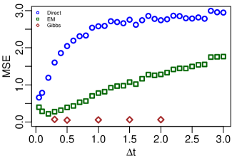
for different time discretization $\Delta t$. For each time step, we generated $20$ data sets, each of size $n=4000$, and computed the MSE on a test set of size $n=2000$ for each data set for both algorithms with RBF kernel. As benchmark reference, we include the estimation results of a Monte Carlo sampler (see appendix C). The latter one is represented only for one data set at small and medium time intervals, respectively, due to its long computation time. In order to improve comparability, we fixed the length scale of the RBF kernel to $l=0.62$ for all data sets.

The results are given in figure 10. The MSE of the direct GP grows quite rapidly for smaller intervals until it reaches an upper bound roughly equivalent with randomly guessing the drift function. On the other hand, the MSE for the EM algorithm increases at a much slower rate, giving good results even for data sets with bigger time distances. The estimation results for the Gibbs sampler are independent of the discretization rate, but take considerable time to compute: while the EM algorithm runs for a couple of minutes, the sampler takes up to two days.

Figure 10: (color online) Comparison of the MSE for different methods over different time intervals.

Double well model with known state dependent diffusion

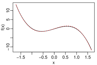
As our next example we examine the double well model with state dependent diffusion and larger time discretization. Here we assume that the diffusion function $D(x)$ is known. Specifically, we sample $n=4000$ observation at $\Delta t=0.5$ and run the EM algorithm with a polynomial kernel of order $p=4$. The direct GP and the EM result are given in figure 9 and 11, respectively. One can clearly see, that an application of the EM algorithm leads to a significantly better estimator of the drift function, compared to the direct GP method.

Figure 11: (color online) GP estimation after one iteration of the EM algorithm. Again, the solid black and red dashed lines denote estimator and true drift function, respectively.

Two dimensional synthetic model

We now turn to a two dimensional process with the following dynamics:

$$dX = (X(1-X^{2}-Y^{2})-Y)dt+dW_{t}^{(1)},$$ (70)

$$dY = (Y(1-X^{2}-Y^{2})+Ý)dt+dW_{t}^{(2)},$$ (71)

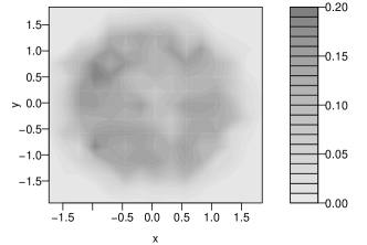
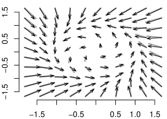
where the component indices are denoted by superscripts. For this model we generated $n=10000$ observations with step size $\Delta t=0.2$ shown in figure 12. The estimation in figure 13 uses a polynomial kernel of order $p=4$ and shows a good fit to the true drift especially in the regions where the observations are concentrated. Note that this is a non-equilibrium model, where the drift cannot be expressed as the gradient of a potential. Hence, the density based method of Batz:2016:VED cannot be applied here.

Figure 12: Empirical density of the two dimensional synthetic model data.

Figure 13: Vector fields of the true drift depicted as grey lines and the estimated drift as black arrows for the two dimensional synthetic data.

Lorenz’63 model

We next analyze a stochastic version of the three dimensional Lorenz’63 model. It consists of the following system of nonlinear coupled stochastic differential equations:

$$dX = \sigma(Y-X)dt+dW_{t}^{(1)},$$ (72)

$$dY = (\rho X-X-XZ)dt+dW_{t}^{(2)},$$ (73)

$$dZ = (XY-\beta Z)dt+dW_{t}^{(3)}.$$ (74)

Lorenz’63 is a chaotic system which was developed as a simplified model of thermal convection in the atmosphere Lorenz:1963:DNF . The parameters $\boldsymbol{\theta}=(\sigma,\rho,\beta)$ are set to the commonly used $\boldsymbol{\theta}=(10,28,8/3)$ known to induce chaotic behavior in the system. In order to analyze the model we simulate $n=3000$ data points with time discretization $\Delta t=0.2$. In the inference, we used a polynomial kernel of order $p=2$ and assume that the constant diffusion is known.

Figure 14: Simulated sample path of the Lorenz’63 model learned by the direct GP algorithm.

Figure 15: Simulated sample path of the Lorenz’63 model learned by the EM algorithm.

Figure 16: Simulated path in the X-Z plane from the Lorenz’63 model learned by the direct GP algorithm.

Figure 17: Simulated path in the X-Z plane from the Lorenz’63 model learned by the EM algorithm.

In order to visualize the quality of the estimation results, we computed the direct GP and the EM algorithm and simulated paths using the corresponding mean estimator as drift function. Here, the application of the EM leads to a vastly superior estimation result compared to the direct method. As shown in figure 16, the direct GP estimator path collapses to a small region of the function space, whereas the EM trajectory of figure 17 nicely captures the true dynamics of the Lorenz’63 model, faithfully recreating the famous butterfly pattern in the X-Z plane.

Cart and pole model

Next, we consider an example from the class of mechanical systems. Our model describes the dynamics of a pole attached to a cart moving randomly along an one-dimensional axis. Formally, we get a system of two dimensional differential equations with $x$ denoting the angle of the pendulum, and $v$ the angular velocity. We define the upright position of the pendulum as $X=0$. This particular cart and pole model is frequently studied in the context of learning control policies Deisenroth:2009:GPD , where the goal is to move the cart in such a way as to stabilize the pendulum in the upright position. The complete system looks as follows:

$$dX = Vdt,$$ (75)

$$dV = \frac{-\gamma V+mgl\sin(X)}{ml^{2}}dt+d^{1/2}dW_{t},$$ (76)

where $\gamma=0.05$ is the friction coefficient, $l=1\mathrm{m}$ and $m=1\mathrm{kg}$ are the length and mass of the pendulum, respectively, and $g=9.81\mathrm{m}\,\mathrm{s}^{-2}$ denotes the gravitational constant. For our experiment, we generated $N=4000$ data points $(x,v)$ on a grid with $\Delta t=0.3$ and known diffusion constant $d=1$. Here, the full diffusion matrix

$$D=\left(\begin{array}[]{cc}0&0\\ 0&1\end{array}\right),$$ (77)

for both $X$ and $V$ is rank deficient due to its noiseless first equation. However, we note that our EM algorithm is also applicable to models with deterministic components, since the E-Step in the EM algorithm remains well defined. In the kernel function we incorporate our prior knowledge that the pendulum angle is periodic and the velocity acts as a linear friction term inside the system. Specifically we define the following multiplicative kernel for the $dV$ equation:

$$K\left((x,v),(x^{\prime},v^{\prime})\right)=K_{\mathrm{Per}}(x,x^{\prime})K_{\mathrm{Poly}}(v,v^{\prime}),$$ (78)

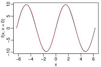
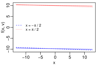
where $K_{\mathrm{Per}}$ denotes the periodic kernel over the state $x$ with hyperparameters $l=1.21$ and $K_{\mathrm{Poly}}$ the polynomial kernel of order $p=1$ over the velocity $V$. The multiplicative kernel structure allows for interactions between its components. Since in this model the components are independent, we could also use an additive kernel, which neglects interactions terms, but we have chosen the more generally applicable variant here. For the $dX$ equation, we use a polynomial kernel of order $p=1$, which captures the linear relationship between $X$ and $V$. If we adapt our choice of the kernel to the specific form of the system, we get an accurate estimate even for data points separated by a wider time spacing (see figures 18 and 19).

Figure 18: (color online) One dimensional drift estimation plots of the second ($dV$) SDE of the cart and pole model. The figure shows the estimation of the pendulum position $X$ for a fixed velocity $V=0$. The solid black line is the drift estimation and the red dashed line the true function.

Figure 19: (color online) One dimensional drift estimation plots of the second ($dV$) SDE of the cart and pole model: Estimation of $V$ for a fixed pendulum position in the horizontal positions with the top pointing to the left $X=-\pi/2$ and to the right side $X=\pi/2$. Full lines denote the drift estimation and dashed and dotted lines the true values.

VI.3 External forces

We can expect a reasonably good estimation of $f(x)$ only in regions of $x$ where we have enough observations. This is of clear importance, when the system is multi-stable and the noise is too small to allow for a sufficient exploration of space. An alternative method for exploration would be to add a known external deterministic control force $u(t)$ to the dynamics which is designed to drive the system from one locally stable region to another one. Hence, we assume an SDE

$$dX_{t}=\left(f(X_{t})+u(t)\right)dt+D^{1/2}dW_{t}.$$ (79)

This situation is easily incorporated into our formalism. In all likelihood terms, we replace $f(X_{t})$ by $f(X_{t})+u(t)$, but keeping the zero mean GP prior over functions. The changes for the corresponding transition probabilities of the approximating time dependent Ornstein-Uhlenbeck bridge are given in appendix B.

We demonstrate the concept by applying it to the double well model. We get

$$dX=(4(X-X^{3})+u(t))dt+\sigma dW_{t}.$$ (80)

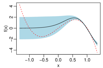
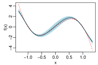
As external force we choose a periodic control function of the form $u(t)=a\sin(\omega t)$ with parameters $a=1$ and $\omega=3$. We generated a data set of $n=2000$ observations on a regular grid with distance $\Delta t=0.2$ from the model with known diffusion $D^{1/2}=0.5$. The addition of $u(t)$ leads to observations from both of the wells, whereas in the uncontrolled case only one part of the underlying state space is explored. Hence, the drift estimation in the latter case leads to an accurate result solely around the well at $X=1$, as opposed to the controlled case, where both modes are truthfully recovered (figures 20 and 21). In both cases, we used a RBF kernel with $\tau=1$. The length scales was set to $l=0.74$ in the controlled and $l=0.53$ in the uncontrolled case.

Figure 20: (color online) EM algorithm predictions for the uncontrolled double well path with the solid black line denoting the estimation and the dashed red line the true drift. Here, the estimation of the well around $X=-1$ basically equals the GP prior, since there are no observations on this region. The shaded area can be interpreted as the 95%-confidence bound.

Figure 21: (color online) EM algorithm predictions for the controlled double well path. The solid black line is the estimated drift and the dashed red line the true function.

VI.4 Diffusion Estimation

As in the dense data scenario, we look at constant and state dependent diffusions in turn. If $D$ does not depend on the state, we can proceed in analogy to the dense data case and maximize the approximate evidence (68) with respect to the diffusion values.

For the state dependent case $D(x)$ we assume a parametric function $D(x;\theta)$, which is specified by its parameter vector $\theta$. Here, we again maximize the likelihood with respect to the corresponding $\theta$.

For an illustration, we don’t show the constant diffusion case and instead restrict ourself to the more interesting case of a state dependent $D(x)$. We sampled $n=8000$ observations at $\Delta t=0.3$ from the following process:

$$dX=0.4(4-X)dt+\max(2-(X-4)^{2},0.25)dW_{t}.$$ (81)

Figure 22: (color online) Comparison of the diffusion estimation for data generated from (81). The dashed red line is the true square root $D(x)^{1/2}$ of the diffusion and the solid black line the parametric estimation based on the EM algorithm. For comparison, we include the estimate based on the direct GP denoted by the green dashed-dotted line.

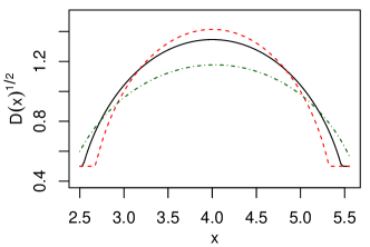
The diffusion function was modelled as $D(x,\mathbf{\theta})=\theta_{1}x^{2}+\theta_{2}x+\theta_{3}$. As kernel function for the drift, we used a polynomial kernel of order $p=1$. Optimizing the evidence with respect to $\bf{\theta}$ leads to the results shown in figure 22. One can see that the estimation gives a reasonably good fit to the true diffusion function even with the bigger time discretization. We note however, that the diffusion estimate is of a lower quality than the drift estimate, since in this case the evidence is less accurate.

VII Discussion

It would be interesting to replace the ad hoc local linear approximation of the posterior drift by a more flexible time dependent Gaussian model. This could be optimized in a variational EM approximation by minimizing a free energy in the E-step, which contains the Kullback-Leibler divergence between the linear and true processes Archambeau:2007:VID ; Vrettas:2015:VMF . Such a method could be extended to noisy observations and the case, where some components of the state vector are not observed. Also, this method could be turned into a variational Bayesian approximation, where one optimizes posteriors over both drifts and over state paths. The path probabilities are then influenced by the uncertainties in the drift estimation, which would lead to more realistic predictions of error bars.

Finally, nonparametric diffusion estimation deserves further attention. Incorporating a fully nonparametric model of the diffusion function $D(x)$ in our scheme would be infeasible in practice, since this would involve the joint estimation of $n$ diffusion matrices. In our experiments, we tried a (quasi-)nonparametric approach, where we represented the diffusion function by its value at a few supporting points and took these as inputs for a GP regression, which we then used as function approximation. However, our experiments have shown that in order to achieve a reasonable estimation quality we need supporting points on a relatively dense grid. The corresponding optimization over the vector of grid points turned out to be too inefficient, which makes the approach impractical. Furthermore, the evidence over which we optimize is often too inaccurate to lead to a reasonable quality.

If performance time is not at all critical, one can resort to a Markov Chain Monte Carlo (MCMC) algorithm, which generates exact samples from the corresponding drift and diffusion functions. In contrast to the EM algorithm, the sampler evaluates the diffusion function on a dense grid and also does not use the assumption of constant diffusion between adjacent observations, thereby overcoming the significant estimation errors for larger time distances. We plan to report on this in a future publication.

Acknowledgments

This work was supported by the European Community’s Seventh Framework Programme (FP7, 2007-2013) under the grant agreement 270327 (CompLACS).

Appendix A Conditional drift

Here, we give the derivation of the conditional drift term $g_{t}(x)$, which occurs in the E-step of the EM algorithm.

$$g_{t}(x) = \lim_{\Delta t\to 0}\frac{1}{\Delta t}\mathrm{E}\left[X_{t+\Delta t}-X_{t}|X_{t}=x,X_{\tau}=y\right]$$

$$= \lim_{\Delta t\to 0}\frac{1}{\Delta t}\frac{\int(x^{\prime}-x)\;p_{\tau-t-\Delta t}(y|x^{\prime})p_{\Delta t}(x^{\prime}|x)\;dx^{\prime}}{\int p_{\tau-t-\Delta t}(y|x^{\prime})p_{\Delta t}(x^{\prime}|x)\;dx^{\prime}}$$

$$= \lim_{\Delta t\to 0}\frac{1}{\Delta t}\frac{f(x)\Delta t+\mathrm{E}_{u}\left[p_{\tau-t-\Delta t}(y|x+f(x)\Delta t+u)u\right]}{\mathrm{E}_{u}\left[p_{\tau-t-\Delta t}(y|x+f(x)\Delta t+u)\right]}$$

$$= f(x)+D\lim_{\Delta t\to 0}\frac{\nabla_{x}\mathrm{E}_{u}\left[p_{\tau-t-\Delta t}(y|x+f(x)\Delta t+u)\right]}{\mathrm{E}_{u}\left[p_{\tau-t-\Delta t}(y|x+f(x)\Delta t+u)\right]}$$

$$= f(x)+D\lim_{\Delta t\to 0}\nabla_{x}\ln\left\{\mathrm{E}_{u}\left[p_{\tau-t-\Delta t}(y|x+f(x)\Delta t+u)\right]\right\}$$

$$= f(x)+D\nabla_{x}\ln\left\{p_{\tau-t}(y|x)\right\}.$$

The second line follows from the definition of the conditional density, the 3rd line from the fact that $p_{\Delta t}(x^{\prime}|x)={\cal{N}}(x+f(x)\Delta t;D\Delta t)$ and $u\sim{\cal{N}}(0;\sigma^{2}\Delta t)$. The fourth line is based on the fact that for zero mean Gaussian random vectors with covariance $S$, we have $\mathrm{E}[ug(u)]=S\mathrm{E}[\nabla_{u}g(u)]$. Finally, the last line is obtained by noting that the covariance of $u$ vanishes for $\Delta t\to 0$.

Appendix B Ornstein-Uhlenbeck bridge with external forces

If there is an additional time-dependent and known drift term $u(t)$, e.g. a control force, in the Ornstein-Uhlenbeck model, i.e.

$$dX_{t}=[f(y_{k})-\Gamma_{k}(X_{t}-y_{k})+u(t)]dt+D_{k}^{1/2}dW,$$

with $\quad\Gamma_{k}=-\nabla f(y_{k})$ and $D_{k}=D(y_{k})$, the mean of the marginal posterior is changed to

$$m(t) =C(t)e^{-\Gamma_{k}^{\top}(\tau-u)}S_{\tau-u}^{-1}\left(x_{k+1}-\alpha_{k}+e^{-\Gamma_{k}(\tau-u)}\alpha_{k}-\int_{u}^{\tau}e^{-\Gamma_{k}(\tau-v)}u(t-u+v)dv\right)$$

$$+C(t)S_{u}^{-1}\left(\alpha_{k}+e^{-\Gamma_{k}u}(x_{k}-\alpha_{k})+\int_{0}^{u}e^{-\Gamma_{k}(u-v)}u(t-u+v))dv\right),$$

but the covariance matrix stays the same. For the posterior drift, we get in this case

$$g_{t}(x)\approx f(x_{k})-\Gamma_{k}(x-x_{k})+D_{k}e^{-\Gamma_{k}^{\top}(\tau-u)}S_{\tau-u}^{-1}\left(x_{k+1}-\alpha_{k}-e^{-\Gamma_{k}(\tau-u)}(x-\alpha_{k})-\int_{u}^{\tau}e^{-\Gamma_{k}(\tau-v)}u(t-u+v))dv\right).$$

For $u(t)=a\sin(\omega t)$:

$$m(t) =C(t)e^{-\gamma_{k}(t_{k+1}-t)}S_{t_{k+1}-t}^{-1}\Big{[}x_{k+1}-\alpha_{k}+e^{-\gamma_{k}(t_{k+1}-t)}\alpha_{k}-\frac{a}{\gamma_{k}^{2}+\omega^{2}}\Big{(}(\gamma_{k}\sin(\omega t_{k+1})-\omega\cos(\omega t_{k+1}))$$

$$-e^{-\gamma_{k}(t_{k+1}-t)}(\gamma_{k}\sin(\omega t)-\omega\cos(\omega t))\Big{)}\Big{]}+C(t)S_{t-t_{k}}^{-1}\Big{[}\alpha_{k}+e^{-\gamma_{k}(t-t_{k})}(x_{k}-\alpha_{k})$$

$$+\frac{a}{\gamma_{k}^{2}+\omega^{2}}\Big{(}(\gamma_{k}\sin(\omega t)-\omega\cos(\omega t))-e^{-\gamma_{k}(t-t_{k})}(\gamma_{k}\sin(\omega t_{k})-\omega\cos(\omega t_{k}))\Big{)}\Big{]},$$

$$g_{t}(x) \approx f(x_{k})+a\sin(\omega t)-\gamma_{k}(x-x_{k})+De^{-\gamma_{k}(t_{k+1}-t)}S_{t_{k+1}-t}^{-1}\Big{[}x_{k+1}-\alpha_{k}-e^{-\gamma_{k}(t_{k+1}-t)}(x-\alpha_{k})$$

$$-\frac{a}{\gamma_{k}^{2}+\omega^{2}}\Big{(}(\gamma_{k}\sin(\omega t_{k+1})-\omega\cos(\omega t_{k+1}))-e^{-\gamma_{k}(t_{k+1}-t)}(\gamma_{k}\sin(\omega t)-\omega\cos(\omega t))\Big{)}\Big{]}.$$

Appendix C MCMC sampler

We briefly describe the Markov Chain Monte Carlo (MCMC) algorithm, which generates samples from the drift function of a system of SDEs with known diffusion. Similar to the EM algorithm in the main text, the drift is modeled in a nonparametric way.

As before, our data will be a set of $N$ observations $\mathbf{Y}=(y_{1},\ldots,y_{N})$, where $y_{k}=X_{k\tau}$. Since the time distance between adjacent observations is taken to be large, we impute the process between observations in interval $I_{k}=[k\,\tau;(k+1)\tau]$ on a fine grid of step size $\Delta=\tau/M$ for some suitable integer $M$. The imputed path of the $k$th subinterval will be denoted by $\mathbf{X}_{k}=\left\{X_{k\tau},X_{k\tau+\Delta},\ldots,X_{k\tau+M\Delta}\right\}$.

If we write the complete imputed path of length $MN$ as

$$\mathbf{X}=(y_{0},X_{\Delta},\ldots,X_{(M-1)\Delta},\ldots,y_{1},\ldots,\\ X_{(k-1)\tau+(M-1)\Delta},y_{k},X_{k\tau+\Delta},\ldots,y_{N}),$$

then the joint posterior distribution of the data and the drift and diffusion function for a given set of observations is given by

$$p(\mathbf{X},f|\mathbf{Y},D)\propto p_{0}(f)\prod_{l=1}^{NM}p(X^{l+1}|X^{l},f,D)$$

Here, the density $p(\mathbf{X},f|\mathbf{Y},D)$ is approximately normally distributed(see (5)) on the fine grid with mean and variance given by (20) and (21), respectively. A straightforward way to sample from this posterior is given by the following Gibbs sampler:

Algorithm 1 Gibbs Sampler

1:Initialize $f^{(0)}$ with the direct GP solution

2:for $i=1,\ldots,N$ do

3:     Sample $\mathbf{X}^{(i)}\sim p(\mathbf{X}|\mathbf{Y},f^{(i-1)},D)$

4:     Sample $f^{(i)}\sim p(f|\mathbf{X}^{(i)},\mathbf{Y})$

Here, the superscripts denote the iteration. The number of iterations for a particular model is determined by the usual MCMC convergence diagnostics, see for example Robert:2013:MSM . Since an analytic form for the imputed path distribution $p(\mathbf{X}|\mathbf{Y},f,D)$ does not exist, we have to resort to a Metropolis- Hasting (MH) step. As proposal distribution $q$, we use the so-called modified diffusion bridge (MBD) of Durham:2002:NTM . Here, for each interval $I_{k}$ the density of a grid point $X_{k}^{j+1}$ from $\mathbf{X}_{k}$ is normally distributed, conditioned on $X_{k}^{j}$ and the interval endpoint $y_{k+1}$:

$$q(X_{k}^{j+1}|X_{k}^{j},y_{k+1},f_{q},D_{q})=\\ \mathcal{N}(X_{k}^{j+1}|X_{k}^{j}+f_{q}(X_{k}^{j})\Delta,D_{q}(X_{k}^{j}))$$ (82)

with drift and diffusion

$$f_{q}(X_{k}^{j})=\frac{y_{k+1}-X^{j}}{\tau-j\Delta},\quad D_{q}(X_{k}^{j})=\frac{\tau-(j+1)\Delta}{\tau-j\Delta}D(X_{k}^{j}).$$

Now, since for each subinterval $I_{k}$ the bridge proposal starts in observation $y_{k}$ and terminates in $y_{k+1}$, we can generate a sample of the complete path $p(\mathbf{X}|\mathbf{Y},f,D)$ by sampling a MDB proposal separately for each the $N$ subintervals. Specifically, for subinterval $I_{k}$ we simulate a path $\mathbf{X}^{*}_{k}$ on the dense grid by recursively sampling from (82) and move from current state $\mathbf{X}_{k}$ to $\mathbf{X}^{*}_{k}$ with probability

$$\alpha(\mathbf{X}_{k},\mathbf{X}^{*}_{k})=\min\left\{1,\left[\prod_{j=1}^{M-1}\frac{p(X_{k}^{*(j+1)}|X_{k}^{*j},f,D)}{p(X_{k}^{j+1}|X_{k}^{j},f,D)}\right]\right.\\ \left.\times\left[\prod_{j=1}^{M-2}\frac{q(X_{k}^{j+1}|X_{k}^{j},y_{k+1},f_{q},D_{q})}{q(X_{k}^{*(j+1)}|X_{k}^{*j},y_{k+1},f_{q},D_{q})}\right]\right\},$$

with probability $(1-\alpha(\mathbf{X}_{k},\mathbf{X}^{*}_{k}))$ we retain the current path $\mathbf{X}_{k}$.

The sampling from the drift $p(f|\mathbf{X},\mathbf{Y})$ is easier to accomplish, since under a GP prior $p_{0}\sim\mathcal{GP}$ assumption, the distribution $p(f|\mathbf{Y},\mathbf{X})$ of the SDE drift corresponds to a GP posterior and is therefore of analytic form. Since the number of dense path observations is usually quite substantial, we resort to the sparse version of the GP with mean and variance given by (45) and (46), respectively. In each iteration of the Gibbs sampler, we simulate a new $f$ on a fine grid over the (slightly extended) range of the path observations $\mathbf{X}$ and then interpolate these points by nonparametric regression in order to arrive at an approximate drift function. The interpolation step, for which we again resort to a sparse GP, is motivated by computational considerations, since this way evaluating the function values for the path can be can be done very efficiently, while also being accurate due to the smoothness of the underlying drift.

References

- [1] C. W. Gardiner. Handbook of Stochastic Methods. Springer, Berlin, second edition, 1996.
- [2] Stefano M. Iacus. Simulation and Inference for Stochastic Differential Equations: With R Examples (Springer Series in Statistics). Springer, 1st edition, 2008.
- [3] Hao Wu and Frank Noe. Bayesian framework for modeling diffusion processes with nonlinear drift based on nonlinear and incomplete observations. Phys. Rev. E, 83(3):036705, 2011.
- [4] Andrew Golightly and Darren J Wilkinson. Markov chain monte carlo algorithms for sde parameter estimation. Learning and Inference for Computational Systems Biology, pages 253–276, 2010.
- [5] Steven J. Lade. Finite sampling interval effects in kramers–moyal analysis. Phys. Lett. A, 373(41):3705–3709, 2009.
- [6] Federico M. Bandi and Peter C. B. Phillips. Fully nonparametric estimation of scalar diffusion models. Econometrica, 71(1):241–283, 2003.
- [7] Omiros Papaspiliopoulos, Yvo Pokern, Gareth O. Roberts, and Andrew M. Stuart. Nonparametric estimation of diffusions: a differential equations approach. Biometrika, 99(3):511–531, 2012.
- [8] Yvo Pokern, Andrew M. Stuart, and J.H. van Zanten. Posterior consistency via precision operators for Bayesian nonparametric drift estimation in SDEs. Stochastic Processes and their Applications, 123(2):603–628, 2013.
- [9] Frank van der Meulen, Moritz Schauer, and Harry van Zanten. Reversible jump mcmc for nonparametric drift estimation for diffusion processes. Computational Statistics & Data Analysis, 71:615–632, 2014.
- [10] Philipp Batz, Andreas Ruttor, and Manfred Opper. Variational estimation of the drift for stochastic differential equations from the empirical density. Journal of Statistical Mechanics: Theory and Experiment, (8):083404, 2016.
- [11] Arthur P Dempster, Nan M Laird, and Donald B Rubin. Maximum likelihood from incomplete data via the em algorithm. Journal of the royal statistical society. Series B (methodological), pages 1–38, 1977.
- [12] Andreas Ruttor, Philipp Batz, and Manfred Opper. Approximate gaussian process inference for the drift function in stochastic differential equations. In Advances in Neural Information Processing Systems, pages 2040–2048, 2013.
- [13] P. E. Kloeden and E. Platen. Numerical Solution of Stochastic Differential Equations. Springer, New York, corrected edition, June 2011.
- [14] C. E. Rasmussen and C. K. I. Williams. Gaussian Processes for Machine Learning. MIT Press, 2006.
- [15] Cédric Archambeau, Manfred Opper, Yuan Shen, Dan Cornford, and John Shawe-Taylor. Variational inference for diffusion processes. In J.C. Platt, D. Koller, Y. Singer, and S. Roweis, editors, Advances in Neural Information Processing Systems 20, pages 17–24. MIT Press, Cambridge, MA, 2008.
- [16] Katrine K Andersen, N Azuma, J-M Barnola, Matthias Bigler, P Biscaye, N Caillon, J Chappellaz, Henrik Brink Clausen, Dorthe Dahl-Jensen, Hubertus Fischer, et al. High-resolution record of northern hemisphere climate extending into the last interglacial period. Nature, 431(7005):147–151, 2004.
- [17] Frank Kwasniok. Analysis and modelling of glacial climate transitions using simple dynamical systems. Philosophical Transactions of the Royal Society A: Mathematical, Physical and Engineering Sciences, 371(1991), 2013.
- [18] Michalis K. Titsias. Variational learning of inducing variables in sparse Gaussian processes. JMLR WC&P, 5:567–574, 2009.
- [19] Lehel Csató, Manfred Opper, and Ole Winther. TAP Gibbs free energy, belief propagation and sparsity. In T. G. Dietterich, S. Becker, and Z. Ghahramani, editors, Advances in Neural Information Processing Systems 14, pages 657–663. MIT Press, 2002.
- [20] Athanasios Papoulis. Probability, random variables, and stochastic processes. 1965.
- [21] Lehel Csató and Manfred Opper. Sparse on-line gaussian processes. Neural Computation, 14(3):641–668, 2002.
- [22] H.A. Sturges. The choice of a class interval. Journal of the American Statistical Association, 21:65–66, 1926.
- [23] Edward N Lorenz. Deterministic nonperiodic flow. Journal of the atmospheric sciences, 20(2):130–141, 1963.
- [24] Marc Peter Deisenroth, Carl Edward Rasmussen, and Jan Peters. Gaussian process dynamic programming. Neurocomputing, 72(7):1508–1524, 2009.
- [25] Michail D. Vrettas, Dan Cornford, and Manfred Opper. Variational mean-field algorithm for efficient inference in large systems of stochastic differential equations. Phys. Rev. E, 91:012148, 2015.
- [26] Christian Robert and George Casella. Monte Carlo statistical methods. Springer Science & Business Media, 2013.
- [27] Garland B Durham and A Ronald Gallant. Numerical techniques for maximum likelihood estimation of continuous-time diffusion processes. Journal of Business & Economic Statistics, 20(3):297–338, 2002.