Algorithms for Online Influencer Marketing

Abstract

Influence maximization is the problem of finding influential users, or nodes, in a graph so as to maximize the spread of information. It has many applications in advertising and marketing on social networks. In this paper, we study a highly generic version of influence maximization, one of optimizing influence campaigns by sequentially selecting “spread seeds” from a set of influencers, a small subset of the node population, under the hypothesis that, in a given campaign, previously activated nodes remain “persistently” active throughout and thus do not yield further rewards. This problem is in particular relevant for an important form of online marketing, known as influencer marketing, in which the marketers target a sub-population of influential people, instead of the entire base of potential buyers. Importantly, we make no assumptions on the underlying diffusion model and we work in a setting where neither a diffusion network nor historical activation data are available. We call this problem online influencer marketing with persistence (in short, OIMP). We first discuss motivating scenarios and present our general approach. We introduce an estimator on the influencers’ remaining potential – the expected number of nodes that can still be reached from a given influencer – and justify its strength to rapidly estimate the desired value, relying on real data gathered from Twitter. We then describe a novel algorithm, GT-UCB, relying on upper confidence bounds on the remaining potential. We show that our approach leads to high-quality spreads on both simulated and real datasets, even though it makes almost no assumptions on the diffusion medium. Importantly, it is orders of magnitude faster than state-of-the-art influence maximization methods, making it possible to deal with large-scale online scenarios.

Keywords:Influencer marketing, information diffusion, online social networks, influence maximization, online learning, multi-armed bandits.

1 Introduction

Advertising based on word-of-mouth diffusion in social media has become very important in the digital marketing landscape. Nowadays, social value and social influence are arguably the hottest concepts in the area of Web advertising and most companies that advertise in the Web space must have a “social” strategy. For example, on widely used platforms such as Facebook or Twitter, promoted posts are interleaved with normal posts on user feeds. Users interact with these posts by actions such as “likes” (adoption), “shares” or “reposts” (network diffusion). This represents an unprecedented utility in advertising, be it with a commercial intent or not, as products, news, ideas, movies, political manifests, tweets, etc, can propagate easily to a large audience [40, 41].

Motivated by the need for effective viral marketing strategies, influence estimation and influence maximization have become important research problems, at the intersection of data mining and social sciences [12]. In short, influence maximization is the problem of selecting a set of nodes from a given diffusion graph, maximizing the expected spread under an underlying diffusion model. This problem was introduced in $2003$ by the seminal work of Kempe et al. [21], through two stochastic, discrete-time diffusion models, Linear Threshold (LT) and Independent Cascade (IC). These models rely on diffusion graphs whose edges are weighted by a score of influence. They show that selecting the set of nodes maximizing the expected spread is NP-hard for both models, and they propose a greedy algorithm that takes advantage of the sub-modularity property of the influence spread, but does not scale to large graphs. A rich literature followed, focusing on computationally efficient and scalable algorithms to solve influence maximization. The recent benchmarking study of Arora et al. [2] summarizes state-of-the-art techniques and also debunks many influence maximization myths. In particular, it shows that, depending on the underlying diffusion model and the choice of parameters, each algorithm’s behavior can vary significantly, from very efficient to prohibitively slow, and that influence maximization at the scale of real applications remains an elusive target.

Importantly, all the influence maximization studies discussed in [2] have as starting point a specific diffusion model (IC or LT), whose graph topology and parameters – basically the edge weights – are known. In order to infer the diffusion parameters or the underlying graph structure, or both, [15, 16, 14, 18, 33, 11] propose offline, model-specific methods, which rely on observed information cascades. In short, information cascades are time-ordered sequences of records indicating when a specific user was activated or adopted a specific item.

There are however many situations where it is unreasonable to assume the existence of relevant historical data in the form of cascades. For such settings, online approaches, which can learn the underlying diffusion parameters while running diffusion campaigns, have been proposed. Bridging influence maximization and inference, this is done by balancing between exploration steps (of yet uncertain model aspects) and exploitation ones (of the best solution so far), by so called multi-armed bandits techniques, where an agent interacts with the network to infer influence probabilities [38, 10, 42, 37]. The learning agent sequentially selects seeds from which diffusion processes are initiated in the network; the obtained feedback is used to update the agent’s knowledge of the model.

Nevertheless, all these studies on inferring diffusion networks, whether offline or online, rely on parametric diffusion models, i.e., assume that the actual diffusion dynamics are well captured by such a model (e.g., IC). This maintains significant limitations for practical purposes. First, the more complex the model, the harder to learn in large networks, especially in campaigns that have a relatively short timespan, making model inference and parameter estimation very challenging within a small horizon (typically tens or hundreds of spreads). Second, it is commonly agreed that the aforementioned diffusion models represent elegant yet coarse interpretations of a reality that is much more complex and often hard to observe fully. For examples of insights into this complex reality, the topical or non-topical nature of an influence campaign, the popularity of the piece of information being diffused, or its specific topic were all shown to have a significant impact on hashtag diffusions in Twitter [11, 19, 32].

Our contribution

Aiming to address such limitations, we propose in this paper a large-scale approach for online and adaptive influence maximization, in which the underlying assumptions for the diffusion processes are kept to a minimum (if, in fact, hardly any).

We argue that it can represent a versatile tool in many practical scenarios, including in particular the one of influencer marketing, which, according to Wikipedia, can be described as follows: “a form of marketing in which focus is placed on influential people rather than the target market as a whole, identifying the individuals that have influence over potential buyers, and orienting marketing activities around these influencers”. For instance, influential users may be contractually bound by a sponsorship, in exchange for the publication of promoted posts on their online Facebook or Twitter accounts. This new form of marketing is by now extensively used in online social platforms, as is discussed in the marketing literature [13, 1, 6].

More concretely, we focus on social media diffusion scenarios in which influence campaigns consist of multiple consecutive trials (or rounds) spreading the same type of information from an arbitrary domain (be it a product, idea, post, hashtag, etc). The goal of each campaign is to reach (or activate) as many distinct users as possible, the objective function being the total spread. These potential influencees – the target market – represent the nodes of an unknown diffusion medium / online network. In our setting – as, arguably, in many real-world scenarios – the campaign selects from a known set of spread seed candidates, so called influencers, a small subset of the potentially large and unknown target market. At each round, the learning agent picks among the influencers those from which a new diffusion process is initiated in the network, gathers some feedback on the activations, and adapts the subsequent steps of the campaign. Only the effects of the diffusion process, namely the activations (e.g., purchases or subscriptions), are observed, but not the process itself. The agent may “re-seed” certain influencers (we may want to ask a particular one to initiate spreads several times, e.g., if it has a strong converting impact). This perspective on influence campaigns imposes naturally a certain notion of persistence, which is given the following interpretation: users that were already activated in the ongoing campaign – e.g., have adopted a product or endorsed a political movement – remain activated throughout that campaign, and thus will not be accounted for more than once in the objective function.

We call this problem online influencer marketing with persistence (in short, OIMP). Our solution for it follows the multi-armed bandit idea initially employed in Lei et al. [24], but we adopt instead a diffusion-independent perspective, whose only input are the spread seed candidates, while the population and underlying diffusion network – which may actually be the superposition of several networks – remain unknown. In our bandit approach, the parameters to be estimated are the values of the influencers – how good is a specific influencer –, as opposed to the diffusion edge probabilities of a known graph as in [24]. Furthermore, we make the model’s feedback more realistic by assuming that after each trial, the agent only gathers the set of activated nodes. The rationale is that oftentimes, for a given “viral” item, we can track in applications only when it was adopted by various users, but not why. A key difference w.r.t. other multi-armed bandit studies for influence maximization such as [38, 10, 42, 37] is that these look for a constant optimal set of seeds, while the difficulty with OIMP is that the seemingly best action at a given trial depends on the activations of the previous trials (and thus the learning agent’s past decisions).

The multi-armed bandit algorithm we propose, called GT-UCB, relies on a famous statistical tool known as the Good-Turing estimator, first developed during WWII to crack the Enigma machine, and later published by Good in a study on species discovery [17]. Our approach is inspired by the work of Bubeck et al. [8], which proposed the use of the Good-Turing estimator in a context where the learning agent needs to sequentially select experts that only sample one of their potential nodes at each trial. In contrast, in OIMP, when an influencer is selected, it may have a potentially large spread and may activate many nodes at once. Our solution follows the well-known optimism in the face of uncertainty principle from the bandit literature (see [7] for an introduction to multi-armed bandit problems), by deriving an upper confidence bound on the estimator for the remaining potential for spreading information of each influencer, and by choosing in a principled manner between explore and exploit steps.

In Section 6 we evaluate the proposed approach on publicly available graph datasets as well a large snapshot of Twitter activity we collected. The proposed algorithm is agnostic with respect to the choice of influencers, who in most realistic applications will be selected based on a combination of graph-based and external considerations. We describe however in Section 6.1 several heuristics that may be used to automatically extract good candidates for the influencer set, when a social network graph is available. This choice of influencers also makes it possible to compare the results obtained by our method to those of the baseline methods from the literature (see above), which require knowledge of the graph and of the diffusion model and, in some cases, of the influence probabilities.

Comparison with previous publication

We extend in this article a preliminary study published in Lagrée et al. [22], introducing the following new contributions, which allow us to give a complete picture on our model and algorithmic solutions:

• A more detailed discussion on the motivation behind our work, in relation to new forms of online marketing, such as influencer marketing.

• An empirical analysis over Twitter data, which comes to support the assumptions behind our choice of estimators for the remaining potential in each influencer.

• A detailed theoretical analysis and justification for the upper confidence bounds on which our algorithm GT-UCB relies.

• Theoretical guarantees on the performance of GT-UCB, formulated in terms of waiting time, a notion that is better suited in our bandit framework than the usual one of regret.

• An adaptation of GT-UCB (denoted Fat-GT-UCB) and the corresponding theoretical analysis, for scenarios in which influencers may experience fatigue, i.e., a diminishing tendency to activate their user base as they are re-seeded throughout a marketing campaign.

• A broader experimental analysis involving the two datasets previously used in [22], as well as a new set of experimental results in a completely different scenario, involving real influence spreads from Twitter, for both GT-UCB and Fat-GT-UCB.

To the best of our knowledge, our approach is the first to show that efficient and effective influence maximization can be done in a highly uncertain or under-specified social environment, along with formal guarantees on the achieved spread.

2 Setting

The goal of the online influencer marketing with persistence is to successively select (or activate) a number of seed nodes, in order to reach (or spread to) as many other nodes as possible. In this section, we formally define this problem.

2.1 Background

Given a graph $G=(V,E)$, the traditional problem of influence maximization is to select a set of seed nodes $I\subseteq V$, under a cardinality constraint $|I|=L$, such that the expected spread – that is, the number of activated nodes – of an influence cascade starting from $I$ is maximized. Formally, denoting by the random variable $S(I)$ the spread initiated by the seed set $I$, influence maximization aims to solve the following optimization problem:

$$\operatorname*{arg\,max}_{I\subseteq V,|I|=L}\mathbb{E}[|S(I)|].$$

As mentioned before, a plethora of algorithms have been proposed to solve the influence maximization problem, under specific diffusion models. These algorithms can be viewed as full-information and offline approaches: they choose all the seeds at once, in one step, and they have the complete diffusion configuration, i.e., the graph topology and the influence probabilities.

In the online case, during a sequence of $N$ (called hereafter the budget) consecutive trials, $L$ seed nodes are selected at each trial, and feedback on the achieved spread from these seeds is collected.

2.2 Influence maximization via influencers

The short timespan of campaigns makes parameter estimation very challenging within small horizons. In other cases, the topology – or even the existence – of a graph is too strong an assumption. In contrast to [24], we do not try to estimate edge probabilities in some graph, but, instead, we assume the existence of a known set of spread seed candidates – in the following referred to as the influencers – who are the only access to the medium of diffusion. Formally, we let $[K]:=\{1,\ldots,K\}$ be a set of influencers up for selection; each influencer is connected to an unknown and potentially large base (the influencer’s support) of basic nodes, each with an unknown activation probability. For illustration, we give in Figure 1 an example of this setting, with $3$ influencers connected to $4$, $5$, and $4$ basic nodes, respectively.

Now, the problem boils down to estimating the value of the $K$ influencers, which is typically much smaller than the number of parameters of the diffusion model. The medium over which diffusion operates may be a diffusion graph but we make no assumption on that, meaning that the diffusion may also happen in a completely unknown environment. Finally, note that by choosing $K=|V|$ influencers, the classic influence maximization problem can be seen as a special instance of our setting.

Figure 1: Three influencers with associated activation probabilities $p_{k}(u)$.

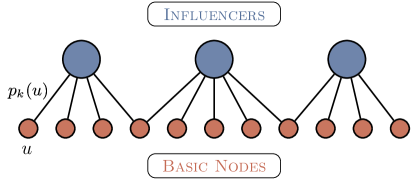
We complete the formal setting by assuming the existence of $K$ sets $A_{k}\subseteq V$ of basic nodes such that each influencer $k\in[K]$ is connected to each node in $A_{k}$. We denote $p_{k}(u)$ the probability for influencer $k$ to activate the child node $u\in A_{k}$. In this context, the diffusion process can be abstracted as follows.

Definition 1 (Influence process).

When an influencer $k\in[K]$ is selected, each basic node $u\in A_{k}$ is sampled for activation, according to its probability $p_{k}(u)$. The feedback for $k$’s selection consists of all the activated nodes, while the associated reward consists only of the newly activated ones.

Remark

Limiting the influence maximization method to working with a small subset of the node base may allow to accurately estimate their value more rapidly, even in a highly uncertain environment, hence the algorithmic interest. At the same time, this is directly motivated by marketing scenarios involving marketers who may not have knowledge of the entire diffusion graph, only having access to a few influential people who can diffuse information (the influencers in our setting), or may simply prefer such a two-step flow of diffusion for various reasons, such as establishing credibility. Moreover, despite the fact that we model the social reach of every influencer by 1-hop links to the to-be-influenced nodes, these edges are just an abstraction of the activation probability, and may represent in reality longer paths in an underlying unknown real influence graph $G$.

2.3 Online influencer marketing with persistence

We are now ready to define the online influencer marketing with persistence task.

Problem 1 (OIMP).

Given a set of influencers $[K]:=\{1,\ldots,K\}$, a budget of $N$ trials, and a number $1\leq L\leq K$ of influencers to be activated at each trial, the objective of the online influencer marketing with persistence (OIMP) is to solve the following optimization problem:

$$\operatorname*{arg\,max}_{I_{n}\subseteq[K],|I_{n}|=L,\forall 1\leqslant n\leqslant N}\mathbb{E}\left|\bigcup_{1\leqslant n\leqslant N}S(I_{n})\right|.$$

As noticed in [24], the offline influence maximization can be seen as a special instance of the online one, where the budget is $N=1$. Note that, in contrast to persistence-free online influence maximization – considered, e.g., in [38, 42] – the performance criterion used in OIMP displays the so-called diminishing returns property: the expected number of nodes activated by successive selections of a given seed is decreasing, due to the fact that nodes that have already been activated are discounted. We refer to the expected number of nodes remaining to be activated as the remaining potential of a seed. The diminishing returns property implies that there is no static best set of seeds to be selected, but that the algorithm must follow an adaptive policy, which can detect that the remaining potential of a seed is small and switch to another seed that has been less exploited. Our solution to this problem has to overcome challenges on two fronts: (1) it needs to estimate the potential of nodes at each round, without knowing the diffusion model nor the activation probabilities, and (2) it needs to identify the currently best influencers, according to their estimated potentials.

Other approaches for the online influence maximization problem rely on estimating diffusion parameters [24, 38, 42] – generally, a distribution over the influence probability of each edge in the graph. However, the assumption that one can estimate accurately the diffusion parameters – and notably the diffusion probabilities – may be overly ambitious, especially in cases where the number of allowed trials (the budget) is rather limited. A limited trial setting is arguably more in line with real-world campaigns: take as example political or marketing campaigns, which only last for a few weeks.

In our approach, we work with parameters on nodes, instead of edges. More specifically, these parameters represent the potentials of remaining spreads from each of the influencer nodes. We stress that this potential can evolve as the campaign proceeds. In this way, we can go around the dependencies on specific diffusion models, and furthermore, we can remove entirely the dependency on a detailed graph topology.

3 Algorithm

In this section, we describe our UCB-like algorithm, which relies on the Good-Turing estimator to sequentially select the seeds to activate at each round, from the available influencers.

3.1 Remaining potential and Good-Turing estimator

A good algorithm for OIMP should aim at selecting the influencer $k$ with the largest potential for influencing its children $A_{k}$. However, the true potential value of an influencer is a priori unknown to the decision maker.

In the following, we index trials by $t$ when referring to the time of the algorithm, and we index trials by $n$ when referring to the number of selections of the influencer. For example, the $t$-th spread initiated by the algorithm is noted $S(t)$ whereas the $n$-th spread of influencer $k$ is noted $S_{k,n}$.

Definition 2 (Remaining potential $R_{k}(t)$).

Consider an influencer $k\in[K]$ connected to $A_{k}$ basic nodes. Let $S(1),\ldots,S(t)$ be the set of nodes that were activated during the first $t$ trials by the seeded influencers. The remaining potential $R_{k}(t)$ is the expected number of new nodes that would be activated upon starting the $t+1$-th cascade from $k$:

$$R_{k}(t):=\sum_{u\in A_{k}}\mathds{1}\left\{u\notin\bigcup_{i=1}^{t}S(i)\right\}p_{k}(u),$$

where $\mathds{1}\{\cdot\}$ denotes the indicator function.

Definition 2 provides a formal way to obtain the remaining potential of an influencer $k$ at a given time. The optimal policy would simply select the influencer with the largest remaining potential at each time step. The difficulty is, however, that the probabilities $p_{k}(u)$ are unknown. Hence, we have to design a remaining potential estimator $\hat{R}_{k}(t)$ instead. It is important to stress that the remaining potential is a random quantity, because of the dependency on the spreads $S(1),\dots,S(t)$. Furthermore, due to the diminishing returns property, the sequence $(S_{k,n})_{n\geq 1}$ is stochastically decreasing.

Following ideas from [17, 8], we now introduce a version of the Good-Turing statistic, tailored to our problem of rapidly estimating the remaining potential. Denoting by $n_{k}(t)$ the number of times influencer $k$ has been selected after $t$ trials, we let $S_{k,1},\ldots,S_{k,n_{k}(t)}$ be the $n_{k}(t)$ cascades sampled independently from influencer $k$. We denote by $U_{k}(u,t)$ the binary function whose value is $1$ if node $u$ has been activated exactly once by influencer $k$ – such occurrences are called hapaxes in linguistics – and $Z_{k}(u,t)$ the binary function whose value is $1$ if node $u$ has never been activated by influencer $k$. The idea of the Good-Turing estimator is to estimate the remaining potential as the proportion of hapaxes in the $n_{k}(t)$ sampled cascades, as follows:

$$\hat{R}_{k}(t):=\frac{1}{n_{k}(t)}\sum_{u\in A_{k}}U_{k}(u,t)\prod_{l\neq k}Z_{l}(u,t).$$

Albeit simple, this estimator turns out to be quite effective in practice. If an influencer is connected to a combination of both nodes having high activation probabilities and nodes having low activation probabilities, then successive traces sampled from this influencer will result in multiple activations of the high-probability nodes and few of the low-probability ones. Hence, after observing a few spreads, the influencer’s potential will be low, a fact that will be captured by the low proportion of hapaxes. In contrast, estimators that try to estimate each activation probability independently will require a much larger number of trials to properly estimate the influencer’s potential.

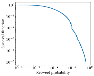
To verify this assumption in reality, we conducted an analysis of the empirical activation probabilities from a Twitter dataset. Specifically, we used a collection of tweets and re-tweets gathered via crawling in August 2012. For each original tweet, we find all corresponding retweets, and, for each user, we compute the empirical probability of a retweet occurring – this, in our case, is a proxy measure for influence probability. Specifically, for every user $v$ “influenced” by $u$, i.e., $v$ retweeted at least one original tweet from $u$ – we compute the estimated diffusion probability: $p_{u,v}=\left|\text{$u$'s tweets retweeted by $v$}\right|/\left|\text{tweets by $u$}\right|$. In Fig. 2 (left), we show the survival function of resulting empirical probabilities in a log-log plot. We can see that most probabilities are small – the 9th decile has value $0.045$.

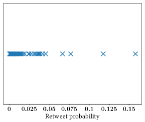
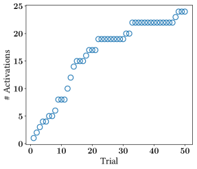
In Fig. 2 (right), we simulated the activation probabilities of a set of $50$ nodes whose activation probabilities are chosen randomly from the Twitter empirical probabilities. Most of the sampled values are low, except a few relatively high ones. Using this sample as the activation probabilities of an hypothetical influencer node, we observe on Fig. 3 (left) the cumulative influence spread. The curve first shows a steep increase until approximately $20$ rounds, where users with high probabilities of conversion have already been activated, while remaining ones are difficult to activate.

Figure 2: (left) Twitter empirical retweet probabilities. (right) Sample of $50$ empirical retweet probabilities.

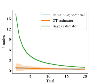
In Fig. 3 (right), we compare the Good-Turing estimator to a Bayesian estimator that maintains a posterior (through a Beta distribution) on the unknown activation probabilities, updating the posterior after each trial, similarly to [24]. In the Bayesian approach, the remaining potential can be estimated by summing over the means of the posterior distributions corresponding to nodes that have not been activated so far. On Fig. 3 (right), the curves are averaged over $200$ runs, and the shaded regions correspond to the $95\%$ quantiles. Clearly, the Good-Turing estimator is much faster than its Bayesian counterpart in estimating the actual remaining potential. Varying the number of nodes – here equal to 50 – shows that the time needed for the Bayesian estimator to provide a reliable estimate of the remaining potential is proportional to the number of nodes, whereas it grows only sub-linearly for the Good-Turing estimator.

Figure 3: (left) Influence spread against number of rounds. (right) Bayesian estimator against Good-Turing estimator.

Remark

While bearing similarities with the traditional missing mass concept, we highlight one fundamental difference between the remaining potential and the traditional missing mass studied in [8], which impacts both the algorithmic solution and the analysis. Since at each step, after selecting an influencer, every node connected to that influencer is sampled, the algorithm receives a larger feedback than in [8], whose feedback is in $[0,1]$. However, on the contrary to [8], the hapaxes of an influencer $(U_{k}(u,t))_{u\in A_{k}}$ are independent. Interestingly, the quantity $\lambda_{k}:=\sum_{u\in A_{k}}p(u)$, which corresponds to the expected number of basic nodes an influencer activates or re-activates in a cascade, will prove to be a crucial ingredient for our problem.

3.2 Upper confidence bounds

Following principles from the bandit literature, the GT-UCB algorithm relies on optimism in the face of uncertainty. At each step (trial) $t$, the algorithm selects the highest upper-confidence bound on the remaining potential – denoted by $b_{k}(t)$ – and activates (plays) the corresponding influencer $k$. This algorithm achieves robustness against the stochastic nature of the cascades, by ensuring that influencers who “underperformed” with respect to their potential in previous trials may still be selected later on. Consequently, GT-UCB aims to maintain a degree of exploration of influencers, in addition to the exploitation of the best influencers as per the feedback gathered so far.

0:  Set of influencers $[K]$, time budget $N$

1:  Initialization: play each influencer $k\in[K]$ once, observe the spread $S_{k,1}$, set $n_{k}=1$

2:  For each $k\in[K]$: update the reward $W=W\cup S_{k,1}$

3:  for $t=K+1,\ldots,N$ do

4:     Compute $b_{k}(t)$ for every influencer $k$

5:     Choose $k(t)=\operatorname*{arg\,max}_{k\in[K]}b_{k}(t)$

6:     Play influencer $k(t)$ and observe spread $S(t)$

7:     Update cumulative reward: $W=W\cup S(t)$

8:     Update statistics of influencer $k(t)$: $n_{k(t)}(t+1)=n_{k(t)}(t)+1$ and $S_{k,n_{k}(t)}=S(t)$.

9:  end for

10:  return  $W$

ALGORITHM 1 – GT-UCB ($L=1$)

Algorithm 1 presents the main components of GT-UCB for the case $L=1$, that is, when a single influencer is chosen at each step.

The algorithm starts by activating each influencer $k\in[K]$ once, in order to initialize its Good-Turing estimator. The main loop of GT-UCB occurs at lines 3-9. Let $S(t)$ be the observed spread at trial $t$, and let $S_{k,s}$ be the result of the $s$-th diffusion initiated at influencer $k$. At every step $t>K$, we recompute for each influencer $k\in[K]$ its index $b_{k}(t)$, representing the upper confidence bound on the expected reward in the next trial. The computation of this index uses the previous samples $S_{k,1},\ldots,S_{k,n_{k}(t)}$ and the number of times each influencer $k$ has been activated up to trial $t$, $n_{k}(t)$. Based on the result of Theorem 1 – whose statement and proof are delayed to Section 4 –, the upper confidence bound is set as:

$$b_{k}(t)=\hat{R}_{k}(t)+\left(1+\sqrt{2}\right)\sqrt{\frac{\hat{\lambda}_{k}(t)\log(4t)}{n_{k}(t)}}+\frac{\log(4t)}{3n_{k}(t)},$$ (1)

where $\hat{R}_{k}(t)$ is the Good-Turing estimator and $\hat{\lambda}_{k}(t):=\sum_{s=1}^{n_{k}(t)}\frac{|S_{k,s}|}{n_{k}(t)}$ is an estimator for the expected spread from influencer $k$.

Then, in line 5, GT-UCB selects the influencer $k(t)$ with the largest index, and initiates a cascade from this node. The feedback $S(t)$ is observed and is used to update the cumulative reward set $W$. We stress again that $S(t)$ provides only the Ids of the nodes that were activated, with no information on how this diffusion happened in the hidden diffusion medium. Finally, the statistics associated to the chosen influencer $k(t)$ are updated.

3.3 Extensions for the case $L>1$

Algorithm 1 can be easily adapted to select $L>1$ influencers at each round. Instead of choosing the influencer maximizing the Good-Turing UCB in line 5, we can select those having the $L$ largest indices. Note that $k(t)$ then becomes a set of $L$ influencers. A diffusion is initiated from the associated nodes and, at termination, all activations are observed. Similarly to [37], the algorithm requires feedback to include the influencer responsible for the activation of each node, in order to update the corresponding statistics accordingly.

4 Analysis

In this section, we justify the upper confidence bound used by GT-UCB in Eq. 1 and provide a theoretical analysis of the algorithm.

4.1 Confidence interval for the remaining potential

In the following, to simplify the analysis and to allow for a comparison with the oracle strategy, we assume that the influencers have non intersecting support. This means that each influencer’s remaining potential and corresponding Good-Turing estimator does not dependent on other influencers. Hence, for notational efficiency, we also omit the subscript denoting the influencer $k$. After selecting the influencer $n$ times, the Good-Turing estimator is simply written $\hat{R}_{n}=\sum_{u\in A}\frac{U_{n}(u)}{n}$. We note that the non-intersecting assumption is for theoretical purposes only – our experiments are done with influencers that can have intersecting supports.

The classic Good-Turing estimator is known to be slightly biased (see Theorem $1$ in [28] for example). We show in Lemma 1 that our remaining potential estimator adds an additional factor $\lambda=\sum_{u\in A}p(u)$ to this bias:

Lemma 1.

The bias of the remaining potential estimator is

$$\mathbb{E}[R_{n}]-\mathbb{E}[\hat{R}_{n}]\in\left[-\frac{\lambda}{n},0\right].$$

Proof.

$$\mathbb{E}[R_{n}]- \mathbb{E}[\hat{R}_{n}]=\sum_{u\in A}\left[p(u)(1-p(u))^{n}-\frac{n}{n}p(u)(1-p(u))^{n-1}\right]$$

$$=-\frac{1}{n}\sum_{u\in A}p(u)\times np(u)(1-p(u))^{n-1}$$

$$=-\frac{1}{n}\mathbb{E}\left[\sum_{u\in A}p(u)U_{n}(u)\right]\in\left[-\frac{\sum_{u\in A}p(u)}{n},0\right]\qed$$

Since $\lambda$ is typically very small compared to $|A|$, in expectation, the estimation should be relatively accurate. However, in order to understand what may happen in the worst-case, we need to characterize the deviation of the Good-Turing estimator:

Theorem 1.

With probability at least $1-\delta$, for $\lambda=\sum_{u\in A}p(u)$ and $\beta_{n}:=\left(1+\sqrt{2}\right)\sqrt{\frac{\lambda\log(4/\delta)}{n}}+\frac{1}{3n}\log\frac{4}{\delta}$, the following holds:

$$-\beta_{n}-\frac{\lambda}{n}\leq R_{n}-\hat{R}_{n}\leq\beta_{n}.$$

Note that the additional term appearing in the left deviation corresponds to the bias of our estimator, which leads to a non-symmetrical interval.

Proof.

We prove the confidence interval in three steps: (1) Good-Turing estimator deviation, (2) remaining potential deviation, (3) combination of these two inequalities to obtain the final confidence interval.

Here, the child nodes are assumed to be sampled independently, which is a simplification compared to the classic missing mass concentration results that relies on negatively associated samples [28, 27]. On the other hand, since we may activate several nodes at once, we need original concentration arguments to control the increments of both $\hat{R}_{n}$ and $R_{n}$.

($1$) Good-Turing deviations. Let $X_{n}(u):=\frac{U_{n}(u)}{n}$. We have that

$$v :=\sum_{u\in A}\mathbb{E}[X_{n}(u)^{2}]=\frac{1}{n^{2}}\sum_{u\in A}\mathbb{E}[U_{n}(u)]\leq\frac{\lambda}{n}.$$

Moreover, clearly the following holds: $X_{n}(u)\leq\frac{1}{n}$.

Applying Bennett’s inequality (Theorems 2.9, 2.10 in [5]) to the independent random variables $\{X_{n}(u)\}_{u\in A}$ yields

$$\mathbb{P}\left(\hat{R}_{n}-\mathbb{E}[\hat{R}_{n}]\geq\sqrt{\frac{2\lambda\log(1/\delta)}{n}}+\frac{\log(1/\delta)}{3n}\right)\leq\delta.$$ (2)

The same inequality can be derived for left deviations.

($2$) Remaining potential deviations. Remember that $Z_{n}(u)$ denotes the indicator equal to $1$ if $u$ has never been activated up to trial $n$. We can rewrite the remaining potential as $R_{n}=\sum_{u\in A}Z_{n}(u)p(u).$ Let $Y_{n}(u)=p(u)(Z_{n}(u)-\mathbb{E}[Z_{n}(u)])$ and $q(u)=\mathbb{P}(Z_{n}(u)=1)=(1-p(u))^{n}$. For some $t>0$, we have next that

$$\mathbb{P}( R_{n}-\mathbb{E}[R_{n}]\geq\epsilon)\leq e^{-t\epsilon}\prod_{u\in A}\mathbb{E}\left[e^{tY_{n}(u)}\right]$$

$$=e^{t\epsilon}\prod_{u\in A}\left(q(u)e^{tp(u)(1-q(u))}+(1-q(u))e^{-tp(u)q(u)}\right)$$

$$\leq e^{-t\epsilon}\prod_{u\in A}\exp(p(u)t^{2}/(4n))=\exp\left(-t\epsilon+t^{2}/(4n)\lambda\right).$$

The first inequality is well-known in exponential concentration bounds and relies on Markov’s inequality. The second inequality follows from [4] (Lemma 3.5).

Then, choosing $t=\frac{2n\epsilon}{\lambda}$, we obtain

$$\mathbb{P}\left(R_{n}-\mathbb{E}[R_{n}]\geq\sqrt{\frac{\lambda\log(1/\delta)}{n}}\right)\leq\delta.$$ (3)

We can proceed similarly to obtain the left deviation.

(3) Putting it all together. We combine Lemma 1 with Eq. (2), (3), to obtain the final result. Note that $\delta$ is replaced by $\frac{\delta}{4}$ to ensure that both the left and right bounds for the Good-Turing estimator and the remaining potential are verified. ∎

4.2 Theoretical guarantees

We now provide an analysis of the waiting time (defined below) of GT-UCB, by comparing it to the waiting time of an oracle policy, following ideas from [8]. Let $R_{k}(t)$ be the remaining potential of influencer $k$ at trial number $t$. This differs from $R_{k,n}$, which is the remaining potential of influencer $k$ once it has been played $n$ times.

Definition 3 (Waiting time).

Let $\lambda_{k}=\sum_{u\in A_{k}}p(u)$ denote the expected number of activations obtained by the first call to influencer $k$. For $\alpha\in(0,1)$, the waiting time $T_{UCB}(\alpha)$ of GT-UCB represents the round at which the remaining potential of each influencer $k$ is smaller than $\alpha\lambda_{k}$. Formally,

$$T_{UCB}(\alpha):=\min\{t:\forall k\in[K],R_{k}(t)\leq\alpha\lambda_{k}\}.$$

The above definition can be applied to any strategy for influencer selection and, in particular, to an oracle one that knows beforehand the $\alpha$ value that is targeted, the spreads $(S_{k,s})_{k\in[K],1\leq s\leq t}$ sampled up to the current time, and the individual activation probabilities $p_{k}(u),u\in A_{k}$. A policy having access to all these aspects will perform the fewest possible activations on each influencer. We denote by $T^{*}(\alpha)$ the waiting time of the oracle policy. We are now ready to state the main theoretical property of the GT-UCB algorithm.

Theorem 2 (Waiting time).

Let $\lambda^{\text{min}}:=\min_{k\in[K]}\lambda_{k}$ and let $\lambda^{\text{max}}:=\max_{k\in[K]}\lambda_{k}$. Assuming that $\lambda^{\text{min}}\geq 13$, for any $\alpha\in\left[\frac{13}{\lambda^{\text{min}}},1\right]$, if we define $\tau^{*}:=T^{*}\left(\alpha-\frac{13}{\lambda^{\text{min}}}\right)$, with probability at least $1-\frac{2K}{\lambda^{\text{max}}}$ the following holds:

$$T_{\text{UCB}}(\alpha)\leq\tau^{*}+K\lambda^{\text{max}}\log(4\tau^{*}+11K\lambda^{\text{max}})+2K.$$

The proof of this result is given in Appendix B. Unsurprisingly, Theorem 2 says that GT-UCB must perform slightly more activations of the influencers than the oracle policy. With high probability – assuming that the best influencer has an initial remaining potential that is much larger than the number of influencers – the waiting time of GT-UCB is comparable to $T^{*}(\alpha^{\prime})$, up to factor that is only logarithmic in the waiting time of the oracle strategy. $\alpha^{\prime}$ is smaller than $\alpha$ – hence $T^{*}(\alpha^{\prime})$ is larger than $T^{*}(\alpha)$– by an offset that is inversely proportional to the initial remaining potential of the worst influencer. This essentially says that, if we deal with large graphs, and if the influencers trigger reasonably large spreads, our algorithm is competitive with the oracle.

5 OIMP with influencer fatigue

In our study of the OIMP problem so far, a key assumption has been that the influencers have a constant tendency to activate their followers. This hypothesis may not be verified in certain situations, in which the moment influencers promote products that do not align with their image (misalignement) or persist in promoting the same services (weariness). In such cases, they can expect their influence to diminish [34, 23]. To cope with such cases of weariness, we propose in this section an extension to GT-UCB that incorporates the concept of influencer fatigue.

In terms of bandits, the idea of our extension is similar in spirit to the one of Levine et al. [25]: a new type of bandits – called rotting bandits – where each arm’s value decays as a function of the number of times it has been selected. We also mention the work of Louëdec et al. [26] in which the authors propose to take into account the gradual obsolescence of items to be recommended while allowing new items to be added to the pool of candidates. In this latter work, the item’s value is modeled by a decreasing function of the number of steps elapsed since the item was added to the pool of items, whereas in our work – and in that of [25] –, the value is a function of the number of times the item has been selected.

5.1 Model adaptation

The OIMP problem with influencer fatigue can be defined as follows.

Problem 2 (OIMP with influencer fatigue).

Given a set of influencers $[K]$, a budget of $N$ trials, a number $1\leq L\leq K$ of influencers to be activated at each trial, the objective of online influencer marketing with persistence (OIMP) and with influencer fatigue is to solve the following optimization problem:

$$\operatorname*{arg\,max}_{I_{n}\subseteq[K],|I_{n}|=L,\forall 1\leqslant n\leqslant N}\mathbb{E}\left|\bigcup_{1\leqslant n\leqslant N}S(I_{n})\right|,$$

knowing that, at the $s$-th selection of an influencer $k\in[K]$, the probability that $k$ activates some basic node $u$ is:

$$p_{s}(u)=\gamma(s)p(u),$$

for $\gamma:\mathbb{N}^{*}\to(0,1]$ a known non-increasing function and $p(u)\in[0,1]$.

Our initial OIMP formulation can be seen as a special instance of the one with influencer fatigue, where the non-increasing function $\gamma$ – referred to as the weariness function in the following – is the constant function $n\mapsto 1$. We follow the same strategy to solve this new OIMP variant, by estimating the remaining potential of a given influencer by an adaptation of the Good-Turing estimator. What makes the problem more complex in this setting is the fact that our hapax statistics must now take into account the round at which they occured.

5.2 The Fat-GT-UCB algorithm

As we did previously, to simplify the analysis, we assume that the influencers have non intersecting support. We redefine the remaining potential in the setting with influencer fatigue as

$$R_{k}(t):=\sum_{u\in A_{k}}\mathds{1}\{u\text{ never activated}\}\gamma(n_{k}(t)+1)p(u),$$

where $p(u)$ is the probability that the influencer activates node $u$, independently of the number of spreads initiated by the influencer. Again, the remaining potential is equal to the expected number of additional conversions upon starting the $t+1$-th cascade from $k$. The Good-Turing estimator adapted to the setting with influencer fatigue is defined as follows:

$$\hat{R}_{k}(t)=\frac{1}{n_{k}(t)}\sum_{u\in A_{k}}U^{\gamma}_{n_{k}(t)}(u),$$

where $U^{\gamma}_{k,n}(u):=\sum_{1\leq i\leq n}\mathds{1}\{X_{k,1}(u)=\ldots=X_{k,i-1}(u)=X_{k,i+1}(u)=\ldots=X_{k,n}(u)=0,X_{k,i}(u)=1\}\frac{\gamma(n+1)}{\gamma(i)}$. In short, if $i$ is the round at which a hapax has been activated, we reweight it by the factor $\gamma(n+1)/\gamma(i)$ since we are interested in its contribution at the $n+1$-th spread initiated by the influencer. We provide a formal justification to this estimator by computing its bias in Appendix C.

Following the same strategy and principles from the bandit literature, the Fat-GT-UCB adaptation of GT-UCB selects at each step (trial) $t$ the highest upper-confidence bound on the remaining potential – denoted by $b_{k}(t)$ – and activates (plays) the corresponding influencer $k$. The upper confidence bound can now be set as follows (the full details can also be found in Appendix C – see Theorem 4):

$$b_{k}(t)=\hat{R}_{k}(t)+\left(1+\sqrt{2}\right)\sqrt{\frac{\hat{\lambda}_{k}(t)\log(4t)}{n_{k}(t)}}+\frac{\log(4t)}{3n_{k}(t)},$$ (4)

where $\hat{R}_{k}(t)$ is the Good-Turing estimator and

$$\hat{\lambda}_{k}(t):=\frac{\gamma(n_{k}(t)+1)}{n_{k}(t)}\sum_{s=1}^{n_{k}(t)}\frac{|S_{k,s}|}{\gamma(s)}$$

is an estimator for the expected spread from influencer $k$.

6 Experiments

We conducted experiments on two types of datasets: (i.) two graphs, widely-used in the influence maximization literature, and (ii.) a crawled dataset from Twitter, consisting of tweets occurring during August 2012. All methods are implemented in C++ and simulations are done on an Ubuntu 16.04 machine with an Intel Xeon 2.4GHz CPU 20 cores and 98GB of RAM.

6.1 Extracting influencers from graphs

GT-UCB does not make any assumptions about the topology of the nodes under the scope of influencers. Indeed, in many settings it may be more natural to assume that the set of influencers is given and that the activations at each trial can be observed, while the topology of the underlying graph $G$ remain unknown. In other settings, we may start from an existing social network $G$, in which case we need to extract a set of $K$ representative influencers from it. Ideally, we should choose influencers that have little intersection in their “scopes of influence” to avoid useless seed selections. While this may be interpreted and performed differently, from one application to another, we discuss next some of the most natural heuristics for selecting influencers which we use in our experiments.

MaxDegree. This method selects the $K$ nodes with the highest out-degrees in $G$. Note that by this criterion we may select influencers with overlapping influence scopes.

Greedy MaxCover. This strategy follows the well-known greedy approximation algorithm for selecting a cover of the graph $G$. Specifically, the algorithm executes the following steps $K$ times:

1. Select the node with highest out-degree

2. Remove all out-neighbors of the selected node

To limit intersections among influencer scopes even more, nodes reachable by more than $1$ hops may be removed at step (2).

DivRank [29]. DivRank is a PageRank-like method relying on reinforced random walks, with the goal of producing diverse high-ranking nodes, while maintaining the rich-gets-richer paradigm. We adapted the original DivRank procedure by inverting the edge directions. In doing so, we get influential nodes instead of prestigious ones. By selecting the $K$ highest scoring nodes as influencers, the diversity is naturally induced by the reinforcement of random walks. This ensures that the influencers are fairly scattered in the graph and should have limited impact on each other.

Influence maximization approximated algorithms. The fourth method we tested in our experiments assigns uniformly at random a propagation probability to each edge of $G$, assuming the IC model. Then, a state-of-the-art influence maximization algorithm – PMC in our experiments – is executed on $G$ to get the set of $K$ influencers having the highest potential spread.

6.2 Graph datasets

Similarly to [24], we tested our algorithm on HepPh and DBLP, two publicly available collaboration networks. HepPh is a citation graph, where a directed edge is established when an author cited at least one paper of another author. In DBLP undirected edges are drawn between authors which have collaborated on at least one indexed paper. The datasets are summarized in Table 1. We emphasize that we kept the datasets relatively small to allow for comparison with computation-heavy baselines, even though GT-UCB easily scales to large data, as will be illustrated in Section 6.3.

Table 1: Summary of the datasets.

Dataset	HepPh	DBLP	Twitter
# of nodes	$34.5K$	$317K$	$11.6M$
# of edges	$422K$	$2.1M$	$38.4M$

Diffusion models. In the work closest to ours, Lei et al. [24] compared their solution on the Weighted Cascade instance of IC, where the influence probabilities on incoming edges sum up to 1. More precisely, every edge $(u,v)$ has weight $1/d_{v}$ where $d_{v}$ is the in-degree of node $v$. In this experimental study, and to illustrate that our approach is diffusion-independent, we added two other diffusion scenarios to the set of experiments. First, we included the tri-valency model (TV), which associates randomly a probability from $\{0.1,0.01,0.001\}$ to every edge and follows the IC propagation model. We also conducted experiments under the Linear Threshold (LT) model, where the edge probabilities are set like in the WC case and where thresholds on nodes are sampled uniformly from $[0,1]$.

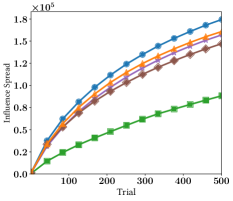
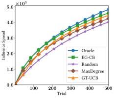
Baselines. We compare GT-UCB to several baselines. Random chooses a random influencer at each round. MaxDegree selects the node with the largest degree at each step $i$, where the degree does not include previously activated nodes. Finally, EG corresponds to the confidence-bound explore-exploit method with exponentiated gradient update from [24]; it is the state-of-the-art method for the OIMP problem (code provided by the authors). We use this last baseline on WC and TV weighted graphs and tune parameters in accordance to the results of their experiments: Maximum Likelihood Estimation is adopted for graph update and edge priors are set to Beta($1,20$). Note that EG learns parameters for the IC model, and hence is not applicable for LT. These baselines are compared to an Oracle that knows beforehand the diffusion model together with probabilities. At each round, it runs an influence maximization approximated algorithm – PMC for IC propagation, SSA for LT. Note that previously activated nodes are not counted when estimating the value of a node with PMC or SSA, thus, making Oracle an adaptive strategy.

All experiments are done by fixing the trial horizon $N=500$, a setting that is in line with many real-world marketing campaigns, which are fairly short and do not aim to reach the entire population.

(a) HepPh (WC – Impact of $K$)

(b) HepPh (WC – Influencer extraction)

(c) DBLP (WC – Impact of $K$)

(d) DBLP (WC – Influencer extraction)

Figure 4: Impact of $K$ and the influencer extraction criterion on influence spread.

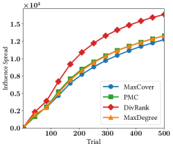
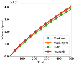
Choice of the influencers. We show in Fig. 4b and 4d the impact of the influencer extraction criterion on HepPh and DBLP under WC model. We can observe that the spread is only slightly affected by the extraction criterion: different datasets lead to different optimal criteria. On the HepPh network, DivRank clearly leads to larger influence spreads. On DBLP, however, the extraction method has little impact on resulting spreads. We emphasize that on some other graph and model combinations we observed that other extraction routines can perform better than DivRank. In summary, we note that GT-UCB performs consistently as long as the method leads to influencers that are well spread over the graph. In the following, for each graph, we used DivRank as the influencer extraction criterion in accordance with these observations.

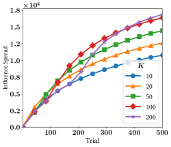
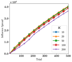
In Fig. 4a and 4c, we measure the impact of the number of influencers $K$ on the influence spread. We can observe that, on DBLP, a small number of influencers is sufficient to yield high-quality results. If too many influencers (relative to the budget) are selected (e.g. $K=200$), the initialization step required by GT-UCB is too long relative to the full budget, and hence GT-UCB does not reach its optimal spread – some influencers still have a large remaining potential at the end. On the other hand, a larger amount of influencers leads to greater influence spreads on HepPh: this network is relatively small ($34.5K$ nodes), and thus half of the nodes are already activated after $400$ trials. By having more influencers, we are able to access parts of the network that would not be accessible otherwise.

Figure 5: DBLP (WC) – Execution time.

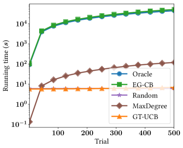
GT-UCB vs. baselines. We evaluate the execution time of the different algorithms in Fig. 5. As expected, GT-UCB largely outperforms EG (and Oracle). The two baselines require the execution of an approximated influence maximization algorithm at each round. In line with [2], we observed that SSA has prohibitive computational cost when incoming edge weights do not sum up to $1$, which is the case with both WC and TV. Thus, both Oracle and EG run PMC on all our experiments with IC propagation. GT-UCB is several orders of magnitude faster: it concentrates most of its running time on extracting influencers, while statistic updates and UCB computations are negligible.

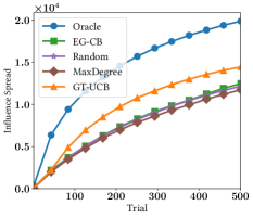
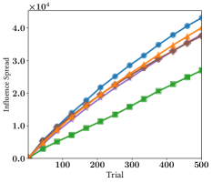
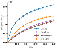
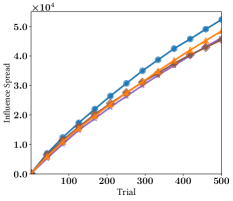
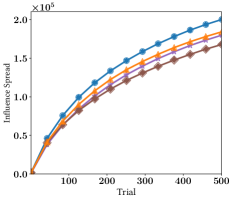
In Fig. 6, we show the growth of the spread for GT-UCB and baselines. For each experiment, GT-UCB uses $K=50$ if $L=1$ and $K=100$ if $L=10$. First, we can see that MaxDegree is a strong baseline in many cases, especially for WC and LT. GT-UCB results in good quality spreads across every combination of network and diffusion model. Interestingly, on the smaller graph HepPh, we observe an increase in the slope of spread after initialization, particularly visible at $t=50$ with WC and LT. This corresponds to the step when GT-UCB starts to select influencers maximizing $b_{k}(t)$ in the main loop. It shows that our strategy adapts well to the previous activations, and chooses good influencers at each iteration. Interestingly, Random performs surprisingly well in many cases, especially under TV weight assignment. However, when certain influencers are significantly better than others, it cannot adapt to select the best influencer unlike GT-UCB. EG performs well on HepPh, especially under TV weight assignment. However, it fails to provide competitive cumulative spreads on DBLP. We believe that EG tries to estimate too many parameters for a horizon $T=500$. After reaching this time step, less than $10\%$ of all nodes for WC, and $20\%$ for TV, are activated. This implies that we have hardly any information regarding the majority of edge probabilities, as most nodes are located in parts of the graph that have never been explored.

(a) HepPh (WC – $L=1$)

(b) DBLP (WC – $L=1$)

(c) DBLP (WC – $L=10$)

(d) HepPh (TV – $L=1$)

(e) DBLP (TV – $L=1$)

(f) DBLP (TV – $L=10$)

(g) HepPh (LT – $L=1$)

(h) DBLP (LT – $L=1$)

(i) DBLP (LT – $L=10$)

Figure 6: Growth of spreads against the number of rounds.

6.3 Experiments on Twitter

We continue the experimental section with an evaluation of GT-UCB on the Twitter data, introduced as a motivating example in Section 3. The interest of this experiment is to observe actual spreads, instead of simulated ones, over data that does not provide an explicit influence graph.

Figure 7: Twitter spread against rounds: (left) $L=1$ (right) $L=10$.

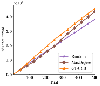
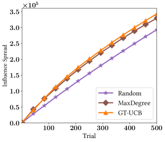
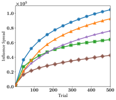
From the retweeting logs, for each active user $u$ – a user who posted more than $10$ tweets – we select users having retweeted at least one of $u$’s tweets. By doing so, we obtain the set of potentially influenceable users associated to active users. We then apply the greedy algorithm to select the users maximizing the corresponding set cover. These are the influencers of GT-UCB and Random. MaxDegree is given the entire reconstructed network (described in Table 1), that is, the network connecting active users to re-tweeters.

To test realistic spreads, at each step, once an influencer is selected by GT-UCB, a random cascade initiated by that influencer is chosen from the logs and we record its spread. This provides realistic, model-free spread samples to the compared algorithms. Since Twitter only contains successful activations (re-tweets) and not the failed ones, we could not test against EG, which needs both kinds of feedback.

In Fig. 7, we show the growth of the diffusion spread of GT-UCB against MaxDegree and Random. Again, GT-UCB uses $K=50$ if $L=1$ and $K=100$ if $L=10$. We can see that GT-UCB outperforms the baselines, especially when a single node is selected at each round. We can observe that MaxDegree performs surprisingly well in both experiments. We emphasize that it relies on the knowledge of the entire network reconstructed from retweeting logs, whereas GT-UCB is only given a set of (few) fixed influencers.

6.4 Influencer fatigue

We conclude the experimental section with a series of experiments on Twitter data and taking into account influencer fatigue.

In a similar way to Section 6.3, we compute the set of potentially influenceable users (the support) associated to all active users – the set of all users who retweeted at least one tweet from the active user. We then choose 20 influencers as follows: we take the 5 best influencers, that is, the 5 active users with the largest support; then, the 51st to 55th best influencers, then, the 501st to 505th best influencers, and finally the 5 worst influencers. By doing so, we obtain a set of 20 influencers with diverse profiles, roughly covering the possible influencing outcomes. Ideally, a good algorithm that takes into account influencer fatigue, would need to focus on the 5 best influencers at the beginning, but would need to move to other influencers when the initially optimal ones start to lose influence due to fatigue.

Figure 8: Fat-GT-UCB vs competitors on Twitter logs with (left) $\gamma_{1}$, (right) $\gamma_{2}$.

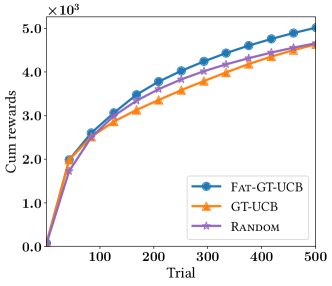
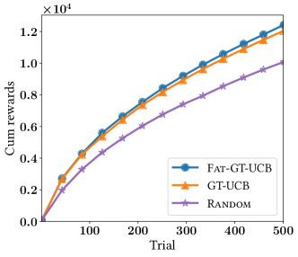
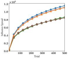
We compare Fat-GT-UCB to GT-UCB, which does not use the influence fatigue function, and to the Random baseline. As in Section 6.3, when an algorithm selects an influencer, we can choose a random spread from the logs (belonging to the selected influencer), and we can now simulate the fatigue by removing every user in the spread with probability $\gamma(n)$, where $n$ is the number of times the influencer has already been played.

We show the results of this comparison in Fig. 8. We tested with two different weariness functions, namely $\gamma_{1}(n)=1/n$ and $\gamma_{2}(n)=1/\sqrt{n}$. We can see that, in both scenarios, Fat-GT-UCB performs the best, showing that our UCB-like approach can effectively handle the notion of influencer fatigue in the OIMP problem. Unsurprisingly, GT-UCB performs better with weariness function $\gamma_{2}$ than is does with $\gamma_{1}$: the former has a lower diminishing impact and thus, the penalty of not incorporating fatigue is less problematic with $\gamma_{2}$.

7 Other related work

We have already discussed in Section 1 the main related studies in the area of influence maximization. For further details, we refer the interested reader to the recent survey in [2], which discusses the pros and cons of the best known techniques for influence maximization. In particular, the authors highlight that the Weighted Cascade (WC) instance of IC, where the weights associated to a node’s incoming edges must sum to one, leads to poor performance for otherwise rather fast IC algorithms. They conclude that PMC [31] is the state-of-the-art method to efficiently solve the IC optimization problem, while TIM+ [36] and IMM [35] – later improved by [30] with SSA – are the best current algorithms for WC and LT models.

Other methods have been devised to handle the prevalent uncertainty in diffusion media, e.g., when replacing edge probability scores with ranges thereof, by solving an influence maximization problem whose robust outcome should provide some effectiveness guarantees w.r.t. all possible instantiations of the uncertain model [20, 9].

Methods for influence maximization that take into account more detailed information, such as topical categories, have been considered in the literature [11, 3, 39]. Interestingly, [32] experimentally validates the intuition that different kinds of information spread differently in social networks, by relying on two complementary properties, namely stickiness and persistence. The former can be seen as a measure of how viral the piece of information is, passing from one individual to the next. The latter can be seen as an indicator of the extent to which repeated exposures to that piece of information impact its adoption, and it was shown to characterize complex contagions, of controversial information (e.g., from politics).

8 Conclusion

We propose in this paper a diffusion-independent approach for online and adaptive influencer marketing, whose role is to maximize the number of activated nodes in an arbitrary environment, under the OIMP framework. We focus on scenarios motivated by influencer marketing, in which campaigns consist of multiple consecutive trials conveying the same piece of information, requiring as only interfaces with the “real-world” the identification of potential seeds (the influencers) and the spread feedback (i.e., the set of activated nodes) at each trial. Our method’s online iterations are very fast, making it possible to scale to very large graphs, where other approaches become infeasible. The efficiency of GT-UCB comes from the fact that it only relies on an estimate of a single quantity for each influencer – its remaining potential. This novel approach is shown to be very competitive on influence maximization benchmark tasks and on influence spreads in Twitter. Finally, we extend our method to scenarios where, during a marketing campaign, the influencers may have a diminishing tendency to activate their user base.

Appendix A Useful Lemmas

Lemma 2 (Bennett’s inequality (Theorem 2.9 and 2.10 [5])).

Let $X_{1},\ldots,X_{n}$ be independent random variables with finite variance such that $X_{i}\leq b$ for some $b>0$ for all $i\leq n$. Let $S:=\sum_{i=1}^{n}\left(X_{i}-\mathbb{E}[X_{i}]\right)$ and $v:=\sum_{i=1}^{n}\mathbb{E}[X_{i}^{2}]$. Writing $\phi(u)=e^{u}-u-1$, then for all $t>0$,

$$\log\mathbb{E}\left[e^{tS}\right]\leq\frac{v}{b^{2}}\phi(bt)\leq\frac{vt^{2}}{2(1-bt/3)}.$$

This implies that, $\mathbb{P}\left(S>\sqrt{2v\log\nicefrac{{1}}{{\delta}}}+\frac{b}{3}\log\nicefrac{{1}}{{\delta}}\right)\leq\delta$.

Lemma 3 (Lemma 7 – [4]).

Let $n\geq 1$, $\lambda\geq 0$, $p\in[0,1]$ and $q=(1-p)^{n}$. Then,

$$qe^{\lambda p(1-q)}+(1-q)e^{-\lambda pq}\leq\exp(p\lambda^{2}/(4n))$$ (5)

$$qe^{\lambda p(q-1)}+(1-q)e^{\lambda pq}\leq\exp(p\lambda^{2}/(4n))$$ (6)

Appendix B Analysis of the Waiting Time of GT-UCB Algorithm

Lemma 4.

For any $s\geq 3$, $\mathbb{P}\left(\hat{R}_{s}\leq\hat{R}_{s-1}-\frac{\lambda}{e(s-2)}-\sqrt{\frac{2\lambda}{s-1}\log(1/\delta)}-\frac{1}{3(s-1)}\log(1/\delta)\right)\leq\delta.$

Proof.

Denote by $X_{s}(x):=\frac{U_{s-1}(x)}{s-1}-\frac{U_{s}(x)}{s}\leq\frac{1}{s-1}$. We can rewrite $\hat{R}_{s-1}-\hat{R}_{s}=\sum_{x\in A}X_{s}(x)$ and can easily verify that

$$v(x):=\mathbb{E}\left[X_{s}(x)^{2}\right]=p(x)(1-p(x))^{s-2}\left(\frac{1}{s-1}-\frac{1-p(x)}{s}\right)\leq\frac{p(x)}{s-1}.$$ (7)

Let $t>0$. By applying Lemma2, one obtains

$$\mathbb{P}\left(\hat{R}_{s-1}-\hat{R}_{s}\geq\mathbb{E}\left[\hat{R}_{s-1}-\hat{R}_{s}\right]+\sqrt{\frac{2\lambda}{s-1}\log(1/\delta)}+\frac{1}{3(s-1)}\log(1/\delta)\right)\leq\delta.$$

We conclude remarking that $\mathbb{E}[X_{s}(x)]=p(x)^{2}(1-p(x))^{s-2}\leq\frac{p(x)}{e(s-2)}$, that is, $\mathbb{E}[\hat{R}_{s-1}-\hat{R}_{s}]\leq\frac{\lambda}{e(s-2)}$. ∎

Theorem 3 (Waiting time).

Denote $\lambda^{\text{min}}:=\min_{k\in[K]}\lambda_{k}$ and $\lambda^{\text{max}}:=\max_{k\in[K]}\lambda_{k}$. Assume that $\lambda^{\text{min}}\geq 13$. Then, for any $\alpha\in\left[\frac{13}{\lambda\text{min}},1\right]$, if we define $\tau^{*}:=T^{*}\left(\alpha-\frac{13}{\lambda^{\text{min}}}\right)$, with probability at least $1-\frac{2K}{\lambda^{\text{max}}}$,

$$T_{\text{UCB}}(\alpha)\leq\tau^{*}+K\lambda^{\text{max}}\log(4\tau^{*}+11K\lambda^{\text{max}})+2K.$$

Proof.

Let us define the following confidence bounds:

$$b^{+}_{k,s}(t) :=(1+\sqrt{2})\sqrt{\frac{3\lambda_{k}\log(2t)}{s}}+\frac{\log(2t)}{s},$$

$$b^{-}_{k,s}(t) :=(1+\sqrt{2})\sqrt{\frac{3\lambda_{k}\log(2t)}{s}}+\frac{\log(2t)}{s}+\frac{\lambda_{k}}{s}\text{, and}$$

$$c^{-}_{k,t}(t) :=\frac{\lambda}{e(s-2)}+\sqrt{\frac{6\lambda_{k}\log(t)}{s-1}}+\frac{\log(t)}{s-1}.$$

Let $S>0$. Using these definitions, we introduce the following events:

$$\mathcal{F} :=\left\{\forall k\in[K],\forall t>S,\forall s\leq t,\hat{R}_{k,s}-b^{-}_{k,s}(t)\leq R_{k,s}\leq\hat{R}_{k,s}+b^{+}_{k,s}(t)\right\},$$

$$\mathcal{G} :=\left\{\forall k\in[K],\forall s\geq S,\hat{R}_{k,s}\geq\hat{R}_{k,s-1}-c^{-}_{k,s}(t)\right\},$$

$$\mathcal{E} :=\mathcal{F}\cap\mathcal{G}.$$

Using Theorem 1, Lemma 4 and a union bound, one obtains $\mathbb{P}(\mathcal{E})\geq 1-\frac{2K}{S}$ (by setting $\delta\equiv\frac{1}{t^{3}}$). Indeed,

$$\mathbb{P}\left(\bar{\mathcal{E}}\right)\leq\mathbb{P}(\bar{\mathcal{F}})+\mathbb{P}(\bar{\mathcal{G}})\leq 2\sum_{k=1}^{K}\sum_{t>S}\sum_{s\leq t}\frac{1}{t^{3}}=2K\sum_{t>S}\frac{1}{t^{2}}\leq\frac{2K}{S}.$$

In the following, we work on the event $\mathcal{E}$. Recall that we want to control $T_{UCB}(\alpha)$, the time at which every influencer attains a remaining potential smaller than $\alpha$ following GT-UCB strategy. We aim at comparing $T_{UCB}(\alpha)$ to $T^{*}(\alpha)$, the same quantity following the omniscient strategy. With that in mind, one can write:

$$T_{UCB}(\alpha)=\min\left\{t:\forall k\in[K],R_{k,N_{k}(t)}\leq\alpha\lambda_{k}\right\},$$

$$T^{*}(\alpha)=\sum_{k=1}^{K}T^{*}_{k}(\alpha)\text{, where }T^{*}_{k}(\alpha)=\min\left\{s:R_{k,s}\leq\alpha\lambda_{k}\right\}.$$

Following ideas from [8], we can control $T_{UCB}(\alpha)$ by comparing it to $U(\alpha)$ defined below, and which replaces the remaining potential by an upper bound on the estimator of the remaining potential (the Good-Turing estimator). Indeed, recall that we can control this on event $\mathcal{F}$.

$$U(\alpha)=\min\left\{t\geq 1:\forall k\in[K],\hat{R}_{k,N_{k}(t)}+b^{+}_{k,N_{k}(t)}(t)\leq\alpha\lambda_{k}\right\}.$$

Let $S^{\prime}\geq S$. On event $\mathcal{E}$, one has that $T_{UCB}(\alpha)\leq\max(S^{\prime},U(\alpha))$. If $U(\alpha)\geq S^{\prime}$, one has

$$R_{k,N_{k}(U(\alpha))} \geq\hat{R}_{k,N_{k}(U(\alpha))}-b^{-}_{k,N_{k}(U(\alpha))}(U(\alpha)) \mathcal{F} U(\alpha)>S^{\prime}\geq S$$ (we are on event and )

$$\geq\hat{R}_{k,N_{k}(U(\alpha))-1}-b^{-}_{k,N_{k}(U(\alpha))}(U(\alpha))-c^{-}_{k,N_{k}(U(\alpha))}(U(\alpha)) \mathcal{G}$$ (where are on event )

$$\geq\left(\alpha\lambda_{k}-b^{+}_{k,N_{k}(U(\alpha))-1}(U(\alpha))\right)-b^{-}_{k,N_{k}(U(\alpha))}(U(\alpha))-c^{-}_{k,N_{k}(U(\alpha))}(U(\alpha))$$

The third inequality’s justification is more evolved. Let $t$ be the time such that $N_{k}(t)=N_{k}(U(\alpha))-1$ and $N_{k}(t+1)=N_{k}(U(\alpha))$. This implies that $k$ is the chosen expert at time $t$, that is, the one maximizing the GT-UCB index. Moreover, since $t<U(\alpha)$, one knows that this index is greater than $\alpha\lambda_{k}$.

If $N_{k}(U(\alpha))\geq S^{\prime}+2$, some basic calculations lead to

$$R_{k,N_{k}(U(\alpha))}\geq\alpha\lambda_{k}-11\sqrt{\frac{\lambda_{k}\log(2U(\alpha))}{S^{\prime}}}-\frac{3\log(2U(\alpha))}{S^{\prime}}-\frac{3\lambda_{k}}{2S^{\prime}}$$

We denote by $\lambda^{max}:=\max_{k}\lambda_{k}$. If we take $S^{\prime}=\lambda^{max}\log(2U(\alpha))$, we can rewrite the previous inequality as

$$R_{k,N_{k}(U(\alpha))}\geq\alpha\lambda_{k}-11-\frac{3}{\lambda^{max}}-\frac{3}{2}$$

Thus, by definition of $T^{*}_{k}(\alpha)$, and if $\lambda^{max}>6$, one gets

$$N_{k,U(\alpha)}\leq T_{k}^{*}\left(\alpha-\frac{13}{\lambda_{k}}\right)+S^{\prime}+2.$$

Finally, if we denote by $\lambda^{min}=\min_{k}\lambda_{k}$, we obtain that

$$U(\alpha) \leq K(S^{\prime}+2)+T^{*}\left(\alpha-\frac{13}{\lambda^{min}}\right).$$

We now apply Lemma 5. We obtain that

$$U(\alpha)\leq 2K+\tau^{*}+K\lambda^{max}\log\left(8K+4\tau^{*}+10K\lambda^{max}\right)\leq\tau^{*}+K\lambda^{max}\log\left(4\tau^{*}+11K\lambda^{max}\right)+2K.$$

We conclude with $T_{UCB}(\alpha)\leq\max(S^{\prime},U(\alpha))$. ∎

Lemma 5 (Lemma 3 from [8]).

Let $a>0$, $b\geq 0.4$, and $x\geq e$, such that $x\leq a+b\log x$. Then one has

$$x\leq a+b\log(2a+4b\log(4b)).$$

Moreover, we add that if $b\geq 3$, then $x\leq a+b\log(2a+5b)$.

Appendix C Confidence intervals in the influencer fatigue setting

In this section, we consider a single influencer and omit its index $k$. We recall that we make the assumption that influencers have non-intersecting support. Thus, after selecting the influencer $n$ times, the remaining potential can be rewritten

$$R_{n}=\sum_{u\in A}\mathds{1}\{u\text{ never activated }\}p_{n+1}(u),$$

– $n+1$ because this is the remaining potential for the $n+1$th spread – and the corresponding Good-Turing estimator is

$$\hat{R}_{n}=\frac{1}{n}\sum_{u\in A}U^{\gamma}_{n}(u),$$

where $U^{\gamma}_{n}(u)=\sum_{i=1}^{n}\mathds{1}\{X_{1}=\ldots=X_{i-1}=X_{i+1}=\ldots=X_{n}=0,X_{i}=1\}\frac{\gamma(n+1)}{\gamma(i)}$.

Estimator bias.

Lemma 6 shows that the estimator of the remaining potential for the influencer fatigue setting is hardly biased.

Lemma 6.

Denoting $\lambda=\sum_{u\in A}p(u)$, the bias of the remaining potential estimator is

$$\mathbb{E}[R_{n}]-\mathbb{E}[\hat{R}_{n}]\in\left[-\gamma(n+1)\frac{\lambda}{n},0\right].$$

Proof.

We have that

$$\mathbb{E}[U^{\gamma}_{n}(u)]=\sum_{i=1}^{n}p_{i}(u)\prod_{j\neq i}(1-p_{j}(u))\frac{\gamma(n+1)}{\gamma(i)}=p_{n+1}(u)\sum_{i=1}^{n}\prod_{j\neq i}(1-p_{j}(u)).$$

We now can compute the bias of the estimator:

$$\mathbb{E}[R_{n}]-\mathbb{E}[\hat{R}_{n}] =\frac{1}{n}\sum_{u\in A}p_{n+1}(u)\left[\sum_{i=1}^{n}\prod_{j=1}^{n}(1-p_{j}(u))-\sum_{i=1}^{n}\prod_{j\neq i}(1-p_{j}(u))\right]$$

$$=\frac{1}{n}\sum_{u\in A}p_{n+1}(u)\sum_{i=1}^{n}\prod_{j\neq i}(1-p_{j}(u))[1-p_{i}(u)-1]$$

$$=-\frac{1}{n}\sum_{u\in A}p_{n+1}(u)\sum_{i=1}^{n}p_{i}(u)\prod_{j\neq i}(1-p_{j}(u))$$

$$=-\frac{1}{n}\mathbb{E}\left[\sum_{u\in A}p_{n+1}(u)U_{n}(u)\right]\in\left[-\frac{\sum_{u\in A}p_{n+1}(u)}{n},0\right]$$

Note that the random variable $U_{n}(u)$ correspond to the hapax definition given in the original OIMP problem, that is, $U_{n}(u)=\mathds{1}\{u\text{ activated exactly once}\}$. ∎

Unsurprisingly, we obtain the same bias for the case where $\gamma$ is constant equal to 1 (no fatigue).

Confidence Intervals.

To derive an optimistic algorithm, we need confidence intervals on the remaining potential. We operate in three steps:

1. Good-Turing deviations: Remember that $\hat{R}_{n}=\sum_{u\in A}\frac{U_{n}^{\gamma}(u)}{n}$. We have next that

   $$\mathbb{E}[U_{n}^{\gamma}(u)^{2}] =\sum_{i=1}^{n}p_{i}(u)\prod_{j\neq i}(1-p_{j}(u))\frac{\gamma(n+1)^{2}}{\gamma(i)^{2}}$$

   $$=\sum_{i=1}^{n}p_{n+1}(u)\prod_{j\neq i}(1-p_{j}(u))\frac{\gamma(n+1)}{\gamma(i)}$$

   $$\leq np(u)\gamma(n+1).$$

   Thus, we have that $v:=\sum_{u\in A}\mathbb{E}\left[\frac{U^{\gamma}_{n}(u)^{2}}{n^{2}}\right]\leq\frac{\sum_{u\in A}p_{n+1}(u)}{n}$.

   Applying Bennett’s inequality to the independent random variables $\{X^{\gamma}_{n}(u)\}_{u\in A}$ yields

   $$\mathbb{P}\left(\hat{R}_{n}-\mathbb{E}\left[\hat{R}_{n}\right]\geq\sqrt{\frac{2\lambda_{n+1}\log(1/\delta)}{n}}+\frac{1}{3n}\log(1/\delta)\right)\leq\delta,$$ (8)

   where $\lambda_{n}:=\gamma(n)\sum_{u\in A}p(u)$.

   The same inequality can be derived for left deviations.

2. Remaining potential deviations: Remember that $R_{n}=\sum_{u\in A}Z_{n}(u)p_{n+1}(u)$ where $Z_{n}(u)=\mathds{1}\{u\text{ never activated}\}=\mathds{1}\{X_{1}(u)=\cdots=X_{n}(u)=0\}$. We denote $Y_{n}(u)=p_{n+1}(u)(Z_{n}(u)-\mathbb{E}[Z_{n}(u)])$ and $q_{n}(u)=\mathbb{P}(Z_{n}(u)=1)=\prod_{i=1}^{n}(1-p_{s}(u))$. We have that

   $$\mathbb{P}\left(R_{n}-\mathbb{E}[R_{n}]\geq\epsilon\right) \leq e^{-t\epsilon}\prod_{u\in A}\mathbb{E}\left[e^{tY_{n}(u)}\right]$$

   $$=e^{-t\epsilon}\prod_{u\in A}\left(\mathbb{P}(Z_{n}(u)=1)e^{tp_{n+1}(u)(1-q_{n}(u))}+\mathbb{P}(Z_{n}(u)=0)e^{-tp_{n+1}(u)q_{n}(u)}\right)$$

   $$=e^{-t\epsilon}\prod_{u\in A}\left(q_{n}(u)e^{tp_{n+1}(u)(1-q_{n}(u))}+(1-q_{n}(u))e^{-tp_{n+1}(u)q_{n}(u)}\right)$$

   $$\leq e^{-t\epsilon}\prod_{u\in A}\exp\left(\frac{p_{n+1}(u)t^{2}}{4n}\right)$$ (by Eq. 9 in Lemma 7)

   Minimizing on $t$, we obtain (for $t=\frac{2\epsilon n}{\sum_{u\in A}p_{n+1}(u)})$,

   $$\mathbb{P}\left(R_{n}-\mathbb{E}[R_{n}]\geq\epsilon\right)\leq\exp\left(\frac{-\epsilon^{2}n}{\sum_{u\in A}p_{n+1}(u)}\right).$$

   We can proceed similarly to obtain the left deviation.

Putting it all together, we obtain the following confidence intervals in Theorem 4, which can be used in the design of the optimistic algorithm Fat-GT-UCB.

Theorem 4.

With probability at least $1-\delta$, for $\lambda_{n}=\gamma(n)\sum_{u\in A}p(u)$ and $\beta_{n}:=\left(1+\sqrt{2}\right)\times\sqrt{\frac{\lambda_{n+1}\log(4/\delta)}{n}}+\frac{1}{3n}\log\frac{4}{\delta}$, the following holds:

$$-\beta_{n}-\frac{\lambda}{n}\leq R_{n}-\hat{R}_{n}\leq\beta_{n}.$$

Lemma 7 (Adaptation of Lemma 3.5 in [4]).

Let $n\geq 1$, $p\in[0,1]$, $\gamma:\mathbb{N}\to[0,1]$ a non-increasing function and $t\geq 0$. We denote $p_{n}=\gamma(n)p$ and $q_{n}=\prod_{i\leq t}(1-p_{i})$.

$$(a)~{}~{}q_{n}e^{tp_{n}(1-q_{n})}+(1-q_{n})e^{-tp_{n}q_{n}}\leq\exp\left(\frac{p_{n}t^{2}}{4n}\right)$$ (9)

$$(b)~{}~{}q_{n}e^{tp_{n}(q_{n}-1)}+(1-q_{n})e^{tp_{n}q_{n}}\leq\exp\left(\frac{p_{n}t^{2}}{4n}\right)$$ (10)

Proof.

Let $q_{n}^{\prime}=(1-p_{n})^{n}$. Clearly, $q_{n}\leq q_{n}^{\prime}$.

(a) Using Theorem 3.2 in [4] with $p\equiv q_{n}$ and $t\equiv tp_{n}$, we have that,

$$q_{n}e^{tp_{n}(1-q_{n})}+(1-q_{n})e^{-tp_{n}q_{n}}\leq\exp\left(\frac{1-2q_{n}}{4\log((1-q_{n})/q_{n})}t^{2}p_{n}^{2}\right).$$

So it suffices to show that

$$(1-2q_{n})t^{2}p_{n}^{2}/4\log((1-q_{n})/q_{n})\leq p_{n}t^{2}/4n,$$

or equivalently,

$$(1-2q_{n})p_{n}\log((1-q_{n})/q_{n})\leq\log(1-p_{n})/\log(q_{n}^{\prime}).$$

Rearranging, we obtain,

$$L(q_{n},q_{n}^{\prime}):=\frac{(1-2q_{n})\log(1/q_{n}^{\prime})}{\log((1-q_{n})/q_{n})}\leq\frac{1/\log(1-p_{n})}{p_{n}}:=R(p_{n}).$$

As is [4], we show that $L\leq 1\leq R$. The second inequality is true (see [4]).

The left-hand side can be written $L(q_{n},q_{n}^{\prime})=L_{1}(q_{n})L_{2}(q_{n}^{\prime})$. Clearly, $L_{2}(q_{n}^{\prime})\geq 0$. If $L_{1}(q_{n})\leq 0$, the left-hand side is negative and thus, $L(q_{n},q_{n}^{\prime})\leq 1$. Else, $L_{1}(q_{n})\geq 0$, we can upper bound the right-hand side as $L(q_{n},q_{n}^{\prime})\leq\frac{(1-2q_{n})\log(1/q_{n})}{\log((1-q_{n})/q_{n})}$ (because $q_{n}\leq q_{n}^{\prime}$), which is proven to be less than $1$ in [4]. This concludes the proof.

(b) It is shown in the proof Lemma 3.5 (b) in [4] that

$$L(t):=\frac{1}{t^{2}p_{n}^{2}}\log\left[q_{n}e^{-tp_{n}(1-q_{n})}+(1-q_{n})e^{tp_{n}q_{n}}\right]\leq\frac{1}{t^{2}p_{n}^{2}}\frac{t^{2}p_{n}}{4\log q_{n}/\log(1-p_{n})}=:R(q_{n}).$$

It suffices to show that $R(q_{n})\leq R(q_{n}^{\prime})$ to obtain the desired inequality. This is true because

$$0\leq\frac{\log(1-p_{n})}{\log q_{n}}\leq\frac{\log(1-p_{n})}{\log q_{n}^{\prime}}.$$

∎

References

- [1] In Duncan Brown and Nick Hayes, editors, Influencer Marketing. Butterworth-Heinemann, Oxford, 2008.
- [2] A. Arora, S. Galhotra, and S. Ranu. Debunking the myths of influence maximization: An in-depth benchmarking study. In SIGMOD. ACM, 2017.
- [3] N. Barbieri, F. Bonchi, and G. Manco. Topic-aware social influence propagation models. Knowl. Inf. Syst., 37(3):555–584, 2013.
- [4] D. Berend and A. Kontorovich. On the concentration of the missing mass. In Electronic Communications in Probability, pages 1–7, 2013.
- [5] S. Boucheron, G. Lugosi, P. Massart, and M. Ledoux. Concentration inequalities : a nonasymptotic theory of independence. Oxford university press, 2013.
- [6] D. Brown and S. Fiorella. Influence Marketing: How to Create, Manage, and Measure Brand Influencers in Social Media Marketing. Always learning. Que, 2013.
- [7] S. Bubeck and N. Cesa-Bianchi. Regret analysis of stochastic and nonstochastic multi-armed bandit problems. Foundations & Trends in ML, 2012.
- [8] S. Bubeck, D. Ernst, and A. Garivier. Optimal discovery with probabilistic expert advice: finite time analysis and macroscopic optimality. Journal of Machine Learning Research, 14(1):601–623, 2013.
- [9] W. Chen, T. Lin, Z. Tan, M. Zhao, and X. Zhou. Robust influence maximization. In SIGKDD, pages 795–804, 2016.
- [10] W. Chen, Y. Wang, Y. Yuan, and Q. Wang. Combinatorial multi-armed bandit and its extension to probabilistically triggered arms. JMLR, 17(1), 2016.
- [11] N. Du, L. Song, H. Woo, and H. Zha. Uncover topic-sensitive information diffusion networks. In AISTATS, pages 229–237, 2013.
- [12] D. Easley and J. Kleinberg. Networks, Crowds, and Markets - Reasoning About a Highly Connected World. Cambridge University Press, 2010.
- [13] Paul Gillin. The New Influencers: A Marketer’s Guide to the New Social Media. Quill Driver Books, Sanger, CA, 2007.
- [14] M. Gomez-Rodriguez, D. Balduzzi, and B. Schölkopf. Uncovering the temporal dynamics of diffusion networks. In ICML, pages 561–568, 2011.
- [15] M. Gomez-Rodriguez, J. Leskovec, and A. Krause. Inferring networks of diffusion and influence. ACM Trans. Knowl. Discov. Data, 5(4), February 2012.
- [16] M. Gomez-Rodriguez, J. Leskovec, and B. Schölkopf. Structure and dynamics of information pathways in online media. In WSDM, pages 23–32, 2013.
- [17] I. J. Good. The population frequencies of species and the estimation of population parameters. Biometrika, 40(3-4):237, 1953.
- [18] A. Goyal, F. Bonchi, and L. Lakshmanan. Learning influence probabilities in social networks. In WSDM, pages 241–250, 2010.
- [19] P. Grabowicz, N. Ganguly, and K. Gummadi. Distinguishing between topical and non-topical information diffusion mechanisms in social media. In ICWSM, pages 151–160, 2016.
- [20] X. He and D. Kempe. Robust influence maximization. In SIGKDD, pages 885–894, 2016.
- [21] D. Kempe, J. Kleinberg, and É. Tardos. Maximizing the spread of influence through a social network. In SIGKDD, pages 137–146. ACM, 2003.
- [22] Paul Lagrée, Olivier Cappé, Bogdan Cautis, and Silviu Maniu. Effective large-scale online influence maximization. In ICDM, 2017.
- [23] Kamiu Lee. Influencer marketing 2.0: Key trends in 2017. https://influence.bloglovin.com/influencer-marketing-2-0-key-trends-in-2017-a5fb97424cd, 2017.
- [24] S. Lei, S. Maniu, L. Mo, R. Cheng, and P. Senellart. Online influence maximization. In SIGKDD, 2015.
- [25] Nir Levine, Koby Crammer, and Shie Mannor. Rotting bandits. In Advances in Neural Information Processing Systems 30 (NIPS), 2017.
- [26] Jonathan Louëdec, Laurent Rossi, Max Chevalier, Aurélien Garivier, and Josiane Mothe. Algorithme de bandit et obsolescence : un modèle pour la recommandation. 2016.
- [27] D. McAllester and L. Ortiz. Concentration inequalities for the missing mass and for histogram rule error. JMLR, 4:895–911, 2003.
- [28] D. McAllester and R. Schapire. On the convergence rate of good-turing estimators. In COLT, pages 1–6, 2000.
- [29] Q. Mei, J. Guo, and D. Radev. Divrank: The interplay of prestige and diversity in information networks. In SIGKDD, 2010.
- [30] H. T. Nguyen, M. T. Thai, and T. N. Dinh. Stop-and-stare: Optimal sampling algorithms for viral marketing in billion-scale networks. In SIGMOD, 2016.
- [31] N. Ohsaka, T. Akiba, Y. Yoshida, and K. Kawarabayashi. Fast and accurate influence maximization on large networks with pruned monte-carlo simulations. In AAAI, 2014.
- [32] D. Romero, B. Meeder, and J. Kleinberg. Differences in the mechanics of information diffusion across topics: Idioms, political hashtags, and complex contagion on twitter. In WWW, pages 695–704, 2011.
- [33] K. Saito, R. Nakano, and M. Kimura. Prediction of information diffusion probabilities for independent cascade model. In KES, pages 67–75, 2008.
- [34] Cole Sletten. How to prepare brands for influencer fatigue. https://www.forbes.com/sites/onmarketing/2017/01/24/how-to-prepare-brands-for-influencer-fatigue, 2017.
- [35] Y. Tang, Y. Shi, and X. Xiao. Influence maximization in near-linear time: A martingale approach. In SIGMOD, pages 1539–1554, 2015.
- [36] Y. Tang, X. Xiao, and Y. Shi. Influence maximization: Near-optimal time complexity meets practical efficiency. In SIGMOD, pages 75–86, 2014.
- [37] S. Vaswani, B. Kveton, Z. Wen, M. Ghavamzadeh, L. Lakshmanan, and M. Schmidt. Diffusion independent semi-bandit influence maximization. In ICML, 2017.
- [38] S. Vaswani, V.S. Lakshmanan, and M. Schmidt. Influence maximization with bandits. In Workshop NIPS, NIPS ’15, 2015.
- [39] S. Wang, X. Hu, P. Yu, and Z. Li. Mmrate: inferring multi-aspect diffusion networks with multi-pattern cascades. In SIGKDD, pages 1246–1255, 2014.
- [40] D. Watts. Six Degrees: The Science of a Connected Age. W. W. Norton, NY, 2003.
- [41] D. Watts and P. Dodds. Influentials, networks, and public opinion formation. Journal of Consumer Research, 34(4):441–458, 2007.
- [42] Z. Wen, B. Kveton, and M. Valko. Influence maximization with semi-bandit feedback. Technical report, 2016.