Periodic orbits in nonlinear wave equations on networks

Abstract

We consider a cubic nonlinear wave equation on a network and show that inspecting the normal modes of the graph, we can immediately identify which ones extend into nonlinear periodic orbits. Two main classes of nonlinear periodic orbits exist: modes without soft nodes and others. For the former which are the Goldstone and the bivalent modes, the linearized equations decouple. A Floquet analysis was conducted systematically for chains; it indicates that the Goldstone mode is usually stable and the bivalent mode is always unstable. The linearized equations for the second type of modes are coupled, they indicate which modes will be excited when the orbit destabilizes. Numerical results for the second class show that modes with a single eigenvalue are unstable below a treshold amplitude. Conversely, modes with multiple eigenvalues seem always unstable. This study could be applied to coupled mechanical systems.

I Introduction

Linearly coupled mechanical systems are well understood in terms of normal modes, see landau . These are bound states of the Hamiltonian which is a quadratic, symmetric function of positions and velocities. The bound states are orthogonal and correspond to real frequencies. Because of the orthogonality, normal modes do not couple and the system can be described solely in terms of the amplitude of each mode and its time derivative. When non linearity is present in the equations of motion, normal modes will couple. Natural questions are : how do they couple ? Is there any trace of them in the nonlinear regime? An important realisation is that some systems exhibit nonlinear periodic solutions. The situation differs whether the degrees of freedom are nonlinear and coupled linearly or whether they are linear oscillators coupled nonlinearly as in the celebrated Fermi-Pasta-Ulam model fpu .

Nonlinear oscillators coupled linearly can give rise to periodic solution labeled "intrinsic localized modes", see the reviews flach98 ; flach08 . These are nonlinear periodic orbits that are exponentially localized in a region of the lattice. For large amplitudes, these solutions are in general different from the linear normal modes. Another type of nonlinear periodic orbit can exist, which is a continuation of the linear normal modes panos . For the Fermi-Pasta-Ulam system, this type of nonlinear periodic orbit has been found using group theoretical methods and Hamiltonian perturbation methods cr12 ; crz05 ; bcs11 . Also, in the theoretical mechanics community, such linear-nonlinear periodic orbits have been studied for some time, see the extensive review by am13 .

In a pioneering work, for one dimensional lattices with linear coupling and onsite nonlinearity, i.e. nonlinear oscillators coupled linearly, Aoki aoki recently found families of nonlinear periodic orbits stemming from the linear normal modes. He studied one dimensional lattices with periodic, fixed or free boundary conditions. His main findings are that normal modes with coordinates containing $\pm 1$ and $0$ give rise to nonlinear periodic orbits. Analysis of their dynamical stability revealed that the modes containing only $\pm 1$ lead to decoupled variational equations, one for each normal mode.

In this article, we extend Aoki’s approach to general networks with linear couplings and onsite nonlinearity. The underlying linear model is the graph wave equation cks13 where the Laplacian is the graph Laplacian Cvetkovic1 . It is a natural description of miscible flows on a network since it arises from conservation laws. It also models the density when one considers a probabilistic motion on a graph. In a recent work cks13 , we studied this model and showed the importance of the normal modes, i.e. the eigenvectors of the Laplacian matrix and their associated real eigenvalues. We choose a cubic nonlinearity because the solution exists for all times, the evolution problem is well-posed. We extend the criterion of Aoki to any network; by inspecting the normal modes of a network we can immediately identify nonlinear periodic orbits. We give all such nonlinear periodic orbits for cycles and chains, these are the well-known Goldstone mode and what we call bivalent and trivalent modes. We also show examples in networks that are neither chains or cycles. Two main classes of modes exist, the ones with no zero nodes (the Goldstone and bivalent modes) and the others (trivalent modes). For the first class, the variational equations decouple completely into $N$ Hill-like resonance equations. For the second class, we give explicitely their form, enabling prediction of the couplings. It is surprising that the dynamics of periodic orbits is different when soft nodes are present. The special role of these soft nodes in the dynamics had been analyzed in cks13 . For the first class we calculate the stability diagram of the nonlinear periodic orbits systematically for chains. The Goldstone mode is usually stable for large enough amplitude. On the contrary the bivalent modes are always unstable. The second class is more difficult to study; it’s stability is governed by a system of coupled resonance equations. These reveal which new modes will be excited when there is instability. Numerical calculations illustrate these different situations. The fact that the nonlinear periodic orbits have an explicit solution, and the form of the linearization around some of these solutions are quite unique features of the model. We believe these results will be useful to the lattice community but also more generally to the theoretical mechanics community where these systems occur.
The article is organized as follows: We introduce the model in section 2. In section 3, we generalize the criterion of Aoki that shows which linear normal modes extend to nonlinear periodic orbits. Section 4 classifies these nonlinear normal modes for chains and cycles and gives other examples. Section 5 presents the variational equations obtained by perturbing the nonlinear normal modes. These are solved numerically for chains in section 6 for the Goldstone and the bivalent modes. Full numerical results are presented in section 7 for trivalent modes. Conclusions are presented in section 8.

II Amplitude equations

We consider the following nonlinear wave equation on a connected graph with $N$ nodes

$$\ddot{\mathbf{u}}=\mathbf{\Delta}\mathbf{u}-\mathbf{u}^{3},$$ (1)

where $\mathbf{u}=(u_{1}(t),\dots,u_{N}(t))^{T}$ is the field amplitude, $\mathbf{\Delta}$ is the graph Laplacian Cvetkovic1 with components $\Delta_{ij},~{}~{}1\leq i,j\leq N$, $\mathbf{u}^{3}=(u_{1}^{3},u_{2}^{3},\dots,u_{N}^{3})^{T}$ and where $\ddot{\mathbf{u}}\equiv{\mathrm{d}^{2}{\mathbf{u}}\over\mathrm{d}t^{2}}$. Notice that we use bold-face capitals for matrices and bold-face lower-case letters for vectors. This model is an extension to a graph of the simplified $\phi^{4}$ well-known model in condensed matter physics lattices Scott1 . This equation is the discrete analogous of the continuum model, see Strauss for a review of the well-posedness of the continuum model. Equation (1) can be seen as a discretisation of such a continuum model; it is therefore well-posed. The power of the nonlinearity is important to get a well-posed problem. This can be seen by omitting the Laplacian and looking at the differential equation $\ddot{\mathbf{u}}=-\mathbf{u}^{\alpha}$ whose solutions are bounded for $\alpha$ odd.

Since the graph Laplacian $\mathbf{\Delta}$ is a real symmetric negative-semi definite matrix, it is natural, following cks13 , to expand $\mathbf{u}$ using a basis of the eigenvectors $\mathbf{v}^{j}$ of $\mathbf{\Delta}$, such that

$$\mathbf{\Delta}\mathbf{v}^{j}=-\omega_{j}^{2}\mathbf{v}^{j}.$$ (2)

The vectors $\mathbf{v}^{j}$ can be chosen to be orthonormal with respect to the scalar product in $\mathbb{R}^{N}$, i.e. $\left\langle\mathbf{v}^{i},\mathbf{v}^{j}\right\rangle=\delta_{i,j}$ where $\delta_{i,j}$ is the Kronecker symbol, so the matrix $\mathbf{P}$ formed by the columns $\mathbf{v}^{j}$ is orthogonal. The relation (2) can then be written

$$\mathbf{\Delta}\mathbf{P}=\mathbf{P}\mathbf{D},$$

where $\mathbf{D}$ is the diagonal matrix of diagonal $-\omega_{1}^{2}=0>-\omega_{2}^{2}\geq\cdots\geq-\omega_{N}^{2}$. The first eigenfrequency $\omega_{1}=0$ (the graph is connected) corresponds to the Goldstone mode Scott2 whose components are equal on a network $\mathbf{v}^{1}={1\over\sqrt{N}}(1,1,\dots,1)^{T}$. We introduce the vector $\mathbf{a}=(a_{1},a_{2},..,a_{N})^{T}$ such that

$$\mathbf{u}=\mathbf{P}\mathbf{a}=\sum_{k=1}^{N}a_{k}\mathbf{v}^{k}.$$ (3)

In terms of the coordinates $a_{j}$, substituting (3) into (1) and projecting on each mode $\mathbf{v}^{j}$, we get the system of $N$-coupled ordinary differential equations

$$\ddot{a}_{j}=-\omega_{j}^{2}a_{j}-\sum_{m=1}^{N}u_{m}^{3}v_{m}^{j},~{}~{}j\in\{1,...,N\},$$

where we have used the orthogonality of the eigenvectors of $\mathbf{\Delta}$, $\mathbf{P}^{-1}=\mathbf{P}^{T}$. The term $u_{m}^{3}$ can be written as $u_{m}^{3}=\sum_{k,l,p=1}^{N}a_{k}a_{l}a_{p}v_{m}^{k}v_{m}^{l}v_{m}^{p}$. We get then a set of $n$ second order inhomogeneous coupled differential equations:

$$\ddot{a}_{j}+\omega_{j}^{2}a_{j}=-\sum_{k,l,p=1}^{N}\Gamma_{jklp}a_{k}a_{l}a_{p},$$ (4)

where

$$\Gamma_{jklp}=\sum_{m=1}^{N}{v}^{j}_{m}~{}{v}^{k}_{m}~{}{v}^{l}_{m}~{}{v}^{p}_{m}.$$ (5)

Notice that the graph geometry comes through the coefficients $\Gamma_{jklp}$. For a general graph, the spectrum needs to be computed numerically and these coefficients as well. For cycles and chains however, the eigenvalues and the eigenvectors of the Laplacian have an explicit formula (see Appendix A) so that $\Gamma_{jklp}$ can be computed explicitely. Then, we obtain the amplitude equations coupling the normal modes.

In our previous study cks13 , we noted the importance of nodes for which the component of the eigenvector is zero. We introduced "a soft node" as : a node $s$ of a graph is a soft node for an eigenvalue $-\omega_{j}^{2}$ of the graph Laplacian if there exists an eigenvector $\mathbf{v}^{j}$ for this eigenvalue such that ${v}^{j}_{s}=0$. On such soft nodes, any forcing or damping of the system is null for the corresponding normal mode cks13 .

III Existence of periodic orbits

In aoki , Aoki studied nonlinear periodic orbits for chain or cycle graphs, i.e. one dimensional lattices with free or periodic boundary conditions. He identified a criterion allowing to extend some linear normal modes into nonlinear periodic orbits for the $\phi^{4}$ model (cubic nonlinearity). In this section, we generalize Aoki’s criterion to any graph.

Let us find the conditions for the existence of a nonlinear periodic solution of (1) of the form

$$\mathbf{u}(t)=a_{j}(t)\mathbf{v}^{j},$$ (6)

the equations of motion (1) reduce to

$$\ddot{a}_{j}v_{m}^{j}=-\omega_{j}^{2}a_{j}v_{m}^{j}-a_{j}^{3}(v_{m}^{j})^{3}.$$ (7)

These equations are satisfied for the nodes $m$ such that $v_{m}^{j}=0$ (the soft nodes).
For $v_{m}^{j}\neq 0$, we can simplify (7) by $v_{m}^{j}$ and obtain

$$\ddot{a}_{j}=-\omega_{j}^{2}a_{j}-a_{j}^{3}(v_{m}^{j})^{2}.$$

These equations should be independant of $m$ and this imposes

$$(v_{m}^{j})^{2}=C,$$ (8)

where $C$ is a constant. Remembering that $\left\lVert\mathbf{v}^{j}\right\rVert=1$ we get

$$C={1\over N-S},$$

where $S$ is the number of soft nodes.

To summarize, for a general network, we identified nonlinear periodic orbits $\mathbf{u}^{j}(t)$ associated to a linear eigenvector $\mathbf{v}^{j}$ of the Laplacian; they are

$$\left\{\begin{array}[]{l c r}\mathbf{u}^{j}(t)=a_{j}(t)\mathbf{v}^{j},\\ \\ {1\over\sqrt{C}}v_{m}^{j}\in\{0,1,-1\},~{}~{}~{}\forall m\in\left\{1,\dots,N\right\},~{}~{}C={1\over N-S},\\ \\ \ddot{a}_{j}=-\omega_{j}^{2}a_{j}-Ca_{j}^{3}.\end{array}\right.$$ (9)

There are three kinds of nonlinear periodic orbits monovalent, bivalent and trivalent depending whether they contain one, two or three different values. The only monovalent orbit is the Goldstone mode. The bivalent orbits contain $+1,-1$ up to a normalization constant. Finally, the trivalent orbits are composed of $0,+1,-1$; they posess soft nodes.

Several remarks can be made. The first one is that the criterion can be generalized to any odd power of the nonlinearity. We can use the condition (8) to systematically find periodic orbits for a general nonlinear wave equation with a polynomial nonlinearity with odd powers $\mathcal{N}(\mathbf{u})=-\mathbf{u}^{3}-\mathbf{u}^{5}\dots$.
We have tried to obtain nonlinear quasi-periodic orbits of the form

$$\mathbf{u}(t)=a_{j}(t)\mathbf{v}^{j}+a_{k}(t)\mathbf{v}^{k}.$$

Preliminary results are shown in the Appendix B.

IV Examples of nonlinear periodic orbits

There are a number of examples which can be easily identified. First, consider the modes without soft nodes.

• The monovalent mode, also named zero linear frequency mode or Goldstone mode

  $$v_{m}^{1}={1\over\sqrt{N}},~{}~{}~{}\forall m\in\left\{1,\dots,N\right\},$$

  exists for any graph.

• The bivalent mode

  $$v_{m}^{j}=\pm{1\over\sqrt{N}},~{}~{}~{}\forall m\in\left\{1,\dots,N\right\},$$

  exists for chains with $N$ even and for $j={N\over 2}+1$,

  $$v_{m}^{{N\over 2}+1}={1\over\sqrt{N}}\left\{\begin{array}[]{l c r}(-1)^{m\over 2},\quad\text{if }m\text{ even},\\ \\ (-1)^{m-1\over 2},\quad\text{if }m\text{ odd},\\ \end{array}\right.$$

  corresponds to the frequency $\omega_{{N\over 2}+1}=\sqrt{2}$. For example, for a chain of $N=4$ nodes, we have the following bivalent mode

  

• For cycles with $N$ even, the bivalent mode $\mathbf{v}^{N}$ alternates, it is such that $v_{m}^{N}=-v_{m+1}^{N}$. It corresponds to the frequency $\omega_{N}=2$

  $$v_{m}^{N}={1\over\sqrt{N}}(-1)^{m-1},~{}~{}~{}\forall m\in\left\{1,\dots,N\right\}.$$

  For a cycle of $N=4$ nodes, we have the following bivalent mode

  

Other graphs that are neither a chain or a cycle can exhibit bivalent nonlinear modes. These are for example, using the classification of Cvetkovic1

• The Network 110 labeled as

  

  The nonlinear periodic orbit originates from the linear mode,

  $$\omega_{4}^{2}=2,~{}\mathbf{v}^{4}={1\over\sqrt{6}}(1,-1,-1,-1,1,1)^{T}.$$

• The network 105

  

  The nonlinear periodic orbit originates from the linear mode,

  $$\omega_{4}^{2}=2,~{}\mathbf{v}^{4}={1\over\sqrt{6}}(-1,-1,1,1,1,-1)^{T}.$$

Nonlinear modes containing soft nodes, or trivalent modes can be found in the following graphs:

• For chains with $N$ multiple of $3$, the mode $\mathbf{v}^{{N\over 3}+1}$ corresponds to the frequency $\omega_{N}=1$

  $$\sqrt{{2N\over 3}}v_{m}^{{N\over 3}+1}\in\{0,1,-1\},~{}~{}~{}\forall m\in\left\{1,\dots,N\right\}.$$

  Notice that $v_{m}^{{N\over 3}+1}=0$ for $m=3k+2$ and $k\in\{0,\dots,{N\over 3}-1\}$.

• For cycles where $N$ is multiple of $4$, we have a double frequency $\omega_{N\over 2}=\omega_{{N\over 2}+1}=\sqrt{2}$ and two eigenvectors

  $$v_{m}^{{N\over 2}}=\sqrt{2\over N}\left\{\begin{array}[]{l c r}0,\quad\text{if }m\text{ even},\\ \\ (-1)^{m-1\over 2},\quad\text{if }m\text{ odd}.\\ \end{array}\right.$$

  $$v_{m}^{{N\over 2}+1}=\sqrt{2\over N}\left\{\begin{array}[]{l c r}(-1)^{{m\over 2}+1},\quad\text{if }m\text{ even},\\ \\ 0,\quad\text{if }m\text{ odd}.\\ \end{array}\right.$$

• For cycles with $N$ multiple of $3$, the mode $\mathbf{v}^{{2N\over 3}+1}$ corresponds to the double frequency $\omega_{{2N\over 3}}=\omega_{{2N\over 3}+1}=\sqrt{3}$

  $$\sqrt{{2N\over 3}}v_{m}^{{2N\over 3}+1}\in\{0,1,-1\},~{}~{}~{}\forall m\in\left\{1,\dots,N\right\}.$$

  Notice that $v_{m}^{{2N\over 3}+1}=0$ for $m=3k+1$ and $k\in\{0,\dots,{N\over 3}-1\}$.

• For cycles with $N$ multiple of $6$, the mode $\mathbf{v}^{{N\over 3}+1}$ corresponds to the double frequency $\omega_{{N\over 3}}=\omega_{{N\over 3}+1}=1$

  $$\sqrt{{2N\over 3}}v_{m}^{{N\over 3}+1}\in\{0,1,-1\},~{}~{}~{}\forall m\in\left\{1,\dots,N\right\}.$$

  Notice that $v_{m}^{{N\over 3}+1}=0$ for $m=3k+1$ and $k\in\{0,\dots,{N\over 3}-1\}$.

Other networks containing soft nodes have eigenvectors extending into nonlinear periodic orbits. These are for example

• the network 20

  

  We have the following important parts of the spectrum

  $$\begin{array}[]{l c r}\omega_{2}^{2}=1,~{}\mathbf{v}^{2}={1\over 2}(1,1,0,-1,-1)^{T},\\ \\ \omega_{3}^{2}=3,~{}\mathbf{v}^{3}={1\over\sqrt{2}}(-1,1,0,0,0)^{T},\\ \\ \omega_{4}^{2}=3,~{}\mathbf{v}^{4}={1\over\sqrt{2}}(0,0,0,-1,1)^{T}.\end{array}$$

• the network 102

  

  The nonlinear periodic orbit originates from the linear mode,

  $$\omega_{3}^{2}=1,~{}\mathbf{v}^{3}={1\over 2}(1,0,0,1,-1,-1)^{T}.$$

See ck16 for a classification of graphs containing soft nodes.

V Linearization around the periodic orbits

We now analyze the stability of the nonlinear periodic orbits that we found by perturbation. This analysis reveals two main classes of orbits depending whether they contain soft nodes or not.

To analyse the stability of (9), we perturb a nonlinear mode $\mathbf{w}=a_{j}(t)\mathbf{v}^{j}$ satisfying (9) and write

$$\mathbf{u}=\mathbf{w}+\mathbf{y},$$

where $\left\lVert\mathbf{y}\right\rVert\ll\left\lVert\mathbf{w}\right\rVert$. Plugging the above expression into (1), we get for each coordinate $i$

$$\ddot{y}_{i}=\sum_{k=1}^{N}\Delta_{ik}y_{k}-3~{}w_{i}^{2}y_{i}-3~{}w_{i}y_{i}^{2}-y_{i}^{3},$$ (10)

where we have used the fact that $\mathbf{w}$ is a solution of (1).

Two situations occur here, depending if the eigenvector $\mathbf{v}^{j}$ contains zero components (soft nodes) or not. If there are no soft nodes $w_{i}\neq 0,~{}~{}\forall i\in\left\{1,\dots,N\right\}$, like for the Goldstone mode or the bivalent mode, equation (10) can be linearized to

$$\ddot{\mathbf{y}}=\mathbf{\Delta}\mathbf{y}-{3\over N}a_{j}^{2}(t)\mathbf{y}~{}~{}.$$ (11)

Expanding $\mathbf{y}$ on the normal modes, $\mathbf{y}=\sum_{k=1}^{N}z_{k}(t)\mathbf{v}^{k}$ we decouple (11) and obtain $N$ one dimensional Hill-like equations for each amplitude $z_{k}$

$$\ddot{z}_{k}=-\left[\omega_{k}^{2}+{3\over N}a_{j}^{2}(t)\right]z_{k},~{}~{}~{}k\in\left\{1,\dots,N\right\}.$$ (12)

Again we generalize the result, obtained by Aoki aoki for chains and cycles, to a general graph.

In the case where there are soft nodes; we can also write the linearized equations. First, let us assume for simplicity that there is only one zero component $m$ of $\mathbf{v}^{j}$, then $w_{m}=0$ so that we need to keep the cubic term $y_{m}^{3}$ in (10) for $i=m$ and we can linearize (10) for all $i\neq m$. The evolution of $\mathbf{y}$ is given by

$$\ddot{y}_{i} = \sum_{p=1}^{N}\Delta_{ip}y_{p}-{3C}a_{j}^{2}(t)y_{i},~{}~{}i\in\left\{1,\dots,N\right\},~{}~{}i\neq m,~{}~{}~{}$$

$$\ddot{y}_{m} = \sum_{p=1}^{N}\Delta_{mp}y_{p}-y_{m}^{3}.$$

Expanding $\mathbf{y}$ on the normal modes, $\mathbf{y}=\sum_{l=1}^{N}z_{l}(t)\mathbf{v}^{l}$, we get

$$\sum_{l=1}^{N}\ddot{z}_{l}v_{i}^{l} = -\sum_{l=1}^{N}\omega_{l}^{2}z_{l}v_{i}^{l}-{3C}a_{j}^{2}(t)\sum_{l=1}^{N}z_{l}v_{i}^{l},~{}i\neq m,~{}~{}~{}$$ (13)

$$\sum_{l=1}^{N}\ddot{z}_{l}v_{m}^{l} = -\sum_{l=1}^{N}\omega_{l}^{2}z_{l}v_{m}^{l}-\sum_{l,p,q=1}^{N}z_{l}z_{p}z_{q}v_{m}^{l}v_{m}^{p}v_{m}^{q}.$$ (14)

We now multiply (13) by $v_{i}^{k}$ and sum over $1\leq i\leq N$ with $i\neq m$ and multiply (14) by $v_{m}^{k}$. The two equations are

$$\sum_{l=1}^{N}\ddot{z}_{l}\sum_{{i\neq m}}v_{i}^{l}v_{i}^{k}=-\sum_{l=1}^{N}\left(\omega_{l}^{2}z_{l}+{3~{}C}a_{j}^{2}(t)z_{l}\right)\sum_{{i\neq m}}v_{i}^{l}v_{i}^{k},~{}~{}~{}$$

$$\sum_{l=1}^{N}\ddot{z}_{l}v_{m}^{l}v_{m}^{k}=-\sum_{l=1}^{N}\omega_{l}^{2}z_{l}v_{m}^{l}v_{m}^{k}-\sum_{l,p,q=1}^{N}z_{l}z_{p}z_{q}v_{m}^{l}v_{m}^{p}v_{m}^{q}v_{m}^{k}.$$

Adding the above equations and using the orthogonality condition $\sum_{i\neq m}v_{i}^{l}v_{i}^{k}=\delta_{l,k}-v_{m}^{l}v_{m}^{k}$, we obtain

$$\begin{array}[]{r c l}\ddot{z}_{k}&=&-\left(\omega_{k}^{2}+{3C}a_{j}^{2}(t)\right)z_{k}+{3C}a_{j}^{2}(t)\sum_{l=1}^{N}z_{l}v_{m}^{l}v_{m}^{k}\\ \\ &-&\sum_{l,p,q=1}^{N}z_{l}z_{p}z_{q}v_{m}^{l}v_{m}^{p}v_{m}^{q}v_{m}^{k}.\end{array}$$ (15)

Equation (15) shows that the amplitudes $z_{k}$ of the perturbation $\mathbf{y}$ around a nonlinear periodic orbit $\mathbf{w}=a_{j}(t)\mathbf{v}^{j}$ containing a soft node $v_{m}^{j}=0$, are coupled linearly.

Omitting the nonlinear term and keeping only the linear coupling term in (15), we obtain $N$ one dimensional coupled equations for each amplitude $z_{k}$

$$\ddot{z}_{k}=-\left(\omega_{k}^{2}+{3C}a_{j}^{2}(t)\right)z_{k}+{3C}a_{j}^{2}(t)\sum_{l=1}^{N}z_{l}v_{m}^{l}v_{m}^{k}.$$

In the general case, let us denote by $\mathcal{S}_{j}=\left\{m,~{}~{}v_{m}^{j}=0\right\}$ the set of the soft nodes of the trivalent mode $\mathbf{v}^{j}$, then the variational system can be written

$$\left\{\begin{array}[]{r c l}\ddot{z}_{k}&=&-\left(\omega_{k}^{2}+{3C}\left(1-\sum_{m\in\mathcal{S}_{j}}(v_{m}^{k})^{2}\right)a_{j}^{2}(t)\right)z_{k}\\ \\ &+&{3C}a_{j}^{2}(t)\sum_{l\neq k}z_{l}\sum_{m\in\mathcal{S}_{j}}v_{m}^{l}v_{m}^{k},~{}~{}\forall k\neq j,\\ \\ \ddot{z}_{j}&=&-\left(\omega_{j}^{2}+{3C}a_{j}^{2}(t)\right)z_{j}.\end{array}\right.$$ (16)

The linearized equations (16) show how the modes will couple. If $\mathcal{S}_{j}\subset\mathcal{S}_{k}$ for a such $k\in\left\{1,\dots,N\right\},~{}~{}k\neq j$, the nonlinear mode $\mathbf{v}^{j}$ will not couple with the mode $\mathbf{v}^{k}$ i.e. $\mathbf{v}^{k}$ will not be excited when exciting the mode $\mathbf{v}^{j}$. Another factor of the uncoupling is when the coupling coefficients $\sum_{m\in\mathcal{S}_{j}}v_{m}^{l}v_{m}^{k}=0,~{}~{}\forall~{}l\neq k$.

To summarize, the stability of the Goldstone and the bivalent nonlinear periodic orbits $\mathbf{w}$, is governed by the $N$ decoupled equations (12). For nonlinear periodic orbits containing soft nodes (trivalent modes), the stability is given by the coupled system (16). In all cases, the orbit will be stable if the solutions $z_{k}$ are bounded for all $k$.

VI Stability of the Goldstone and the bivalent periodic orbits: Floquet analysis

The variational system corresponding to the Goldstone mode or the bivalent mode can be decomposed into the set of independant (uncoupled) equations (12) where $a_{j}(t)$ is the Goldstone or the bivalent periodic elliptic function solution of

$$\ddot{a}_{j}=-\omega_{j}^{2}a_{j}-\frac{1}{N}a_{j}^{3},$$ (17)

for proper initial conditions $a_{j}(0)$ and $\dot{a}_{j}(0)$.

In order for the Goldstone mode and the bivalent mode to be stable, the solutions of the differential equations (12) must be bounded $\forall k\in\left\{1,\dots,N\right\}$. The equations (12) are uncoupled Hill-like equations and can be studied separately for each $k$. The evolution of $z_{k}$ in (12) can be obtained using Floquet multipliers Meiss ; the latter requires the integration of the first order variational equations

$$\left\{\begin{array}[]{l c r}\dot{\mathbf{M}}=\mathbf{A}_{k}(t)\mathbf{M},\\ \mathbf{M}(0)=\mathbf{I_{2}},\end{array}\right.$$ (18)

where $\mathbf{M}$ is a $2\times 2$ matrix with column components $\left(z_{k}(t),\dot{z}_{k}(t)\right)^{T}$, $\mathbf{I_{2}}$ is the $2\times 2$ identity matrix and

$$\mathbf{A}_{k}(t)=\begin{pmatrix}0&1\\ -\left(\omega_{k}^{2}+{3\over N}a^{2}_{j}(t)\right)&0\end{pmatrix},$$

where $a_{j}(t)$ is the Goldstone or the bivalent periodic orbit solution of (17). The fundamental matrix solution of (18) is $\mathbf{M}(t)$. For $t=T$, the period of $a_{j}$, the matrix $\mathbf{M}(T)$ is called the monodromy matrix. The eigenvalues of $\mathbf{M}(T)$ are the Floquet multipliers and Floquet’s theorem Meiss states that all the solutions of (18) are bounded whenever the Floquet multipliers have magnitude smaller than one. To calculate the Floquet multipliers, we integrate over the period $T$ the first order variational equations (18) simultaneously with the equation of motion (17). For this, we used a fourth order Runge-Kutta routine and the Matlab infrastructure matlab .

VI.1 Goldstone periodic orbit

For a general graph with $N$ nodes, the Goldstone periodic orbit $a_{1}(t)$ solution of (17) for $j=1,~{}\omega_{1}=0$, can be written in terms of Jacobi elliptic functions Abramowitz . The solutions lie on the level curves of the energy $E={1\over 2}(\dot{a}_{1})^{2}+\frac{1}{4N}a_{1}^{4}$ which is a constant of the motion. Therefore, the phase portrait is easily obtained by plotting the level curves Fig. 1. The period of oscillations is

$$T={\sqrt{N}~{}\Gamma^{2}({1\over 4})\over a_{1}(0)\sqrt{\pi}},$$

where $\Gamma(.)$ is the gamma function and $\Gamma({1\over 4})\approx 3.6256$. The frequency of oscillations is

$$\omega_{\text{NL}}={2\pi\over T}={2\pi\sqrt{\pi}\over\sqrt{N}~{}\Gamma^{2}({1\over 4})}a_{1}(0).$$

We set $\gamma=\left(4N~{}E\right)^{1\over 4}$, then we can write the solution as

$$a_{1}(t)=\gamma\mathrm{cn}(\gamma t,{1\over\sqrt{2}}),$$

where $\mathrm{cn}(t,k)$ is the cosine elliptic function Abramowitz with modulus $k$ and where we have chosen $\dot{a}_{1}(0)=0$.

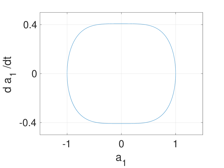
Figure 1: Goldstone periodic orbit for $N=3$, $a_{1}(0)=1$ and $\dot{a}_{1}(0)=0$.

The variational equations (12) can be written for the Goldstone periodic orbit as

$$\ddot{z}_{k}=-\left(\omega_{k}^{2}+{3\over N}\gamma^{2}\mathrm{cn}^{2}(\gamma t,{1\over\sqrt{2}})\right)z_{k},~{}~{}~{}k\in\left\{1,\dots,N\right\}.$$ (19)

Equations (19) are uncoupled Lamé equations in the Jacobian form Ince and can be studied separately for each $k$. Note that the stability domain of (19) was determined for example in Frolov ; it can be seen that there are instable bounds in the plane $(\gamma^{2},\omega_{k}^{2})$.

VI.2 The bivalent periodic orbit

The bivalent periodic orbit $a_{j}(t)$ solution of (17) can be expressed via Jacobi elliptic cosine Abramowitz

$$a_{j}(t)=\gamma\mathrm{cn}(\Omega t,k^{2}),$$

where $\gamma=a_{j}(0),~{}\dot{a}_{j}(0)=0$ and $\Omega^{2}={\omega_{j}^{2}\over 1-2k^{2}},$ while the modulus $k$ of the elliptic function is determined by $2k^{2}={\gamma^{2}\over N\omega_{j}^{2}+\gamma^{2}}.$

For the bivalent periodic orbit, the variational system are uncoupled Lamé equations in the Jacobian form

$$\ddot{z}_{k}=-\left(\omega_{k}^{2}+{3\over N}\gamma^{2}\mathrm{cn}^{2}(\Omega t,k^{2})\right)z_{k},~{}~{}~{}k\in\left\{1,\dots,N\right\}.$$ (20)

For chains, we studied systematically the Floquet multipliers for the Goldstone and the bivalent periodic orbits.

VI.3 Floquet analysis of Goldstone periodic orbit in chains

For chains with $N$ nodes, the instability region of the Goldstone mode is shown in Fig. 2 as a function of the amplitude $a_{1}(0)$. The points indicate instablility. The plot shows the unstable tongues typical of the Mathieu or Lamé equations Frolov . For small chain sizes, there are just a few very narrow unstable tongues, for example for $N=4$, we have three tongues. As the chain gets longer, the number of the unstable tongues and their width increases. Note however that for large enough amplitude, the Goldstone mode is always stable.

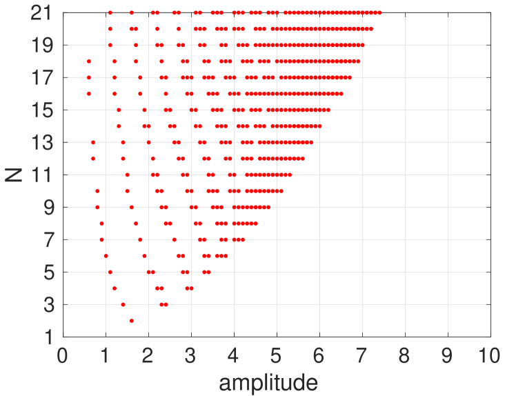
Figure 2: Instability regions of the Goldstone periodic orbit for chains with $N$ nodes for different initial amplitude $a_{1}(0)$.

VI.4 Floquet analysis of the bivalent periodic orbit in chains

Remember that the bivalent mode only exists for chains with an even number of nodes $N$. We calculate the instability region of the bivalent mode $\mathbf{v}^{{N\over 2}+1}$ and present it in Fig. 3 as a function of the amplitude $a_{{N\over 2}+1}(0)$. The points indicate the unstable solutions of (20) with $N$ even. For a narrow region starting from a zero amplitude, the bivalent mode is stable. Above a critical amplitude it is unstable. Notice the difference with the Goldstone mode which is mostly stable while the bivalent mode is mostly unstable.

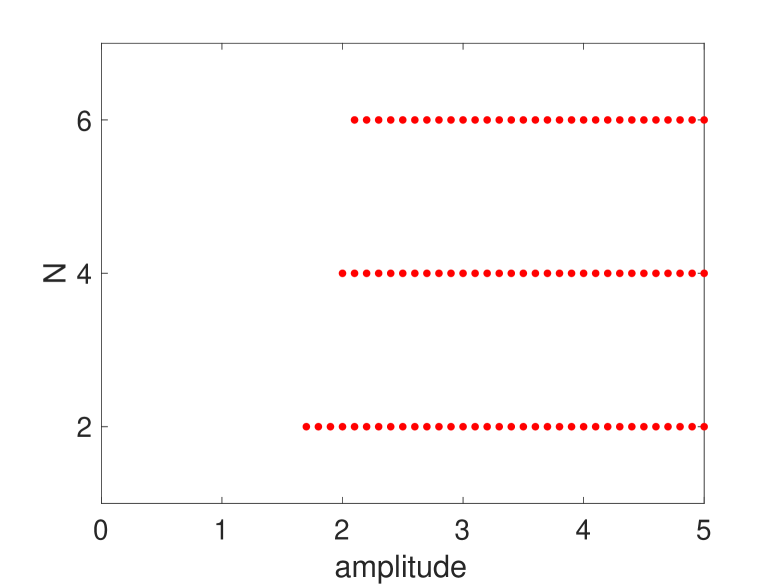
Figure 3: Instability regions of the bivalent mode $\mathbf{v}^{{N\over 2}+1}$ for chains with an even number of nodes $N$ for different amplitudes $a_{{N\over 2}+1}(0)$.

To illustrate the dynamics of the Goldstone and the bivalent modes, we solve (1) for a chain of length 1. We confirm the results of the Floquet analysis and show the couplings that occur in the instability regions.

VI.5 Example: Chain of length 1

For a chain of length 1,

the spectrum is

$$\begin{array}[]{l c r}\omega_{1}^{2}=0,~{}\mathbf{v}^{1}={1\over\sqrt{2}}(1,1)^{T},\\ \\ \omega_{2}^{2}=2,~{}\mathbf{v}^{2}={1\over\sqrt{2}}(1,-1)^{T}.\end{array}$$

The amplitude equations (4) are:

$$\left\{\begin{array}[]{r c l}\ddot{a}_{1}&=&\frac{-1}{2}a_{1}^{3}-{3\over 2}a_{1}a_{2}^{2},\\ \\ \ddot{a}_{2}&=&-2a_{2}-\frac{1}{2}a_{2}^{3}-{3\over 2}a_{1}^{2}a_{2}.\end{array}\right.$$ (21)

First we consider the evolution of the Goldstone nonlinear periodic orbit. We solve numerically (1) for an initial condition $\mathbf{u}(0)=a_{1}(0)\mathbf{v}^{1}$ with $\dot{\mathbf{u}}(0)=0$. The top panel of Fig. 4 shows the amplitudes $a_{1}(t),a_{2}(t)$ for $a_{1}(0)=1.6$. As expected from the Floquet analysis Fig. 2 the orbit is unstable and gives rise to a coupling with the mode $\mathbf{v}^{2}$. On the other hand, for $a_{2}(0)=2$ the amplitudes shown in the bottom panel of Fig. 4 do no show any coupling. The Goldstone mode is stable as shown in Fig. 2.

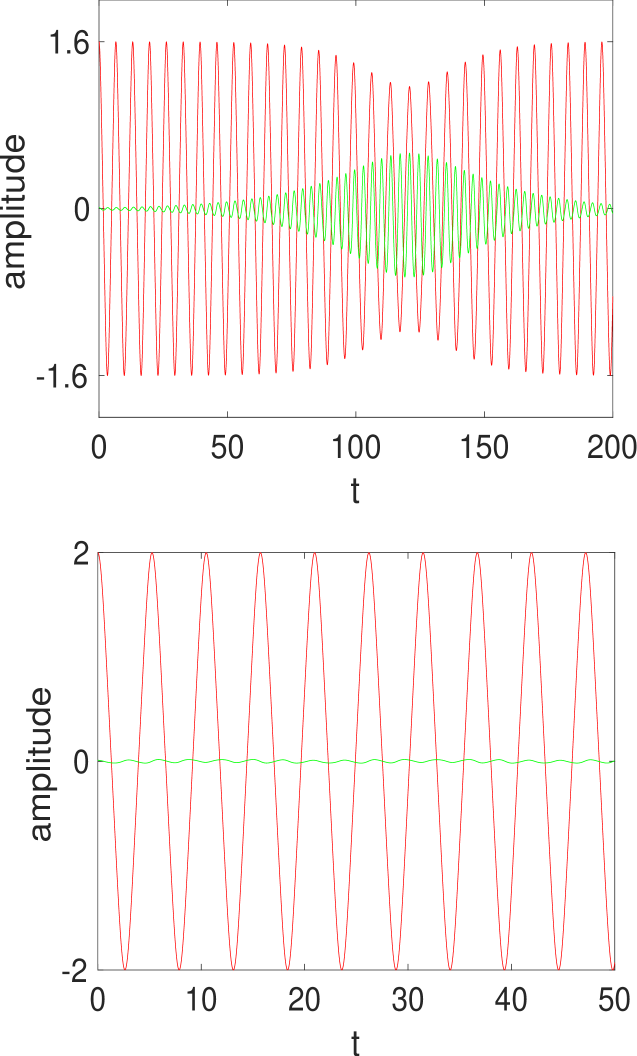
Figure 4: Time evolution of the mode amplitudes $a_{1}$ (red online) and $a_{2}$ (green online) when exciting Goldstone mode $\mathbf{v}^{1}$ for $a_{1}(0)=1.6$ (top) and $a_{1}(0)=2$ (bottom) with $a_{2}(0)=10^{-2}$.

We then consider the evolution of the bivalent mode $\mathbf{v}^{2}$. For that, we solve numerically (1) for an initial condition $\mathbf{u}(0)=a_{2}(0)\mathbf{v}^{2}$ and $\dot{a}_{2}(0)=0$. For $a_{2}(0)=1.5$, the amplitudes shown in the top panel of Fig. 5 do no show any coupling. As expected from the Floquet analysis in Fig. 3, the bivalent mode is stable for $a_{2}(0)<1.7$ and unstable for $a_{2}(0)\geq 1.7$. For $a_{2}(0)=1.7$, we observe coupling to the Goldstone mode as shown in the bottom panel of Fig. 5.

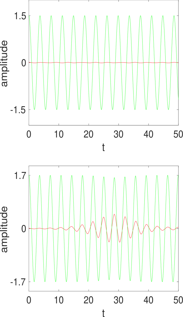
Figure 5: Time evolution of the mode amplitudes $a_{1}$ (red online) and $a_{2}$ (green online) when exciting the bivalent mode $\mathbf{v}^{2}$ for $a_{2}(0)=1.5$ (top) and $a_{2}(0)=1.7$ (bottom) with $a_{1}(0)=10^{-2}$.

VII Nonlinear modes containing soft nodes : Numerical simulations

To illustrate the dynamics of trivalent modes, we consider three examples. These are the single frequency mode in a chain of length 2, the double frequency mode of cycle 3, and the modes of the Network 20 (classification of Cvetkovic1 ). The latter are the single frequency mode and two double frequency modes. We show the difference in the stability of a single frequency mode versus a double frequency mode.

VII.1 chain of length 2

For a chain of length 2,

the spectrum is

$$\begin{array}[]{l c r}\omega_{1}^{2}=0,~{}\mathbf{v}^{1}={1\over\sqrt{3}}(1,1,1)^{T},\\ \\ \omega_{2}^{2}=1,~{}\mathbf{v}^{2}={1\over\sqrt{2}}(1,0,-1)^{T},\\ \\ \omega_{3}^{2}=3,~{}\mathbf{v}^{3}={1\over\sqrt{6}}(1,-2,1)^{T}.\end{array}$$

The amplitude equations (4) are:

$$\left\{\begin{array}[]{l c r}\ddot{a}_{1}=\frac{-1}{3}a_{1}^{3}-a_{1}\left(a_{2}^{2}+a_{3}^{2}\right)+\frac{1}{\sqrt{18}}a_{3}^{3}-\frac{1}{\sqrt{2}}a_{2}^{2}a_{3},\\ \\ \ddot{a}_{2}+a_{2}=\frac{-1}{2}a_{2}^{3}-a_{2}\left(a_{1}^{2}+\frac{1}{2}a_{3}^{2}\right)-\sqrt{2}a_{1}a_{2}a_{3},\\ \\ \ddot{a}_{3}+3a_{3}=\frac{-1}{2}a_{3}^{3}-a_{3}\left(a_{1}^{2}+\frac{1}{2}a_{2}^{2}\right)-\frac{1}{\sqrt{2}}a_{1}a_{2}^{2}+\frac{1}{\sqrt{2}}a_{1}a_{3}^{2}.\end{array}\right.$$ (22)

When exciting the nonlinear mode $\mathbf{v}^{2}$ containing a soft node, with $a_{2}(0)=2$, the modes $\mathbf{v}^{1}$ and $\mathbf{v}^{3}$ will be excited as shown in the top panel of Fig. 6. This instability is explained by two factors. First the coupling terms in the linearized equation (16) do not vanish and the variational system is

$${\mathrm{d}^{2}\over\mathrm{d}t^{2}}\begin{pmatrix}z_{1}\\ z_{2}\\ z_{3}\end{pmatrix}=\begin{pmatrix}-a_{2}^{2}&0&-{1\over 2}a_{2}^{2}\\ 0&-\left(1+{3\over 2}a_{2}^{2}\right)&0\\ -{1\over 2}a_{2}^{2}&0&-\left(3+{1\over 2}a_{2}^{2}\right)\end{pmatrix}\begin{pmatrix}z_{1}\\ z_{2}\\ z_{3}\end{pmatrix}.$$ (23)

The second factor is the closeness of the nonlinear frequency $\omega_{NL}\approx 1.569$ (for $a_{2}(0)=2$) to the linear frequencies of the graph. When the nonlinear frequency is far from the natural frequencies, for example when $a_{2}(0)\geq 3.12$ ($\omega_{NL}\geq 2.128$) the periodic orbit $\mathbf{v}^{2}$ is stable and no coupling with the other modes occurs as shown in the bottom panel of Fig. 6.

Notice that the matrix in the variational equations (23) is the Jacobian matrix Meiss of the system (22) calculated at the periodic orbit $a_{2}$ solution of $\ddot{a}_{2}+a_{2}=\frac{-1}{2}a_{2}^{3}$.

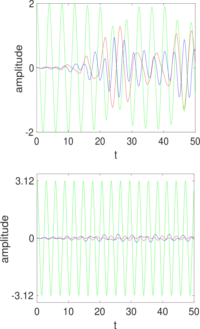
Figure 6: Time evolution of the mode amplitudes $a_{1}$ (red online), $a_{2}$ (green online) and $a_{3}$ (blue online) when exciting the mode $\mathbf{v}^{2}$ with $a_{2}(0)=2$ (top) and $a_{2}(0)=3.12$ (bottom). The other initial amplitudes are $a_{1}(0)=a_{3}(0)=10^{-2}$.

VII.2 Cycle 3

For a cycle 3,

the spectrum is

$$\begin{array}[]{l c r}\omega_{1}^{2}=0,~{}\mathbf{v}^{1}={1\over\sqrt{3}}(1,1,1)^{T},\\ \\ \omega_{2}^{2}=3,~{}\mathbf{v}^{2}={1\over\sqrt{6}}(2,-1,-1)^{T},\\ \\ \omega_{3}^{2}=3,~{}\mathbf{v}^{3}={1\over\sqrt{2}}(0,1,-1)^{T}.\end{array}$$

The amplitude equations (4) are:

$$\begin{array}[]{l c r}\ddot{a}_{1}=\frac{-1}{3}a_{1}^{3}-a_{1}a_{2}^{2}-a_{1}a_{3}^{2}-\frac{1}{\sqrt{18}}a_{2}^{3}+{1\over\sqrt{2}}a_{2}a_{3}^{2},\\ \\ \ddot{a}_{2}+3a_{2}=-a_{1}^{2}a_{2}-{1\over 2}a_{2}^{3}-{1\over 2}a_{2}a_{3}^{2}-{1\over\sqrt{2}}a_{1}a_{2}^{2}+{1\over\sqrt{2}}a_{1}a_{3}^{2},\\ \\ \ddot{a}_{3}+3a_{3}=-a_{1}^{2}a_{3}-{1\over 2}a_{3}^{3}-{1\over 2}a_{2}^{2}a_{3}+\sqrt{2}a_{1}a_{2}a_{3}.\end{array}$$

The nonlinear mode $\mathbf{v}^{3}$ containing a soft node and corresponding to a double frequency, is unstable for all initial amplitudes $a_{3}(0)$. It couples with the modes $\mathbf{v}^{1}$ and $\mathbf{v}^{2}$ as shown in Fig. 7. There, we show the evolution of the amplitudes for initial conditions $a_{3}(0)=2$ (top) and $a_{3}(0)=8$ (bottom). The coupling can be seen in the linearized equations (16)

$${\mathrm{d}^{2}\over\mathrm{d}t^{2}}\begin{pmatrix}z_{1}\\ z_{2}\\ z_{3}\end{pmatrix}=\begin{pmatrix}-a_{3}^{2}&{1\over\sqrt{2}}a_{3}^{2}&0\\ {1\over\sqrt{2}}a_{3}^{2}&-\left(3+{1\over 2}a_{3}^{2}\right)&0\\ 0&0&-\left(3+{3\over 2}a_{3}^{2}\right)\end{pmatrix}\begin{pmatrix}z_{1}\\ z_{2}\\ z_{3}\end{pmatrix}.$$

The instability observed for large initial amplitudes seems to be due to the degeneracy of the linear frequency as we discuss below.

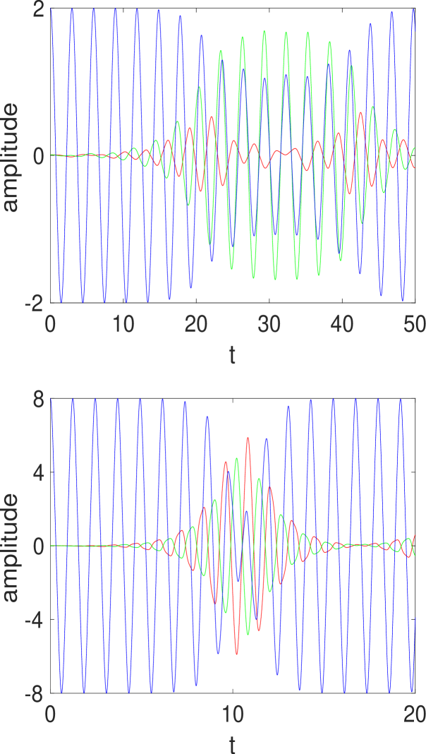
Figure 7: Time evolution of the mode amplitudes $a_{1}$ (red online), $a_{2}$ (green online) and $a_{3}$ (blue online) when exciting the mode $\mathbf{v}^{3}$ for $a_{3}(0)=2$ (top) and $a_{3}(0)=8$ (bottom) with $a_{1}(0)=a_{2}(0)=10^{-2}$.

VII.3 Network 20

Network 20 contain nonlinear mode with soft node corresponding to a simple frequency, and two nonlinear modes with soft nodes corresponding to a double frequency. The spectrum is

$$\begin{array}[]{l c r}\omega_{1}=0,~{}\mathbf{v}^{1}={1\over\sqrt{5}}(1,1,1,1,1)^{T},\\ \\ \omega_{2}^{2}=1,~{}\mathbf{v}^{2}={1\over 2}(1,1,0,-1,-1)^{T},\\ \\ \omega_{3}^{2}=3,~{}\mathbf{v}^{3}={1\over\sqrt{2}}(-1,1,0,0,0)^{T},\\ \\ \omega_{4}^{2}=3,~{}\mathbf{v}^{4}={1\over\sqrt{2}}(0,0,0,-1,1)^{T},\\ \\ \omega_{5}^{2}=5,~{}\mathbf{v}^{5}={1\over\sqrt{20}}(-1,-1,4,-1,-1)^{T}.\end{array}$$

When exciting the nonlinear mode $\mathbf{v}^{2}$ containing a soft node and corresponding to a simple frequency $\omega_{2}=1$ for initial conditions $2.3\leq a_{2}(0)\leq 3.37$, there is coupling with the modes $\mathbf{v}^{1}$ and $\mathbf{v}^{5}$ as shown in Table 1. There is no coupling with $\mathbf{v}^{3}$ and $\mathbf{v}^{4}$ since the soft node $3$ for $\mathbf{v}^{2}$ is also soft for the modes $\mathbf{v}^{3}$ and $\mathbf{v}^{4}$, so that the coupling terms vanish in (16). For $a_{2}(0)\geq 3.38$ ($\omega_{NL}\geq 1.755$), the nonlinear mode $\mathbf{v}^{2}$ is stable; there is no coupling with the other modes.

The nonlinear modes $\mathbf{v}^{3}$ and $\mathbf{v}^{4}$ have soft nodes and correspond to the double frequency $\omega_{3}=\omega_{4}=\sqrt{3}$. When exciting $\mathbf{v}^{3}$ with a small amplitude $a_{3}(0)<1.5$ we see no coupling with the other modes. Starting from $a_{3}(0)\geq 1.5$ ($\omega_{NL}\geq 1.9587$) there is coupling with the modes $\mathbf{v}_{1},~{}\mathbf{v}_{2}$ and $\mathbf{v}_{5}$ as shown in Table 1 and no coupling with $\mathbf{v}^{4}$. This is because the coupling terms in (16) corresponding to the mode $\mathbf{v}^{4}$ vanish, $\sum_{m\in\mathcal{S}_{3}}v_{m}^{4}v_{m}^{k}=0,~{}~{}\forall~{}k\neq 4$ where $\mathcal{S}_{3}$ is the set of the soft nodes of the nonlinear mode $\mathbf{v}^{3}$. We observe similar effects when exciting $\mathbf{v}^{4}$ instead of $\mathbf{v}^{3}$, see Table 1.

Excited modes	$\omega_{j}$	Nonlinear frequency	amplitude for instability	Activated modes
$\mathbf{v}_{2}$	$1$	$[1.404,1.751]$	$[2.3,3.37]$	$\mathbf{v}_{2},~{}\mathbf{v}_{1},~{}\mathbf{v}_{5}$
$\mathbf{v}_{3}$	$\sqrt{3}$	$\geq 1.958$	$\geq 1.5$	$\mathbf{v}_{3},~{}\mathbf{v}_{1},~{}\mathbf{v}_{2},~{}\mathbf{v}_{5}$
$\mathbf{v}_{4}$	$\sqrt{3}$	$\geq 1.958$	$\geq 1.5$	$\mathbf{v}_{4},~{}\mathbf{v}_{1},~{}\mathbf{v}_{2},~{}\mathbf{v}_{5}$

Table 1: Excited modes and their associated linear frequencies, nonlinear frequencies depending on the initial amplitudes for instability region, and the activated modes.

To summarize, we observe that a trivalent periodic orbit is stable for large amplitudes when the eigenvalue is simple. Conversely, when the eigenvalue is double, the periodic orbit is unstable. In fact, the criterion of Aoki aoki is realized only for a particular choice of eigenvectors. Rotating the eigenspace will break the criterion and destroy the periodic orbits. In that sense, a trivalent periodic orbit for a multiple eigenvalue is structurally unstable.

VIII Conclusions

The graph wave equation arises naturally from conservation laws on a network. There, the usual continuum Laplacian is replaced by the graph Laplacian. We consider such a wave equation with a cubic non-linearity on a general network. We identified a criterion allowing to extend some linear normal modes of the graph Laplacian into nonlinear periodic orbits. Three different types of periodic orbits were found, the monovalent, bivalent and trivalent ones depending whether they contain $1$ or $-1,+1$ or $-1,0,+1$. For the monovalent and bivalent modes, the linearized equations decouple into $N$ Hill-like equations. For chains, the monovalent mode is mostly stable while the bivalent is unstable.

Trivalent modes contain soft nodes and the variational equations do not decouple. The stability is governed by a system of coupled resonance equations; they indicate which modes will be excited when the orbit is unstable. Modes that share a soft node with a trivalent orbit will not be excited. Numerical results show that trivalent modes with a single eigenvalue are unstable below a treshold amplitude. Conversely, trivalent modes with multiple eigenvalues seem always unstable.

This study can be applied to complex physical networks, like coupled mechanical systems.

Appendix A Spectrum of cycles and chains

Spectrum of cycles

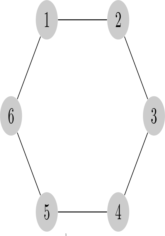
Figure 8: Cycle 6

For cycles, the Laplacian $\mathbf{\Delta}$ in (1) is a circulant matrix Cvetkovic2 where each row vector is rotated one element to the right relative to the preceding row vector.

$$\mathbf{\Delta}=\begin{pmatrix}-2&1&0&\dots&0&1\\ 1&-2&1&0&\dots&0\\ 0&\ddots&\ddots&\ddots&\ddots&\vdots\\ \vdots&\ddots&\ddots&\ddots&\ddots&0\\ 0&\dots&0&1&-2&1\\ 1&0&\dots&0&1&-2\end{pmatrix}$$

The repeated eigenvalues are

$$\begin{array}[]{l c r}-\omega_{2k}^{2}=-\omega_{2k+1}^{2}=-4\sin^{2}\left(\frac{k\pi}{N}\right),\end{array}$$

for $k=1,\dots,\frac{N-1}{2}$ (resp. $k=1,\dots,\frac{N-2}{2}$) if $N$ is odd (resp. $N$ is even). The first eigenvalue $-\omega_{1}^{2}=0$ is simple. When $N$ is even, the last one $-\omega_{N}^{2}=-4$ is also simple. The components of Goldstone eigenvector $v_{m}^{1}=\frac{1}{\sqrt{N}},~{}m\in\{1,...,N\}$. We present in the following the components of the corresponding orthonormal eigenvectors for $j\in\left\{2,\dots,N\right\}$

$$v_{m}^{j}=\left\{\begin{array}[]{l c r}\sqrt{2\over N}\cos\left(\frac{j\pi}{N}(m-1)\right),m\in\left\{1,\dots,N\right\},~{}j\text{ even},\\ \\ \sqrt{2\over N}\sin\left(\frac{(j-1)\pi}{N}(m-1)\right),m\in\left\{1,\dots,N\right\},~{}j\text{ odd}.\end{array}\right.$$

Spectrum of chains

Figure 9: Chain of length 3

For a chain of length $N-1$ (with $N$ nodes), the Laplacian matrix is

$$\mathbf{\Delta}=\begin{pmatrix}-1&1&0&\dots&0\\ 1&-2&1&\ddots&\vdots\\ 0&\ddots&\ddots&\ddots&0\\ \vdots&\ddots&1&-2&1\\ 0&\dots&0&1&-1\end{pmatrix}$$

The spectrum of $\mathbf{\Delta}$ is well known Edwards . The eigenvalues are simple:

$$-\omega_{j}^{2}=-4\sin^{2}\left(\frac{(j-1)\pi}{2N}\right),\ j\in\{1,...,N\}.$$

The corresponding eigenvectors have components

$$v^{j}_{m}=\sqrt{2\over N}\cos\left(\frac{(j-1)\pi}{N}(m-\frac{1}{2})\right),~{}~{}~{}j,m\in\{1,...,N\}.$$

Appendix B Existence of 2-mode solutions

We seek nonlinear solutions of (1) that involve two nonlinear normal modes. Substituting the ansatz,

$$\mathbf{u}(t)=a_{j}(t)\mathbf{v}^{j}+a_{k}(t)\mathbf{v}^{k},$$ (24)

into the equation of motion (1) and projecting on each mode $\mathbf{v}^{j}$ and $\mathbf{v}^{k}$, we get

$$\left\{\begin{array}[]{r c l}\ddot{a}_{j}=-\omega_{j}^{2}a_{j}-\sum_{m=1}^{N}u_{m}^{3}v_{m}^{j},\\ \\ \ddot{a}_{k}=-\omega_{k}^{2}a_{k}-\sum_{m=1}^{N}u_{m}^{3}v_{m}^{k},\end{array}\right.$$

where we have used the orthogonality of the eigenvectors $\left\langle\mathbf{v}^{j},\mathbf{v}^{k}\right\rangle=0$. The term $u_{m}^{3}$ can be written as

$$u_{m}^{3}=a_{j}^{3}(v_{m}^{j})^{3}+3a_{j}^{2}a_{k}(v_{m}^{j})^{2}v_{m}^{k}+3a_{j}a_{k}^{2}v_{m}^{j}(v_{m}^{k})^{2}+a_{k}^{3}(v_{m}^{k})^{3},$$

so that the above equations can be written

$$\ddot{a}_{j}=-\omega_{j}^{2}a_{j}-a_{j}^{3}\sum_{{m=1}}^{N}(v_{m}^{j})^{4}-3a_{j}^{2}a_{k}\sum_{{m=1}}^{N}(v_{m}^{j})^{3}v_{m}^{k}$$

$$-3a_{j}a_{k}^{2}\sum_{{m=1}}^{N}(v_{m}^{j})^{2}(v_{m}^{k})^{2}-a_{k}^{3}\sum_{{m=1}}^{N}(v_{m}^{k})^{3}v_{m}^{j},$$

$$\ddot{a}_{k}=-\omega_{k}^{2}a_{k}-a_{k}^{3}\sum_{{m=1}}^{N}(v_{m}^{k})^{4}-3a_{j}^{2}a_{k}\sum_{{m=1}}^{N}(v_{m}^{j})^{2}(v_{m}^{k})^{2}$$

$$-3a_{j}a_{k}^{2}\sum_{{m=1}}^{N}v_{m}^{j}(v_{m}^{k})^{3}-a_{j}^{3}\sum_{{m=1}}^{N}(v_{m}^{j})^{3}v_{m}^{k}.$$

To have two periodic solutions for $a_{j}$ and $a_{k}$, these equations should be uncoupled and this imposes

$$\sum_{{m=1}}^{N}(v_{m}^{j})^{3}v_{m}^{k}=0,~{}~{}\sum_{{m=1}}^{N}(v_{m}^{j})^{2}(v_{m}^{k})^{2}=0,~{}~{}\sum_{{m=1}}^{N}v_{m}^{j}(v_{m}^{k})^{3}=0,$$ (25)

in which case the equations reduce to

$$\left\{\begin{array}[]{l c r}\ddot{a}_{j}=-\omega_{j}^{2}a_{j}-{1\over N-S_{j}}a_{j}^{3},\\ \\ \ddot{a}_{k}=-\omega_{k}^{2}a_{k}-{1\over N-S_{k}}a_{k}^{3}.\end{array}\right.$$

where $S_{j}$ is the number of soft nodes of $\mathbf{v}^{j}$ and $S_{k}$ is the number of soft nodes of $\mathbf{v}^{k}$.

The condition (25) is the criteria for the existence of $2$-mode solutions. It is clear that not all nonlinear modes satisfy this condition. From the examples mentioned in section IV, only cycles where $N$ is multiple of $4$ exhibit nonlinear normal modes satisfying the condition (25), they are the nonlinear modes $\mathbf{v}^{N\over 2}$ and $\mathbf{v}^{{N\over 2}+1}$ corresponding to the double frequency $\omega_{N\over 2}=\omega_{{N\over 2}+1}=\sqrt{2}$.

References

- (1) L. D. Landau and E. M. Lifchitz, Mechanics, Volume 1 of Course of Theoritical Physics. 3rd ed. (Pergamon, Oxford, 1976).
- (2) E. Fermi, J. Pasta, and S. Ulam, Collected Papers of Enrico Fermi, (University of Chicago Press, Chicago, 1965).
- (3) S. Flach and C. R Willis, Discrete breathers. Physics reports 295, 181-264 (1998).
- (4) S. Flach and A. V. Gorbach, Discrete breathers - Advances in theory and applications. Physics Reports 467, 1-116 (2008).
- (5) P. Panayotaros, Continuation of normal modes in finite NLS lattices , Physics Letters A 374, 3912–3919 (2010).
- (6) G. M. Chechin, G. M. Ryabov, and K. G. Zhukov, Stability of low-dimensional bushes of vibrational modes in the Fermi-Pasta-Ulam chains Physics D 203, 121 (2005).
- (7) T. Bountis, G. Chechin, and V. Sakhnenko, Discrete symmetry and stability in Hamiltonian dynamics. Int. J. Bif. Chaos 21, 1539 (2011).
- (8) G. M. Chechin and D. S. Ryabov, Stability of nonlinear normal modes in the Fermi-Pasta-Ulam chain in the thermodynamic limit. Phys. Rev. E 85, 056601 (2012).
- (9) K. V. Avramov, Y. V.Mikhlin. Review of Applications of Nonlinear Normal Modes for Vibrating Mechanical Systems. Applied Mechanics Reviews 65, 020801, American Society of Mechanical Engineers (2013).
- (10) Kenichiro Aoki, Stable and unstable periodic orbits in the one-dimensional lattice theory. Phys. Rev. E 94, 042209 (2016).
- (11) J.-G. Caputo, A. Knippel and E. Simo, Oscillations of networks: the role of soft nodes. J. Phys. A: Math. Theor. 46 035101 (2013).
- (12) D. Cvetkovic, P. Rowlinson and S. Simic, An Introduction to the Theory of Graph Spectra. London Mathematical Society Student Texts (No. 75) (2001).
- (13) A. C. Scott, Nonlinear Science: Emergence and Dynamics of Coherent Structures. Oxford Texts in Applied and Engineering Mathematics (1999).
- (14) W. Strauss, Nonlinear invariant wave equations. Lecture notes in physics, G. Velo and A. Wightman, Springer (1978).
- (15) A. C. Scott, Encyclopedia of nonlinear science. Ed., Routledge (Taylor and Francis) (2005).
- (16) J.-G. Caputo and A. Knippel, Classification of -soft graphs, in preparation.
- (17) James D. Meiss, Differential Dynamical Systems. SIAM (2007).
- (18) The Mathworks, www.mathworks.com
- (19) Abramowitz, M. and Stegun, I. Handbook of Mathematical Functions, Dover (1965).
- (20) E. L. Ince, Ordinary differential equations. New York, Dover Publications (1956).
- (21) Andrei V. Frolov, Non-linear Dynamics and Primordial Curvature Perturbations from Preheating. Classical and Quantum Gravity 27(12):124006 (2010).
- (22) R. A. Brualdi, D. Cvetkovic, A Combinatorial Approach to Matrix Theory and Its Applications. Discrete Mathematics and Its Applications (2008).
- (23) T. Edwards, The Discrete Laplacian of a Rectangular Grid, web document (2013). https://www.math.washington.edu/~reu/papers/2013/tom/DiscreteLaplacianofRectangularGrid.pdf