Improving the Betweenness Centrality of a Node by Adding Links

Abstract.

Betweenness is a well-known centrality measure that ranks the nodes according to their participation in the shortest paths of a network. In several scenarios, having a high betweenness can have a positive impact on the node itself. Hence, in this paper we consider the problem of determining how much a vertex can increase its centrality by creating a limited amount of new edges incident to it. In particular, we study the problem of maximizing the betweenness score of a given node – Maximum Betweenness Improvement (MBI) – and that of maximizing the ranking of a given node – Maximum Ranking Improvement (MRI). We show that MBI cannot be approximated in polynomial-time within a factor $(1-\frac{1}{2e})$ and that MRI does not admit any polynomial-time constant factor approximation algorithm, both unless $P=NP$. We then propose a simple greedy approximation algorithm for MBI with an almost tight approximation ratio and we test its performance on several real-world networks. We experimentally show that our algorithm highly increases both the betweenness score and the ranking of a given node and that it outperforms several competitive baselines. To speed up the computation of our greedy algorithm, we also propose a new dynamic algorithm for updating the betweenness of one node after an edge insertion, which might be of independent interest. Using the dynamic algorithm, we are now able to compute an approximation of MBI on networks with up to $10^{5}$ edges in most cases in a matter of seconds or a few minutes.

1. Introduction

In recent years, the analysis of complex networks has become an extremely active research area. One of the main tasks in network analysis is computing the ranking of nodes based on their structural importance. Since the notion of importance can vary significantly depending on the application, several centrality measures have been introduced in the literature. One of the most popular measures is betweenness centrality, which ranks the nodes according to their participation in the shortest paths between other node pairs. Intuitively, betweenness measures a node’s influence on the flow circulating through the network, under the assumption that the flow follows shortest paths.

Computing betweenness centrality in unweighted graphs requires $\Theta(nm)$ time with Brandes’s algorithm (Brandes, 2001), where $n$ is the number of nodes and $m$ is the number of edges. Since this can be prohibitive for very large networks, several approximation algorithms exist in the literature (Borassi and Natale, 2016; Geisberger et al., 2008; Riondato and Upfal, 2016; Riondato and Kornaropoulos, 2016). Also for dynamic networks that evolve over time, such as social networks and the Web graph, recomputing betweenness at every time step can be too expensive. For this reason, a variety of dynamic algorithms have been proposed over the last years (Green et al., 2012; Kas et al., 2013; Lee et al., 2016; Nasre et al., 2014; Pontecorvi and Ramachandran, 2015; Bergamini et al., 2017). These algorithms usually keep track of the betweenness scores and additional information, such as the pairwise distances, and update them accordingly after a modification in the graph. Another problem that has recently been considered for betweenness and other centrality measures is the quick identification of the $k$ most central nodes without computing the score of each node (Bergamini et al., 2016; Lee and Chung, 2014).

There are several contexts in which having a high betweenness can be beneficial for the node itself. For example, in the field of transportation network analysis, the betweenness centrality seems to be positively related to the efficiency of an airport (see (Malighetti et al., 2009), where a network of 57 European airports has been analyzed). Also, increasing the betweenness of an airport would mean more traffic flowing through it and possibly more customers for its shops. In the context of social networks, Valente and Fujimoto (Valente and Fujimoto, 2010) claim that brokers (or “bridging individuals”) “may be more effective at changing others, more open to change themselves, and intrinsically interesting to identify”. In (Everett and Valente, 2016), the authors show that a slightly modified version of betweenness centrality can be used to find brokers. Also, the authors of (Mahmoody et al., 2016) show experimentally that nodes with high betweenness are also very effective in spreading influence to other nodes in a social network. Therefore, it might be interesting for a user to create new links with other users or pages in order to increase his own influence spread.

The problem of increasing the centrality of a node has attracted considerable attention for page-rank (Avrachenkov and Litvak, 2006; Olsen and Viglas, 2014), where much effort has been devoted to “fooling” search engines in order to increase the popularity of some web pages (an example is the well-known link farming (Wu and Davison, 2005)). In addition to page-rank, the problem has been considered also for other centrality measures, such as closeness centrality (Crescenzi et al., 2016) and eccentricity (Demaine and Zadimoghaddam, 2010; Perumal et al., 2013).

In the above mentioned contexts, it is reasonable to assume that, in order to increase its betweenness, a node can only add edges incident to itself. Hence, in this paper we address the following problem: assuming that a node $v$ can connect itself with $k$ other nodes, how can we choose these nodes in order to maximize the betweenness centrality of $v$? In other terms we want to add a set of $k$ edges to the graph (all incident to $v$), such that the betweenness of $v$ in the new graph is as high as possible. For directed graphs, we assume the edges we want to add are of the form $(w,v)$ (i.e. incoming edges). However, our results apply also to the problem where $k$ outgoing edges need to be added. Indeed, in our proofs, we could simply use $G$ transposed instead of $G$, and the results would also be valid in the case where we want to add outgoing edges.

Since in some contexts one might be more interested in having a high ranking among other nodes rather than a high betweenness score, we also consider the case where we want to maximize the ranking increment of a node instead of its betweenness. We call such two optimization problems maximum betweenness improvement (MBI) and maximum ranking improvement (MRI), respectively.

Our contribution

We study both MBI and MRI problems in directed graphs. Our contribution can be summarized as follows: $(i)$ We provide two hardness results, one for MBI and one for MRI. In particular, we prove that, unless $P=NP$, MBI cannot be approximated within a factor greater than $1-\frac{1}{2e}$. Also, we show that, for any constant $\alpha\leq 1$, there is no $\alpha-$approximation algorithm for MRI, unless $P=NP$ (Section 4). $(ii)$ We propose a greedy algorithm for MBI, which yields a $(1-\frac{1}{e})-$approximation (Section 5). This is in contrast with the results for the undirected graph case, where it is known that the same algorithm has an unbounded approximation ratio (D’Angelo et al., 2016). The complexity of the algorithm, if implemented naively, is $O(kn^{2}m)$. $(iii)$ To make our greedy approach faster, we also develop a new algorithm for recomputing the betweenness centrality of a single node after an edge insertion or a weight decrease (Section 6). The algorithm, which might be of independent interest, builds on a recent method for updating the betweenness of all nodes (Bergamini et al., 2017). In the worst case, our algorithm updates the betweenness of one node in $O(n^{2})$ time, whereas all existing dynamic algorithms have a worst-case complexity of at least $\Theta(nm)$. This is in contrast with the static case, where computing betweenness of all nodes is just as expensive as computing it for one node (at least, no algorithm exists that computes the betweenness of one node faster than for all nodes). In a context where the betweenness centrality of a single node needs to be recomputed, our experimental evaluation (Section 7.2) shows that our new algorithm is much faster than existing algorithms, on average by a factor $18$ for directed and $29$ for undirected graphs (geometric mean of the speedups). Also, using our dynamic algorithm, the worst-case complexity of our greedy approach for MBI decreases to $O(kn^{3})$. However, our experiments show that it is actually much faster in practice. For example, we are able to target directed networks with hundreds of thousands of nodes in a few minutes.

In terms of solution quality, our experiments in Section 7.1 show that on directed random graphs, the approximation ratio (the ratio between the solution found by the optimum and the one found by our greedy algorithm) is never smaller than 0.96 for the instances used. Also, we show that on real-world networks the greedy approach outperforms other heuristics, both in terms of betweenness improvement and ranking improvement. Although the approximation guarantee holds only for directed graphs, our tests show that the greedy algorithm works well also on undirected real-world networks.

2. Related work

Centrality improvement

In the following we describe the literature about algorithms that aim at optimizing some property of a graph by adding a limited number of edges. In (Meyerson and Tagiku, 2009), the authors give a constant factor approximation algorithm for the problem of minimizing the average shortest-path distance between all pairs of nodes. Other works (Papagelis et al., 2011; Parotsidis et al., 2015) propose new algorithms for the same problem and show experimentally that they are good in practice. In (Bauer et al., 2012), the authors study the problem of minimizing the average number of hops in shortest paths of weighted graphs, and prove that the problem cannot be approximated within a logarithmic factor, unless $P=NP$. They also propose two approximation algorithms with non-constant approximation guarantees. (Tong et al., 2012) and (Saha et al., 2015) focus on the problem of maximizing the leading eigenvalue of the adjacency matrix and give algorithms with proven approximation guarantees.

Some algorithms with proven approximation guarantees for the problem of minimizing the diameter of a graph are presented in (Bilò et al., 2012) and (Frati et al., 2015).

In (Li and Yu, 2015) and (Dehghani et al., 2015), the authors propose approximation algorithms with proven guarantees for the problem of making the number of triangles in a graph minimum and maximum, respectively. In (Papagelis, 2015), the author studies the problem of minimizing the characteristic path length.

The problem analyzed in this paper differs from the above mentioned ones as it focuses on improving the centrality of a predefined vertex. Similar problems have been studied for other centrality measures, i.e. page-rank (Avrachenkov and Litvak, 2006; Olsen and Viglas, 2014), eccentricity (Demaine and Zadimoghaddam, 2010; Perumal et al., 2013), average distance (Meyerson and Tagiku, 2009), some measures related to the number of paths passing through a given node (Ishakian et al., 2012), and closeness centrality (Crescenzi et al., 2015, 2016). In particular, in (Crescenzi et al., 2016) the authors study the problem of adding a limited amount of edges incident to a target node in order to increase its harmonic centrality (a variant of closeness). They prove that the problem cannot be approximated within a factor greater than $1-\frac{1}{3e}$ ($1-\frac{1}{15e}$ on undirected graphs) and they design a $1-\frac{1}{e}$-approximation algorithm to solve it. They also make use of heuristics to decrease the computational time and run experiments on large real-world networks. In this work we show how to adapt the greedy algorithm presented in (Crescenzi et al., 2016) according to the definition of betweenness centrality in order to study the MBI problem.

The MBI problem has been studied for undirected weighted graphs (D’Angelo et al., 2016) and it has been proved that, in this case, the problem cannot be approximated within a factor greater than $1-\frac{1}{2e}$, unless $P=NP$. They proved this bound using a technique similar to the one used in (Crescenzi et al., 2015) for the harmonic centrality (and to the one used in this paper for directed graphs). Also, D’Angelo et al. (D’Angelo et al., 2016) show that a natural greedy algorithm exhibits an arbitrarily small approximation ratio. Nevertheless, in their experiments on small networks with up to few hundreds of nodes, they show that the greedy algorithm provides a solution near to the optimal. In this paper, we make the greedy algorithm orders of magnitude faster by combining it with a new dynamic algorithm for updating the betweenness of one node and we study the behavior of the algorithm on directed and undirected networks with up to $10^{4}$ nodes and $10^{5}$ edges.

Dynamic algorithms for betweenness centrality

The general idea of dynamic betweenness algorithms is to keep track of the old betweenness values and to update them after some modification happens to the graph, which might be an edge or node insertion, an edge or node deletion, or a change in an edge’s weight. In particular, in case of edge insertions or weight decreases, the algorithms are often referred to as incremental, whereas for edge deletions or weight increases they are called decremental. All dynamic algorithms existing in the literature update the centralities of all nodes and most of them first update the distances and shortest paths between nodes and then recompute the fraction of shortest paths each node belongs to. The approach proposed by Green et al. (Green et al., 2012) for unweighted graphs maintains all previously calculated betweenness values and additional information, like the distance between each node pair and the list of predecessors, i.e. the nodes immediately preceding $v$ in the shortest paths from $s$ to $v$, for all node pairs $(s,v)$. Using this information, the algorithm limits the recomputation to the nodes whose betweenness has actually been affected. Kourtellis et al. (Kourtellis et al., 2015) modify the approach by Green et al. (Green et al., 2012) in order to reduce the memory requirements from $O(nm)$ to $O(n^{2})$. Instead of storing the predecessors of each node $v$ from each possible source, they recompute them every time the information is required.

Kas et al. (Kas et al., 2013) extend an existing algorithm for the dynamic all-pairs shortest paths (APSP) problem by Ramalingam and Reps (Ramalingam and Reps, 1996) to also update BC scores. Nasre et al. (Nasre et al., 2014) compare the distances between each node pair before and after the update and then recompute the dependencies as in Brandes’s algorithm. Although this algorithm is faster than recomputation on some graph classes (i.e. when only edge insertions are allowed and the graph is sparse and weighted), it was shown in (Bergamini et al., 2015) that its performance in practice is always worse than that of the algorithm proposed in (Green et al., 2012). Pontecorvi and Ramachandran (Pontecorvi and Ramachandran, 2015) extend existing fully-dynamic APSP algorithms with new data structures to update all shortest paths and then recompute dependencies as in Brandes’s algorithm. Differently from the previous algorithms, the approach by Lee et al. (Lee et al., 2016) is not based on dynamic APSP algorithms, but splits the graph into biconnected components and then recomputes the betweenness values from scratch only within the component affected by the graph update. Although this allows for a smaller memory requirement ($\Theta(m)$ versus $\Omega(n^{2})$ needed by the other approaches), the speedups on recomputation reported in (Lee et al., 2016) are significantly worse than those reported for example in (Green et al., 2012) or Kas et al. (Kas et al., 2013).

Very recently, a new approach called iBet for updating betweenness after an edge insertion or a weight decrease has been proposed (Bergamini et al., 2017). The approach improves over the one by Kas et al. (Kas et al., 2013) by removing redundant work in both the APSP update step and the dependency accumulation. In their experiments, the authors show that iBet outperforms existing dynamic algorithms by about one order of magnitude. Since our new dynamic algorithm for updating the betweenness of a single node builds on iBet, we will describe it in more detail in Section 6.1.

Recently, also dynamic algorithms that update an approximation of betweenness centrality have been proposed (Bergamini and Meyerhenke, 2016; Hayashi et al., 2015; Riondato and Upfal, 2016). Notice that all existing dynamic algorithms update the betweenness of all nodes and their worst-case complexity is, in general, the same as static recomputation. This means, for exact algorithms, $O(nm)$ in unweighted and $O(n(m+n\log n))$ in weighted graphs.

3. Notation and problem statement

Let $G=(V,E)$ be a directed graph where $|V|=n$ and $|E|=m$. For each node $v$, $N_{v}$ denotes the set of in-neighbors of $v$, i.e. $N_{v}=\{u~{}|~{}(u,v)\in E\}$. Given two nodes $s$ and $t$, we denote by $d_{st}$, $\sigma_{st}$, and $\sigma_{stv}$ the distance from $s$ to $t$ in $G$, the number of shortest paths from $s$ to $t$ in $G$, and the number of shortest paths from $s$ to $t$ in $G$ that contain $v$, respectively. For each node pair $(s,t$), we assume $d_{st}\geq 0$. For each node $v$, the betweenness centrality (Freeman, 1977) of $v$ is defined as

(1) $$b_{v}=\sum_{\begin{subarray}{c}s,t\in V\\ s\neq t;s,t\neq v\\ \sigma_{st}\neq 0\end{subarray}}\frac{\sigma_{stv}}{\sigma_{st}}.$$

In case $\sigma_{st}=0$, the corresponding term in the sum is defined to be 0. The ranking of each node $v$ according to its betweenness centrality is defined as

(2) $$r_{v}=|\{u\in V~{}|~{}b_{u}>b_{v}\}|+1.$$

In this paper, we consider graphs that are augmented by adding a set $S$ of arcs not in $E$. Given a set $S\subseteq V\times V\setminus E$ of arcs, we denote by $G(S)$ the graph augmented by adding the arcs in $S$ to $G$, i.e. $G(S)=(V,E\cup S)$. For a parameter $x$ of $G$, we denote by $x(S)$ the same parameter in graph $G(S)$, e.g. the distance from $s$ to $t$ in $G(S)$ is denoted as $d_{st}(S)$.

The betweenness centrality of a node might change if the graph is augmented with a set of arcs. In particular, adding arcs incident to some node $v$ can increase the betweenness of $v$ and its ranking. We are interested in finding a set $S$ of arcs incident to a particular node $v$ that maximizes $b_{v}(S)$. Therefore, we define the following optimization problem.

Maximum Betweenness Improvement (MBI)
Given:	A directed graph $G=(V,E)$; a node $v\in V$; an integer $k\in\mathbb{N}$
Solution:	A set $S$ of arcs incident to $v$, $S=\{(u,v)~{}|~{}u\in V\setminus N_{v}\}$, such that $|S|\leq k$
Objective:	Maximize $b_{v}(S)$

Note that maximizing the betweenness value of a node $v$ does not necessarily lead to maximizing the ranking position of $v$. For example, consider the graph in Figure 1: before the addition of the edge $(u,v)$ the initial betweenness values are $b_{u}=2$, $b_{v}=1$ and $b_{a}=b_{b}=b_{c}=b_{d}=b_{e}=0$ while the initial ranking is $r_{u}=1$, $r_{v}=2$ and $r_{a}=r_{b}=r_{c}=r_{d}=r_{e}=0$. After the addition of the edge $(u,v)$ the new betweenness values are $b^{\prime}_{u}=6$, $b^{\prime}_{v}=4$ and $b_{a}=b_{b}=b_{c}=b_{d}=b_{e}=0$ but the ranking remains the same.

Therefore, we also consider the problem of finding a set $S$ of arcs incident to node $v$ that maximizes the increment of the ranking of $v$ with respect to its original ranking. We denote such an increment as $\rho_{v}(S)$, that is,

$$\rho_{v}(S)=r_{v}-r_{v}(S).$$

Informally, $\rho(S)$ represents the number of nodes that $v$ “overtakes” by adding arcs in $S$ to $G$. Therefore, we define the following optimization problem.

Maximum Ranking Improvement (MRI)
Given:	A directed graph $G=(V,E)$; a vertex $v\in V$; and an integer $k\in\mathbb{N}$
Solution:	A set $S$ of arcs incident to $v$, $S=\{(u,v)~{}|~{}u\in V\setminus N(v)\}$, such that $|S|\leq k$
Objective:	Maximize $\rho_{v}(S)$

Figure 1. Graph in which the addition of the edge $(u,v)$ affects the betweenness value but not the ranking.

4. Hardness of approximation

In this section we first show that it is $NP$-hard to approximate problem MBI within a factor greater than $1-\frac{1}{2e}$. Then, we focus on the MRI problem and show that it cannot be approximated within any constant bound, unless $P=NP$.

Theorem 4.1.

Problem MBI cannot be approximated within a factor greater than $1-\frac{1}{2e}$, unless $P=NP$.

Proof.

We give an L-reduction with parameters $a$ and $b$ (Williamson and Shmoys, 2011, Chapter 16) to the maximum set coverage problem (MSC) defined as follows: given a finite set $X$, a finite family $\mathcal{F}$ of subsets of $X$, and an integer $k^{\prime}$, find $\mathcal{F}^{\prime}\subseteq\mathcal{F}$ such that $|\mathcal{F}^{\prime}|\leq k^{\prime}$ and $s(\mathcal{F}^{\prime})=|\cup_{S_{i}\in\mathcal{F}^{\prime}}S_{i}|$ is maximum. In detail, we will give a polynomial-time algorithm that transforms any instance $I_{\textsc{MSC}}$ of MSC into an instance $I_{\textsc{MBI}}$ of MBI and a polynomial-time algorithm that transforms any solution $S_{\textsc{MBI}}$ for $I_{\textsc{MBI}}$ into a solution $S_{\textsc{MSC}}$ for $I_{\textsc{MSC}}$ such that the following two conditions are satisfied for some values $a$ and $b$:

(3) $$OPT(I_{\textsc{MBI}}) \leq aOPT(I_{\textsc{MSC}})$$

(4) $$OPT(I_{\textsc{MSC}})-s(S_{\textsc{MSC}}) \leq b\left(OPT(I_{\textsc{MBI}})-b_{v}(S_{\textsc{MBI}})\right),$$

where $OPT$ denotes the optimal value of an instance of an optimization problem. If the above conditions are satisfied and there exists an $\alpha$-approximation algorithm $A_{\textsc{MBI}}$ for MBI, then there exists a $(1-ab(1-\alpha))$-approximation algorithm $A_{\textsc{MSC}}$ for MSC (Williamson and Shmoys, 2011, Chapter 16). Since it is $NP$-hard to approximate MSC within a factor greater than $1-\frac{1}{e}$ (Feige, 1998), then the approximation factor of $A_{\textsc{MSC}}$ must be smaller than $1-\frac{1}{e}$, unless $P=NP$. This implies that $1-ab(1-\alpha)<1-\frac{1}{e}$ that is, the approximation factor $\alpha$ of $A_{\textsc{MBI}}$ must satisfy $\alpha<1-\frac{1}{abe}$, unless $P=NP$. In the following, we give an L-reduction and determine the constant parameters $a$ and $b$. In the reduction, each element $x_{i}$ and each set $S_{j}$ in an instance of MSC corresponds to a vertex in an instance of MBI, denoted by $v_{x_{i}}$ and $v_{S_{j}}$, respectively. There is an arc from $v_{x_{i}}$ to $v_{S_{j}}$ if and only if $x_{i}\in S_{j}$. The MBI instance contains two further nodes $v$ and $t$ and an arc $(v,t)$. A solution to such an instance consists of arcs from nodes $v_{S_{j}}$ to $v$ and the aim is to cover with such arcs the maximum number of shortest paths from nodes $v_{x_{i}}$ to $t$. We will prove that we can transform a solution to MBI into a solution to MSC such that any node $v_{x_{i}}$ that has a shortest path passing trough $v$ corresponds to a covered element $x_{i}\in X$. We give more detail in what follows.

Figure 2. Reduction used in Theorem 4.1. In the example $x_{1}\in S_{1}$, $x_{1}\in S_{2}$, $x_{2}\in S_{1}$, and $x_{2}\in S_{\mathcal{F}}$. The dashed arcs denote those added in a solution.

Given an instance $I_{\textsc{MSC}}=(X,\mathcal{F},k^{\prime})$ of MSC, where $\mathcal{F}=\{S_{1},S_{2},\ldots S_{|\mathcal{F}|}\}$, we define an instance $I_{\textsc{MBI}}=(G,v,k)$ of MBI, where:

• $G=(V,E)$;

• $V=\{v,t\}\cup\{v_{x_{i}}~{}|~{}x_{i}\in X\}\cup\{v_{S_{j}}~{}|~{}S_{j}\in\mathcal{F}\}$;

• $E=\{(v,t)\}\cup\{(v_{x_{i}},v_{S_{j}})~{}|~{}x_{i}\in S_{j}\}$;

• $k=k^{\prime}$.

See Figure 2 for a visualization.

Without loss of generality, we can assume that any solution $S_{\textsc{MBI}}$ to MBI contains only arcs $(v_{S_{j}},v)$ for some $S_{j}\in\mathcal{F}$. In fact, if a solution does not satisfy this property, then we can improve it in polynomial time by repeatedly applying the following transformation: for each arc $a=(v_{x_{i}},v)$ in $S_{\textsc{MBI}}$ such that $x_{i}\in X$, exchange $a$ with an arc $(v_{S_{j}},v)$ such that $x_{i}\in S_{j}$ and $(v_{S_{j}},v)\not\in S_{\textsc{MBI}}$ if it exists or remove $a$ otherwise. Note that if no arc $(v_{S_{j}},v)$ such that $x_{i}\in S_{j}$ and $(v_{S_{j}},v)\not\in S_{\textsc{MBI}}$ exists, then all the shortest paths from $x_{i}$ to $t$ pass through $v$ and therefore the arc $(v_{x_{i}},v)$ can be removed without changing the value of $b_{v}(S_{\textsc{MBI}})$. Such a transformation does not decrease the value of $b_{v}(S_{\textsc{MBI}})$ in fact, all the shortest paths passing through $v$ in the original solution still pass through $v$ in the obtained solution. Moreover, if Condition (4) is satisfied for the obtained solution, then it is satisfied also for the original solution. In such a solution, all the paths (if any) from $v_{x_{i}}$ to $t$, for each $x_{i}\in X$, and from $v_{S_{j}}$ to $t$, for each $S_{j}\in\mathcal{F}$ pass through $v$ and therefore the ratio $\frac{\sigma_{stv}(S_{\textsc{MBI}})}{\sigma_{st}(S_{\textsc{MBI}})}$ is 1, for each $s\in V\setminus\{v,t\}$ such that $\sigma_{st}(S_{\textsc{MBI}})\neq 0$. We can further assume, again without loss of generality, that any solution $S_{\textsc{MBI}}$ is such that $|S_{\textsc{MBI}}|=k$, in fact, if $|S_{\textsc{MBI}}|<k$, then we can add to $S_{\textsc{MBI}}$ an arc $(v_{S_{j}},v)$ that is not yet in $S_{\textsc{MBI}}$. Note that such an arc must exists otherwise $k>|\mathcal{F}|$ and this operation does not decrease the value of $b_{v}(S_{\textsc{MBI}})$.

Given a solution $S_{\textsc{MBI}}=\{(v_{S_{j}},v)~{}|~{}S_{j}\in\mathcal{F}\}$ to MBI, we construct the solution $S_{\textsc{MSC}}=\{S_{j}~{}|~{}(v_{S_{j}},v)\in S_{\textsc{MBI}}\}$ to MSC. By construction, $|S_{\textsc{MSC}}|=|S_{\textsc{MBI}}|=k=k^{\prime}$. Moreover, the set of elements $x_{i}$ of $X$ such that $\sigma_{v_{x_{i}}t}(S_{\textsc{MBI}})\neq 0$ is equal to $\{x_{i}\in S_{j}~{}|~{}(v_{S_{j}},v)\in S_{\textsc{MBI}}\}=\bigcup_{S_{j}\in S_{\textsc{MSC}}}S_{j}$. Therefore, the betweenness centrality of $v$ in $G(S_{\textsc{MBI}})$ is:

$$b_{v}(S_{\textsc{MBI}})= \sum_{\begin{subarray}{c}s\in V\setminus\{v,t\}\\ \sigma_{st}(S_{\textsc{MBI}})\neq 0\end{subarray}}\frac{\sigma_{stv}(S_{\textsc{MBI}})}{\sigma_{st}(S_{\textsc{MBI}})}$$

$$= \sum_{\begin{subarray}{c}x_{i}\in X\\ \sigma_{v_{x_{i}}t}(S_{\textsc{MBI}})\neq 0\end{subarray}}\frac{\sigma_{v_{x_{i}}tv}(S_{\textsc{MBI}})}{\sigma_{v_{x_{i}}t}(S_{\textsc{MBI}})}+\sum_{\begin{subarray}{c}S_{j}\in\mathcal{F}\\ \sigma_{v_{S_{j}}t}(S_{\textsc{MBI}})\neq 0\end{subarray}}\frac{\sigma_{v_{S_{j}}tv}(S_{\textsc{MBI}})}{\sigma_{v_{S_{j}}t}(S_{\textsc{MBI}})}$$

$$= |\{x_{i}\in S_{j}~{}|~{}(v_{S_{j}},v)\in S_{\textsc{MBI}}\}|+|\{S_{j}~{}|~{}(v_{S_{j}},v)\in S_{\textsc{MBI}}\}|$$

$$= \left|\bigcup_{S_{j}\in S_{\textsc{MSC}}}S_{j}\right|+|S_{\textsc{MSC}}|$$

$$= s(S_{\textsc{MSC}})+k.$$

It follows that Conditions (3) and (4) are satisfied for $a=2$, $b=1$ since: $OPT(I_{\textsc{MBI}})=OPT(I_{\textsc{MSC}})+k\leq 2OPT(I_{\textsc{MSC}})$ and $OPT(I_{\textsc{MSC}})-s(S_{\textsc{MSC}})=OPT(I_{\textsc{MBI}})-b_{v}(S_{\textsc{MBI}})$, where the first inequality is due to the fact that $OPT(I_{\textsc{MSC}})\geq k$. The statement follows by plugging the values of $a$ and $b$ into $\alpha<1-\frac{1}{abe}$.∎∎

In the next theorem, we show that, unless $P=NP$, we cannot find a polynomial time approximation algorithm for MRI with a constant approximation guarantee.

Theorem 4.2.

For any constant $\alpha\leq 1$, there is no $\alpha$-approximation algorithm for the MRI problem, unless $P=NP$.

Proof.

By contradiction, let us assume that there exists a polynomial time algorithm $A$ that guarantees an approximation factor of $\alpha$. We show that we can use $A$ to determine whether an instance $I$ of the exact cover by 3-sets problem (X3C) admits a feasible solution or not. Problem X3C is known to be $NP$-complete (Garey and Johnson, 1979) and therefore this implies a contradiction. In the X3C problem we are given a finite set $X$ with $|X|=3q$ and a collection $C$ of 3-element subsets of $X$ and we ask whether $C$ contains an exact cover for $X$, that is, a subcollection $C^{\prime}\subseteq C$ such that every element of $X$ occurs in exactly one member of $C^{\prime}$. Note that we can assume without loss of generality that $m>q$.

Figure 3. The reduction used in Theorem 4.2. The dashed arcs denote those added in a solution to MRI.

Given an instance $I=(X,C)$ of X3C where $|X|=n=3q$ and $|C|=m$, we define an instance $I^{\prime}=(G,v,k)$ of MRI as follows.

• $G=(V,E)$;

• $V=\{v,u,t_{1},t_{2},t_{3}\}\cup\{v_{x_{i}}~{}|~{}x_{i}\in X\}\cup\{v_{T_{j}}~{}|~{}T_{j}\in C\}\cup\{v_{T_{j}^{\ell}}~{}|~{}T_{j}\in C,~{}\ell=1,2,\ldots,M\}$;

• $E=\{(v_{x_{i}},v_{T_{j}})~{}|~{}x_{i}\in T_{j}\}\cup\{(v_{T_{j}},v_{T_{j}^{\ell}})~{}|~{}T_{j}\in C,~{}\ell=1,2,\ldots,M\}\cup\{(u,v),(v,t_{1}),(v,t_{2}),(v,t_{3})\}$;

• $k=q$.

where $M=5q+1$. See Figure 3 for a visualization.

The proof proceeds by showing that $I$ admits an exact cover if and only if $I^{\prime}$ admits a solution $S$ such that $\rho_{v}(S)>0$. This implies that, if $OPT$ is an optimal solution for $I^{\prime}$, then $\rho_{v}(OPT)>0$ if and only if $I$ admits an exact cover. Hence, the statement follows by observing that algorithm $A$ outputs a solution $S$ such that $\rho_{v}(S)>\alpha\rho_{v}(OPT)$ and hence $\rho_{v}(S)>0$ if and only if $I$ admits an exact cover.

In $I^{\prime}$, $b_{v}=3$, $b_{v_{T_{j}}}=3M=15q+3$, for each $T_{j}\in C$, and $b_{w}=0$, for any other node $w$. Therefore, $r_{T_{j}}=1$, for each $T_{j}\in C$, $r_{v}=m+1$, and $r_{w}=m+2$, for any other node $w$. In the proof we will use the observation that, in instance $I^{\prime}$, adding arcs incident to $v$ does not decrease the betweenness value of any node, that is for any node $w\in V$ and for any solution $S$ to $I^{\prime}$, $b_{w}(S)\geq b_{w}$.

If instance $I$ of X3C admits an exact cover $C^{\prime}$, then consider the solution $S=\{(v_{T_{j}^{1}},v)~{}|~{}T_{j}\in C^{\prime}\}$ to $I^{\prime}$. Note that $|S|=q=k$ and therefore we only need to show that $\rho_{v}(S)>0$. Indeed, in the following we show that $\rho_{v}(S)=m-q>0$. Since $C^{\prime}$ is an exact cover, then all nodes $v_{x_{i}}$ are connected to the 3 nodes $t_{i}$ and all the paths connecting them pass through $v$. The same holds for nodes $v_{T_{j}}$ and $v_{T_{j}^{1}}$ such that $T_{j}\in C^{\prime}$. Since there are $3q$ nodes $v_{x_{i}}$, $q$ nodes $v_{T_{j}}$ such that $T_{j}\in C^{\prime}$, and $q$ nodes $v_{T_{j}^{1}}$ such that $T_{j}\in C^{\prime}$, then the betweenness centrality of $v$ increases to $b_{v}(S)=3(5q+1)=15q+3$. Nodes $v_{T_{j}}$ and $v_{T_{j}^{1}}$ such that $T_{j}\in C^{\prime}$ increase their centrality to $b_{v_{T_{j}}}(S)=3(M+4)=15q+15$ and $b_{v_{T_{j}^{1}}}(S)=16$, respectively. Any other node does not change its betweenness centrality. Therefore the only nodes that have a betweenness higher than $v$ are the $q$ nodes $v_{T_{j}^{1}}$ such that $T_{j}\in C^{\prime}$. It follows that $r_{v}(S)=q+1$ and $\rho_{v}(S)=m+1-(q+1)=m-q>0$.

Let us now assume that $I^{\prime}$ admits solution $S$ such that $|S|\leq k$ and $\rho_{v}(S)>0$. We first prove that $S$ is only made of arcs in the form $(v_{T_{j}^{1}},v)$ and that $b_{v}(S)\geq 15q+3$ or that it can be transformed in polynomial time into a solution with such a form without increasing its size. Assume that $S$ has arcs not in this form, then we can apply one of the following transformations to each of such arcs $e=(w,v)$.

• If $w=v_{x_{i}}$ for some $x_{i}\in X$ and there exists a node $v_{T_{j}^{1}}$ such that $x_{i}\in T_{j}$ and $(v_{T_{j}^{1}},v)\not\in S$, then remove $e$ and add arc $(v_{T_{j}^{1}},v)$ to $S$;

• If $w=v_{x_{i}}$ for some $x_{i}\in X$ and $(v_{T_{j}^{1}},v)\in S$ for all $T_{j}$ such that $x_{i}\in T_{j}$, then remove $e$;

• If $w=v_{T_{j}}$ for some $T_{j}\in C$ and $(v_{T_{j}^{1}},v)\not\in S$, then remove $e$ and add arc $(v_{T_{j}^{1}},v)$ to $S$;

• If $w=v_{T_{j}}$ for some $T_{j}\in C$ and $(v_{T_{j}^{1}},v)\in S$, then remove $e$;

• If $w=v_{T_{j}^{i}}$ for some $T_{j}\in C$ and $i>1$, and $(v_{T_{j}^{1}},v)\not\in S$, then remove $e$ and add arc $(v_{T_{j}^{1}},v)$ to $S$;

• If $w=v_{T_{j}^{i}}$ for some $T_{j}\in C$ and $i>1$, and $(v_{T_{j}^{1}},v)\in S$, then remove $e$ and add arc $(v_{T_{j^{\prime}}^{1}},v)$ to $S$ for some $j^{\prime}$ such that $(v_{T_{j^{\prime}}^{1}},v)\not\in S$;

• If $w=t_{i}$ for $i\in\{1,2,3\}$, then remove $e$ and add arc $(v_{T_{j^{\prime}}^{1}},v)$ to $S$ for some $j^{\prime}$ such that $(v_{T_{j^{\prime}}^{1}},v)\not\in S$.

Let us denote by $S^{\prime}$ and $S$ the original solution and the solution that is eventually obtained by applying the above transformations, respectively. All the above transformations remove an arc and possibly add another arc, therefore the size of the transformed solution is at most the original size, that is $|S|\leq|S^{\prime}|\leq k$. It remains to show that $\rho_{v}(S^{\prime})>0$ implies $b_{v}(S)\geq 15q+3$. Indeed, observe that $v$ is initially in position $m+1$ and the only nodes that have a betweenness value higher than $v$ are the $m$ nodes $v_{T_{j}}$. Therefore, since $\rho_{v}(S^{\prime})>0$, there is at least a node $v_{T_{j}}$ such that $b_{v}(S^{\prime})\geq b_{v_{T_{j}}}(S^{\prime})$. Moreover, all the transformations do not decrease the value of $b_{v}$ and then $b_{v}(S)\geq b_{v}(S^{\prime})$ and, considering that $b_{v_{T_{j}}}(S^{\prime})\geq b_{v_{T_{j}}}=15q+3$, we obtain $b_{v}(S)\geq 15q+3$.

We now prove that the solution $C^{\prime}=\{T_{j}~{}|~{}(v_{T_{j}^{1}},v)\in S\}$ to $I$ is an exact cover. By contradiction, let us assume that an element in $X$ is not contained in any set in $C^{\prime}$ or that an element in $X$ is contained in more than one set in $C^{\prime}$. The latter case implies the former one since $|C^{\prime}|=q$, all the sets in $C^{\prime}$ contain exactly 3 elements, and $|X|=3q$. Hence, we assume that an element in $|X|$ is not contained in any set in $C^{\prime}$. This implies that there exists a node $v_{x_{i}}\in V$ that has no path to nodes $t_{i}$ and therefore the betweenness of $v$ is at most $3(1+3q-1+2q)=15q$, which is a contradiction to $b_{v}(S)\geq 15q+3$.∎∎

5. Greedy approximation algorithm for MBI

Input : A directed graph $G=(V,E)$; a vertex $v\in V$; and an integer $k\in\mathbb{N}$

Output : Set of edges $S\subseteq\{(u,v)~{}|~{}u\in V\setminus N_{v}\}$ such that $|S|\leq k$

1 $S\leftarrow\emptyset$;

2 for $i=1,2,\ldots,k$ do

3       foreach $u\in V\setminus(N_{v}(S))$ do

4             Compute $b_{v}(S\cup\{(u,v)\})$;

5            

6      $u_{\max}\leftarrow\arg\max\{b_{v}(S\cup\{(u,v)\})~{}|~{}u\in V\setminus(N_{v}(S))\}$;

7       $S\leftarrow S\cup\{(u_{\max},v)\}$;

8      

9return $S$;

ALGORITHM 1 Greedy algorithm.

In this section we propose an algorithm that guarantees a constant approximation ratio for the MBI problem. The algorithm exploits the results of Nemhauser et al. on the approximation of monotone submodular objective functions (Nemhauser et al., 1978). Let us consider the following optimization problem: given a finite set $N$, an integer $k^{\prime}$, and a real-valued function $z$ defined on the set of subsets of $N$, find a set $S\subseteq N$ such that $|S|\leq k^{\prime}$ and $z(S)$ is maximum. If $z$ is monotone and submodular, then the following greedy algorithm exhibits an approximation of $1-\frac{1}{e}$ (Nemhauser et al., 1978): start with the empty set and repeatedly add an element that gives the maximal marginal gain, that is, if $S$ is a partial solution, choose the element $j\in N\setminus S$ that maximizes $z(S\cup\{j\})$.

Theorem 5.1 ((Nemhauser et al., 1978)).

For a non-negative, monotone submodular function $z$, let $S$ be a set of size $k$ obtained by selecting elements one at a time, each time choosing an element that provides the largest marginal increase in the value of $z$. Then $S$ provides a $\left(1-\frac{1}{e}\right)$-approximation.

In this paper we exploit such results by showing that $b_{v}$ is monotone and submodular with respect to the possible set of arcs incident to $v$. Hence, we define a greedy algorithm, reported in Algorithm 1, that provides a $\left(1-\frac{1}{e}\right)$-approximation. Algorithm 1 iterates $k$ times and, at each iteration, it adds to a solution $S$ an arc $(u,v)$ that, when added to $G(S)$, gives the largest marginal increase in the betweenness of $v$, that is, $b_{v}(S\cup\{(u,v)\})$ is maximum among all the possible arcs not in $E\cup S$ incident to $v$. The next theorem shows that the objective function is monotone and submodular.

Theorem 5.2.

For each node $v$, function $b_{v}$ is monotone and submodular with respect to any feasible solution for MBI.

Proof.

We prove that each term of the sum in the formula of $b_{v}$ is monotone increasing and submodular. For each pair $s,t\in V$ such that $s\neq t$ and $s,t\neq v$, we denote such term by $b_{stv}(X)=\frac{\sigma_{stv}(X)}{\sigma_{st}(X)}$, for each solution $X$ to MBI.

We first give two observations that will be used in the proof. Let $X,Y$ be two solutions to MBI such that $X\subseteq Y$.

• Any shortest path from $s$ to $t$ in $G(X)$ exists also in $G(Y)$. It follows that $d_{st}(Y)\leq d_{st}(X)$.

• If $d_{st}(Y)<d_{st}(X)$, then any shortest path from $s$ to $t$ in $G(Y)$ passes through arcs in $Y\setminus X$. Therefore, all such paths pass through $v$. It follows that if $d_{st}(Y)<d_{st}(X)$, then $b_{stv}(Y)=1$.

We now show that $b_{v}$ is monotone increasing, that is for each solution $S$ to MBI and for each node $u$ such that $(u,v)\not\in S\cup E$,

$$b_{stv}(S\cup\{(u,v)\})\geq b_{stv}(S).$$

If $d_{st}(S)>d_{st}(S\cup\{(u,v)\})$, then $b_{stv}(S\cup\{(u,v)\})=1$ and since by definition $b_{stv}(S)\leq 1$, then the statement holds. If $d_{st}(S)=d_{st}(S\cup\{(u,v)\})$, then either $(u,v)$ does not belong to any shortest path from $s$ to $t$ and then $b_{stv}(S\cup\{(u,v)\})=b_{stv}(S)$, or $(u,v)$ belongs to a newly added shortest path from $s$ to $t$ with the same weight and $b_{stv}(S\cup\{(u,v)\})=\frac{\sigma_{stv}(S)+\delta}{\sigma_{st}(S)+\delta}>\frac{\sigma_{stv}(S)}{\sigma_{st}(S)}=b_{stv}(S)$, where $\delta\geq 1$ is the number of shortest paths from $s$ to $t$ that pass through arc $(u,v)$ in $G(S\cup\{(u,v)\})$. In any case the statement holds.

We now show that $b_{stv}$ is submodular, that is for each pair of solutions to MBI $S,T$ such that $S\subseteq T$ and for each node $u$ such that $(u,v)\not\in T\cup E$,

$$b_{stv}(S\cup\{(u,v)\})-b_{stv}(S)\geq b_{stv}(T\cup\{(u,v)\})-b_{stv}(T).$$

We analyze the following cases:

• $d_{st}(S)>d_{st}(T)$. In this case, $b_{stv}(T\cup\{(u,v)\})-b_{stv}(T)=0$ since in any case $b_{stv}(T\cup\{(u,v)\})=b_{stv}(T)=1$. As $b_{stv}$ is monotone increasing, then $b_{stv}(S\cup\{(u,v)\})-b_{stv}(S)\geq 0$.

• $d_{st}(S)=d_{st}(T)$.

  • $d_{st}(S)>d_{st}(S\cup\{(u,v)\})$. In this case there exists a shortest path from $s$ to $t$ passing through edge $(u,v)$ in $G(S\cup\{(u,v))$ and the length of such path is strictly smaller that the distance from $s$ to $t$ in $G(S)$. Since $d_{st}(S)=d_{st}(T)$, such a path is a shortest path also in $G(T\cup\{(u,v)\})$ and its length is strictly smaller than $d_{st}(T)$. It follows that $d_{st}(T)>d_{st}(T\cup\{(u,v)\})$ and $b_{stv}(T\cup\{(u,v)\})=b_{stv}(S\cup\{(u,v)\})=1$. Moreover $b_{stv}(T)\geq b_{stv}(S)$. Therefore $b_{stv}(S\cup\{(u,v)\})-b_{stv}(S)\geq b_{stv}(T\cup\{(u,v)\})-b_{stv}(T)$.

  • $d_{st}(S)=d_{st}(S\cup\{(u,v)\})$. In this case $d_{st}(T)=d_{st}(T\cup\{(u,v)\})$. Let us denote $b_{stv}(S)=\frac{\alpha}{\beta}$, then we have that $b_{stv}(T)=\frac{\alpha+\gamma}{\beta+\gamma}$, $b_{stv}(S\cup\{(u,v)\})=\frac{\alpha+\delta}{\beta+\delta}$, and $b_{stv}(T\cup\{(u,v)\})=\frac{\alpha+\gamma+\delta}{\beta+\gamma+\delta}$, where $\gamma$ and $\delta$ are the number of shortest paths between $s$ and $t$ in $G(T)$ that pass through arcs in $T\setminus S$ and arc $(u,v)$, respectively. The statement follows since $\frac{\alpha+\delta}{\beta+\delta}-\frac{\alpha}{\beta}\geq\frac{\alpha+\gamma+\delta}{\beta+\gamma+\delta}-\frac{\alpha+\gamma}{\beta+\gamma}$ for any $\alpha\leq\beta$, i.e. $\sigma_{stv}(S)\leq\sigma_{st}(S)$.∎

∎

Corollary 5.3.

Algorithm 1 provides a $\left(1-\frac{1}{e}\right)$-approximation for the MBI problem.

It is easy to compute the computational complexity of Algorithm Greedy. Line 1 iterates over all the numbers from $1$ to $k$. Then, in Line 1, all the nodes $u$ that are not yet neighbors of $v$ are scanned. The number of these nodes is clearly $O(n)$. Finally, in Line 1, for each node $u$ in Line 1, we add the edge $\{u,v\}$ to the graph and compute the betweenness in the new graph. Since computing betweenness requires $O(nm)$ operations in unweighted graphs, the total running time of Greedy is $O(kn^{2}m)$. In Section 6 we show how to decrease this running time to $O(kn^{3})$ by using a dynamic algorithm for the computation of betweenness centrality at Line 1.

6. Dynamic algorithm for betweenness centrality of a single node

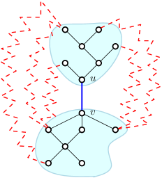
Figure 4. Insertion of edge $(u,v)$ affects the betweenness of nodes lying in the old shortest paths (red).

Algorithm 1 requires to add edges to the graph and to recompute the betweenness centrality $b_{v}$ of node $v$ after each edge insertion. Instead of recomputing it from scratch every time, we use a dynamic algorithm. The idea is to keep track of information regarding the graph and just update the parts that have changed as a consequence of the edge insertion. As described in Section 2, several algorithms for updating betweenness centrality after an edge insertion have been proposed. However, these algorithms update the betweenness of all nodes, whereas in Algorithm 1 we are interested in the betweenness of a single node. In this case, using an algorithm that recomputes the betweenness of all nodes would require a significant amount of superfluous operations. Let us consider the example shown in Figure 4.

The insertion of an edge $(u,v)$ does not only affect the betweenness of the nodes lying in the new shortest paths, but also that of the nodes lying in the old shortest paths between affected sources and affected targets (represented in red). Indeed, the fraction of shortest paths going through these nodes (and therefore their betweenness) has decreased as a consequence of the new insertion. Therefore, algorithms for updating the betweenness of all nodes have to walk over each old shortest path between node pairs whose distance has changed. However, we will show that if we are only interested in the betweenness of one particular node $x$, we can simply update the distances (and number of shortest paths) and check which of these updates affect the betweenness of $x$. Section 6.2 describes our new dynamic algorithm for updating the betweenness of a single node after an edge insertion. Notice that the algorithm could be used in any context where one needs to keep track of the betweenness of a single node after an edge insertion (or weight decrease) and not only for the betweenness improvement. Since our new algorithm builds on a recent dynamic betweenness algorithm called iBet (Bergamini et al., 2017), we first describe iBet in Section 6.1 and then explain how this can be modified to recompute the betweenness of a single node in Section 6.2.

6.1. iBet algorithm for updating the betweenness of all nodes

iBet (Bergamini et al., 2017) updates the betweenness of all nodes after an edge insertion or an edge weight decrease. Just as Brandes’s algorithm (Brandes, 2001), iBet is composed of two steps: a step where the pairwise distances and number of shortest paths are computed, and a step where the actual betweenness values are found.

Let us assume a new edge $(u,v)$ with weight $\omega^{\prime}_{u,v}$ is inserted into the graph, or that the weight of an existing edge $(u,v)\in E$ is decreased and set to a new value $\omega^{\prime}_{u,v}$. Then, let us name affected pairs the node pairs $(s,t)$ such that $d_{st}\geq d_{su}+\omega^{\prime}_{u,v}+d_{vt}$. Notice that these are the nodes for which either $(u,v)$ creates a shortcut (decreasing the distance), or creates one or more new shortest paths of the same length as the old distance. Also, let the affected sources of a node $t$ be the set $S(t)$ of nodes $\{s\in V:d_{st}\geq d_{su}+\omega^{\prime}_{u,v}+d_{vt}\}$ and let the set $T(s)$ of affected targets of $s$ be $T(s)=\{t\in v:d_{st}\geq d_{su}+\omega^{\prime}_{u,v}+d_{vt}\}$.

In (Bergamini et al., 2017) it was proven that if $(s,t)$ is an affected node pair, then $s\in S(v)$ and $t\in T(u)$. This allows us to reduce the search space of the affected pairs to the nodes whose distance to $v$ or from $u$ has changed (or their number of shortest paths). Thus, a first idea would be to identify the set $S(v)$ and the set $T(u)$, which can be done with two pruned BFSs, rooted in $u$ and $v$, respectively. For each node $s\in S(v)$ and each node $t\in T(u)$, we can compare the old distance $d_{st}$ with the one of a path going through edge $(u,v)$, namely $d_{su}+\omega^{\prime}_{u,v}+d_{vt}$, and update the distance and number of shortest paths accordingly. However, iBet is more efficient than this. Let a predecessor in a shortest path from $v$ to $t$ be any node $x$ such that $(x,t)\in E$ and $d_{vt}=d_{vx}+d_{xt}$, and let us denote this as $x\in P_{v}(t)$. Then, the following lemma holds.

Lemma 6.1.

(Bergamini et al., 2017) Let $\ t\in V$ be any node and $x\in P_{v}(t)$ be a predecessor of $t$ in the shortest paths from $v$. Then, $S(t)\subseteq S(x)$.

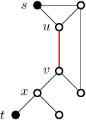
Figure 5. Insertion of edge $(u,v)$ creates a shortcut between $s$ and $t$, but also between $s$ and $x$.

Figure 5 explains this concept. The insertion of edge $(u,v)$ creates a shortcut between $s$ and $t$, making $(s,t)$ an affected pair. Similarly, the new edge creates a shortcut between $s$ and each predecessor of $t$ in the shortest path from $v$, i.e. $x$. Lemma 6.1 basically tells us that we do not need to check all pairs $(s,t)$ such that $s\in S(v)$ and $t\in T(u)$. On the contrary, for a given target $t$, we only need to check the nodes $s\in S(x)$, where $x$ is any node in $P_{v}(t)$. If we process the targets in increasing order of distance from $v$, this set will become smaller and smaller as we go down the BFS tree, saving unnecessary comparisons.

Clearly, what we described is only the update of the augmented APSP. After this, iBet also needs to update the betweenness scores of all the nodes that lie in some old or new shortest path between an affected pair. Since this part is not necessary when updating the betweenness of a single node, we will not describe this and refer the reader to (Bergamini et al., 2017) for more details.

Since the augmented APSP update of iBet was shown to be significantly faster than all existing algorithms, we use it as a building block for our incremental algorithm for the betweenness centrality of a single node, described in Section 6.2.

6.2. New dynamic algorithm for the betweenness of a single node

iBet stores the pairwise distances $d_{st}$ and the number of shortest paths $\sigma_{st}$ for each $s,t\in V$. When computing the betweenness of a specific node $x$, we also need the number $\sigma_{stx}$ of shortest paths between $s$ and $t$ that go through $x$. Then, we can compute betweenness by using its definition given in Eq. (1). In the following, we will assume that the graph $G$ is unweighted and connected, but the algorithm can be easily extended to weighted and disconnected graphs, in a way analogous to what has been done in (Bergamini et al., 2017). Our algorithm can be divided in two phases: an initialization phase, where pairwise distances, $\sigma_{(\cdot,\cdot)}$ and $\sigma_{(\cdot,\cdot)x}$ are computed and stored, and an update phase, where the data structures and the betweenness of node $x$ are updated as a consequence of the edge insertion.

6.2.1. Initialization

The initialization can be easily done by running a Single-Source Shortest Path (SSSP) from each node, as in the first phase of Brandes’s algorithm for betweenness centrality (Brandes, 2001). While computing distances from a source node $s$ to any other node $t$, we set the number $\sigma_{st}$ of shortest paths between $s$ and $t$ to the sum $\sum\sigma_{sp}$ over all predecessors $p$ in the shortest paths from $s$ (and we set $\sigma_{ss}=1$). This can be done for a node $s$ in $O(m)$ in unweighted graphs and in $O(m+n\log n)$ in weighted graphs (the cost of running a BFS or Dijkstra, respectively). Instead of discarding this information after each SSSP as in Brandes’s algorithm, we store both the distances $d_{(\cdot,\cdot)}$ and the numbers of shortest paths $\sigma_{(\cdot,\cdot)}$ in a matrix. After this, we can compute the number $\sigma_{(\cdot,\cdot)x}$ of shortest paths going through $x$. For each node pair $(s,t)$, $\sigma_{stx}$ is equal to $\sigma_{sx}\cdot\sigma_{xt}$ if $d_{st}=d_{sx}+d_{xt}$, and to 0 otherwise. The betweenness $b_{x}$ of $x$ can then be computed using the definition given in Eq. (1). This second part can be done in $O(n^{2})$ time by looping over all node pairs. Therefore the total running time of the initialization is $O(nm)$ for unweighted graphs and $O(n(m+n\log n))$ for weighted graphs, and the memory requirement is $O(n^{2})$, since we need to store three matrices of size $n\times n$ each.

6.2.2. Update

The update works in a way similar to iBet (see Section 6.1), with a few differences. Algorithm 2 gives an overview of the algorithm for betweenness update for a single node $x$, whereas Algorithm 3 and Algorithm 4 describe the update $\sigma_{(\cdot,\cdot)}$ and $\sigma_{(\cdot,\cdot)x}$ when $d_{st}>d_{su}+\omega^{\prime}_{uv}+d_{vt}$ and when $d_{st}=d_{su}+\omega^{\prime}_{uv}+d_{vt}$, respectively.

Algorithm 2 shares its structure with iBet. In Lines 2-2, after setting the new distance between $u$ and $v$, also $\sigma_{uv}$ and $\sigma_{uvx}$ are updated with either updateSigmaGR or updateSigmaEQ. Then, just like in iBet, the affected sources are identified with a pruned BFS rooted in $u$ on $G$ transposed (function findAffectedSources).

Then, a (pruned) BFS rooted in $v$ is started to find the affected targets for $u$ (Lines 2-2). In Lines 2-2, the neighbors $w$ of the affected target $t$ are visited and, if they are also affected (i.e. $d_{uw}\geq\omega^{\prime}_{uv}+d_{vw}$), they are enqueued. Also, $t$ is stored as the predecessor of $w$ (Line 2). In Lines 2-2, for each affected node pair $(s,t)$, we first subtract the old contribution $\sigma_{stx}/\sigma_{st}$ from the betweenness of $x$, then we recompute $d_{st}$, $\sigma_{st}$ and $\sigma_{stx}$ with either updateSigmaGR or updateSigmaEQ, and finally we add the new contribution $\sigma^{\prime}_{stx}/\sigma^{\prime}_{st}$ to $b_{x}$. Notice that, if $x$ did not lie in any shortest path between $s$ and $t$ before the edge insertion, $\sigma_{stx}=0$ and therefore $b_{x}$ is not decreased in Line 2. Analogously, if $x$ is not part of a shortest path between $s$ and $t$ after the insertion, $b_{x}$ is not increased in Line 2.

In the following, we analyze updateSigmaGR and updateSigmaEQ separately.

Algorithm: Incremental betweenness

Input : Graph $G=(V,E)$, edge update $(u,v,\omega^{\prime}_{uv})$, pairwise distances $d_{(\cdot,\cdot)}$, numbers $\sigma_{(\cdot,\cdot)}$ of shortest paths, numbers $\sigma_{(\cdot,\cdot)x}$ of shortest paths through $x$, betweenness value $b_{x}$ of $x$

Output : Updated $d_{(\cdot,\cdot)}$, $\sigma_{(\cdot,\cdot)}$, $\sigma_{(\cdot,\cdot)x}$ and $b_{x}$

Assume : boolean $vis(v)\text{ is false},\ \forall v\in V$

1 if $d_{uv}\geq\omega^{\prime}_{uv}$ then

2       if $d_{uv}>\omega^{\prime}_{uv}$ then

3             $d_{uv}\leftarrow\omega^{\prime}_{uv}$;

4             $\sigma_{uv},\sigma_{uvx}\leftarrow$updateSigmaGR($G,(u,v),d,\sigma,\sigma_{x}$);

5            

6      else

7             $\sigma_{uv},\sigma_{uvx}\leftarrow$updateSigmaEQ($G,(u,v),d,\sigma,\sigma_{x}$);

8            

9       $S(v)\leftarrow$ findAffectedSources($G,(u,v),d$);

10       $Q\leftarrow\emptyset$;

11       $P(v)\leftarrow v$;

12       $Q.push(v)$;

13       $vis(v)\leftarrow\text{true}$;

14       while $Q.length()>0$ do

15             $t=Q.front()$;

16             foreach $s\in\textnormal{{$S$}}(P(t))$ do

17                   if $d_{st}\geq d_{su}+\omega^{\prime}_{uv}+d_{vt}$ then

18                         if $x\neq s$ and $x\neq t$ then

19                               $b_{x}\leftarrow b_{x}-\sigma_{stx}/\sigma_{st}$;

20                              

21                        if $d_{st}>d_{su}+\omega^{\prime}_{uv}+d_{vt}$ then

22                               $\sigma_{st},\sigma_{stx}\leftarrow$updateSigmaGR($G,(u,v),d,\sigma,\sigma_{x}$);

23                               $d_{st}\leftarrow d_{su}+\omega^{\prime}_{uv}+d_{vt}$;

24                              

25                        else

26                               $\sigma_{st},\sigma_{stx}\leftarrow$updateSigmaEQ($G,(u,v),d,\sigma,\sigma_{x}$);

27                              

28                        if $x\neq s$ and $x\neq t$ then

29                               $b_{x}\leftarrow b_{x}+\sigma_{stx}/\sigma_{st}$;

30                              

31                        if $t\neq v$ then

32                               $S(t).insert(s)$;

33                              

34                        

35                  

36            foreach $w$ s.t. $(t,w)\in E$ do

37                   if not $vis(w)$ and $d_{uw}\geq\omega^{\prime}_{uv}+d_{vw}$ then

38                         $Q.push(w)$;

39                         $vis(w)\leftarrow\text{true}$;

40                         $P(w)\leftarrow t$;

41                        

42                  

43            

44      

ALGORITHM 2 Update of $b_{x}$ after an edge insertion

UpdateSigmaGR

Let us consider the case $d_{st}>d_{su}+\omega^{\prime}_{uv}+d_{vt}$. In this case, all the old shortest paths are discarded, as they are not shortest paths any longer, and all the new shortest paths go through edge $(u,v)$. Therefore, we can set the new number $\sigma^{\prime}_{st}$ of shortest paths between $s$ and $t$ to $\sigma_{su}\cdot\sigma_{vt}$. Since all old shortest paths should be discarded, also $\sigma_{stx}$ depends only on the new shortest paths and not on whether $x$ used to lie in some shortest paths between $s$ and $t$ before the edge insertion. Depending on the position of $x$ with respect to the new shortest paths, we can define three cases, depicted in Figure 6. In Case (a) (left), $x$ lies in one of the shortest paths between $s$ and $u$. This means that it also lies in some shortest paths between $s$ and $t$. In particular, the number of these paths $\sigma^{\prime}_{stx}$ is equal to $\sigma_{sux}\cdot\sigma_{vt}$. Notice that no shortest paths between $s$ and $u$ can be affected (see (Bergamini et al., 2017)) and therefore $\sigma_{sux}=\sigma^{\prime}_{x}(s,u)$. In Case (b) (center), $x$ lies in one of the shortest paths between $v$ and $t$. Analogously to Case 1, the new number of shortest paths between $s$ and $t$ going through $x$ is $\sigma^{\prime}_{stx}=\sigma_{su}\cdot\sigma_{vtx}$. Notice that Case (a) and Case (b) cannot both be true at the same time. In fact, if $d_{su}=d_{sx}+d_{xu}$ and $d_{vt}=d_{vx}+d_{xt}$, we would have that $d^{\prime}_{st}=d_{su}+\omega^{\prime}_{uv}+d_{vt}=d_{sx}+d_{xu}+\omega^{\prime}_{uv}+d_{vx}+d_{xt}>d_{sx}+d_{xt}$, which is impossible, since $d^{\prime}_{st}$ is the shortest-path distance between $s$ and $t$. Therefore, at least one among $\sigma_{sux}$ and $\sigma_{vtx}$ must be equal to 0. Finally, in Case (c) (right), $\sigma_{sux}$ and $\sigma_{vtx}$ are both equal to 0, meaning that $x$ does not lie on any new shortest path between $s$ and $t$. Once again, this is independent on whether $x$ lied in an old shortest path between $s$ and $t$ or not. Algorithm 3 shows the computation of $\sigma^{\prime}_{st}$ and $\sigma^{\prime}_{stx}$. Notice that, in the computation of $\sigma^{\prime}_{stx}$, the first addend is greater than zero only in Case (a) and the second only in Case (b).

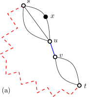
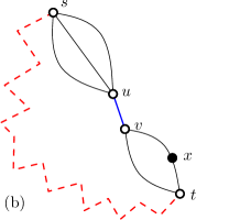
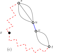
Figure 6. Possible positions of $x$ with respect to the new shortest paths after the insertion of edge $(u,v)$. On the left, $x$ lies between the source $s$ and $u$. In the center, $x$ lies between $v$ and the target $t$. On the right, $x$ does not lie on any new shortest path between $s$ and $t$.

Algorithm: UpdateSigmaGR

Input : Graph $G=(V,E)$, edge insertion $(u,v)$, pairwise distances $d_{(\cdot,\cdot)}$, numbers $\sigma_{(\cdot,\cdot)}$ of shortest paths, numbers $\sigma_{(\cdot,\cdot)x}$ of shortest paths through $x$

Output : Updated $\sigma^{\prime}_{st}$, $\sigma^{\prime}_{stx}$

1 $\sigma^{\prime}_{st}\leftarrow\sigma_{su}\cdot\sigma_{vt}$;

2 $\sigma^{\prime}_{stx}\leftarrow\sigma_{sux}\cdot\sigma_{vt}+\sigma_{su}\cdot\sigma_{vtx}$;

3 return $\sigma^{\prime}_{st}$, $\sigma^{\prime}_{stx}$;

ALGORITHM 3 Update of $\sigma_{st}$ and $\sigma_{stx}$ when $(u,v)$ creates new shortest paths of length smaller than $d_{st}$

UpdateSigmaEQ

Let us now consider the case $d_{st}=d_{su}+\omega^{\prime}_{uv}+d_{vt}$. Here all the old shortest paths between $s$ and $t$ are still valid and, in addition to them, new shortest paths going through $(u,v)$ have been created. Therefore, the new number of shortest paths $\sigma^{\prime}_{st}$ is simply $\sigma_{st}+\sigma_{su}\cdot\sigma_{vt}$. Notice that we never count the same path multiple times, since all new paths go through $(u,v)$ and none of the old paths does. Also all old shortest paths between $s$ and $t$ through $x$ are still valid, therefore $\sigma^{\prime}_{stx}$ is given by the old $\sigma_{stx}$ plus the number of new shortest paths going through both $x$ and $(u,v)$. This number can be computed as described for updateSigmaGR according to the cases of Figure 6. Algorithm 4 shows the computation of $\sigma^{\prime}_{st}$ and $\sigma^{\prime}_{stx}$.

Algorithm: UpdateSigmaEQ

Input : Graph $G=(V,E)$, edge insertion $(u,v)$, pairwise distances $d_{(\cdot,\cdot)}$, numbers $\sigma_{(\cdot,\cdot)}$ of shortest paths, numbers $\sigma_{(\cdot,\cdot)x}$ of shortest paths through $x$

Output : Updated $\sigma^{\prime}_{st}$, $\sigma^{\prime}_{stx}$

1 $\sigma^{\prime}_{st}\leftarrow\sigma_{st}+\sigma_{su}\cdot\sigma_{vt}$;

2 $\sigma^{\prime}_{stx}\leftarrow\sigma_{stx}+\sigma_{sux}\cdot\sigma_{vt}+\sigma_{su}\cdot\sigma_{vtx}$;

3 return $\sigma^{\prime}_{st}$, $\sigma^{\prime}_{stx}$;

ALGORITHM 4 Update of $\sigma_{st}$ and $\sigma_{stx}$ when $(u,v)$ creates new shortest paths of length equal to $d_{st}$

6.3. Time complexities

6.3.1. Dynamic betweenness algorithm

Let us define the extended size $||A||$ of a set of nodes $A$ as the sum of the number of nodes in $A$ and the number of edges that have a node of $A$ as their endpoint. Then, the following proposition holds.

Proposition 6.2.

The running time of Algorithm 2 for updating the betweenness of a single node after an edge insertion $(u,v)$ is $\Theta(||S(v)||+||T(u)||+\sum_{y\in T(u)}|S(P(y))|)$.

Proof.

The function findAffectedSources in Line 2 identifies the set of affected sources starting a BFS in $v$ and visiting only the nodes $s$ such that $d_{su}+\omega^{\prime}_{uv}+d_{vt}\leq d_{st}$. This takes $\Theta(||S(v)||)$, since this partial BFS visits all nodes in $S(v)$ and their incident edges. Then, the while loop of Lines 2 - 2 (excluding the part in Lines 2 - 2) identifies all the affected targets $T(u)$ with a partial BFS. This part requires $\Theta(||T(u)||)$ operations, since all affected targets and their incident edges are visited. In Lines 2 - 2, for each affected node $t\in T(u)$, all the affected sources of the predecessor $P(t)$ of $t$ are scanned. This part requires in total $\Theta(\sum_{t\in T(u)}|S(P(t))|)$ operations, since for each node in $S(P(t))$, Lines 2 - 2 require constant time. ∎

Notice that, since $S(P(y))$ is $O(n)$ and both $||T(u)||$ and $||S(v)||$ are $O(n+m)$, the worst-case complexity of Algorithm 2 is $O(n^{2})$ (assuming $m=\Omega(n)$). This matches the worst-case running time of the augmented APSP update of iBet. However, notice that iBet needs a second step to update the betweenness of all nodes, which is more expensive and requires $\Theta(nm)$ operations in the worst case. Also, this introduces a contrast between the static and the incremental case: Whereas the static computation of one node’s betweenness has the same complexity as computing it for all nodes (at least no algorithm for computing it for one node faster than computing it for all nodes exists so far), in the incremental case the betweenness update of a single node can be done in $O(n^{2})$, whereas there is no algorithm faster than $O(nm)$ for the update of all nodes.

6.3.2. Greedy algorithm for betweenness maximization

We can improve the running time of Algorithm Greedy by using the dynamic algorithm for betweenness centrality instead of the recomputation from scratch. In fact, at Line 1 of Algorithm Greedy, we add an edge $\{u,v\}$ to the graph and compute the betweenness in the new graph, for each node $u$ in $V\setminus N_{v}(S)$. If we compute the betweenness by using the from-scratch algorithm, this step requires $O(nm)$ and this leads to an overall complexity of $O(kn^{2}m)$. At Line 1 , instead of recomputing betweenness on the new graph from scratch, we can use Algorithm 2. As we proved previously, its worst-case complexity is $O(n^{2})$. This leads to an overall worst-case complexity of $O(kn^{3})$ for Greedy. However, in Section 7.2 we will show that Greedy is actually much faster in practice.

7. Experimental evaluation

In our experiments, we evaluate the performance of Greedy both in terms of quality of the solution found (Section 7.1) and in terms of its running time (Section 7.2). All algorithms compared in our experiments are implemented in C++, building on the open-source NetworKit (Staudt et al., 2016) framework. The experiments were done on a machine equipped with 256 GB RAM and a 2.7 GHz Intel Xeon CPU E5-2680 having 2 sockets with 8 cores each. To make the comparison with previous work more meaningful, we use only one of the 16 cores. The machine runs 64 bit SUSE Linux and we compiled our code with g++-4.8.1 and OpenMP 3.1.

For our experiments, we consider a set of real-world networks belonging to different domains, taken from SNAP (Leskovec and Krevl, 2014), KONECT (Kunegis, 2013), Pajek (Batagelj and Mrvar, 2006), and the 10th DIMACS Implementation Challenge (Bader et al., 2014). The properties of the networks are reported in Table 2 (directed graphs) and in Table 3 (undirected graphs).

7.1. Solution quality

In this section we evaluate Greedy in terms of accuracy and we compare it both with the optimum and with some alternative baselines.

To speed up the computation of Greedy (and therefore to target larger graphs), we do not recompute betweenness from scratch in Line 1 of Algorithm 1, but we use the dynamic algorithm described in Section 6. Notice that this does not affect the solution found by the algorithm, only its running time, which is reported in Section 7.2. Since computing the optimum by examining all possible $k$-tuples would be too expensive even on small graphs, we use an Integer Programming (IP) formulation, described in the following paragraph.

7.1.1. IP formulation for MBI on directed graphs

Let $S$ be a solution to an instance of MBI. Given a node $v$, we define a variable $x_{u}$ for each node $u\in V\setminus(N_{v}\cup\{v\})$

$$x_{u}=\begin{cases}1&\mbox{if }(u,v)\in S\\ 0&\mbox{otherwise.}\end{cases}$$

We define a variable $y_{st}$ for each $s,t\in V\setminus\{v\}$, $s\neq t$.

$$y_{st}=\begin{cases}1&\mbox{If all shortest paths from }s\mbox{ to }t\mbox{ in }G(S)\mbox{ pass through node }v\\ 0&\mbox{otherwise.}\end{cases}$$

For each pair of nodes $s,t\in V\setminus\{v\}$, $s\neq t$, we denote by $A(s,t)$ the set of nodes $u$ not in $N_{v}$ such that all the shortest paths between $s$ and $t$ in $G(\{(u,v)\})$ pass through edge $(u,v)$ and hence through node $v$. Note that in this case, $d_{st}>d_{st}(\{(u,v)\})$ and hence $A(s,t)$ is defined as $A(s,t)=\{u~{}|~{}d_{st}>d_{st}(\{(u,v)\})\}$. Set $B(s,t)$ is defined as the set of nodes $u$ not in $N_{v}$ such that at least a shortest path between $s$ and $t$ in $G(\{(u,v)\})$ does not pass through edge $(u,v)$ and hence $B(s,t)=V\setminus(A(s,t)\cup N_{v})$. We denote by $\bar{\sigma}_{stv}(u)$ the number of shortest paths from $s$ to $t$ in $G(\{(u,v)\})$ passing through edge $(u,v)$.

The following non linear formulation solves the MBI problem:

(5) $$\max \sum_{\begin{subarray}{c}s,t\in V\\ s\neq t;s,t\neq v\end{subarray}}\left((1-y_{st})\frac{\sigma_{stv}+\sum_{u\in B(s,t)}x_{u}\bar{\sigma}_{stv}(u)}{\sigma_{st}+\sum_{u\in B(s,t)}x_{u}\bar{\sigma}_{stv}(u)}+y_{st}\right)$$

(6) subject to $$\sum_{u\in A(s,t)}x_{u}\geq y_{st}, s,t\in V\setminus\{v\},s\neq t$$

$$\sum_{u\in V\setminus(N_{v}\cup\{v\})}x_{u}\leq k,$$

$$x_{u},y_{st}\in\{0,1\} s\in V\setminus\{v\},t\in V\setminus\{v,s\}$$

Let us consider a solution $S$ to the above formulation. In the case that $y_{st}=1$, for some pair of nodes $s,t\in V\setminus\{v\}$, $s\neq t$, then Constraint (6) implies that, for at least a node $u\in A(s,t)$, variable $x_{u}$ must be set to 1 and hence all the shortest paths between $s$ and $t$ in $G(S)$ pass through $v$. In this case, the term corresponding to pair $(s,t)$ in the objective function (5) is correctly set to be equal to 1.

If $y_{st}=0$ and $x_{u}=0$, for each $u\in A(s,t)$, then the number of shortest paths between $s$ and $t$ in $G(S)$ passing through $v$ is equal to $\sigma_{stv}+\sum_{u\in B(s,t)}x_{u}\bar{\sigma}_{stv}(u)$ and the overall number of shortest paths between $s$ and $t$ in $G(S)$ is equal to $\sigma_{st}+\sum_{u\in B(s,t)}x_{u}\bar{\sigma}_{stv}(u)$. In this case, the term corresponding to pair $(s,t)$ in the objective function (5) is correctly set to be equal to $\frac{\sigma_{stv}+\sum_{u\in B(s,t)}x_{u}\bar{\sigma}_{stv}(u)}{\sigma_{st}+\sum_{u\in B(s,t)}x_{u}\bar{\sigma}_{stv}(u)}$.

Note that, $\frac{\sigma_{stv}+\sum_{u\in B(s,t)}x_{u}\bar{\sigma}_{stv}(u)}{\sigma_{st}+\sum_{u\in B(s,t)}x_{u}\bar{\sigma}_{stv}(u)}\leq 1$ and therefore a solution in which $y_{st}=0$ and $x_{u}=1$, for some $u\in A(s,t)$ is at least as good as a solution in which $y_{st}$ is set to 1 instead of 0 and the other variables are unchanged. Hence, we can assume without loss of generality that the case in which $y_{st}=0$ and $x_{u}=1$, for some $u\in A(s,t)$, cannot occur in an optimal solution.

We solve the program with the Mixed-Integer Nonlinear Programming Solver Couenne (Belotti et al., 2009) and measure the approximation ratio of the greedy algorithm on three types of randomly generated directed networks, namely directed Preferential Attachment (in short, PA) (Bollobás et al., 2003), Copying (in short, COPY) (Kumar et al., 2000), Compressible Web (in short, COMP) (Chierichetti et al., 2009). For each graph type, we generate 5 different instances with the same size. We focus our attention on twenty vertices $v$, which have been chosen on the basis of their original betweenness ranking. In particular, we divide the list of vertices, sorted by their original ranking, in four intervals, and choose five random vertices uniformly at random in each interval. In each experiment, we add $k=\{1,2,...,7\}$ edges. We evaluate the quality of the solution produced by the greedy algorithm by measuring its approximation ratio and we report the results in Table 1.

Table 1. Comparison between the Greedy algorithm and the optimum. The first three columns report the type and size of the graphs; the fourth column reports the approximation ratio.

Graph	Nodes	Edges	Min. approx. ratio
PA	100	130	1
COPY	100	200	0.98
COMP	100	200	0.98
COMP	100	500	0.96

The experiments clearly show that the experimental approximation ratio is by far better than the theoretical one proven in the previous section. In fact, in all our tests, the experimental ratio is always greater than 0.96.

7.1.2. Results for real-world directed networks

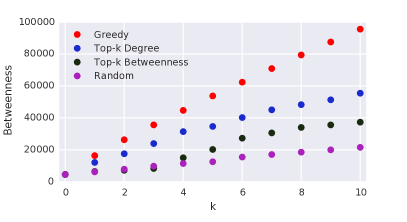
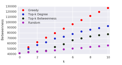
Figure 7. Betweenness of the pivot as a function of the number $k$ of inserted edges for the four heuristics. The plots refer to two different pivots in the munmun-digg-reply graph.

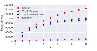
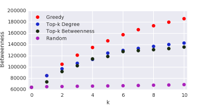
Figure 8. Betweenness of the pivot as a function of the number $k$ of inserted edges for the four heuristics. The plots refer to two different pivots in the linux graph.

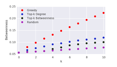
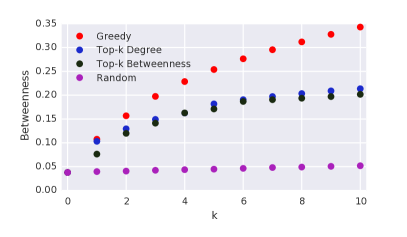
Figure 9. Percentage betweenness of the pivot as a function of the number $k$ of inserted edges for the four heuristics. Left: average results for the munmun-digg-reply graph. Right: average results for the linux graph.

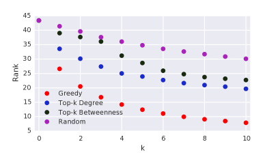
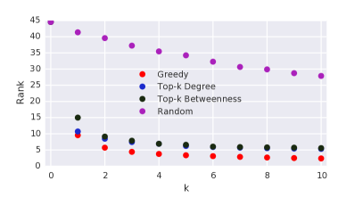
Figure 10. Percentage rank of the pivot as a function of the number $k$ of inserted edges for the four heuristics. Left: average results for the munmun-digg-reply graph. Right: average results for the linux graph.

We also analyze the performance of Greedy on the real-world directed networks of Table 2 (Section 7.2). Since finding the optimum on these networks would take too long, we compare the solution of Greedy with the following three baselines:

• Top-k Degree: the algorithm that connects the $k$ nodes having the highest degree to $v$;

• Top-k Betweenness: the algorithm that connects the $k$ nodes having the highest betweenness centrality to $v$;

• Random: the algorithm that connects $k$ nodes extracted uniformly at random to $v$.

For each graph, we pick one node at random, compute its betweenness on the initial graph and try to increase it with the four heuristics. We refer to the selected node as pivot. Since the results may vary depending on the initial betweenness of the pivot, we also repeat each experiment with 10 different pivots. In each experiment, we add $k=\{1,2,...,10\}$ edges and compute the ranking and betweenness of the pivot after each insertion.

Figure 7 shows the results for the munmun-digg-reply graph, using two different pivots. In particular, the plot on the left shows the betweenness improvement for a node with an initially low betweenness score (close to 0), whereas the one on the right refers to a node that starts with a higher betweenness value (about 40000). Although the final betweenness scores reached by the two nodes differ, we see that the relative performance of the four algorithms is quite similar among the two pivots. A similar behavior can be observed for all other tested pivots. Figure 8 reports the results for two different pivots chosen from the linux graph. Again, we notice that the relative performance of the four algorithms is basically the same. Since the same is true also for the other tested graphs, in the following we simply report the average values among the samples.

Figure 9 reports the average results (over the sampled pivots) for munmun-digg-reply (left) and linux (right). We define the percentage betweenness of a node $v$ as $b_{v}\cdot\frac{100}{(n-1)(n-2)}$, where $b_{v}$ is the betweenness of $v$ and $(n-1)(n-2)$ represents the maximum theoretical betweenness a node can have in a graph with $n$ nodes. For each value of $k$, the plots show the average percentage betweenness of a pivot after the insertion of $k$ edges (each point represents the average over the 10 pivots). Clearly, the pivot’s betweenness after $k$ insertions is a non-decreasing function of $k$, since the insertion of an edge can only increase (or leave unchanged) the betweenness of one of its endpoints. In both plots, Greedy outperforms the other heuristics. For example, after 10 edge insertions, the average betweenness of a pivot in the munmun-digg-reply graph is 81460 with Greedy, 43638 with Top-k Degree, 36690 with Top-k Betweenness and 28513 with Random. A similar behavior can be observed for the average ranks of the pivots, reported in Figure 10. The figures report the percentage ranks, i.e. the ranks multiplied by $\frac{100}{n}$, since $n$ is the maximum rank a node can have in a graph with $n$ nodes. This can be seen as the fraction of nodes with higher betweenness than the pivot. On munmun-digg-reply , the average initial rank is 2620 (about 43%). After 10 insertions, the rank obtained using Greedy is 476 (about 7%), whereas the one obtained by the other approaches is never lower than 1188 (about 19%). It is interesting to notice that 3 edge insertions with Greedy yield a rank of 1011, which is better than the one obtained by the other approaches after 10 insertions. Similarly, also on the linux graph, 3 iterations of Greedy are enough to bring down the rank from 2498 (45.6%) to 247 (4.4%), whereas the other approaches cannot go below 299 (5.3%) with 10 iterations.

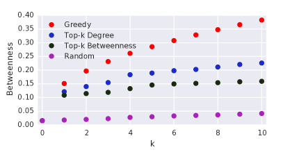
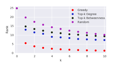
Figure 11. Average results over all directed networks. On the left, average percentage betweenness of the pivots as a function of $k$. On the right, average percentage rank of the pivots.

Similar results can be observed on the other tested (directed) instances. Figure 11 reports the average results over all directed networks, both in terms of betweenness (left) and rank (right) improvement. The initial average betweenness of the sample pivots is 0.015%. Greedy is by far the best approach, with an average final percentage betweenness (after 10 iterations) of 0.38% and an average final percentage rank of 1.4%. As a comparison, the best alternative approach (Top-k Degree) yields a percentage betweenness of 0.22% and a percentage rank of 7.3%. Not surprisingly, the worst approach is Random, which in 10 iterations yields a final percentage betweenness of 0.04% and an average percentage rank of 10.2%. On average, a single iteration of Greedy is sufficient for a percentage rank of 5.5%, better than the one obtained by all other approaches in 10 iterations. Also, it is interesting to notice that in our experiments Top-k Degree performs significantly better than Top-k Betweenness. This means that, for the betweenness of a node in a directed graph, it is more important to have incoming edges from nodes with high out-degree than with high betweenness. We will see in the following that our results show a different behavior for undirected graphs.

Also, notice that, although the percentage betweenness scores are quite low, the improvement using Greedy is still large: with 10 insertions, on average the scores change from an initial 0.015% to 0.38%, which is about 25 times the initial value.

7.1.3. Results for real-world undirected graphs

Although it was proven that Greedy has an unbounded approximation ratio for undirected graphs (D’Angelo et al., 2016), it is still not clear how it actually performs in practice. In (D’Angelo et al., 2016), the authors performed some preliminary experiments in which they showed that the greedy algorithm provides a solution slightly better than the Top-k Betweenness algorithm. However, they analyzed only very small networks (with few hundreds of nodes), due to the high complexity of a straightforward implementation of the Greedy algorithm. In what follows, we compare Greedy with other baselines on graphs with up to $10^{4}$ nodes and $10^{5}$ edges. This is made possible by combining Greedy with the dynamic algorithm described in Section 6 (note that using the dynamic algorithm only influences the running times of Greedy, but not its results). In particular, we compare Greedy with Top-k Betweenness, Top-k Degree and Random also on several undirected real-world networks, listed in Table 3 of Section 7.2.

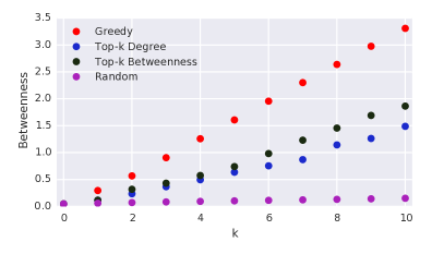
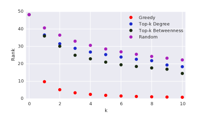
Figure 12. Average results over all undirected networks. On the left, average percentage betweenness of the pivots as a function of $k$. On the right, average percentage rank of the pivots.

Figure 12 shows the percentage betweenness and ranking, averaged over the undirected networks of Table 3. Also in this case, Greedy outperforms the other heuristics. In particular, the average initial betweenness of the pivots in the different graphs is 0.05%. After 10 iterations, the betweenness goes up to 3.7% with Greedy, 1.6% with Top-k Degree, 2.1% with Top-k Betweenness and only 0.17% with Random. The average initial rank is 45%. Greedy brings it down to 0.7% with ten iterations and below 5% already with two. Using the other approaches, the average rank is always worse than 10% for Top-k Betweenness, 15% for Top-k Degree and 20% for Random. As mentioned before, differently from directed graphs, Top-k Betweenness performs significantly better than Top-k Degree in undirected graphs.

Also, notice that in undirected graphs the percentage betweenness scores of the nodes in the examined graphs are significantly larger than those in the directed graphs. This could be due to the fact that many node pairs have an infinite distance in the examined directed graphs, meaning that these pairs do not contribute to the betweenness of any node. Also, say we want to increase the betweenness of $x$ by adding edge $(v,x)$. The pairs $(s,t)$ for which we can have a shortcut (leading to an increase in the betweenness of $x$) are limited to the ones such that $s$ can reach $v$ and such that $t$ is reachable from $x$, which might be a small fraction of the total number of pairs. On the contrary, most undirected graphs have a giant connected component containing the greatest majority of the nodes. Therefore, it is very likely that a pivot belongs to the giant component or that it will after the first edge insertion.

It is interesting to notice that, despite the unbounded approximation ratio, the improvement achieved by Greedy on undirected graphs is even larger than for the directed ones: on average 74 times the initial score.

7.2. Running time evaluation

In this section we evaluate the running time of the dynamic algorithm for betweenness centrality computation. We used the same experimental setting used in Section 7.1. Since some of the algorithms we use for comparison work only on unweighted graphs, all the tested networks are unweighted (although we recall that our algorithm described in Section 6.2 can handle also weighted graphs).

7.2.1. Evaluation of the dynamic algorithm for the betweenness of one node

In the following, we refer to our incremental algorithm for the update of the betweenness of a single node as SI (Single-node Incremental). Since there are no other algorithms specifically designed to compute or update the betweenness of a single node, we also use the static algorithm by Brandes (Brandes, 2001) and the dynamic algorithm by Bergamini et al. (Bergamini et al., 2017) for a comparison (the one by Brandes was already in NetworKit). Indeed, the algorithm by Brandes (which we refer to as Stat, from Static) is the best known algorithm for static computation of betweenness and the one by Bergamini et al. (which we name AI, from All-nodes Incremental) has been shown to outperform other dynamic algorithms (Bergamini et al., 2017).

To compare the running times of the algorithms for betweenness centrality, we choose a node $x$ at random and we assume we want to compute the betweenness of $x$. Then, we add an edge to the graph, also chosen uniformly at random among the node pairs $(u,v)$ such that $(u,v)\notin E$. After the insertion, we use the three algorithms to update the betweenness centrality of $x$ and compare their running times. We recall that Stat is a static algorithm, which means that we can only run it from scratch on the graph after the edge insertion. On each graph, we repeat this 100 times and report the average running time obtained by each of the algorithms.

Table 2. Average running times of the betweenness algorithms on directed real-world graphs. The last two columns report the standard deviation of the running times of AI and SI over the 100 edge insertions.

Graph	Nodes	Edges	Time Stat [s]	Time AI [s]	Time SI [s]	STD AI [s]	STD SI [s]
subelj-jung	6 120	50 535	1.25	0.0019	0.0002	0.0036	0.0005
wiki-Vote	7 115	100 762	8.18	0.0529	0.0015	0.0635	0.0038
elec	7 118	103 617	8.67	0.0615	0.0019	0.0858	0.0053
freeassoc	10 617	63 788	14.96	0.1118	0.0034	0.1532	0.0036
dblp-cite	12 591	49 728	5.04	0.1726	0.0071	0.7905	0.0451
subelj-cora	23 166	91 500	34.08	0.3026	0.0327	1.1598	0.1575
ego-twitter	23 370	33 101	8.47	0.0062	0.0001	0.0576	0.0003
ego-gplus	23 628	39 242	10.01	0.0024	0.0001	0.0026	0.0000
munmun-digg	30 398	85 247	78.09	0.2703	0.0073	0.2539	0.0099
linux	30 837	213 424	34.75	0.0692	0.0108	0.3019	0.0637

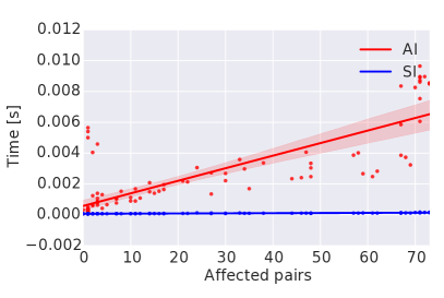
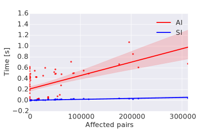
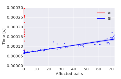
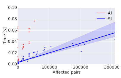
Figure 13. Top: Running time of AI and SI as a function of the number of affected node pairs for two directed graphs (left: ego-gplus, right: munmun-digg). Bottom: Same as the two plots above, but zoomed on the running times of SI. The points are the computed running times, the lines are the results of a linear regression and the area around the lines is a 95% confidence interval for the regression.

Table 3. Average running times of the betweenness algorithms on undirected real-world graphs. The last two columns report the standard deviation of the running times of AI and SI over the 100 edge insertions.

Graph	Nodes	Edges	Time Stat [s]	Time AI [s]	Time SI [s]	SD AI [s]	SD SI [s]
Mus-musculus	4 610	5 747	2.87	0.0337	0.0037	0.0261	0.0024
HC-BIOGRID	4 039	10 321	5.32	0.1400	0.0083	0.1450	0.0119
Caenor-eleg	4 723	9 842	4.75	0.0506	0.0025	0.0406	0.0014
ca-GrQc	5 241	14 484	4.15	0.0377	0.0033	0.0245	0.0017
advogato	7 418	42 892	12.65	0.1820	0.0024	0.1549	0.0008
hprd-pp	9 465	37 039	29.19	0.2674	0.0053	0.1873	0.0021
ca-HepTh	9 877	25 973	21.57	0.1404	0.0095	0.1108	0.0053
dr-melanog	10 625	40 781	38.18	0.2687	0.0067	0.2212	0.0029
oregon1	11 174	23 409	23.77	0.5676	0.0037	0.5197	0.0020
oregon2	11 461	32 730	27.98	0.5655	0.0039	0.5551	0.0026
Homo-sapiens	13 690	61 130	68.06	0.5920	0.0079	0.4203	0.0035
GoogleNw	15 763	148 585	76.17	2.4744	0.0044	4.1075	0.0045
CA-CondMat	21 363	91 342	168.44	1.1375	0.0486	0.7485	0.0358

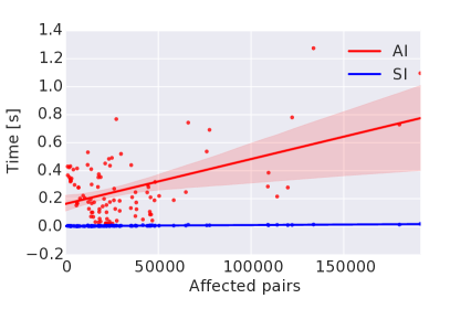
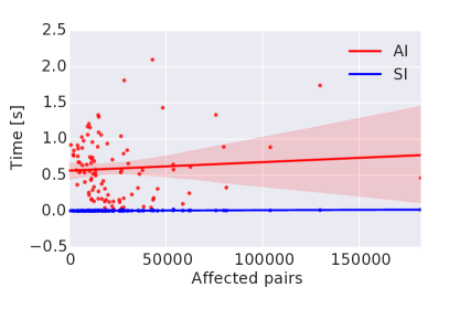
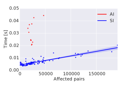
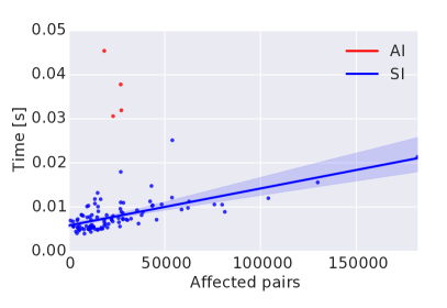
Figure 14. Top: Running time of AI and SI as a function of the number of affected node pairs for two undirected graphs (left: dr-melanog, right: Homo-sapiens). Bottom: same as the two plots above, but zoomed on the running times of SI. The points are the computed running times, the lines are the results of a linear regression and the area around the lines is a 95% confidence interval for the regression.

Table 2 and Table 3 show the running times for directed and undirected graphs, respectively. As expected, both dynamic algorithms AI and SI are faster than the static approach and SI is the fastest among all algorithms. This is expected, since SI is the one that performs the smallest number of operations. Also, notice that the standard deviation of the running times of both AI and SI is very high, sometimes even higher than the average. This is actually not surprising, since different edge insertion might affect portions of the graph of very different sizes. Figure 13 and Figure 14 report the running times of AI and SI as a function of the number of affected node pairs for two directed and undirected graphs, respectively (similar results can be observed for the other tested graphs). As expected, the running time of both algorithms (as well as the difference between the running time of AI and that of SI) mostly increases as the number of affected pairs increases. However, AI presents a much larger deviation than SI. This is due to the fact that its running time also depends on the number of nodes that used to lie in old shortest paths between the affected pairs. Indeed, the number of nodes whose betweenness gets affected does not only depend on the number of affected pairs (which we recall to be the ones for which the edge insertion creates a shortcut or a new shortest paths), but also on how many shortest paths there used to be between the affected pairs before the insertion and how long these paths were.

Table 4. Speedups on the static algorithm and on the dynamic algorithm for all nodes on directed networks. For both Stat and AI, the first column reports the geometric mean of the speedups over the 100 insertions, the second column reports the maximum speedups and the third column the minimum speedup.

	Speedups on Stat			Speedups on AI
Graph	Geometric mean	Maximum	Minimum	Geometric mean	Maximum	Minimum
subelj-jung	24668.3	67477.6	342.9	10.0	63.7	1.1
wiki-Vote	23779.8	381357.7	275.6	39.3	310.7	1.0
elec	21560.5	408629.3	175.6	32.1	285.1	1.1
freeassoc	6783.2	330333.4	707.5	13.0	94.0	1.1
dblp-cite	24745.7	140950.0	11.4	13.3	314.5	1.1
subelj-cora	18936.5	543630.2	22.9	32.4	257.5	1.0
ego-twitter	111597.2	134716.0	3169.2	4.0	216.3	1.0
ego-gplus	115936.2	154869.5	57650.6	14.6	74.5	1.1
munmun-digg	34299.5	998564.0	1796.8	30.7	188.3	1.2
linux	103469.6	433745.5	59.5	32.1	94.6	1.5

Table 5. Speedups on the static algorithm and on the dynamic algorithm for all nodes on undirected networks. For both Stat and AI, the first column reports the geometric mean of the speedups over the 100 insertions, the second column reports the maximum speedups and the third column the minimum speedup.

	Speedups on Stat			Speedups on AI
Graph	Geometric mean	Maximum	Minimum	Geometric mean	Maximum	Minimum
Mus-musculus	1031.2	174166.8	191.4	7.7	21.9	1.7
HC-BIOGRID	962.3	4060.6	56.7	17.0	51.1	4.5
Caenor-eleg	2152.2	293172.8	474.6	15.0	49.4	1.3
ca-GrQc	1517.5	220289.2	351.8	10.0	22.8	2.1
advogato	5819.0	698406.6	2860.5	43.4	192.7	1.9
hprd-pp	5846.6	10852.3	1696.6	39.2	119.5	3.2
ca-HepTh	2642.6	432794.2	549.2	12.3	35.7	2.8
dr-melanog	6105.9	10589.7	1869.7	29.9	88.3	3.1
oregon1	7407.4	733008.3	1562.3	72.6	493.4	2.4
oregon2	9192.5	617710.0	1595.8	68.8	470.5	2.5
Homo-sapiens	9216.4	17177.4	2706.2	57.0	165.2	3.4
GoogleNw	34967.2	505509.9	3799.3	137.3	1560.3	2.9
CA-CondMat	4073.9	10690.6	537.8	20.8	69.4	2.8

Table 4 and Table 5 show the speedups of SI on AI and those of SI on Stat, for directed and undirected graphs, respectively. Although the speedups vary considerably among the networks and the edge insertions, SI is always at least as fast as AI and up to 1560 times faster (maximum speedup for GoogleNw). On average (geometric mean of the average speedups over the tested networks), SI is 29 times faster than AI for undirected graphs and 18 times faster for directed graphs. The high speedups on the dynamic algorithm for all nodes is due to the fact that, when focusing on a single node, we do not need to update the scores of all the nodes that lie in some shortest path affected by the edge insertion. On the contrary, for each affected source node $s$, AI has to recompute the change in dependencies by iterating over all nodes that lie in either a new or an old shortest path from $s$. As a result, SI is extremely fast: on all tested instances, its running time is always smaller than 0.05 seconds, whereas AI can take up to seconds to update betweenness.

Compared to recomputation, SI is on average about 4200 times faster than Stat on directed and about 33000 times on undirected graphs (geometric means of the speedups). Since SI has shown to outperform other approaches in the context of updating the betweenness centrality of a single node after an edge insertion, we use it to update the betweenness in the greedy algorithm for the Maximum Betweenness Improvement problem (Section 5). Therefore, in all the following experiments, what we refer to as Greedy is the Algorithm of Section 5 where we recompute betweenness after each edge insertion with SI.

7.2.2. Running times of the greedy algorithm for betweenness maximization

In Section 5, we already showed that Greedy outperforms all other heuristics in terms of solution quality, both on directed and on undirected graphs (although we recall that the theoretical guarantee on the approximation ratio holds only for directed graphs). In this section, we report the running times of Greedy, using SI to recompute betweenness. Table 6 and Table 7 show the results on directed and undirected graphs, respectively. For each value of $k$, the tables show the running time required by Greedy when $k$ edges are added to the graph. Notice that this is not the running time of the $k$th iteration, but the total running time of Greedy for a certain value of $k$. Since on directed graphs the betweenness of $x$ is a submodular function of the solutions for MBI (see Theorem 5.2), we can speed up the computation for $k>1$ (see Algorithm 5). This technique was originally proposed in (Minoux, 1978) and it was used in (Crescenzi et al., 2016) to speed up the greedy algorithm for harmonic centrality maximization. Let $\Delta b_{v}(u)=b_{v}(S\cup\{(u,v)\})-b_{v}(S)$, where $S$ is the solution computed at some iteration $i^{\prime}<i$, that is, $\Delta b_{v}(u)$ is the increment to $b_{v}$ given by adding the edge $(u,v)$ to $S$ at iteration $i^{\prime}$. Let $LB$ be the current best solution at iteration $i$. We avoid to compute $b_{v}(S\cup\{(u,v)\})$ at line 5 if $LB\geq b_{v}(S)+\Delta b_{v}(u)$. In fact, by definition of submodularity, $\Delta b_{v}(u)$ is monotonically non-increasing and $b_{v}(S)+\Delta b_{v}(u)$ is an upper bound for $b_{v}(S\cup\{(u,v)\})$. Then, $LB\geq b_{v}(S)+\Delta b_{v}(u)$ implies $LB\geq b_{v}(S\cup\{(u,v)\})$.

Input : A directed graph $G=(V,E)$; a vertex $v\in V$; and an integer $k\in\mathbb{N}$

Output : Set of edges $S\subseteq\{(u,v)~{}|~{}u\in V\setminus N_{v}\}$ such that $|S|\leq k$

1 $S\leftarrow\emptyset$;

2 foreach $u\in V\setminus(N_{v}(S))$ do

3       $\Delta b_{v}(u)\leftarrow 0$;

4      

5for $i=1,2,\ldots,k$ do

6       $LB\leftarrow 0$;

7       foreach $u\in V\setminus(N_{v}(S))$ do

8             if $(i=1)\vee(LB<(b_{v}(S)+\Delta b_{v}))$ then

9                   Compute $b_{v}(S\cup\{(u,v)\})$;

10                   $\Delta b_{v}(u)\leftarrow b_{v}(S\cup\{(u,v)\})-b_{v}(S)$;

11                   $LB\leftarrow\text{max}(LB,b_{v}(S\cup\{(u,v)\}))$;

12                  

13            

14      $u_{\max}\leftarrow\arg\max\{b_{v}(S\cup\{(u,v)\})~{}|~{}u\in V\setminus(N_{v}(S))\}$;

15       $S\leftarrow S\cup\{(u_{\max},v)\}$;

16      

17return $S$;

ALGORITHM 5 Greedy algorithm with pruning (exploiting submodularity).

Although the standard deviation is quite high, we can clearly see that exploiting submodularity has significant effects on the running times: for all graphs in Table 6 , we see that the difference in running time between computing the solution for $k=1$ and $k=10$ is at most a few seconds. Also, for all graphs the computation never takes more than a few minutes.

Table 6. The left part of the table reports the running times (in seconds) of Greedy on directed real-world graphs for different values of $k$. The right part shows the standard deviations.

	Running time Greedy				STD. DEV. Greedy
Graph	$k=1$	$k=2$	$k=5$	$k=10$	$k=1$	$k=2$	$k=5$	$k=10$
subelj-jung	1.79	1.91	1.99	2.10	0.56	0.58	0.61	0.68
wiki-Vote	14.32	14.44	14.74	15.19	10.75	10.81	11.04	11.46
elec	12.47	12.57	12.81	13.13	7.80	7.83	7.99	8.16
freeassoc	81.52	83.01	87.00	96.60	66.27	67.88	70.84	82.01
dblp-cite	584.90	694.19	710.90	729.73	1060.50	1268.18	1296.99	1328.83
subelj-cora	1473.04	1504.96	1600.68	1688.39	1491.48	1526.95	1657.98	1784.74
ego-twitter	164.43	179.13	217.19	229.39	200.10	211.52	259.85	275.22
ego-gplus	211.39	225.58	230.26	240.29	195.22	186.00	188.82	196.78
munmun-digg	736.13	739.82	749.74	759.58	313.45	313.50	313.66	316.35
linux	1145.94	1239.16	1271.74	1311.28	822.06	917.50	933.02	951.61

Table 7. The left part of the table reports the running times (in seconds) of Greedy on undirected real-world graphs for different values of $k$. The right part shows the standard deviations.

	Running time Greedy				STD. DEV. Greedy
Graph	$k=1$	$k=2$	$k=5$	$k=10$	$k=1$	$k=2$	$k=5$	$k=10$
Mus-musculus	27.06	87.80	394.30	1155.46	15.53	36.35	176.05	630.80
HC-BIOGRID.	34.54	85.98	289.84	701.50	9.63	25.63	100.04	217.76
Caenor-elegans	11.17	25.47	94.94	320.85	3.23	10.23	23.66	55.19
ca-GrQc.	19.76	43.01	149.43	438.98	8.64	20.65	53.63	96.31
advogato	12.42	28.07	81.79	299.05	1.56	13.96	28.23	147.66
hprd-pp	47.08	111.85	460.31	1561.82	12.84	29.65	59.01	439.32
ca-HepTh	100.34	464.66	2069.34	5926.75	42.83	282.09	604.61	1320.20
dr-melanog	71.43	160.89	614.92	2084.71	18.01	31.55	46.88	333.84
oregon1	30.66	69.06	191.63	441.09	4.87	9.41	23.99	76.51
oregon2	36.44	73.35	233.28	594.53	9.63	16.92	25.26	44.3 7
Homo-sapiens	99.82	276.09	1155.97	3554.53	20.30	54.42	258.89	673.55
GoogleNw	68.33	102.35	220.32	451.29	11.71	17.18	36.19	76.37
CA-CondMat	1506.68	3402.10	12177.24	36000.24	381.00	927.40	2178.47	17964.74

Unfortunately, submodularity does not hold for undirected graphs, therefore for each $k$ we need to apply SI to all possible new edges between $x$ and other nodes. Nevertheless, apart from the CA-CondMat graph (where, on average, it takes about 10 hours for $k=10$) and ca-HepTh (where it takes about 1.5 hours), Greedy never requires more than 1 hour for $k=10$. For $k=1$, it takes at most a few minutes. Quite surprisingly, the running time of the first iteration is often smaller than that of the following ones, in particular if we consider that the first iteration also includes the initialization of SI. This might be due to the fact that, initially, the pivots are not very central and therefore many edge insertions between the pivots and other nodes affect only a few shortest paths. Since the running time of IA is proportional to the number of affected node pairs, this makes it very fast during the first iteration. On the other hand, at each iteration the pivot $x$ gets more and more central, affecting a greater number of nodes when a new shortcut going through $x$ is created.

To summarize, our experimental results show that our incremental algorithm for the betweenness of one node is much faster than existing incremental algorithms for the betweenness of all nodes, taking always fractions of seconds even when the competitor takes seconds. The combination of it with our greedy approach for the MBI problem allows us to maximize betweenness of graphs with hundreds of thousands of edges in reasonable time. Also, our results in Section 7.1 show that Greedy outperforms other heuristics both on directed and undirected graphs and both for the problem of betweenness and ranking maximization.

8. Conclusions

Betweenness centrality is a widely-used metric that ranks the importance of nodes in a network. Since in several scenarios a high centrality directly translates to some profit, in this paper we have studied the problem of maximizing the betweenness of a vertex by inserting a predetermined number of new edges incident to it. Our greedy algorithm, which is a $(1-\frac{1}{e})-$approximation of the optimum for directed graphs, yields betweenness scores that are significantly higher than several other heuristics, both on directed and undirected graphs. Our results are drawn from experiments on a diverse set of real-world directed and undirected networks with up to $10^{5}$ edges.

Also, combining our greedy approach with a new incremental algorithm for recomputing the betweenness of a node after an edge insertion, we are often able to find a solution in a matter of seconds or few minutes. Our new incremental algorithm extends a recently published APSP algorithm and is the first to recompute the betweenness of one node in $O(n^{2})$ time. All other existing approaches recompute the betweenness of all nodes and require at least $O(nm)$ time, matching the worst-case complexity of the static algorithm. Although extremely fast, our betweenness update algorithm has a memory footprint of $\Theta(n^{2})$, which is a limitation for very large networks. A possible direction for future work could be to combine our greedy approach with dynamic algorithms that compute an approximation of betweenness centrality. Since these algorithms require less memory than the exact ones, they might allow us to target even larger networks.

Also, future work could consider extensions of the problem studied in this paper, such as allowing additions of edges incident to other vertices or weight changes to the existing edges.

- (1)
- Avrachenkov and Litvak (2006) Konstantin Avrachenkov and Nelly Litvak. 2006. The Effect of New Links on Google Pagerank. Stoc. Models 22, 2 (2006), 319–331.
- Bader et al. (2014) David A. Bader, Henning Meyerhenke, Peter Sanders, Christian Schulz, Andrea Kappes, and Dorothea Wagner. 2014. Benchmarking for Graph Clustering and Partitioning. In Encyclopedia of Social Network Analysis and Mining. Springer, 73–82.
- Batagelj and Mrvar (2006) Vladimir Batagelj and Andrej Mrvar. 2006. Pajek datasets. (2006). http://vlado.fmf.uni-lj.si/pub/networks/data/
- Bauer et al. (2012) Reinhard Bauer, Gianlorenzo D’Angelo, Daniel Delling, Andrea Schumm, and Dorothea Wagner. 2012. The Shortcut Problem - Complexity and Algorithms. J. Graph Algorithms Appl. 16, 2 (2012), 447–481.
- Belotti et al. (2009) Pietro Belotti, Jon Lee, Leo Liberti, François Margot, and Andreas Wächter. 2009. Branching and bounds tightening techniques for non-convex MINLP. Optimization Methods and Software 24, 4-5 (2009), 597–634.
- Bergamini et al. (2016) Elisabetta Bergamini, Michele Borassi, Pierluigi Crescenzi, Andrea Marino, and Henning Meyerhenke. 2016. Computing Top-k Closeness Centrality Faster in Unweighted Graphs. In Proceedings of the Eighteenth Workshop on Algorithm Engineering and Experiments, ALENEX 2016. 68–80.
- Bergamini and Meyerhenke (2016) Elisabetta Bergamini and Henning Meyerhenke. 2016. Approximating Betweenness Centrality in Fully Dynamic Networks. Internet Mathematics 12, 5 (2016), 281–314.
- Bergamini et al. (2017) Elisabetta Bergamini, Henning Meyerhenke, Mark Ortmann, and Arie Slobbe. 2017. Faster Betweenness Centrality Updates in Evolving Networks. In 16th International Symposium on Experimental Algorithms (SEA 2017). To appear.
- Bergamini et al. (2015) Elisabetta Bergamini, Henning Meyerhenke, and Christian Staudt. 2015. Approximating Betweenness Centrality in Large Evolving Networks. In Proceedings of the Seventeenth Workshop on Algorithm Engineering and Experiments, ALENEX 2015, Ulrik Brandes and David Eppstein (Eds.). SIAM, 133–146.
- Bilò et al. (2012) Davide Bilò, Luciano Gualà, and Guido Proietti. 2012. Improved approximability and non-approximability results for graph diameter decreasing problems. Theor. Comput. Sci. 417 (2012), 12–22.
- Bollobás et al. (2003) Béla Bollobás, Christian Borgs, Jennifer Chayes, and Oliver Riordan. 2003. Directed scale-free graphs. In Proceedings of the 14th annual ACM-SIAM symposium on Discrete algorithms (SODA). SIAM, 132–139.
- Borassi and Natale (2016) Michele Borassi and Emanuele Natale. 2016. KADABRA is an ADaptive Algorithm for Betweenness via Random Approximation. CoRR abs/1604.08553 (2016).
- Brandes (2001) Ulrik Brandes. 2001. A faster algorithm for betweenness centrality. Journal of Mathematical Sociology 25 (2001), 163–177.
- Chierichetti et al. (2009) Flavio Chierichetti, Ravi Kumar, Silvio Lattanzi, Alessandro Panconesi, and Prabhakar Raghavan. 2009. Models for the compressible web. In Proceedings of the 50th Annual Symposium on Foundations of Computer Science (FOCS). IEEE, 331–340.
- Crescenzi et al. (2015) Pierluigi Crescenzi, Gianlorenzo D’Angelo, Lorenzo Severini, and Yllka Velaj. 2015. Greedily improving our own centrality in a network. In Proceedings of the 14th International Symposium on Experimental Algorithms (SEA 2015) (Lecture Notes in Computer Science), Vol. 9125. Springer, 43–55.
- Crescenzi et al. (2016) Pierluigi Crescenzi, Gianlorenzo D’Angelo, Lorenzo Severini, and Yllka Velaj. 2016. Greedily Improving Our Own Closeness Centrality in a Network. ACM Transactions on Knowledge Discovery from Data 11, 1, Article 9 (2016), 32 pages.
- D’Angelo et al. (2016) Gianlorenzo D’Angelo, Lorenzo Severini, and Yllka Velaj. 2016. On the maximum betweenness improvement problem. In Proceedings of the 16th Italian Conference on Theoretical Computer Science (ICTCS15) (Electr. Notes Theor. Comput. Sci.), Vol. 322. 153–168.
- Dehghani et al. (2015) Sina Dehghani, Mohammad Amin Fazli, Jafar Habibi, and Sadra Yazdanbod. 2015. Using Shortcut Edges to Maximize the Number of Triangles in Graphs. Operations Research Letters 43, 6 (2015), 6.
- Demaine and Zadimoghaddam (2010) Erik D. Demaine and Morteza Zadimoghaddam. 2010. Minimizing the Diameter of a Network Using Shortcut Edges. In Proc. of the 12th Scandinavian Symp. and Work. on Algorithm Theory (SWAT) (Lecture Notes in Computer Science), Vol. 6139. Springer, 420–431.
- Everett and Valente (2016) Martin G. Everett and Thomas W. Valente. 2016. Bridging, brokerage and betweenness. Social Networks 44 (2016), 202–208.
- Feige (1998) Uriel Feige. 1998. A Threshold of Ln N for Approximating Set Cover. J. ACM 45, 4 (1998).
- Frati et al. (2015) Fabrizio Frati, Serge Gaspers, Joachim Gudmundsson, and Luke Mathieson. 2015. Augmenting Graphs to Minimize the Diameter. Algorithmica 72, 4 (2015), 995–1010.
- Freeman (1977) Linton C. Freeman. 1977. A Set of Measures of Centrality Based on Betweenness. Sociometry 40, 1 (1977), 35–41.
- Garey and Johnson (1979) M. R. Garey and D. S. Johnson. 1979. Computers and Intractability, A Guide to the Theory of NP-Completeness. W.H. Freeman and Company, New York.
- Geisberger et al. (2008) Robert Geisberger, Peter Sanders, and Dominik Schultes. 2008. Better Approximation of Betweenness Centrality. In Proceedings of the Tenth Workshop on Algorithm Engineering and Experiments, ALENEX 2008, San Francisco, California, USA, January 19, 2008, J. Ian Munro and Dorothea Wagner (Eds.). SIAM, 90–100.
- Green et al. (2012) Oded Green, Robert McColl, and David A. Bader. 2012. A Fast Algorithm for Streaming Betweenness Centrality. In SocialCom/PASSAT. IEEE, 11–20.
- Hayashi et al. (2015) Takanori Hayashi, Takuya Akiba, and Yuichi Yoshida. 2015. Fully Dynamic Betweenness Centrality Maintenance on Massive Networks. PVLDB 9, 2 (2015), 48–59.
- Ishakian et al. (2012) Vatche Ishakian, Dóra Erdös, Evimaria Terzi, and Azer Bestavros. 2012. A Framework for the Evaluation and Management of Network Centrality. In Proc. of the 12th SIAM Int. Conf. on Data Mining (SDM). SIAM, 427–438.
- Kas et al. (2013) Miray Kas, Matthew Wachs, Kathleen M. Carley, and L. Richard Carley. 2013. Incremental algorithm for updating betweenness centrality in dynamically growing networks. In Advances in Social Networks Analysis and Mining 2013 (ASONAM ’13). ACM, 33–40.
- Kourtellis et al. (2015) N. Kourtellis, G. De Francisci Morales, and F. Bonchi. 2015. Scalable Online Betweenness Centrality in Evolving Graphs. Knowledge and Data Engineering, IEEE Transactions on PP, 99 (2015), 1–1.
- Kumar et al. (2000) Ravi Kumar, Prabhakar Raghavan, Sridhar Rajagopalan, D Sivakumar, Andrew Tomkins, and Eli Upfal. 2000. Stochastic models for the web graph. In Proceedings ot the 41st Annual Symposium on Foundations of Computer Science (FOCS). IEEE, 57–65.
- Kunegis (2013) Jérôme Kunegis. 2013. KONECT: the Koblenz network collection. In 22nd Int. World Wide Web Conf., WWW ’13. 1343–1350. http://dl.acm.org/citation.cfm?id=2488173
- Lee et al. (2016) Min-Joong Lee, Sunghee Choi, and Chin-Wan Chung. 2016. Efficient algorithms for updating betweenness centrality in fully dynamic graphs. Inf. Sci. 326 (2016), 278–296.
- Lee and Chung (2014) Min-Joong Lee and Chin-Wan Chung. 2014. Finding k-highest betweenness centrality vertices in graphs. In 23rd International World Wide Web Conference, WWW 2014, Chin-Wan Chung, Andrei Z. Broder, Kyuseok Shim, and Torsten Suel (Eds.). ACM, 339–340.
- Leskovec and Krevl (2014) Jure Leskovec and Andrej Krevl. 2014. SNAP Datasets: Stanford Large Network Dataset Collection. http://snap.stanford.edu/data. (June 2014).
- Li and Yu (2015) Rong-Hua Li and Jeffrey Xu Yu. 2015. Triangle minimization in large networks. Knowledge and Information Systems 45, 3 (2015), 617–643.
- Mahmoody et al. (2016) Ahmad Mahmoody, Charalampos E. Tsourakakis, and Eli Upfal. 2016. Scalable Betweenness Centrality Maximization via Sampling. In Proceedings of the 22nd ACM SIGKDD International Conference on Knowledge Discovery and Data Mining, 2016. ACM, 1765–1773.
- Malighetti et al. (2009) Paolo Malighetti, Gianmaria Martini, Stefano Paleari, and Renato Redondi. 2009. The Impacts of Airport Centrality in the EU Network and Inter-Airport Competition on Airport Efficiency. Technical Report MPRA-7673. http://econpapers.repec.org/paper/pramprapa/17673.htm
- Meyerson and Tagiku (2009) Adam Meyerson and Brian Tagiku. 2009. Minimizing Average Shortest Path Distances via Shortcut Edge Addition. In Proc. of the 13th Int. Work. on Approx. Alg. for Comb. Opt. Prob. (APPROX) (Lecture Notes in Computer Science), Vol. 5687. Springer, 272–285.
- Minoux (1978) Michel Minoux. 1978. Accelerated greedy algorithms for maximizing submodular set functions. Optimization techniques (1978), 234–243.
- Nasre et al. (2014) Meghana Nasre, Matteo Pontecorvi, and Vijaya Ramachandran. 2014. Betweenness Centrality - Incremental and Faster. In Mathematical Foundations of Computer Science 2014 - 39th Int. Symp., MFCS 2014 (Lecture Notes in Computer Science), Vol. 8635. Springer, 577–588.
- Nemhauser et al. (1978) G.L. Nemhauser, L.A. Wolsey, and M.L. Fisher. 1978. An analysis of approximations for maximizing submodular set functions–I. Mathematical Programming 14, 1 (1978), 265–294.
- Olsen and Viglas (2014) Martin Olsen and Anastasios Viglas. 2014. On the approximability of the link building problem. Theor. Comput. Sci. 518 (2014), 96–116.
- Papagelis (2015) Manos Papagelis. 2015. Refining Social Graph Connectivity via Shortcut Edge Addition. ACM Trans. Knowl. Discov. Data 10, 2 (2015), 12.
- Papagelis et al. (2011) Manos Papagelis, Francesco Bonchi, and Aristides Gionis. 2011. Suggesting Ghost Edges for a Smaller World. In Proceedings of the 20th ACM International Conference on Information and Knowledge Management (CIKM ’11). ACM, 2305–2308.
- Parotsidis et al. (2015) Nikos Parotsidis, Evaggelia Pitoura, and Panayiotis Tsaparas. 2015. Selecting Shortcuts for a Smaller World. In Proceedings of the 2015 SIAM International Conference on Data Mining. SIAM, 28–36.
- Perumal et al. (2013) S. Perumal, P. Basu, and Ziyu Guan. 2013. Minimizing Eccentricity in Composite Networks via Constrained Edge Additions. In Military Communications Conference, MILCOM 2013 - 2013 IEEE. 1894–1899.
- Pontecorvi and Ramachandran (2015) Matteo Pontecorvi and Vijaya Ramachandran. 2015. Fully Dynamic Betweenness Centrality. In Algorithms and Computation - 26th International Symposium, ISAAC 2015, Nagoya, Japan, December 9-11, 2015, Proceedings (Lecture Notes in Computer Science), Khaled M. Elbassioni and Kazuhisa Makino (Eds.), Vol. 9472. Springer, 331–342.
- Ramalingam and Reps (1996) G. Ramalingam and Thomas W. Reps. 1996. On the Computational Complexity of Dynamic Graph Problems. Theor. Comput. Sci. 158, 1&2 (1996), 233–277.
- Riondato and Kornaropoulos (2016) Matteo Riondato and Evgenios M. Kornaropoulos. 2016. Fast approximation of betweenness centrality through sampling. Data Min. Knowl. Discov. 30, 2 (2016), 438–475.
- Riondato and Upfal (2016) Matteo Riondato and Eli Upfal. 2016. ABRA: Approximating Betweenness Centrality in Static and Dynamic Graphs with Rademacher Averages. In Proceedings of the 22nd ACM SIGKDD International Conference on Knowledge Discovery and Data Mining (KDD2016). ACM, 1145–1154.
- Saha et al. (2015) Sudip Saha, Abhijin Adiga, B. Aditya Prakash, and Anil Kumar S. Vullikanti. 2015. Approximation Algorithms for Reducing the Spectral Radius to Control Epidemic Spread. In Proceedings of the 2015 SIAM International Conference on Data Mining. SIAM, 568–576.
- Staudt et al. (2016) Christian L. Staudt, Aleksejs Sazonovs, and Henning Meyerhenke. 2016. NetworKit: A Tool Suite for High-Performance Network Analysis. Network Science 4, 4 (2016), 508–530.
- Tong et al. (2012) Hanghang Tong, B. Aditya Prakash, Tina Eliassi-Rad, Michalis Faloutsos, and Christos Faloutsos. 2012. Gelling, and Melting, Large Graphs by Edge Manipulation. In Proceedings of the 21st ACM International Conference on Information and Knowledge Management (CIKM ’12). ACM, 245–254.
- Valente and Fujimoto (2010) Thomas W. Valente and Kayo Fujimoto. 2010. Bridging: Locating critical connectors in a network. Social Networks 32, 3 (2010), 212–220. DOI:http://dx.doi.org/10.1016/j.socnet.2010.03.003
- Williamson and Shmoys (2011) D.P. Williamson and D.B. Shmoys. 2011. The Design of Approximation Algorithms. Cambridge University Press.
- Wu and Davison (2005) Baoning Wu and Brian D. Davison. 2005. Identifying link farm spam pages. In Proceedings of the 14th international conference on World Wide Web, WWW 2005, Allan Ellis and Tatsuya Hagino (Eds.). ACM, 820–829.