Abell 315: reconciling cluster mass estimates from kinematics, X-ray, and lensing

Abstract

Context. Determination of cluster masses is a fundamental tool for cosmology. Comparing mass estimates obtained by different probes allows to understand possible systematic uncertainties.

Aims. The cluster Abell 315 is an interesting test case, since it has been claimed to be underluminous in X-ray for its mass (determined via kinematics and weak lensing). We have undertaken new spectroscopic observations with the aim of improving the cluster mass estimate, using the distribution of galaxies in projected phase space.

Methods. We identified cluster members in our new spectroscopic sample. We estimated the cluster mass from the projected phase-space distribution of cluster members using the MAMPOSSt method. In doing this estimate we took into account the presence of substructures that we were able to identify.

Results. We identify several cluster substructures. The main two have an overlapping spatial distribution, suggesting a (past or ongoing) collision along the line-of-sight. After accounting for the presence of substructures, the mass estimate of Abell 315 from kinematics is reduced by a factor 4, down to $M_{200}=0.8_{-0.4}^{+0.6}\times 10^{14}M_{\odot}$. We also find evidence that the cluster mass concentration is unusually low, $c_{200}\equiv r_{200}/r_{-2}\lesssim 1$. Using our new estimate of $c_{200}$ we revise the weak lensing mass estimate down to $M_{200}=1.8_{-0.9}^{+1.7}\times 10^{14}M_{\odot}$. Our new mass estimates are in agreement with that derived from the cluster X-ray luminosity via a scaling relation, $M_{200}=0.9\pm 0.2\times 10^{14}M_{\odot}$.

Conclusions. Abell 315 no longer belongs to the class of X-ray underluminous clusters. Its mass estimate was inflated by the presence of an undetected subcluster in collision with the main cluster. Whether the presence of undetected line-of-sight structures can be a general explanation for all X-ray underluminous clusters remains to be explored using a statistically significant sample.

1 Introduction

Accurate and precise determination of galaxy cluster masses is of crucial importance for cosmological studies (e.g., Sartoris et al. 2012, 2016). Cluster masses can be determined from scaling relations with other cluster properties (see, e.g., Kravtsov & Borgani 2012), such as the X-ray luminosity ($L_{X}$; see, e.g., Popesso et al. 2005; Rykoff et al. 2008) and temperature ($T_{X}$; see, e.g., Arnaud et al. 2005), the optical or near-infrared luminosity (e.g., Popesso et al. 2005; Mulroy et al. 2014), the velocity dispersion and velocity distribution of member galaxies (e.g., Munari et al. 2013; Ntampaka et al. 2015), and the Sunyaev-Zel’dovich signal (e.g., Sereno et al. 2015). Direct measurements of cluster masses can be obtained by assuming hydrostatic equilibrium of the X-ray emitting intra-cluster gas (e.g., Rasia et al. 2006), by the measurement of gravitational lensing shear and magnification (e.g., Umetsu et al. 2014), and by the analysis of projected phase-space distribution of cluster galaxies (see, e.g., the review by Biviano 2008, and references therein), the so-called ’kinematic’ mass estimate.

All these methods suffer from possible systematics, arising both from observational biases, and from violating the assumptions on which the theoretical derivation of the system mass is based. X-ray mass estimates can be biased by gas bulk motions and the complex thermal structure of the X-ray emitting gas (Rasia et al. 2006), lensing mass estimates by the unknown source redshift ($z$) distribution (but not for low-$z$ clusters) and the assumed concentration of the mass distribution (Hoekstra et al. 2015). Triaxiality (Corless & King 2007), miscentering (Johnston et al. 2007), and substructures can affect both lensing mass estimates (Giocoli et al. 2014), and kinematic mass determinations (Biviano et al. 2006; Mamon et al. 2013).

A renewed interest in this topic has come from the puzzling discrepancy between the values of the cosmological parameters inferred from cluster counts in the Planck survey and from the primary cosmic microwave background anisotropies (Planck Collaboration et al. 2014). A mass bias of 40% has been suggested to put the two measurements into agreement. von der Linden et al. (2014) found the X-ray based Planck cluster mass estimates to be biased low by 30% compared to weak-lensing mass estimates. Their result might not however apply in general. Other studies have found good (e.g., Israel et al. 2014; Smith et al. 2016), if not excellent (e.g., Umetsu et al. 2012) agreement between lensing and X-ray mass estimates of cluster masses. The comparison of mass estimates from kinematics, with those from lensing and X-ray, have shown excellent agreement in some cases (e.g., Biviano et al. 2013), and serious discrepancies in others (e.g., Guennou et al. 2014).

The fact that for some clusters different techniques lead to consistent mass estimates, and for some they do not, might be related to the dynamical status of these clusters. Popesso et al. (2007, P07 hereafter) claimed the existence of a class of X-ray underluminous clusters, which would explain the matching discrepancies between cluster samples extracted from X-ray and from optical surveys (Donahue et al. 2002; Gilbank et al. 2004; Basilakos et al. 2004; Sadibekova et al. 2014). The matching appears to be better between cluster samples extracted from optical and from Sunyaev-Zel’dovich (SZ) surveys (Rozo et al. 2015). Merging clusters may account for the poor matching between optical and X-ray detected clusters. In fact, in merging clusters the peak of the mass distribution is offset from the peak of the X-ray emission, as seen in the Bullet cluster (Markevitch et al. 2002), but not from the peak of the SZ signal (Zhang et al. 2014). Moreover, X-ray cluster surveys are biased in favor of high-central density, cool-core clusters (Eckert et al. 2011), and mergers can disrupt a cluster cool-core and reduce the concentration of diffuse baryons relative to that of the dark matter (Roettiger et al. 1996; Burns et al. 2008; Poole et al. 2008).

Bower et al. (1997) argued that low-$L_{X}$ clusters of high richness and velocity dispersion ($\sigma_{\rm{v}}$) are systems of galaxies embedded in large-scale filaments oriented along the line-of-sight. P07 noted that these clusters (which they called ’AXU’ for ’Abell X-ray underluminous’) are characterized by a relative low density of galaxies near their core and a higher fraction of blue galaxies, relative to normal X-ray emitting clusters. These characteristics could suggest line-of-sight contamination. On the other hand, P07 were unable to find dynamical evidence for substructure in excess of what was found in normal clusters. Signature for significant mass infall rates in the external regions of the AXU clusters was found, based on the shape of their galaxy velocity distribution.

To highlight the nature of the low-$L_{X}$ or high $\sigma_{\rm{v}}$ of AXU clusters, Dietrich et al. (2009, D09 hereafter) determined the weak lensing masses of two such clusters, Abell 315 and Abell 1456 (A315 and A1456 hereafter), at $\overline{z}=0.174$ and 0.135, respectively. D09 could only set an upper limit to the weak lensing mass of A1456, which was significantly below the kinematic mass estimate, but consistent with the mass predicted from the cluster $L_{X}$. The velocity distribution of member galaxies in A1456 was found to be very skewed or even bimodal, suggestive of a complex dynamical structure that could have biased the kinematic mass estimate high. The X-ray underluminous nature of A1456 could therefore be rejected.

D09’s weak lensing mass estimate of A315, on the other hand, was found to be consistent with the one determined from kinematics, but $\sim 3$ times larger than the mass expected from the cluster $L_{X}$ using the scaling relation of Rykoff et al. (2008). A315 thus remained a good AXU candidate.

To gain insight into the nature of this cluster, we obtained almost 500 redshifts for galaxies in the cluster field, of which $\simeq 200$ are estimated to be cluster members. In this paper we present these new data, that we use to investigate the internal structure of A315, and re-determine its kinematic mass estimate. In Sect. 2 we describe our data-set, in Sect. 3 we identify the cluster members, in Sect. 4 we search for the presence of substructures, and in Sect. 5 we determine the cluster mass from kinematics. We discuss our results in Sect. 6 and provide our conclusions in Sect. 7.

We use $H_{0}=70$ km s^-1 Mpc^-1, $\Omega_{0}=0.3$, $\Omega_{\Lambda}=0.7$ throughout this paper. In this cosmology, at the cluster mean redshift, $\overline{z}=0.174$, 1 arcmin corresponds to 0.178 Mpc. All errors are quoted at the 68% confidence level.

2 The data-set

Abell 315 was observed at the ESO VLT with VIMOS (Le Fèvre et al. 2003). The VIMOS data were acquired using 8 separate pointings, plus 2 additional pointings required to provide the needed redundancy within the central region and to cover the gaps between the VIMOS quadrants. Each mask was observed for 1.5 hours, for a total of 15 hours exposure time. The HR-Blue grism was used, covering the spectral range 415–620 nm with a resolution $\mathrm{R}\sim 2000$. We have reduced the data with the ESO data processing pipeline v2-9-14. Raw science frames were corrected for bias and flat-field and calibrated in wavelength according to the standard instrument calibration plan. Flux calibration was derived from nightly flux standard star observations. The flux standard stars themselves were processed following the same steps as science frames and the resulting response curve was, then, applied to the processed science spectra. In order to automatize data processing, we have assembled the pipeline recipes in a Reflex workflow (Freudling et al. 2013). Redshift estimation has been performed by cross-correlating the individual observed spectra with templates of different spectral types from Polletta et al. (2007). Templates for ordinary S0, Sa, Sb, Sc, and elliptical galaxies were used to measure redshifts of relatively low redshift galaxies. The cross-correlation is carried out using the rvsao package (xcsao routine Kurtz & Mink 1998) in the IRAF environment. The final sample comprises 479 reliable redshifts in the heliocentric rest-frame.

Additional redshifts (in the heliocentric rest-frame) for galaxies in the cluster area were taken from the SDSS-III (Eisenstein et al. 2011; Ross et al. 2014) DR10, 499 in total. There are 32 objects in common to our spectroscopic sample and the SDSS. For one of them there is a substantial difference in the two redshift estimates. The VIMOS redshift estimate is however quite uncertain. It was based on a spectrum that looks significantly nosier than the SDSS one, possibly because of an imperfect slit centering on the galaxy, due to the VIMOS focal plane distortion. For the remaining 31 we evaluate a mean redshift difference of $-1.7\times 10^{-4}$, and a dispersion of $4.4\times 10^{-4}$. We use this value and the average uncertainty of the SDSS redshifts, to estimate an average uncertainty of $\sim 110\,\mathrm{km\leavevmode\nobreak\ s}^{-1}$ for the cluster rest-frame velocities of our VIMOS spectroscopic sample. The VIMOS velocity uncertainty is larger than the average uncertainty of the SDSS velocities, $\sim 30\,\mathrm{km\leavevmode\nobreak\ s}^{-1}$, so we choose the SDSS redshift estimate rather than our own, when both are available for a given galaxy.

Magnitudes and positions for galaxies in the cluster field were gathered from the SDSS DR10.

In total our sample contains 946 galaxies with at least one redshift estimate in the cluster field, over an area of $1\degr 12\arcmin\times 45\arcmin$. The $z$-distribution of all galaxies in our spectroscopic sample is shown in Fig. 1. There is a prominent peak at the mean cluster redshift, $\overline{z}=0.174$ (P07).

The spectroscopic sample is presented in Table 1. In Col.(1) we list a galaxy identification number, in Cols.(2) and (3) the galaxy right ascension and declination (J2000), in Cols.(4) and (5) the redshift estimate from SDSS, and from our VIMOS observations resp., when available, and finally in Col.(6) we flag cluster members (for the determination of cluster membership see Sect. 3), in Col.(7) we flag members in substructures identified by the DSb technique (see Sect. 4 and Appendix A). In Col.(8) we list the probability of a member in the virial region of the cluster, and outside DSb-type substructures, to belong to the KMM-main subcluster (see Sect. 4).

Table 1: The spectroscopic data-set

Id	$\alpha_{\mathrm{J2000}}$	$\delta_{\mathrm{J2000}}$	$z_{\mathrm{SDSS}}$	$z_{\mathrm{VIMOS}}$	Member	Subst	Prob
2	$2^{\mathrm{h}}07^{\mathrm{m}}36\aas@@fstack{s}01$	$-0\degr 59\arcmin 04\aas@@fstack{\prime\prime}7$	$0.6056$	—	—	—	—
164	$2^{\mathrm{h}}07^{\mathrm{m}}40\aas@@fstack{s}54$	$-1\degr 10\arcmin 43\aas@@fstack{\prime\prime}7$	—	$0.1768$	M	—	—
328	$2^{\mathrm{h}}07^{\mathrm{m}}44\aas@@fstack{s}40$	$-0\degr 38\arcmin 45\aas@@fstack{\prime\prime}3$	$0.1748$	—	M	—	—
3272	$2^{\mathrm{h}}09^{\mathrm{m}}06\aas@@fstack{s}76$	$-0\degr 59\arcmin 41\aas@@fstack{\prime\prime}5$	$0.3732$	$0.3719$	—	—	—
3664	$2^{\mathrm{h}}09^{\mathrm{m}}53\aas@@fstack{s}21$	$-1\degr 00\arcmin 46\aas@@fstack{\prime\prime}0$	—	$0.1734$	M	—	$0.98$
3667	$2^{\mathrm{h}}10^{\mathrm{m}}00\aas@@fstack{s}91$	$-0\degr 59\arcmin 12\aas@@fstack{\prime\prime}0$	$0.1701$	—	M	—	$0.07$
6437	$2^{\mathrm{h}}10^{\mathrm{m}}35\aas@@fstack{s}72$	$-0\degr 50\arcmin 45\aas@@fstack{\prime\prime}6$	$0.1785$	—	M	S	—

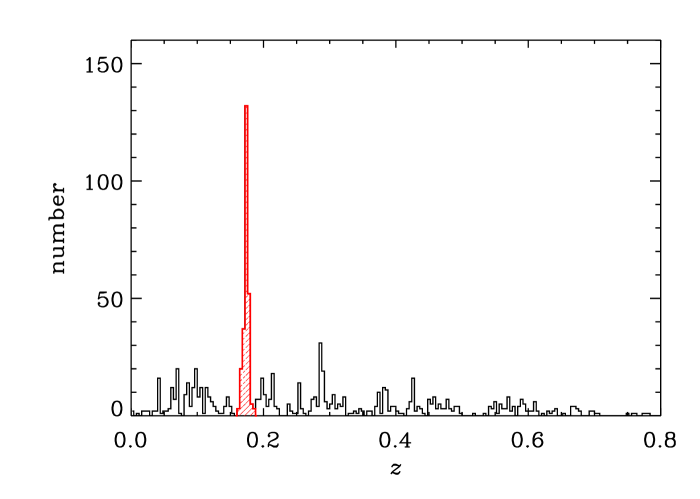
Figure 1: Histogram of redshifts in the cluster area. The red, hatched histogram shows galaxies with redshifts within $\pm 0.016$ of $\overline{z}=0.174$, the mean cluster redshift according to P07.

3 Cluster membership

To define which galaxies are members of the cluster we use their location in projected phase-space $R,v_{{\rm rf}}$, where $R$ is the projected (resp. 3D) radial distance from the cluster center (that we need to identify) and $v_{{\rm rf}}\equiv c\,(z-\overline{z})/(1+\overline{z})$, is the rest-frame velocity and $\overline{z}$ is the mean cluster redshift.

Following Beers et al. (1991) and Girardi et al. (1993) we first identify the cluster main peak in redshift space, by selecting the 252 galaxies with rest-frame velocities in the range $\pm 4000\,\mathrm{km\leavevmode\nobreak\ s}^{-1}$, that is within $\pm 0.016$ of the mean cluster redshift (see Fig. 1).

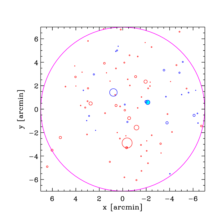
Figure 2: The positions of the cluster members with respect to the peak of their projected number density (the center is at $\alpha_{\mathrm{J2000}}=2^{\mathrm{h}}10^{\mathrm{m}}15\aas@@fstack{s}0,\;\delta_{\mathrm{J2000}}=-1\degr 2\arcmin 31\aas@@fstack{\prime\prime}$0). North is up and East is to the left. Galaxy positions are indicated by circles with sizes proportional to $1/(m_{R}-16.5)$, where $m_{R}$ are the galaxy red apparent magnitudes. Red (resp. blue) circles identify galaxies with $v_{{\rm rf}}\geq-677\,\mathrm{km\leavevmode\nobreak\ s}^{-1}$ (resp. $<-677\,\mathrm{km\leavevmode\nobreak\ s}^{-1}$), a limit that separates galaxies in the KMM-main subcluster from galaxies in the KMM-sub subcluster (see Fig. 6 in Sect. 4). The galaxy selected by D09 as the cluster center is indicated by a blue, cyan-filled, circle at $\{x,y\}=\{-2.1,0.7\}$. The purple circle has a radius of 1.24 Mpc and it indicates the cluster virial region (see text).

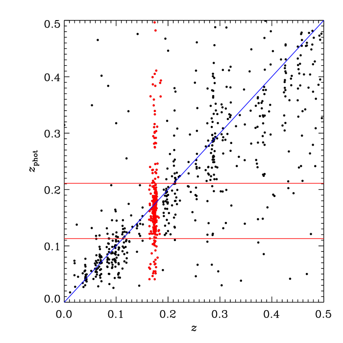
Figure 3: Photometric vs. spectroscopic redshift estimates for galaxies in the cluster area. Red dots identify galaxies in the main redshift peak of Fig. 1. The blue line represents the $z_{\mathrm{phot}}=z$ identity. The two horizontal red lines represent the $z_{\mathrm{phot}}$ limits that we adopt to define cluster members for galaxies without $z$.

To define the center of the cluster we cannot rely on the peak of the X-ray emission, because of poor photon statistics (D09). D09 noticed that the weak lensing peak of A315 was close to a local galaxy overdensity, and we chose the brightest galaxy of this overdensity as the cluster center. However, this galaxy does not appear to be the brightest cluster galaxy, as can be seen in Fig. 2. In this Figure we plot the cluster members (as defined below) as circles with sizes proportional to $1/(m_{R}-16.5)$, where $m_{R}$ are the galaxy red apparent magnitudes. Red (resp. blue) circles identify galaxies with $v_{{\rm rf}}\geq-621\,\mathrm{km\leavevmode\nobreak\ s}^{-1}$ (resp. $<-621\,\mathrm{km\leavevmode\nobreak\ s}^{-1}$), a limit that separates galaxies in the KMM-main subcluster from galaxies in the KMM-sub subcluster (see Fig. 6 in Sect. 4). The galaxy selected as the cluster center by D09 is part of the KMM-sub subcluster (that we identify in Sect. 4) and is not the brightest cluster galaxy in the central cluster region.

Since we can define the cluster center neither from its X-ray emission nor from the position of a dominant galaxy, we use as a center the peak of the projected number density of cluster galaxies, that we determine as follows. We consider the 2D projected spatial density distribution of cluster members, after correcting our spectroscopic sample for spatial incompleteness, since some regions are better covered by spectroscopic observations than others. To correct this sample for incompleteness, we rely on a sample with homogeneous spatial coverage, that is the sample of photometric members defined by using the photometric redshifts ($z_{\mathrm{phot}}$) from SDSS.

In Fig. 3 we show the correlation between $z_{\mathrm{phot}}$ and the spectroscopic redshift $z$, for the 913 galaxies which have both estimates (we restrict the plot to the redshift range 0–0.5). We follow Knobel et al. (2009) and select the $z_{\mathrm{phot}}$ range that minimizes the metric $\sqrt{(1-P)^{2}+(1-C)^{2}}$, where $P,C$ denote the purity and completeness of the photometric sample of selected members relative to the sample of 252 spectroscopic members selected in the main redshift peak. This metric reaches a minimum at $C=0.72,P=0.59$ for the $z_{\mathrm{phot}}$ range 0.113–0.211, a range we adopt to select 2327 photometric members.

Of all the selected photometric members, we only consider the 819 brighter than $z_{\mathrm{Petro}}\leq 19.64$ (corresponding to a luminosity $\simeq 0.13\,L^{\star}$, see Montero-Dorta & Prada 2009), a magnitude limit down to which the total number of galaxies with $z$ is $>1/4$ of the total number of galaxies with $z_{\mathrm{phot}}$. We determine the map of spectroscopic completeness by taking the ratio between the number of spectroscopic members and the number of photometric members in bins of RA, Dec. We then assign a completeness value to each galaxy in the spectroscopic sample and in the chosen magnitude range, according to the galaxy position.

We have 147 spectroscopic members with $z_{\mathrm{Petro}}\leq 19.64$ and with an assigned spectroscopic completeness $>1/4$, and we use this sample to construct an adaptive kernel map of the number density of galaxies in the cluster region, by weighting each galaxy by the inverse of its completeness value. The resulting map is shown in Fig. 4, and is centered on the point of maximum density, located at $\alpha_{\mathrm{J2000}}=2^{\mathrm{h}}10^{\mathrm{m}}15\aas@@fstack{s}0,\;\delta_{\mathrm{J2000}}=-1\degr 2\arcmin 31\aas@@fstack{\prime\prime}$0. This is the center we adopt for A315. Our adopted center is 0.39 Mpc away from the position adopted by D09, that was used as a center for the NFW (Navarro et al. 1997) profile fitting of the weak lensing map.

Once we have defined the cluster center, we can proceed to a better identification of the cluster members, by making use not only of the velocity of galaxies but also of their spatial distribution in the cluster region. We use the shifting-gapper (SG) algorithm of Fadda et al. (1996) to identify cluster members in projected phase-space, using a velocity gap size of 1000 $\mathrm{km\leavevmode\nobreak\ s}^{-1}$, a spatial bin size of 500 kpc, and a minimum of 15 galaxies per spatial bin, as indicated by Fadda et al. (1996). We identify 222 cluster members by this method, that is we reject 30 galaxies among those belonging to the main redshift peak. The location of the 222 selected members in the cluster area is shown in Fig. 4 and in projected phase-space in Fig. 5. Hereafter we refer to the sample of 222 cluster members as the ’Total’ sample.

We check our membership definition using the ’Clean’ algorithm of Mamon et al. (2013). Using the ’Clean’ algorithm the number of selected members is 208. Differences in the two member selection algorithms concern only galaxies located at distances $>1$ Mpc from the center. In the rest of the paper we present the results based on the SG membership selection, since the Clean algorithm is based on the assumption that the cluster mass profile follows a NFW distribution with a well defined theoretical mass-concentration relation. The SG algorithm is instead model-independent. Given that we investigate A315 because of its special properties, we want to avoid biasing the results by imposing typical characteristics of normal clusters. Anyway, we checked that the results of this paper are not significantly dependent on the choice of the membership algorithm.

The mean redshift and velocity dispersion of the cluster members, evaluated using the biweight (Beers et al. 1990), are $\overline{z}=0.1744\pm 0.0001,$ and $\sigma_{\rm{v}}=603_{-31}^{+29}\mathrm{km\leavevmode\nobreak\ s}^{-1}$ (see also Table 2). We use this estimate of $\sigma_{\rm{v}}$ to get a preliminary estimate of the cluster virial radius, $r_{200}$, that we denote $r_{200}^{\,\sigma}$. To estimate $r_{200}^{\,\sigma}$ we follow the iterative procedure of Mamon et al. (2013), where we assume an NFW model (Navarro et al. 1997) for the mass distribution, with a concentration given by the concentration–mass relation of Macciò et al. (2008), and we assume the Mamon & Łokas (2005) velocity anisotropy profile with a scale radius identical to that of the mass profile. We find $r_{200}^{\,\sigma}=1.24\pm 0.06$ Mpc. There are 89 members within $r_{200}^{\,\sigma}$.

4 Substructures

We consider the presence of substructures in the cluster by using the test of Dressler & Shectman (1988), modified as described in Appendix A. This test (DSb test hereafter) looks for local deviations of the mean velocity and velocity dispersion from the global cluster values. We apply the DSb test to the sample of cluster members defined in Sect. 3. In total, 17 members are flagged for their significant deviation in velocity from the local mean. Of these, 10 form a compact group in projection (see Fig. 4), that we call the ’DSb group’ hereafter. It has a mean velocity of $584\pm 95\,\mathrm{km\leavevmode\nobreak\ s}^{-1}$ in the cluster rest-frame, and a velocity dispersion of $282_{-58}^{+72}\,\mathrm{km\leavevmode\nobreak\ s}^{-1}$ (see also Table 2), typical of the general population of galaxy groups (see, e.g., Fig.3 in Ramella et al. 1999). The DSb substructure galaxies (including the DSb group) are displayed in the projected phase-space plot of Fig. 5.

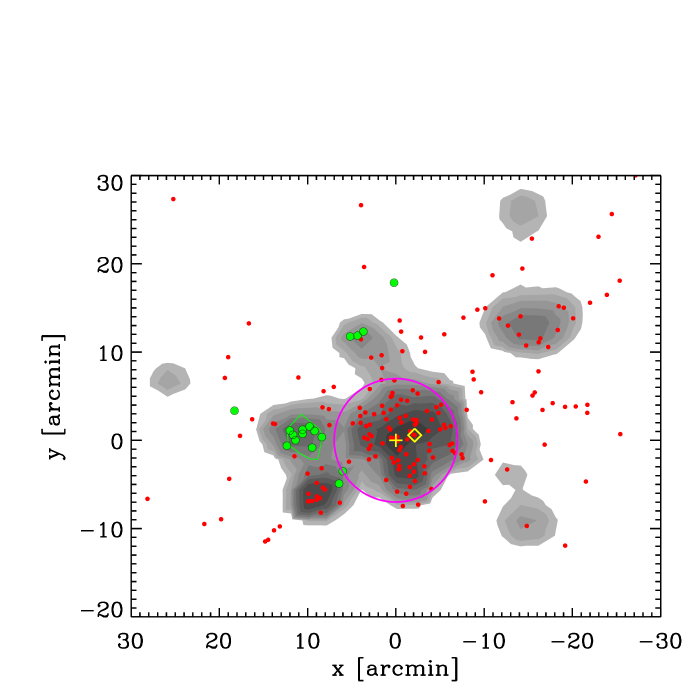
Figure 4: Adaptive-kernel map of the number density of cluster members with magnitude $z_{\mathrm{Petro}}\leq 19.64$, corrected for incompleteness of the spectroscopic sample. Darker shadings indicate higher densities, logarithmically spaced. The red dots identify all galaxies which are identified as cluster members by the SG algorithm (see Sect. 3). The green dots identify the galaxies flagged by the DSb procedure (described in Appendix A) as possible members of substructures. The green polygon indicates 10 of these galaxies that appear to form a compact group (the ’DSb group’). The map is centered at the point of maximum projected number density of cluster galaxies, as in Fig. 2 (also indicated by a yellow plus sign). North is up and East is to the left. The yellow diamond symbol identifies the position of the galaxy used as a cluster center in D09. The purple circle has a radius of 1.24 Mpc and indicates the cluster virial region (see Sect. 3).

After removing the 17 galaxies flagged by the DSb algorithm from the Total sample, we are left with 205 members, the ’No-DSb’ sample hereafter.

To investigate the presence of additional substructures that remain undetected by the DSb test, we apply the KMM algorithm (McLachlan & Basford 1988; Ashman et al. 1994) to the distribution of rest-frame velocities of the remaining 205 cluster members. The KMM algorithm fits a user-specified number of Gaussian distributions to a data-set, and returns the probability that the fit by many Gaussians is significantly better than the fit by a single Gaussian. Each Gaussian fit corresponds to a putative substructure of the cluster. The algorithm also returns the probability for each galaxy to belong to any of these substructures. Cluster velocity distributions are known to resemble Gaussians (e.g., Girardi et al. 1993), but not when substructures are present (e.g., Beers et al. 1991), in which case the decomposition of the velocity distribution into multiple Gaussians provides a more appropriate fit to the data (e.g., Boschin et al. 2008).

Table 2: Mean velocities and velocity dispersions

Sample	$N$	$\overline{v}$	$\sigma_{\rm{v}}$	TI
		$\mathrm{km\leavevmode\nobreak\ s}^{-1}$	$\mathrm{km\leavevmode\nobreak\ s}^{-1}$
Total	222	$0\pm 40$	$603_{-31}^{+29}$	1.07
DSb group	10	$584\pm 95$	$282_{-58}^{+72}$	–
No-DSb	205	$-60\pm 40$	$573_{-29}^{+28}$	1.05
Inner	88	$-205\pm 66$	$613_{-44}^{+48}$	0.88
KMM-main	63	$73\pm 56$	$441_{-38}^{+41}$	0.93
KMM-sub	25	$-924\pm 39$	$189_{-25}^{+29}$	0.94
Outer	117	$28\pm 46$	$503_{-32}^{+34}$	1.02

We consider the No-DSb sample, and the two subsamples of 88 members within $R\leq r_{200}^{\,\sigma}$and the 117 members outside (’Inner’ and ’Outer’ subsamples, hereafter). The KMM test indicates that the velocity distributions of both the No-DSb sample and the outer subsample are not significantly better fit with 2 Gaussians than with a single one. On the other hand, a 2-Gaussians fit to the velocity distribution of the inner subsample is significantly better than a single-Gaussian fit, with a probability of 0.05.

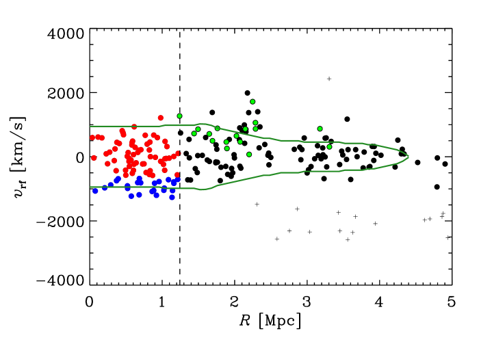
Figure 5: The projected phase-space distribution of galaxies in the cluster field, $v_{{\rm rf}}$ vs. $R$. Crosses and dots represent interlopers and cluster members, respectively, identified by the SG algorithm of Fadda et al. (1996). The vertical line is a preliminary estimate of the cluster $r_{200}$ ($r_{200}^{\,\sigma}$) based on the global estimate of the cluster velocity dispersion (see Sect.3). Members within $r_{200}^{\,\sigma}$ are identified with blue (resp. red) dots, if their probability to belong to the KMM-sub (resp. KMM-main) subclusters identified by the KMM algorithm (McLachlan & Basford 1988; Ashman et al. 1994) is $\geq 0.5$ (see text and Fig. 6). The green colored dots indicate those members that are flagged by the DSb procedure (described in Appendix A) as possible members of substructures. The green curves represent the Caustics identified by the Caustic technique of Diaferio & Geller (1997) (see Sect 5.2).

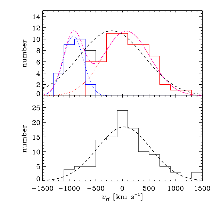
Figure 6: The velocity distribution of cluster members (after excluding galaxies flagged by the DSb substructure analysis). Top panel: members within $r_{200}^{\,\sigma}=1.24$ Mpc. The blue and red histograms identify the KMM partitions (namely, members with probability $\geq 0.5$ and, respectively, $<0.5$ to belong to the low-velocity group, KMM-sub). The dotted (blue and red) curves are the two Gaussians with mean and velocity dispersions obtained from the subsamples of the same colors. The dash-dotted magenta curve is the sum of the two Gaussians. The black dashed curve is the Gaussian with mean and velocity dispersion obtained from the full sample. Bottom panel: members outside $r_{200}^{\,\sigma}=1.24$ Mpc (histogram). The black dashed curve is the Gaussian with mean and velocity dispersion obtained from the full sample.

We show the velocity distribution of the inner subsample, separated according to the two KMM partitions, in the upper panel of Fig. 6, and the velocity distribution of the outer subsample in the lower panel of the same figure. We also show the Gaussians with averages and dispersions obtained from the biweight estimator (e.g., Beers et al. 1990) applied to the different distributions. In the projected phase-space plot of Fig. 5 we use red and blue dots to distinguish the two groups identified by the KMM algorithm in the inner sample.

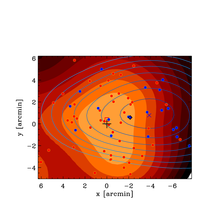
Figure 7: Adaptive-kernel maps of the number density of cluster members with magnitude $z_{\mathrm{Petro}}\leq 19.64$, corrected for incompleteness of the spectroscopic sample. Filled, red-orange contours represent the number densities of the KMM-main subcluster, open, blue-cyan contours represent the number densities of the KMM-sub one. The red square and blue X identify the density peaks of the KMM-main and KMM-sub density maps, resp. The contours are logarithmically spaced. The red (blue) dots identify member galaxies with velocity $>-621\,\mathrm{km\leavevmode\nobreak\ s}^{-1}$ (resp. $\leq-621\,\mathrm{km\leavevmode\nobreak\ s}^{-1}$) and are thus more (less) likely to belong to the KMM-main subcluster than to the KMM-sub one. The black cross identifies our adopted center of A315, from the analysis of the adaptive kernel density map of all members. The black diamond identifies the center used in D09.

In Fig. 7 we show the adaptive kernel density map of the galaxies in the two KMM groups – restricted to the virial region where the two groups are defined. As before, we use completeness weights to construct the map, and we only consider galaxies with $z_{\mathrm{Petro}}\leq 19.64$ and with an assigned spectroscopic completeness $>1/4$. We define the KMM-main and KMM-sub subclusters by considering galaxies of the inner subsample with $v_{{\rm rf}}\geq-621\,\mathrm{km\leavevmode\nobreak\ s}^{-1}$ and, respectively, and $v_{{\rm rf}}<-621\,\mathrm{km\leavevmode\nobreak\ s}^{-1}$, separated by the velocity value where the two best-fitting Gaussians intersect in Fig. 6. The density peak of the spatial distribution of the KMM-main subcluster is nearly coincident (0.07 Mpc separation) with our adopted center for the whole cluster, as expected given that 72% of the galaxies within $r_{200}^{\,\sigma}$ belong to the KMM-main subcluster. The center of the KMM-sub subcluster, on the other hand, is 0.7 Mpc to the West of the cluster center. The center used by D09 lies at intermediate distance along the line connecting the two group centers. The two groups overlap substantially in the projected spatial distribution, and this overlap is suggestive of a past or ongoing collision close to the line-of-sight.

In Table 2 we list the values of the average velocities $\overline{v}$ and velocity dispersions $\sigma_{\rm{v}}$, obtained with the biweight estimators, for the different samples considered so far. The removal of the galaxies flagged by the DSb substructure analysis does not affect the $\overline{v}$ and $\sigma_{\rm{v}}$ values of the whole cluster significantly. In particular, $\sigma_{\rm{v}}$ decreases by only 5% when we remove the 17 DSb-identified galaxies from the total sample. On the other hand, the $\sigma_{\rm{v}}$ of the Inner sample is significantly larger than those of the two groups into which it is split by the KMM algorithm (by 28% and 69%).

In the same Table we also list the values of the Tail Index ($TI$) of the velocity distribution in each sample (except the DSb group, since 10 members are not enough for a reliable estimate of $TI$). Beers et al. (1991) have suggested the use of $TI$ as a robust estimator of the shape of the velocity distribution in galaxy clusters. Values of $TI$ close to unity denote a Gaussian-like distribution, values $>1$ (resp. $<1$) a distribution with more (resp. less) galaxies at large velocity differences than expected for a Gaussian (leptokurtic and resp. platikurtic distribution). Popesso et al. (2007) have found that AXU clusters display on average a leptokurtic velocity distribution at large radii, with $TI=1.45$, and interpreted this evidence as suggestive of ongoing infall.

The values we find for the A315 cluster as a whole and for its different subsamples are not significantly different from unity, not even for the velocity distribution of members outside the virial region (see Table 2 in Bird & Beers 1993, for the significance levels of the $TI$). The velocity distribution within each KMM subcluster is closer to a Gaussian ($TI=0.93$ and 0.94) than the full velocity distribution in the virial region ($TI=0.88$). This difference of $TI$ values is not significant, but taken at face value it gives further support to the existence of two subclusters in velocity space. Had we not excluded the galaxies flagged by the DSb algorithm from our sample, the $TI$ value of the velocity distribution of the Outer sample would increase from 1.05 to 1.08, which is also not significantly different from unity.

5 The mass estimate

We proceed to estimate the mass of the cluster by two techniques, MAMPOSSt (Mamon et al. 2013) and the Caustic (Diaferio & Geller 1997). In these estimates, when needed, we take into account the results of the substructure analysis of Sect. 4. In particular, in MAMPOSSt we remove the galaxies flagged by the DSb technique, and we weigh galaxies by their probability of belonging to the KMM-main subcluster. In the Caustic method we use the KMM-main subcluster $\sigma_{\rm{v}}$ to select the relevant caustic.

5.1 MAMPOSSt

Figure 8: The Maximum Likelihood best-fit of a projected NFW model (Bartelmann 1996; Navarro et al. 1997) to the distribution of radial distances of the cluster members in the virial region and the binned number density profile with 1 $\sigma$ error bars. Only galaxies with $z_{\mathrm{Petro}}\leq 19.64$ and in regions of spectroscopic completeness $>1/4$ have been considered, and the sample has been corrected for incompleteness.

The MAMPOSSt technique has been developed by Mamon et al. (2013). It determines the best-fit parameters (and their uncertainties) of models for the mass and velocity anisotropy profile of a system of collisionless tracers in dynamical equilibrium in a spherical gravitational potential. To do so, it performs a Maximum Likelihood analysis of the projected phase-space distribution of the tracers, the member galaxies of the A315 cluster in our case. It has been tested with cluster-size halos extracted from cosmological simulations, by simulating a number of different observational situations.

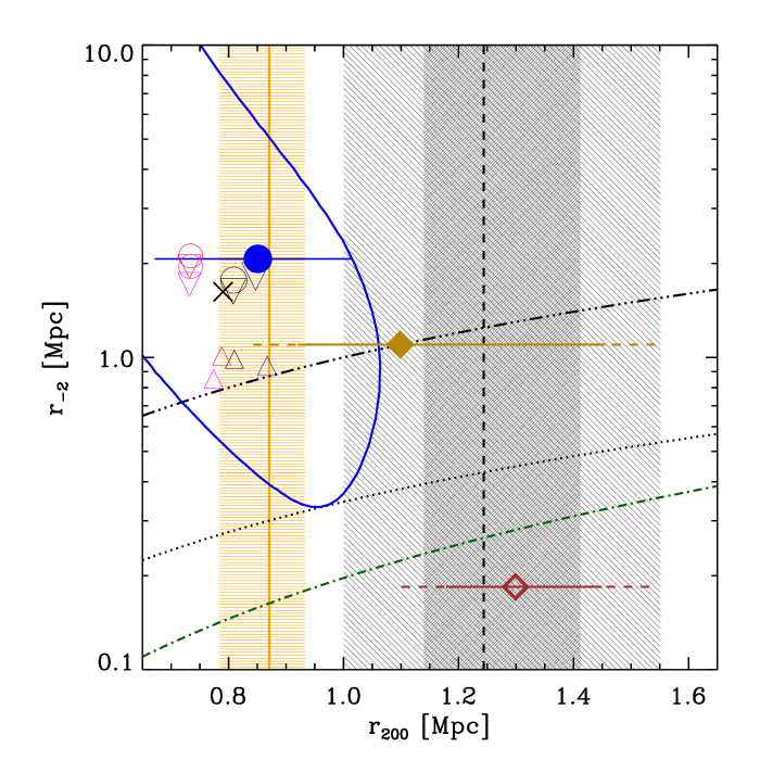
Figure 9: Results for the $M(r)$ parameters $r_{200}$ and $r_{-2}$. The blue contour indicates the 68% confidence level on the best-fit values obtained in MAMPOSSt (blue dot) for the best-fit models NFW+T (see text), after marginalization over the anisotropy parameter. The horizontal solid blue segment indicates the error on the best-fit $r_{200}$ value, obtained after marginalization over the $r_{-2}$ and the anisotropy parameter. The best-fit results of other models are indicated by the open symbols, triangle, inverted triangle, and circle, for the Bur, Her, NFW models, resp., black, red, magenta, and blue for the combination with the C, ML, OM, and T models, resp. The size of the symbols is proportional to the relative likelihood of the models. The black cross indicates the mean $[r_{200},r_{-2}]$, taking the average over all models. The vertical, black dashed line indicate the $r_{200}$ value obtained by D09 from their kinematic analysis. The uncertainties on this value, also taken from D09, are indicated by shaded grey regions, where the pale grey shading includes both the statistical and the systematic uncertainties, while the dark grey shading only includes the statistical uncertainty. The vertical orange line and orange shading indicate the $r_{200}$ value and uncertainty obtained from the cluster $L_{X}$ (from D09, ) using the scaling relation of Rykoff et al. (2008). The open maroon diamond indicates the $r_{200}$ value obtained by D09 from their lensing analysis. The position along the y-axis indicates the $r_{-2}$ value corresponding to the assumed concentration $r_{200}/r_{-2}$ used in D09 for the determination of the cluster lensing mass. The statistical and statistical+systematic uncertainties on this value are indicated by the maroon solid and dashed line, resp. The filled gold diamond indicates the new determination of $r_{200}$ from the lensing analysis applied to the same data used in D09, but this time using a concentration $r_{200}/r_{-2}=1$. This value of the concentration is used to set the position of the point along the y-axis. The dash-dotted green curve is the $r_{-2}$ vs. $r_{200}$ relation derived from the concentration-mass relation of Correa et al. (2015c) at the cluster redshift, computed with the code COMMAH (see also Correa et al. 2015a, b). The triple-dot-dashed black curve indicates the $r_{200}=r_{-2}$ relation. The dotted black curve indicates the $c_{200}=2.9$ relation, namely the highest concentration that is still marginally acceptable according to the MAMPOSSt dynamical analysis.

We use MAMPOSSt in the so called “Split” mode (see Sect. 3.4 in Mamon et al. 2013), that is we separate the maximum Likelihood analyses of the spatial and velocity distributions of member galaxies. We prefer to use MAMPOSSt in the Split mode since our spectroscopic sample suffers from spatially inhomogeneous incompleteness, and while this spatial incompleteness affects the determination of the number density profile, it is unlikely to affect the observational determination of the distribution of velocities.

To estimate the number density profile we consider the same subsample of spectroscopically selected members that we used to derive the adaptive kernel map (Fig. 4), restricted to the virial region, $R\leq r_{200}^{\,\sigma}$. We fit a projected NFW model (Bartelmann 1996; Navarro et al. 1997) to the distribution of radial distances with a Maximum Likelihood technique, weighting the galaxies by the inverse of their completeness times their probability of belonging to the KMM-main subcluster (see Sect. 4). This weighting scheme is to ensure that we are modeling the KMM-main subcluster density profile, rather than that of the whole Inner sample of members. The best-fit model is shown in Fig. 8. The best-fit NFW scale radius is $r_{\nu}=1.0_{-0.3}^{+0.7}$ Mpc. The uncertainties are large, but taking the result at face value it suggests a very low concentration of the galaxy distribution.

We then run MAMPOSSt on the Inner sample of members, by fixing the $r_{\nu}$ value at its best fit. We prefer to consider only galaxies within the expected virial region, to avoid including regions too far from virialization in the analysis. It has in fact been shown by Mamon et al. (2013) that $r_{200}$ is the optimal choice for minimizing the uncertainties in the parameter values obtained by MAMPOSSt. In calculating the likelihoods of the observed galaxy velocities, similarly to what we have done in the fit to the number density profile, we weigh each galaxy in the sample by its probability of belonging to the KMM-main subcluster. Weighing galaxies by their probabilities of belonging to the KMM-main subcluster is a way to account for the contamination by the KMM-sub subcluster, whose presumed members are assigned little (or zero) weight. We do not however use completeness as weights in the MAMPOSSt analysis, since the bias in the observational selection of spectroscopic targets can easily affect the spatial distribution, but not the velocity distribution of cluster members.

In MAMPOSSt we search for the best-fit values of three free parameters,

1. the virial radius $r_{200}$,

2. the scale radius of the mass distribution, that we choose to characterize by $r_{-2}$, the radius at which $\mathrm{d}\log\rho/\mathrm{d}\log r=-2$, where $\rho(r)$ is the mass density profile,

3. a parameter that characterizes the velocity anisotropy profile, $\beta(r)=1-\frac{\sigma_{\theta}^{2}(r)+\sigma_{\phi}^{2}(r)}{2\,\sigma_{r}^{2}(r)}=1-\frac{\sigma_{\theta}^{2}(r)}{\sigma_{r}^{2}(r)}$, where $\sigma_{\theta},\sigma_{\phi}$ are the two tangential components, and $\sigma_{r}$ the radial component, of the velocity dispersion, and we assume $\sigma_{\theta}=\sigma_{\phi}$.

We consider three models for the mass profile, $M(r)$: 1) Burkert (1995), 2) Hernquist (1990), and 3) Navarro et al. (1997) (Bur, Her, and NFW in the following). They are all characterized by two parameters, that we convert to $r_{200}$ and $r_{-2}$ when needed (see Biviano et al. 2013, for a detailed description of these models).

We consider four models for the velocity anisotropy profile, $\beta(r)$: 1) a model with constant anisotropy at all radii, that we denote ’C’, 2) the model of Mamon & Łokas (2005), that we denote ’ML’, 3) the model of Osipkov (1979) and Merritt (1985), that we denote ’OM’, and 4) the ’T’ model used in Biviano et al. (2013). Using four different models for $\beta(r)$ allows us to evaluate how much our results for $M(r)$ are dependent on the poorly known form of $\beta(r)$ in clusters of galaxies.

Table 3: MAMPOSSt results

Parameter	NFW+T models	Mean of all models
$r_{200}$ [Mpc]	$0.85_{-0.18}^{+0.16}$	$0.79\pm 0.02$
$r_{-2}$ [Mpc]	$2.1_{-1.0}^{+6.5}$	$1.6\pm 0.2$
$(\sigma_{r}/\sigma_{\theta})_{\infty}$	$0.7_{-0.3}^{+0.7}$	$0.8\pm 0.1$

The best-fit of MAMPOSSt is obtained for the combination of the NFW and T models. All other models are statistically acceptable, at better than the 68% confidence level. In Table 3 we give the best-fit values and uncertainties of $r_{200},r_{-2}$, and the anisotropy parameter, as well as the mean (and rms) of these same parameters, obtained by averaging over all the different model combinations. These values are also plotted in the plane of $r_{-2}$ vs. $r_{200}$ in Fig. 9. The variance of the values among different models is substantially smaller than the uncertainties in the best-fit model, indicating that the results are dominated by the statistical error, and the precise choice of the $M(r)$ and $\beta(r)$ models does not affect our conclusions.

The best-fit $r_{200}$ value found by MAMPOSSt, $r_{200}=0.85_{-0.18}^{+0.16}$, is significantly below our preliminary estimate, $r_{200}^{\,\sigma}=1.24\pm 0.06$ Mpc. This difference is due to the fact that here we adopt a weighting scheme that effectively forces MAMPOSSt to consider mostly (if not only) the velocities of the members of the KMM-main subcluster, while the $r_{200}^{\,\sigma}$ value was derived from the $\sigma_{\rm{v}}$ estimated using the velocity distribution of all the cluster members. We repeat our $\sigma_{\rm{v}}$-based estimate of the virial radius by considering only those galaxies with a probability $\geq 0.5$ of belonging to the KMM-main subcluster. We find $r_{200}^{\,\sigma}=0.90\pm 0.09$ Mpc, fully consistent with the MAMPOSSt result. For comparison, the corresponding value for the KMM-sub subcluster is $0.38\pm 0.05$ Mpc.

The uncertainty on the MAMPOSSt value of $r_{200}$ is much larger than that on $r_{200}^{\,\sigma}$. This difference seems strange, given that MAMPOSSt uses the full velocity distribution, and not only its $2^{nd}$ moment. The fact is, the uncertainty in the $\sigma_{\rm{v}}$-based estimate ($r_{200}^{\,\sigma}$) is obtained by assuming knowledge of $M(r)$ and $\beta(r)$. The larger uncertainty of the MAMPOSSt $r_{200}$ estimate is more realistic, as in the MAMPOSSt procedure we allowed for a much wider range of $M(r)$ and $\beta(r)$ models and parameters.

The best-fit $r_{-2}$ value obtained by MAMPOSSt is surprisingly larger than the $r_{200}$ value, implying a concentration $c_{200}\equiv r_{200}/r_{-2}<1$, at odds with theoretical expectations (e.g., Bhattacharya et al. 2013; De Boni et al. 2013). We show in Fig. 9 that the expected theoretical value of $r_{-2}$ for a cluster this massive at this redshift is $\lesssim 0.2$ (we use the COMMAH routine by Correa et al. 2015a, b, c, for this estimate). Hence the concentration we find is almost an order of magnitude smaller than expected.

The anisotropy parameter $(\sigma_{r}/\sigma_{\theta})_{\infty}$ has a best-fit value below unity, characteristic of tangential orbits, but with large error bars that do not rule out isotropic or even radial orbits. Tangential orbits are not commonly seen for cluster galaxies (Biviano & Poggianti 2009; Wojtak & Łokas 2010; Biviano et al. 2013), but they seem to be more common in clusters with subclusters (Biviano & Katgert 2004; Munari et al. 2014).

5.2 Caustic

The Caustic method has been developed by Diaferio & Geller (1997), and Diaferio (1999) and is a rather simple way to determine the mass profile of galaxy clusters from the amplitude of the galaxy velocity distribution at different distances from the cluster center. In practice, one estimates the density of galaxies in projected phase-space, and define iso-density contours. The iso-density contour that defines ’the Caustic’ is chosen by comparing the square amplitude in velocity space, weighted by the local density of galaxies, to the $\sigma_{\rm{v}}$ of cluster members in the virial region. The Caustic method is supposed to work independently of the presence of substructures, and does not require the identification of cluster members, if not for the purpose of estimating the cluster $\sigma_{\rm{v}}$ in the virial region. Here we determine the Caustic by using all galaxies with redshifts in the cluster region (not only members, and including galaxies in substructures), but fixing the cluster $\sigma_{\rm{v}}$ to the value found for the KMM-main subcluster (see Table 2). The Caustic found is shown in Fig. 5.

To convert the Caustic amplitude (along the velocity axis) into a mass estimate for the cluster, we need to choose a value for the filling factor ${\cal F}_{\beta}$ (see Diaferio 1999, for its definition). Several values have been used so far, ranging from 0.5 to 0.7 (Diaferio & Geller 1997; Serra et al. 2011; Geller et al. 2013; Gifford et al. 2013). Using ${\cal F}_{\beta}=\{0.5,0.7\}$ we find $r_{200}=0.9_{-0.6}^{+0.3}$ Mpc, and $1.0_{-0.6}^{+0.4}$ Mpc, respectively, where the uncertainties are evaluated following the prescriptions of Diaferio (1999). Clearly, the statistical error dominates over the systematic uncertainty in the value of ${\cal F}_{\beta}$.

The Caustic analysis provides very poor constraints on $r_{200}$ (and therefore the cluster mass), but taken at face value they are close to those obtained with MAMPOSSt (Sect. 5.1) in particular for ${\cal F}_{\beta}=0.5$.

6 Discussion

Table 4: $M_{200}$ estimates

Method	$M_{200}$	Reference
	[$10^{14}\,M_{\odot}$]
Lensing	$3.0_{-0.8-0.5}^{+1.2+0.7}$	D09
Virial	$2.7_{-0.7}^{+1.1}\pm 1.0$	D09
$L_{X}$	$0.9_{-0.2}^{+0.2}$	D09
MAMPOSSt	$0.8_{-0.7}^{+0.8}$	This paper
Caustic ${\cal F}_{\beta}=0.5$	$0.9_{-0.9}^{+1.4}$	This paper
Caustic ${\cal F}_{\beta}=0.7$	$1.5_{-1.4}^{+2.4}$	This paper
Lensing with $c_{200}=1$	$1.8_{-0.9}^{+1.7}$	This paper

In Table 4 we list the cluster $M_{200}$ values found in this paper and in D09. Both statistical and systematic errors are given for the mass estimates of D09. For the MAMPOSSt mass estimates, the listed errors include the systematics related to the unknown mass and velocity anisotropy distributions, since our choice of $M(r)$ and $\beta(r)$ models has not been restrictive. As for the Caustic mass estimates, the systematic error is dominated by the choice of ${\cal F}_{\beta}$, for which we have considered the two extreme values generally adopted in the literature.

Our new kinematic estimates of $M_{200}$ are in agreement with the one obtained from the cluster $L_{X}$ using the scaling relation of Rykoff et al. (2008). On the other hand, our new estimates are substantially below (by a factor $\sim 3$) the one obtained by the kinematic analysis of D09 which was based on a sample of 25 cluster members.

Numerical simulations indicate that a bias $>2$ is not unexpected in kinematic mass estimates based on only $\sim 20$ spectroscopic members, as it occurs in 25% of the cases (Biviano et al. 2006). In these simulations, the presence of substructures along the line-of-sight was identified as the main cause of a large bias in the mass estimate (Biviano et al. 2006). While we could not identify any sign of subclustering in A315 with a sample of only 25 members, thanks to our extensive spectroscopic campaign, we have now been able to detect one small group in the external cluster regions, and, most importantly, a distinct bimodality in velocity space in the inner cluster region. This bimodality is due to two subclusters with an overlapping spatial distribution that suggests they are colliding or have collided close to the line-of-sight. The $r_{200}^{\,\sigma}$ estimates of the KMM-main and KMM-sub subclusters imply a mass ratio of $\sim 0.1$. Adding the KMM-sub $M_{200}$ to the total cluster mass estimate therefore does not change our conclusion that our previous kinematic mass estimate of A315 has been grossly overestimated.

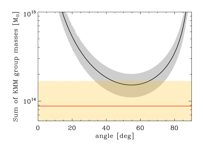
Figure 10: The black line shows the requirement for the two KMM subclusters to be gravitationally bound, as computed from the Newtonian criterion; the grey shading indicates 1 $\sigma$ uncertainties on this requirement, which depends on the projected distance and line-of-sight velocity difference of the two subclusters. The red line indicates the sum of the measured masses for these subclusters; the orange shading indicates 1 $\sigma$ uncertainties on this sum. On the x-axis, the angle between the axis connecting the KMM-main and KMM-sub subclusters is defined with respect to the plane of the sky (90 degrees corresponds to a line-of-sight collision). The KMM subclusters are gravitationally bound for an angle between $\sim 35$ and $\sim 75$ degrees, if we take into account both the uncertainties on our mass estimates and the uncertainties on the Newton criterion requirements.

If the two subclusters are physically unrelated, and their velocity difference attributed to different Hubble flows, the smallest subcluster would lie $\sim 18$ Mpc in the foreground. However, the subclusters are unlikely to be completely unrelated, as we can see by applying the Newtonian criterion for gravitational binding of the two subclusters (eq.(5) in Beers et al. 1991). To apply the Newtonian criterionwe use the difference in the subcluster mean line-of-sight velocities ($851\pm 68\,\mathrm{km\leavevmode\nobreak\ s}^{-1}$), and the projected separation between their centers ($0.66\pm 0.10$ Mpc). We use the MAMPOSSt $M_{200}$ estimate for the KMM-main subcluster (see Table 4) and 1/10 of this same estimate for the KMM-sub subcluster. The result is shown in Fig. 10 and indicates that a bound solution is acceptable within the observational uncertainties, for a wide range of values of the angle between the collision axis and the plane of the sky. The bound solution is even more likely than our estimate indicates, because we have used $M_{200}$ masses, and these do not account for the additional mass within the infall regions of the two subclusters (the total mass of the system would increase by a factor $\sim 2$; Rines et al. 2013).

The bound solution does not inform us on whether the two subclusters are observed before or after their collision. A past collision between the two subclusters might be invoked to explain the very low concentration ($c_{200}<1$) observed both for the galaxy and the mass distribution of the main component of A315. Such a low concentration is indeed uncommon (Lin et al. 2004; Budzynski et al. 2012) and theoretically unexpected (e.g., Correa et al. 2015c). Observationally, it has been shown that the radial distribution of galaxies in clusters with substructures is less concentrated than that of galaxies in relaxed clusters (Biviano et al. 2002). On the theoretical side, numerical simulations have shown that the scale radius of the mass distribution increases after a merger (Hoffman et al. 2007). A low-concentration of the mass distribution characterizes not fully virialized clusters (Jing 2000; Neto et al. 2007).

Could then the low concentration we observe originate from the collision with the subcluster identified by the KMM analysis? To answer this question, we estimate the probability of a halo of mass similar to the mass of A315, to have a concentration $c_{200}<2.9$. This is the highest value that is still marginally acceptable according to our MAMPOSSt dynamical analysis of A315 (dotted curve in Fig, 9). We use the concentration distributions of the halos in the Millennium Simulation derived by Neto et al. (2007). More precisely, we consider the lognormal best-fit models listed in their Table 1, for the halos in the mass range closest to our A315 mass estimate. While only 1% of relaxed halos have $c_{200}<2.9$, 28% of unrelaxed halos have such a low concentration or lower. This fraction drops to 0.005% at $c_{200}<1$. It then appears that the best-fit concentration value we observe is rarely observed in cosmological simulated halos, but not when we account for the observational uncertainties and for the unrelaxed nature of A315.

The low-concentration of the mass distribution of A315 might also account for part of the mass overestimate from lensing (D09). D09 treated the NFW profile as a 1-parameter profile where the concentration follows the theoretical mass-concentration relation of Dolag et al. (2004) exactly. At the best fit $M_{200}$ in D09 the concentration used was 7.0. Performing a two-parameter fit, with a free concentration parameter is unfortunately not allowed by the quality of the D09 data. In particular, the low total number of galaxies inside the NFW scale radius limits the constraining power of this data set. Furthermore, contamination of the catalog of lensed galaxies by cluster galaxies dilutes the shear signal in a radially-dependent way that is extremely challenging to model even for much better quality data than those of D09. We therefore repeat the weak lensing analysis of D09 on the same data and with the same technique, but this time forcing $c_{200}=1$ instead. We obtain $M_{200}=1.8_{-0.9}^{+1.7}\times 10^{14}M_{\odot}$, that brings the lensing mass estimate in agreement with the kinematic and X-ray estimates within 1 $\sigma$ (see Fig. 9 and Table 4).

In addition, the lensing mass estimate might be further reduced by considering that it is derived assuming a spherical NFW profile, while the cluster mass distribution is elongated along the line-of-sight due to the two overlapping subclusters (e.g., Corless & King 2007; Dietrich et al. 2014). If the elongation is only due to the superposition of the two subclusters, we expect the effective axis ratio of the total mass distribution not to be too far from unity. However, in low concentration clusters, the mass ratio between the best-fitting lensing mass obtained assuming a spherical NFW halo and the true mass of an elliptical NFW halo, can be $\sim 1.1$ also for a relatively small axis ratio (see Fig. 2 in Dietrich et al. 2014).

Due to its dependence on the square of the electron density, X-ray luminosity-based mass estimates are to a good approximation not affected by triaxiality. However, the low mass concentration suggests that A315 might be a non-cool-core cluster. The mass estimate that one obtains from $L_{X}$ via a scaling relation obtained for an unbiased cluster sample, is systematically lower for non-cool-core clusters, by $\sim 25$% (see Fig. 3 in Zhang et al. 2011). Indeed, scaling relations with core-excised $L_{X}$ have less dispersion and lower systematics than those obtained from the total $L_{X}$ (Mittal et al. 2011).

The presence of substructure in the velocity distribution of A315 and its low mass concentration, thus seems to be able to reconcile the X-ray, lensing, and kinematic cluster mass estimates. Possibly the presence of substructures and the low mass concentration are both the manifestation of the same phenomenon, namely a collision along the line-of-sight of a poor cluster and a galaxy group.

In conclusion, our new analysis rules out the X-ray underluminous nature of A315, just as it was done for A1456 by D09. These clusters appear X-ray underluminous because their velocity dispersions are inflated by infalling, unrelaxed halos – an interpretation originally given by Bower et al. (1997) to explain the existence of low-$L_{X}$ clusters with high $\sigma_{\rm{v}}$.

A315 and A1456 are however only 2 of 51 AXU clusters in the sample of P07. Both were found to be characterized by a bimodal velocity distribution when analyzed in detail and with more spectroscopic data (in the case of A315). Such a velocity distribution is characterized by low $TI$ values (like the one we obtain for the Inner sample of A315, see Table 2), as expected from the presence of two kinematically distinct components with a mean velocity offset (see, e.g., the case of A85 in the study of Beers et al. 1991). However, low $TI$ values are not typical of AXU clusters, that P07 found instead to have velocity distributions characterized by high $TI$ values outside the virial region, a feature that remains to be explained. One possibility is that high $TI$ values are caused by the presence of high-velocity interlopers that are not removed by the membership selection procedure, which could fail for poor statistical samples. More detailed investigations of other AXU clusters are needed before we can dismiss the existence of intrinsically X-ray underluminous clusters altogether.

7 Conclusions

We re-determine the kinematic mass estimate of the $z=0.174$ cluster A315, which had previously been identified as being X-ray underluminous for its kinematic and lensing mass (; ). Our new kinematic estimate is based on redshifts for $\sim 200$ cluster members, in part obtained through our new spectroscopic observations with VIMOS at the VLT. These are the results of our analysis:

• We identify previously undetected substructures. In particular, the velocity distribution of cluster members in the virial region displays a significant bimodality, caused by the projection of two distinct subclusters along the line-of-sight.

• Accounting for these substructures in our kinematic analysis (conducted via MAMPOSSt and the Caustic method, Mamon et al. 2013; Diaferio & Geller 1997, resp.), leads to a substantial and significant reduction of the kinematic mass estimate of D09, which was based on 25 members only. Our kinematic mass estimate, $0.8_{-0.4}^{+0.6}\times 10^{14}M_{\odot}$, is in agreement with the estimate that we obtain from the cluster $L_{X}$ through the scaling relation of Rykoff et al. (2008), $0.9\pm 0.2\times 10^{14}M_{\odot}$.

• In our dynamical analysis we also determine the cluster mass concentration. We find $c_{200}<1$, an unusually low value. We argue that this is the effect of a $\sim 1$:10 mass-ratio collision between the two subclusters identified in the virial region.

• Using our estimate of $c_{200}$, we redetermine the weak lensing mass of A315 using the same method of D09, and we find $M_{200}=1.8_{-0.9}^{+1.7}\,M_{\odot}$. This mass estimate is 40% lower than the estimate of D09, which was obtained using a much higher concentration, inferred from a theoretical concentration-mass relation. Accounting for elongation of the cluster along the line-of-sight could further reduce our new lensing mass estimate (by $\gtrsim 10$%).

• The low-mass concentration we find might suggest that A315 is not a cool-core cluster. Its $L_{X}$ might therefore correspond to a slightly higher mass (by $\sim 25$%) than the one predicted by the Rykoff et al. (2008) scaling relation.

Our new results dismiss the AXU nature of A315, just as it was done for A1456 by D09. The A315 $L_{X}$ no longer appears too low for its mass. Its lensing mass had been over-estimated because it was derived assuming a normal mass concentration, rather than the true, very small one. The cluster kinematic mass had previously been over-estimated because of an undetected bimodality in its velocity distributions. This was also the case of A1456. Both clusters belong to the category of systems whose velocity dispersions are inflated by infalling subclusters or groups projected along the line-of-sight (Bower et al. 1997). Whether line-of-sight projections are the only explanation for the nature of AXU clusters is impossible to say before more candidates are examined with the same level of detail used for A315. These studies will help quantifying the biases in cluster mass estimates, a fundamental issue for the use of clusters as cosmological probes.

Appendix A The modified Dressler & Shectman (DSb) test

The original version of the test looked for these deviations in all possible groups of 11 neighboring galaxies identified within a cluster (Dressler & Shectman 1988). Biviano et al. (1996, see Appendix A.3 in that paper) adapted this method to make adaptive-kernel maps of the quantity $\delta$ that describes the average velocity and velocity dispersion deviation from the global cluster value. Biviano et al. (2002) then modified $\delta$ into its two components $\delta_{v}$ and $\delta_{\sigma}$, that separately measure the local deviations of the average velocity and velocity dispersion, respectively. They also introduced the use of the velocity dispersion profile, in lieu of the total cluster velocity dispersion, as a reference value for $\delta_{\sigma}$.

Figure 11: The cluster projected velocity dispersion profile, normalized by the total velocity dispersion (dots with 1 $\sigma$ error bars). The solid curve represent the smoothed profile, adopted in the Dressler & Shectman test. The dashed curve shows, for comparison, the smoothed profile obtained for a sample of nearby clusters by Biviano et al. (2002).

We combine the modifications proposed by Biviano et al. (1996) and Biviano et al. (2002). Specifically, we evaluate the local values of mean velocity and velocity dispersion by constructing weighted adaptive-kernel density maps of cluster members, with the weights given by $v$ and $v^{2}$, and dividing these maps by the unweighted adaptive-kernel number density map of cluster members,

$$\delta_{v}(\@vec{x})=\sum_{j=1}^{N}K_{j}^{(2D)}(\@vec{x})v_{j}/\sum_{j=1}^{N}K_{j}^{(2D)}(\@vec{x})$$ (1)

$$\delta_{\sigma}(\@vec{x})=[\sum_{j=1}^{N}K_{j}^{(2D)}(\@vec{x})v^{2}_{j}/\sum_{j=1}^{N}K_{j}^{(2D)}(\@vec{x})]^{1/2}-\sigma_{v}(R)$$ (2)

where $K_{j}^{(2D)}(\@vec{x})$ is the 2D kernel at the position $\@vec{x}$, and $\sigma_{v}(R)$ is the total cluster velocity dispersion profile, that is the velocity dispersion at a given projected position $R$, shown in Fig. 11.

The significance of the $\delta_{v}$ and $\delta_{\sigma}$ at any position $\@vec{x}$ are evaluated separately, by bootstrap resamplings (Efron & Tibshirani 1986).