LHCb trigger streams optimization

Abstract

The LHCb experiment stores around $10^{11}$ collision events per year. A typical physics analysis deals with a final sample of up to $10^{7}$ events. Event preselection algorithms (lines) are used for data reduction. Since the data are stored in a format that requires sequential access, the lines are grouped into several output file streams, in order to increase the efficiency of user analysis jobs that read these data. The scheme efficiency heavily depends on the stream composition. By putting similar lines together and balancing the stream sizes it is possible to reduce the overhead. We present a method for finding an optimal stream composition. The method is applied to a part of the LHCb data (Turbo stream) on the stage where it is prepared for user physics analysis. This results in an expected improvement of 15% in the speed of user analysis jobs, and will be applied on data to be recorded in 2017.

1 Introduction

To capture and analyze a large number of collision events, the LHCb experiment [1] relies on a multi stage data processing pipeline [2]. The events are filtered through the hardware L0 trigger and two levels of software triggers – HLT1 and HLT2. Physicists develop algorithms (called lines) that select particular types of events that they wish to study. All the events that satisfy the requirements of at least one HLT2 selection line are permanently recorded to tape storage. Since Run-II, the HLT2 output data have been split into two streams. Data in the FULL stream need to be reconstructed on distributed computing resources and are intended for further event selection, before being made available for user analysis. Run-II saw the introduction of the Turbo stream, with a event format ready for analysis right after the trigger step, without further event preselection. Turbo stream data are prepared for physics analysis by an application called Tesla [3].

User analysis jobs run independently and usually require only a small subset of all events selected by the lines. Efficient data storage and access methods are therefore required. LHCb uses the Worldwide LHC Computing Grid (WLCG), which supports data granularity on file level [4].

The LHCb experiment uses two factors to group events into files. First, a file only contains events from a single run. In LHCb a run corresponds to a period of up to 1 hour of data taking, in which the beam and detector conditions are presumed constant. This makes it easier to apply different collision conditions and discard runs that are flagged up by the data quality assessment. Second, the lines are grouped into streams, such that each file available for user analysis corresponds to a particular run-stream pair. If an event passes lines from different streams, it (wholly or partially) will be copied to multiple files. Sets of files corresponding to particular streams are themselves also called streams [5]. Both FULL and Turbo stream are further divided into streams. To avoid confusion in this paper we refer to the streams into which the Turbo stream is divided as Tesla streams.

2 Optimization criteria

Several considerations are made when defining the mapping of lines to streams.

• User job performance. A job has to read a whole Tesla stream even if it needs only a small subset of events in it. The optimum is achieved if each line is assigned to a separate stream. For Tesla streams, the estimated time spent by the user jobs on disk access differs by a factor of 5 between the extreme variants. The metric is described in Sect. 2.1 and 4.2.

• Storage space. Information is duplicated when an event belongs to multiple streams. The optimal storage performance would be achieved if all lines belong to a single stream. For Tesla streams, the scheme where each line is assigned to a separate stream will take 1.5x more space than a single stream. The evaluation procedure for storage space usage is described in Sect. 4.1.

These factors must be estimated in order to construct a streaming scheme. There is another constraint — WLCG often uses tape storage systems, which generally do not cope well with storing and providing frequent access to many small files [6]. Since each stream has at least one file for each run, the number of files grows with the number of streams. The other problem is the management of those streams for the data management team. More streams need more operations on them (replication, deletion, also staging).

2.1 Disk access time

The total time spent by user jobs on disk access depends on two independent factors: the queries the users make and the time it takes to complete each query. We use the following assumptions:

• The number of times each event is requested is proportional to the number of lines it passes.

• The time that a job would spend on disk access is proportional to the number of events in the stream that the job reads.

So the total time would be proportional to

$$T=\sum_{\text{streams}}N_{\text{events in stream}}\cdot N_{\text{lines in stream}}$$ (1)

Some lines are prescaled – line positive selection decisions are randomly discarded with a specified probability. This can be accommodated by using the expected value of $T$:

$$E\left(T\right)=\sum_{\text{streams}}N_{\text{lines in stream}}\cdot E\left(N_{\text{events in stream}}\right),$$ (2)

$$E[N_{\text{events in stream}}]=\sum_{e}\left(1-\prod_{l}\left(1-\Delta_{el}P_{l}L_{ls}\right)\right),$$ (3)

where $\Delta_{el}\in\{0,1\}$ is the indicator whether event $e$ passes line $l$, $P_{l}\in[0,1]$ is line $l$ prescale value, $L_{ls}\in\{0,1\}$ is the indicator whether line $l$ belongs to stream $s$.

2.2 Disk usage

The amount of information about an event recorded to a particular stream has a non-trivial relationship with the set of lines from that stream that have selected the event. We use a simplified model in which there are 2 types of Turbo lines. Pure Turbo lines store the information about the decay candidate that triggers the selection of the event. These are assumed to have a size of $10$ kB per line. In 2016, the Turbo stream was extended to allow full event reconstruction information to be persisted. These lines with the PersistReco flag are assumed to store an additional $50$ kB shared among such lines. Thus, the formula for event $e$ size $S_{es}$ in the stream $s$:

$$S_{es}=10\cdot N_{\text{turbo lines}}+50\cdot I_{\text{persist reco}}$$ (4)

where $N_{\text{turbo lines}}\in\mathbf{N}_{0}$ is the number of lines with the Turbo flag belonging to the stream $s$ that the event passes, $I_{\text{persist reco}}\in\{0,1\}$ is the indicator of whether the event passes a line with the PersistReco flag belonging to the stream.

3 Optimization

This is a clustering problem – we want lines that select similar events to be grouped together. We have tried classic clustering algorithms from scikit-learn [7]: KMeans, SpectralClustering, Birch, AffinityPropagation. They have failed to improve the baseline, which is not surprising given that the loss functions used are quite different from ours. We therefore postulate that our algorithm must

• optimize $T$ directly instead of some cluster goodness function

• allow for different cost functions to be able to utilize a more accurate model in the future

• converge to a reasonable solution within a reasonable time

• accept the number of streams as a parameter to maintain the WLCG constraint on the number of files

3.1 Continuous loss

The first step is the transition from discrete to continuous optimization to be able to use fast gradient methods. Instead of assigning the lines to streams, we let each line $l$ have a probability $\tilde{L}_{ls}$ to be in each stream $s$.

$$E\left[N_{\text{lines in stream}}\right]=\sum_{l}\tilde{L}_{ls},$$ (5)

$$E\left[N_{\text{events in stream }s}\right]=\sum_{e}\left(1-\prod_{l}\left(1-\Delta_{el}P_{l}\tilde{L}_{ls}\right)\right).$$ (6)

After optimization, we assign each line to the stream with the highest probability of containing it.

$$\tilde{T}=\sum_{s}E\left[N_{\text{lines in stream }s}\right]\cdot E\left[N_{\text{events in stream }s}\right]$$ (7)

$$=\sum_{s}\left[\sum_{l}\tilde{L}_{ls}\cdot\sum_{e}\left(1-\prod_{l}\left(1-\Delta_{el}P_{l}\tilde{L}_{ls}\right)\right)\right].$$ (8)

In general, $\tilde{T}\neq E[T]$. However, if all the assignments are definite, $L_{ls}\in\{0,1\}$ and $\tilde{T}=T$. In practice on our data, the algorithm has nearly always converged to near integer probabilities.

3.2 Solving the boundary conditions

Since $\tilde{L}_{ls}$ are probabilities, there are constraints on their values:

• $\tilde{L}_{ls}\in[0,1]$

• the sum of the probabilities of all random outcomes must be 1, $\sum_{s}\tilde{L}_{ls}=1$

To satisfy these conditions, we have parametrized $\tilde{L}_{ls}$ with softmax [8]:

$$\tilde{L}_{ls}=\frac{e^{A_{ls}}}{\sum_{s}e^{A_{ls}}},$$ (9)

$A_{ls}$ can have any value.

3.3 Grouping constraints

Line usage is not independent. Some lines are often requested together. Therefore, from the point of view of user convenience, it is desirable to have those lines in a single stream. From now on, such groups will be referred to as modules.

The formula for $\tilde{T}$ can be parametrized to make the result strictly adhere to the grouping requirement:

$$\tilde{\Delta}_{em}=1-\prod_{l}\left(1-\Delta_{el}P_{l}M_{lm}\right),$$ (10)

$$\tilde{\tilde{T}}=\sum_{s}\left[\left(\sum_{m}\sum_{l}M_{lm}\tilde{L}_{ms}\right)\cdot\sum_{e}\left(1-\prod_{m}\left(1-\tilde{\Delta}_{em}\tilde{L}_{ms}\right)\right)\right],$$ (11)

where $M_{lm}\in\{0,1\}$ is the indicator of whether the module $m$ contains the line $l$, $\tilde{L}_{ms}$ is the probability of module $m$ being in stream $s$, $\tilde{\Delta}_{em}$ is the probability that event $e$ was selected by the module $m$.

3.4 Implementation

The optimization is implemented in Python using the theano framework [9]. Theano is a mature framework primarily used for deep learning. Its major advantages for our task are speed and symbolic gradients computation. We have tested several gradient optimization algorithms: Nesterov Momentum, AdaMax, AdaGrad, AdaM, AdaDelta, AdaMax. For our data the best results are achieved with AdaMax.

The code is freely available under Apache License 2.0: https://gitlab.cern.ch/YSDA/streams-optimization/

4 Results for the LHCb Turbo stream

The method is applied to find an optimal Tesla stream composition for the LHCb Turbo stream. We take a sample of $10^{5}$ Run-II Turbo events recorded in October 2016 and compare the optimized streams to the baseline where the lines are grouped by physical similarity [10].

HLT lines are grouped into separate modules that are typically authored by a small team. They tend to contain several selections that are topologically similar and/or are required for a single analysis or set of related analyses. One of the modules contains several hundred selections of charm hadron decay selections. This module is divided into submodules. For user convenience, we do not split the modules and charm hadron submodules.

4.1 Model validation

We stream the events with various streaming schemes – produced by our algorithm for different stream numbers and the baseline. We measure the files sizes and the time needed to process the files with a minimalist analysis job using the DaVinci application [11], which only reads events and lists HLT decision flags in them. For each stream in each scheme, we calculate the $T$ and $S$ values and calibrate them by fitting a least squares linear regression. For the calibrated values, we compute the coefficient of determination. The results are as follows:

$$R^{2}(T)=0.57,$$ (12)

$$R^{2}(S)=0.98.$$ (13)

The model is good in describing event sizes. For reading times, the model is not perfect. It appears that the time it takes to read an event depends on the event structure.

Job run time on a real world computer is subject to random fluctuations. To estimate their influence, we rerun the DaVinci job 5 times. The standard deviation of the results is 2%.

4.2 Results

We build optimized schemes for different numbers of streams. Then we stream the events and, for each resulting file, measure size and reading time $T_{\text{stream}}$. The difference in total file sizes is less than 2%. For the reading times, we apply the same query assumptions we used in our model – the number of times each event is requested is proportional to the number of lines it passes. The test job also takes some time to initialize – $T_{\text{initial}}\approx 9\ \text{s}$. This is a function of the job and not of the streaming scheme, and is accounted for.

$$T_{\text{real}}=\sum_{\text{streams}}N_{\text{lines in stream}}\left(T_{\text{stream}}-T_{\text{initial}}\right).$$ (14)

The results are presented in Figure 1.

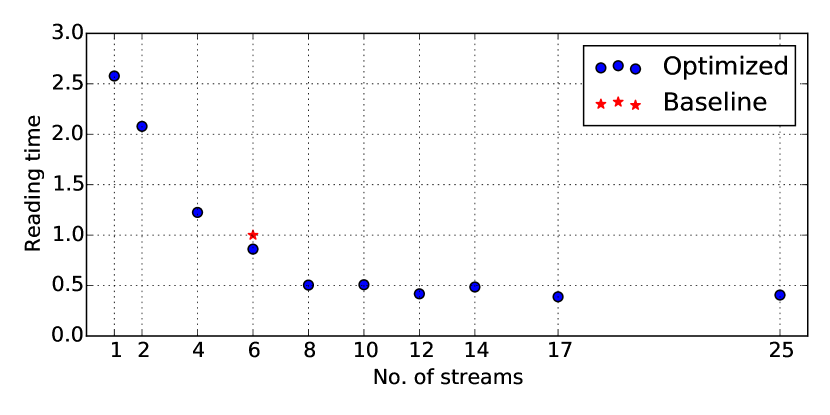
Figure 1: Evaluation of optimized streams. On the vertical axis $T_{\text{real}}$ is plotted with values normalized to the baseline, where the lines are grouped by physical similarity [10]. For the same number of streams, the disk reading time of the analysis jobs is improved by 15%, while adding two additional streams brings this to 50%.

5 Conclusion

We present a method for finding the optimal stream composition. It is flexible and can be used for different cost functions and numbers of streams. For the Tesla streams, it is possible to decrease the disk reading time of the analysis jobs by 15% while maintaining the line groupings and stream counts.

References

References

- [1] 2003 LHCb technical design report: Reoptimized detector design and performance
- [2] Aaij R et al. 2013 JINST 8 P04022 (Preprint 1211.3055)
- [3] Aaij R, Amato S, Anderlini L, Benson S, Cattaneo M, Clemencic M, Couturier B, Frank M, Gligorov V, Head T et al. 2016 Computer Physics Communications 208 35–42
- [4] Burke S, Campana S, Lanciotti E, Litmaath M, Lorenzo P, Miccio V, Nater C, Santinelli R and Sciabà A 2012 gLite 3.2 User Guide (CERN) URL https://edms.cern.ch/ui/file/722398/1.4/gLite-3-UserGuide.pdf
- [5] Brook N 2004 LHCb Computing Model Tech. Rep. LHCb-2004-119. CERN-LHCb-2004-119 CERN Geneva URL https://cds.cern.ch/record/811089
- [6] Paterson S K and Maier A 2008 Journal of Physics: Conference Series 119 072026 URL http://stacks.iop.org/1742-6596/119/i=7/a=072026
- [7] Pedregosa F, Varoquaux G, Gramfort A, Michel V, Thirion B, Grisel O, Blondel M, Prettenhofer P, Weiss R, Dubourg V et al. 2011 Journal of Machine Learning Research 12 2825–2830
- [8] Bishop C M 2006 Machine Learning 128 1–58
- [9] The Theano Development Team 2016 arXiv preprint arXiv:1605.02688
- [10] Benson S 2016 streams.py rev. 207995 URL https://svnweb.cern.ch/trac/lhcb/browser/DBASE/trunk/TurboStreamProd/python/TurboStreamProd/streams.py?rev=207995
- [11] LHCb Collaboration and others 2015 The DAVINCI project URL http://lhcb-release-area.web.cern.ch/LHCb-release-area/DOC/davinci