Origin of magnetic frustration in Bi₃Mn₄O₁₂(NO₃)

Abstract

Bi₃Mn₄O₁₂(NO₃) (BMNO) is a honeycomb bilayers anti-ferromagnet, not showing any ordering down to very low temperatures despite having a relatively large Curie-Weiss temperature. Using ab initio density functional theory, we extract an effective spin Hamiltonian for this compound. The proposed spin Hamiltonian consists of anti-ferrimagnetic Heisenberg terms with coupling constants ranging up to third intra-layer and fourth inter-layer neighbors. Performing Monte Carlo simulation, we obtain the temperature dependence of magnetic susceptibility and so the Curie-Weiss temperature and find the coupling constants which best matches with the experimental value. We discover that depending on the strength of the interlayer exchange couplings, two collinear spin configurations compete with each other in this system. Both states have in plane Néel character, however, at small interlayer coupling spin directions in the two layers are antiparallel (N₁ state) and discontinuously transform to parallel (N₂ state) by enlarging the interlayer couplings at a first order transition point. Classical Monte Carlo simulation and density matrix renormalization group calculations confirm that exchange couplings obtained for BMNO are in such a way that put this material at the phase boundary of a first order phase transition, where the trading between these two collinear spin states prevents it from setting in a magnetically ordered state.

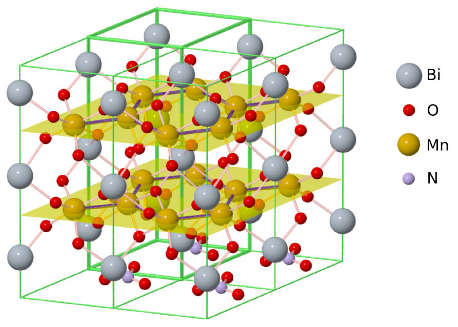
Bi₃Mn₄O₁₂(NO₃) (BMNO) is an experimental realization of frustrated honeycomb magnetic materials, synthesized by Smirnova et al. Smirnova et al. (2009). In this compound, the magnetic lattice can be effectively described by a weakly coupled honeycomb bilayers of Mn⁺⁴ ions (Fig. 1). The temperature dependence of magnetic susceptibility of BMNO does not indicate any ordering down to $T=0.4$K, in spite of the Curie-Weiss temperature $\theta_{\rm CW}\approx-257$K Smirnova et al. (2009); Onishi et al. (2012). The absence of long-range ordering in BMNO is also confirmed by specific heat measurements Smirnova et al. (2009); Onishi et al. (2012), neutron scattering Matsuda et al. (2010) and high-field electron spin relaxation (ESR) experiments Okubo et al. (2010). So far, the theoretical attempts to explain the magnetic properties of BMNO have been focusing on the frustration effect of second intra-layer coupling $J_{2}$ or the tendency toward dimerization by considering a large anti-ferromagnetic inter-layer nearest neighbor coupling $J_{1c}$  Kandpal and van den Brink (2011); Ganesh et al. (2011a, b); Oitmaa and Singh (2012); Okubo et al. (2012); Zhang et al. (2014); Albarracín and Rosales (2016); Bishop and Li (2016). In an attempt to calculate the exchange interactions by ab initio method, it is found that the dominant exchange interactions are nearest in-plane coupling ($J_{1}$) and also an effective inter-plane coupling ($J_{c}$) which exceeds $J_{1}$ Kandpal and van den Brink (2011). However, in that work the experimental positions of the atoms in the structure are taken without geometry optimization and only $5$ magnetic configurations are considered for the calculation of exchange interactions. In this paper, we obtain a Heisenberg spin Hamiltonian for BMNO, using an ab initio LDA+U calculation. In our calculations, we consider a detailed analysis of nonidentical Mn atoms which were assumed to be identical in the previous calculation Kandpal and van den Brink (2011). We show that how this consideration can affect the exchange couplings in the spin Hamiltonian. We find that in contrary to the previous works, none of $J_{2}$ and $J_{1c}$ are large enough to frustrate BMNO to reach an ordered state. Indeed, surprisingly the interlayer coupling constants are fined tuned in a way that make this system living at the edge boundary of two competing magnetic states.

Figure 1: (Color online) The $2\times 2$ supercell of BMNO. The thicker green lines show the primitive cell. Two (yellow transparent) planes show honeycomb lattices which are made of Mn atoms.

Figure 2: $J_{1}$, $J_{2}$ and $J_{3}$ indicate the Heisenberg exchange coupling constants between first, second and third nearest neighbor in-plane Mn⁺⁴ ions, respectively. $J_{1c}$, $J_{2c}$, $J_{3c}$ and $J_{4c}$ indicate the Heisenberg exchange coupling constants between inter-plane first, second and third nearest neighbor Mn⁺⁴ ions, respectively.

Ab initio method. To derive magnetic exchange couplings, we employ Density Functional Theory (DFT) with Full-Potential Local-Orbital minimum-basis (FPLO), using FPLO code Koepernik and Eschrig (1999) (FPLO14.00-45). For charge analysis we employ Projector Augmented Wave (PAW) method, using Quantum-Espresso (QE) distribution Giannozzi et al. (2009). To account for exchange-correlation interaction we use PBE functional Perdew et al. (1996) from Generalized Gradient Approximation (GGA). To improve estimation of electron-electron Coulomb interactions, we also add Hubbard-like $U$ correction to DFT calculations, i.e., DFT+$U$ Anisimov et al. (1991, 1993). To implement DFT+$U$, FPLO uses Liechtenstein’s approach Liechtenstein et al. (1995); Eschrig et al. (2003). In Liechtenstein’s approach the two parameters, $U$ (on-site Coulomb repulsion) and $J_{H}$ (the on-site Hund exchange) needs to be set, which we use $J_{H}=1.0$ eV and $U=1.5,2.0,3.0$ and $4.0$ eV.

Figure 3: (Color online) (top): The ab initio energy landscape (per Mn atom) of $54$ magnetic configurations obtained by DFT+$U$ with $U=1.5$ eV. The energies of magnetic configurations are respect to fully ferromagnetic state whose energy is set to $0$. (bottom): Three magnetic configurations N₁, N₂ and N₃.

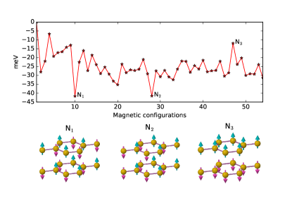
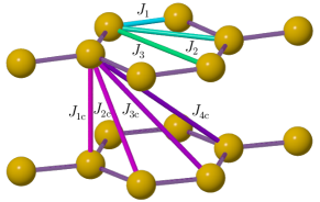
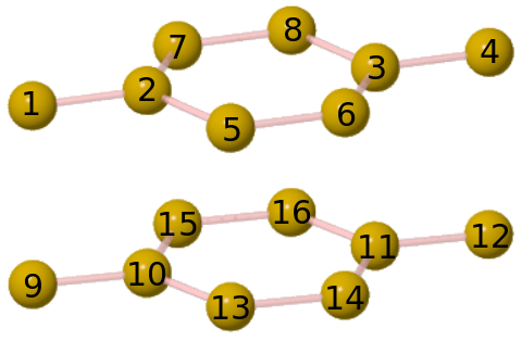
Spin Hamiltonian. The strategy of finding an effective spin Hamiltonian from ab initio calculations is to first compute the ground state energy for some given magnetic configurations. Then, mapping the energy difference of these configurations to an appropriate spin model gives us the coupling constants of the model. In this work, we use non-relativistic DFT, hence any magnetic anisotropy originating from the spin-orbit interaction is ignored in this approximation. Therefore, to leading order, we propose a spin Hamiltonian containing only bi-linear Heisenberg interactions, ${\cal H}_{\rm{Heisenberg}}=\sum_{i>j}J_{ij}\,{\bf n}_{i}\cdotp{\bf n}_{j}$, where ${\bf n}_{i}$ and ${\bf n}_{j}$ are classical unit vectors representing the orientation of the magnetic moments at sites $i$ and $j$, respectively, with exchange interactions $J_{ij}$ between them. The primitive cell of Bi₃Mn₄O₁₂(NO₃) contains $23$ atoms. Because of the limitation in computational resources, we use the $2\times 2$ supercell containing $92$ atoms (Fig. 1). This lets us calculate $J_{ij}$’s up to the third in-plane neighbor ($J_{1}$, $J_{2}$ and $J_{3}$) and up to the fourth inter-plane neighbor coupling ($J_{1c}$, $J_{2c}$, $J_{3c}$ and $J_{4c}$) (see figure 2). BMNO is metallic in GGA, however, implementing spin-polarized calculation makes this compound insulating, independent of its magnetic configuration. Within co-linear spin polarized GGA, the ground state is a Néel state in which the nearest neighbor Mn magnetic moments (in and out of plane) are anti-parallel with respect to each other. This magnetic configuration is marked by N₁ in Fig. 3. We calculated the total energy for more than $50$ independent magnetic configurations. Then employing the least square method, enables us to obtain the exchange couplings with the accuracy of $0.02$ meV. The top panel of figure 3 represents the energy landscape (per Mn atom) calculated for $54$ different magnetic configurations within the super-cell shown in Fig. 1. The detailed description of these configurations is given in Ref.sup . As it is obvious from this figure, the two configurations N₁ and N₂ (bottom panel of Fig. 3) are very close in energy space. In configuration N₂, the magnetic ordering in each honeycomb layer is Néel type, but unlike N₁, the magnetic moment orientations of two layer are parallel. The coupling constants of the Heisenberg Hamiltonian, obtained by different values of on-site Coulomb interaction $U$, are given in Table 1. We also checked that the exchange interactions between the adjacent honeycomb bilayers are negligible comparing to the ones inside the bilayers sup . It is important to mention that to achieve equal couplings between equivalent Mn ions in the two layers, we need to geometrically optimize the atomic positions rather than just using the experimental atomic positions (for the details see supplementary information sup ).

Table 1: Heisenberg constants obtained by ab initio calculations (LDA+$U$) using different $U$. The geometrically optimized structure (in the ferromagnetic state) is used in these calculations. The last column shows Curie-Weiss temperature obtained from Monte Carlo simulations for a system size with $N=4\times 24\times 24\times 1$. The experimental Curie-Weiss temperature is between $-257$K Smirnova et al. (2009) and $-222$K Onishi et al. (2012).

method	$U({\rm eV})$	$J_{1}\,({\rm meV})$	$J_{2}\,({\rm meV})$	$J_{3}\,({\rm meV})$	$J_{1c}\,({\rm meV})$	$J_{2c}\,({\rm meV})$	$J_{3c}\,({\rm meV})$	$J_{4c}\,({\rm meV})$	$\Theta_{CW}(K)$
FPLO	1.5	10.7	0.9	1.2	3.0	1.1	0.5	0.9	-244
	2.0	9.0	0.8	1.0	2.6	0.9	0.5	0.8	-203
	3.0	6.6	0.6	0.8	2.1	0.7	0.3	0.6	-144
	4.0	5.1	0.5	0.6	1.7	0.6	0.3	0.5	-111

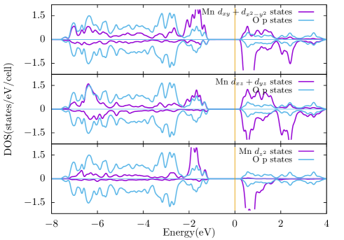
The Mn spin state. The bond valence sum indicates the valence state Bi${}^{3+}_{3}$Mn${}^{4+}_{4}$O${}^{2-}_{12}$(NO3)^- for BMNO Smirnova et al. (2009). However, using the charge analyzing code Critic2 de-la Roza et al. (2014, 2009), within GGA/PAW, we find the valence state Bi${}^{1.96+}_{3}$Mn${}^{1.87+}_{4}$O${}^{1.04-}_{12}$(NO3)^0.86- in N₁-configuration. This charge distribution will not change dramatically in the case of implementing DFT+$U$ even with large U parameter. We also made sure that using an all-electron method, such as FPLO, this picture of charge distribution remains nearly unchanged. The local density analysis (Lowdin charges), also proposes the charge distribution Bi${}^{1.49+}_{3}$Mn${}^{1.45+}_{4}$O${}^{0.74-}_{12}$(NO3)^0.40-. These charge analyses show that the Mn-O bonds are ionic-covalent instead of being completely ionic. Indeed, the reason for such a fractional charge distribution in BMNO is the strong hybridization between Mn d-orbitals and the neighboring O p-orbitals. This also lowers the magnetic moment of Mn ions from $3\mu_{B}$ to about $2.5\mu_{B}$ (see Table I in supplementary information sup ).

Figure 4: (Color online) Temperature dependence of the inverse normalized DC susceptibility ($1/\chi$) of BMNO obtained in experiment and MC simulations for different set of ab initio exchange couplings derived by using $U=1.5$ eV (filled circles), $U=2.0$ eV (triangles), $U=3.0$ eV (squares) and $U=4.0$ eV (pentagons). The experimental data (empty circles) is extracted from figure $7$ of Ref. Smirnova et al. (2009). For the normalization, all the data are divided by their values at $T=400$. The crossing of the line fitted at high temperatures to $1/\chi$ with the horizontal axis gives the Curie-Weiss temperature.

Figure 5: (Color online) Interlayer spin-spin correlation up to neighbor obtained by (top) MC simulation, (bottom DMRG (normalized by $S^{2}$). $J_{1},J_{2},J_{3},J_{1c},J_{3c}$ and $J_{4c}$ are kept fixed at those found by $U=1.5$ eV. The spin-spin correlations at $J_{2c}=1.100$ meV are obtained by using $U=1.5$ eV (blue circles) and compared with $J_{2c}=1.045$ (green diamonds) and $J_{2c}=1.155$ meV (red squares).

Figure 6: (Color online) Interlayer spin-spin correlation (normalized by $S^{2}$) up to fourth neighbor obtain by MC simulation . $J_{1},J_{2},J_{3},J_{2c},J_{3c}$ and $J_{4c}$ are kept fixed at the values obtained by $U=1.5$ eV. The spin-spin correlations at $J_{2c}=3.0$ meV are obtained by using $U=1.5$ eV (blue circles) and compared with $J_{1c}=3.15$ (red squares) and $J_{1c}=2.85$ meV (green diamonds).

Figure 7: (Color online) Interlayer spin-spin correlation (normalized by $S^{2}$) up to fourth neighbor obtain by MC simulation . $J_{1},J_{2},J_{3}$ are kept fixed at the values obtained using $U=1.5$ eV. The spin-spin correlations for the interlayer coupling calculated at $U=1.5$ (blue circles) are compared with the ones increased (red squares) and decreased (green diamonds) by 5 percent.

Figure 8: (Color online) DMRG results for the variation of spin-spin correlations for first, second, third in-plane neighbors and first inter-plane neighbors versus $J_{2c}/J_{1}$. Other coupling are fixed by those obtained by $U=1.5$ eV.

Figure 9: (Color online) DMRG results for the variation of the second interlayer spin-spin correlations versus $J_{2c}/J_{1}$, for lattices of size $4\times L^{2}$ with $L=2,3,4$. Other coupling are fixed by those obtained by $U=1.5$ eV.

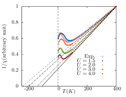
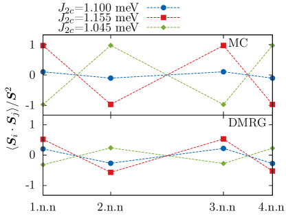
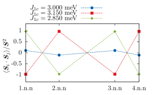
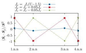
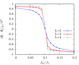
Monte Carlo Simulations. To gain insight into the finite temperature properties of the model Hamiltonian, we perform MC simulation. MC simulations are done on a $24\times 24\times 1$ supercell contains $2304$ Mn atoms with periodic boundary conditions. We use single spin Metropolis updating, $3\times 10^{6}$ MC steps for thermalization and $7\times 10^{6}$ MC samplings for the measurement of physical quantity. To reduce the correlations, we skip $5$ MC sweeps between successive data collections. In Figure 4 the temperature dependence of inverse magnetic susceptibility for the sets of exchange couplings obtained by ab initio method using $U=1.5,2.0,3.0,4.0$ eV and also the experimental values are compared. This figure shows a very good agreement between the experimental values and the set of exchanges obtained by using $U=1.5$ eV. The linear fit at high temperatures crosses the $T$-axis at a negative value which is the Curie-Weiss temperature $\theta_{CW}$. It can be seen that $\theta_{CW}$ increases by increasing the value of onsite Coulomb repulsion $U$. The $\theta_{CW}=-244K$ is closest to what has been measured experimentally. To speculate about the ground state of the Hamiltonian, we calculated the inter-layer spin-spin correlation at a low temperature, up to fourth neighbor (Fig. 5). The correlations are calculated by averaging over $5\times 10^{4}$ MC samplings at $T=2K$. As it can be seen from this figure, for the couplings corresponding to $U=1.5$ eV (Table I), the spin-spin correlations between the two layers are very small. We observe that, increasing (decreasing) the value of interlayer coupling by a little amount pushes the system toward N₁ (N₂) type ordering. Figure 5 shows the change of spin-spin correlation patterns, when $J_{2c}$ varies by only $\pm 5$ percent, while keeping the rest of the couplings unchanged. The same results are obtained when only $J_{1c}$ is changed while the other couplings are fixed (Fig.6) and also in the case that all the interlayer couplings are shifted up or downward (Fig.7). We also found that the small changes in the in-plane couplings do not induce spin ordering in the system.

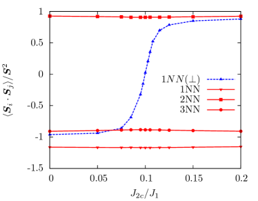
Quantum effects. To make an inquiry about the quantum correlations at zero temperature, we use the density matrix renormalization group (DMRG) technique based on a matrix product state representation to evaluate the spin correlations functions Dolfi et al. (2014). In our calculations, we adopt $S=3/2$ (which is the spin of Mn⁺⁴) and the lattices with $4\times L^{2}$ sites with $L=4$. The spin-spin correlations normalized by $S^{2}$ (shown in the bottom panel of Fig. 5), confirms the transition from N₁ to N₂ states at $J_{2c}/J_{1}\sim 0.1$, despite the weakening of the correlations as the effect of quantum fluctuations. This is while, the in-plane spins are in the Néel state, independent of the value of $J_{2c}$ (Fig. 8).

Now, we proceed to determine the order of N₁-N₂ transition for the set of exchange interactions obtained by using $U=1.5$ eV. Using Feynman-Hellmann theorem, the first derivative of the ground state energy with respect to a control parameter, say $J_{2c}$, is given by

$$\frac{\partial E_{0}}{\partial J_{2c}}=\langle\frac{\partial H}{\partial J_{2c}}\rangle=\frac{3}{2}N\langle{\mathbf{S}}_{i}\cdot{\mathbf{S}}_{j}\rangle_{2c},$$ (1)

in which $N=4L^{2}$ is the number of lattice points in a bilayer honeycomb of linear size $L$ and $\langle{\bf S}_{i}\cdot{\bf S}_{j}\rangle_{2c}$ denotes the spin-spin correlation between the second interlayer neighbors. Figure 9 represents the DMRG results for the variation of this correlation versus $J_{2c}/J_{1}$, for the lattices of linear sizes $L=2,3,4$. This figure shows a discontinuity in the second interlayer neighbor spin-spin correlation which becomes more pronounced by increasing the size of the system. Therefore equation 1 implies that the phase transition between these two ordered states is first order. Indeed, this result was expected because of different symmetries of N₁ and N₂ states.

Conclusion. In summary, we employed an ab initio LDA+U method to obtain the exchange coupling constants of a spin Hamiltonian for describing the magnetic properties of the honeycomb bilayer BMNO and figure out the reason that this compound does not show any ordering down to very low temperatures. Using $U=1.5$ eV, we found that a Hamiltonian containing only bilinear Heisenberg terms up to third in-plane and fourth out of plane neighbor, well matches the measured DC magnetic susceptibility for this material. Classical MC simulations and DMRG calculations on this spin Hamiltonian shows no sign of long-range ordering down to zero temperature. It is surprising that in BMNO the interlayer couplings are tuned in such a way to let this compound living at the phase boundary of the two collinear magnetic configurations N₁ and N₂. Indeed, the interlayer coupling $J_{1c}$ and $J_{3c}$ encourage the N₁ ordering, while $J_{2c}$ and $J_{4c}$ favor the N₂ state. Therefore, the balance between these two sets of couplings adjusts BMNO to be at the N₁-N₂ phase boundary. Hence, in the presence of any imbalance created as the effect of tension, compressive pressure, chemical doping, etc, the transition to N₁ or N₂ ordered states is expected. At this very special point, the spin-spin correlations in each layer are Néel type, however, there is almost a vanishing correlation between the two layers, making the dynamics of the two Néel states uncorrelated. The lack of correlations between the adjacent layer makes BMNO an effectively two-dimensional Heisenberg system for which there would be no finite temperature phase transition, according to the Mermin-Wagner theorem. It is also worthy to note that the presence of a strong enough spin-lattice interaction, could induce a spin-peierls lattice distortion and hence resolve the spin frustration. However, the reason that such a transition has not been observed experimentally, could be due to the small spin-orbit interaction in Mn atom which makes the temperature scale corresponding to the magneto-elastic interaction too small to cause an observable static lattice distortion in BMNO down to $50$ mK.

Supplemental Material

I charge analysis

In this section, we explain why Mn-O bonds has ionic-covalent character. In fact, the ionic-covalent character of Mn-O bonds can be obsereved in the hybridization of Mn-$d$ and O-$p$ orbitals. The point group of MnO₆ clusters in Bi₃Mn₄O₁₂(NO₃) is $C_{3}$, where the $C_{3}$-axis is perpendicular to honeycomb layer. Therefore, the Mn-$d$ orbitals are splitted as the effect of the crystal field into $d_{z^{2}}$, $(d_{xz},d_{yz})$ and $(d_{xy},d_{x^{2}-y^{2}})$. The projected density of states plotted in figure 10 together with the orbital occupation calculation shown in Table. 2, indicate that the hybridization among $d$ orbitals of Mn and $p$ orbitals of O makes the crystal field states $(d_{xz},d_{yz})$ and $(d_{xy},d_{x^{2}-y^{2}})$ to have fractional occupations.

Table 2: Charge distribution among Mn-$d$ orbitals obtained by GGA/PAW Lowdin charge analysis.

spin $d_{tot}$ $d_{z^{2}}$ $(d_{xz},d_{yz})$ $(d_{xy},d_{x^{2}-y^{2}})$ $\uparrow$ $3.8456$ $0.9825$ $0.6296$ $0.8020$ $\downarrow$ $1.2960$ $0.1890$ $0.2914$ $0.2621$

Therefore the bond valence sums (Bi${}^{3+}_{3}$Mn${}^{4+}_{4}$O${}^{2-}_{12}$(NO3)^-)  Smirnova et al. (2009) does not give rise to a true understanding of the charge distribution and also about magnetization of Mn atoms.

Figure 10 also shows a wide range of PDOS for all occupied $d$-orbitals, which could be a reason that why the onsite electron-electron repulsion parameter $U$ is not very large in this system.

Figure 10: Projected Density of States (PDOS) of Mn-$d$ and O-$p$ orbitals.

II Exchange constants

In the experimental structure of Bi₃Mn₄O₁₂(NO₃)  Smirnova et al. (2009) (with $P3$ space group), within the experimental error, vertical positions of Mn atoms in the unit cell are almost equal (Table 3). In the DFT calculations, we found that Mn₁ and Mn₂ as well as Mn₃ and Mn₄ do not have exactly the same vertical positions, even if exact site geometry optimization is performed. However, as Table 3 shows, in DFT, the vertical positions of Mn₁ and Mn₂ and also Mn₃ and Mn₄ are very close. The site geometry optimization has been done within $0.001$ eV/Ang accuracy. The space group of geometry optimization structure and experimental structure is the same (P3, No 143). So the space group of Bi3Mn4O14 doesn’t change during geometry optimization.

Table 3: Experiment and DFT Wycoff position of Mn atoms. The DFT calculation is done with $U=1.5$eV by FPLO method.

aotm Experiment Wycoff position DFT Wycoff position x y z x y z Mn₁ 2/3 1/3 0.855(5) 2/3 1/3 0.855500 Mn₂ 1/3 2/3 0.852(6) 1/3 2/3 0.855979 Mn₃ 2/3 1/3 0.218(5) 2/3 1/3 0.233593 Mn₄ 1/3 2/3 0.223(6) 1/3 2/3 0.233109

Since Mn atoms are not completely identical, we have to use more Heisenberg constants. For example, instead of only one $J_{1}$ for first nearest neighbor interaction we need to consider two: one between $\rm Mn_{1}$ and $\rm Mn_{2}$ ($J_{1}^{1,2})$ and the other between ${\rm Mn}_{3}$ and ${\rm Mn}_{4}$ ($J_{1}^{3,4}$). For the second neighbor couplings $J_{2}$ we also have $J_{2}^{1,1}$, $J_{2}^{2,2}$, $J_{2}^{3,3}$ and $J_{2}^{4,4}$. Similarly, there are variety of couplings for other inter and intra layer exchange interactions (see Table. 4).

To calculate the couplings of the Heisenberg Hamiltonian, we use $54$ magnetic configurations listed in Table. 6. Employing the least square method by considering these $54$ magnetic configurations, enables us to calculate the magnetic exchanges the within accuracy of 0.02 meV.

The ab initio results for the exchange couplings are given in Table. 4. These results are obtained after performing geometry optimization in a ferromagnetic configuration. The differences between the couplings of the same range are small ($\sim 0.1$meV), hence their arithmetic mean are reported in the main paper.

Using the experimental structure, the difference between the couplings of the same range are significant (see Table 5). For example, $J_{1}^{1,2}$=27.4 meV $J_{1}^{3,4}$=10.8 meV within GGA/FPLO method. So assuming identical Mn atoms for experimental structure to derive $J_{ij}$ are completely wrong.

In the main paper we assumed that the interaction between successive double layers could be ignored. To verify this assumption we calculate the energy difference of two magnetic configurations, a ferromagnetic configuration in which all the spins in all the bilayers are parallel and an anti-ferromagnetic configuration in which the spins in each bilayer are parallel, while they are antiparallel to the ones in neighboring bilayers. This energy difference gives an estimate of the strength of interaction between separated bilayers. Using FPLO method with $U=1.5$ eV, we obtain an energy difference (per Mn atom) of $\sim 0.3$ meV for these two configurations. This value is an order of magnitude less than the minimum energy difference (per Mn atom) of $54$ magnetic configurations inside each bilayer with respect to the ferromagnetic reference state, which is $6.6$ meV (Fig. 3 of main paper). Therefore it would be safe to neglect the bilayer-bilayer interaction.

Table 4: Heisenberg constants obtained by ab intio calculations (LDA+$U$) using FPLO. The structure, which is used in these calculations, is derived from geometry optimization of Bi₃Mn₄O₁₂(NO₃) in its feromagetic state.

method	$U$	$J_{1}^{1,2}$	$J_{1}^{3,4}$	$J_{2}^{1,1}$	$J_{2}^{2,2}$	$J_{2}^{3,3}$	$J_{2}^{4,4}$	$J_{3}^{(1,2)}$	$J_{3}^{3,4}$	$J_{1c}^{1,3}$	$J_{1c}^{2,4}$	$J_{2c}^{1,3}$	$J_{2c}^{2,4}$	$J_{3c}^{1,3}$	$J_{3c}^{2,4}$	$J_{4c}^{1,3}$	$J_{4c}^{2,4}$
FPLO	1.5	10.8	10.7	1.0	0.8	1.0	0.8	1.2	1.2	2.9	3.0	1.1	1.1	0.5	0.6	0.9	0.9
	2.0	9.0	9.0	0.9	0.7	0.9	0.7	1.0	1.0	2.6	2.6	1.0	0.9	0.4	0.5	0.8	0.8
	3.0	6.6	6.6	0.7	0.6	0.7	0.6	0.8	0.8	2.0	2.1	0.7	0.7	0.3	0.4	0.6	0.6
	4.0	5.1	5.1	0.5	0.4	0.5	0.5	0.6	0.7	1.6	1.7	0.6	0.6	0.3	0.3	0.5	0.5

Table 5: Heisenberg constants obtained by ab intio calculations (LDA+$U$) using different $U$ and different methods. The experimental structure is used in these calculations.

method	$U$	$J_{1}^{1,2}$	$J_{1}^{3,4}$	$J_{2}^{1,1}$	$J_{2}^{2,2}$	$J_{2}^{3,3}$	$J_{2}^{4,4}$	$J_{3}^{1,2}$	$J_{3}^{3,4}$	$J_{1c}^{1,3}$	$J_{1c}^{2,4}$	$J_{2c}^{1,3}$	$J_{2c}^{2,4}$	$J_{3c}^{1,3}$	$J_{3c}^{2,4}$	$J_{4c}^{1,3}$	$J_{4c}^{2,4}$
FPLO	0.0	27.4	10.8	0.9	0.7	2.5	2.0	1.2	2.2	4.6	5.9	1.8	1.3	0.2	0.6	1.0	0.7
	2.0	18.4	6.5	0.6	0.5	1.6	1.4	0.8	1.3	2.7	3.6	1.2	1.0	0.3	0.6	0.9	0.7
	3.0	14.1	4.3	0.5	0.4	1.2	1.1	0.6	1.0	2.2	2.8	0.9	0.8	0.3	0.4	0.7	0.5
	4.0	11.1	2.8	0.3	0.3	1.0	0.8	0.5	0.8	1.7	2.3	0.7	0.6	0.2	0.3	0.5	0.4

III Magnetic Configurations

In this section, we show the $54$ magnetic configurations used for the calculations of the Heisenberg coupling constants. To represent magnetic configurations, we assign a number on each Mn atoms in the $2\times 2\times 1$ supercell of Bi₃Mn₄O₁₂(NO₃) (figure 11), and then we specify the direction of Mn magnetic moments (up or down) by arrows shown in Table. 6.

Figure 11: Each Mn atoms are labeled by a number in $2\times 2\times 1$ supercell of Bi₃Mn₄O₁₂(NO₃)

Table 6: $54$ magnetic configurations which are used to derive $J_{ij}$.

Magnetic configuration	Mn1	Mn2	Mn3	Mn4	Mn5	Mn6	Mn7	Mn8	Mn9	Mn10	Mn11	Mn12	Mn13	Mn14	Mn15	Mn16
1	$\uparrow$	$\uparrow$	$\uparrow$	$\uparrow$	$\uparrow$	$\uparrow$	$\uparrow$	$\uparrow$	$\uparrow$	$\uparrow$	$\uparrow$	$\uparrow$	$\uparrow$	$\uparrow$	$\uparrow$	$\uparrow$
2	$\uparrow$	$\uparrow$	$\downarrow$	$\downarrow$	$\uparrow$	$\downarrow$	$\uparrow$	$\downarrow$	$\uparrow$	$\uparrow$	$\downarrow$	$\downarrow$	$\uparrow$	$\downarrow$	$\uparrow$	$\downarrow$
3	$\uparrow$	$\downarrow$	$\downarrow$	$\uparrow$	$\uparrow$	$\uparrow$	$\uparrow$	$\uparrow$	$\uparrow$	$\downarrow$	$\downarrow$	$\uparrow$	$\uparrow$	$\uparrow$	$\uparrow$	$\uparrow$
4	$\uparrow$	$\downarrow$	$\uparrow$	$\uparrow$	$\uparrow$	$\uparrow$	$\uparrow$	$\uparrow$	$\uparrow$	$\uparrow$	$\uparrow$	$\uparrow$	$\uparrow$	$\uparrow$	$\uparrow$	$\uparrow$
5	$\downarrow$	$\downarrow$	$\uparrow$	$\uparrow$	$\uparrow$	$\uparrow$	$\uparrow$	$\uparrow$	$\downarrow$	$\downarrow$	$\uparrow$	$\uparrow$	$\uparrow$	$\uparrow$	$\uparrow$	$\uparrow$
6	$\uparrow$	$\uparrow$	$\downarrow$	$\downarrow$	$\uparrow$	$\downarrow$	$\uparrow$	$\downarrow$	$\uparrow$	$\uparrow$	$\uparrow$	$\uparrow$	$\uparrow$	$\uparrow$	$\uparrow$	$\uparrow$
7	$\uparrow$	$\uparrow$	$\downarrow$	$\downarrow$	$\downarrow$	$\downarrow$	$\downarrow$	$\downarrow$	$\uparrow$	$\uparrow$	$\uparrow$	$\uparrow$	$\uparrow$	$\uparrow$	$\uparrow$	$\uparrow$
8	$\uparrow$	$\downarrow$	$\uparrow$	$\uparrow$	$\downarrow$	$\uparrow$	$\downarrow$	$\uparrow$	$\uparrow$	$\uparrow$	$\uparrow$	$\uparrow$	$\uparrow$	$\uparrow$	$\uparrow$	$\uparrow$
9	$\uparrow$	$\uparrow$	$\uparrow$	$\uparrow$	$\downarrow$	$\uparrow$	$\downarrow$	$\uparrow$	$\uparrow$	$\uparrow$	$\uparrow$	$\uparrow$	$\uparrow$	$\uparrow$	$\uparrow$	$\uparrow$
10(N1)	$\uparrow$	$\downarrow$	$\uparrow$	$\downarrow$	$\uparrow$	$\downarrow$	$\uparrow$	$\downarrow$	$\downarrow$	$\uparrow$	$\downarrow$	$\uparrow$	$\downarrow$	$\uparrow$	$\downarrow$	$\uparrow$
11	$\downarrow$	$\downarrow$	$\uparrow$	$\uparrow$	$\downarrow$	$\downarrow$	$\uparrow$	$\uparrow$	$\downarrow$	$\downarrow$	$\uparrow$	$\uparrow$	$\uparrow$	$\uparrow$	$\uparrow$	$\uparrow$
12	$\downarrow$	$\downarrow$	$\downarrow$	$\uparrow$	$\uparrow$	$\uparrow$	$\uparrow$	$\uparrow$	$\uparrow$	$\uparrow$	$\uparrow$	$\uparrow$	$\uparrow$	$\uparrow$	$\uparrow$	$\uparrow$
13	$\downarrow$	$\downarrow$	$\downarrow$	$\uparrow$	$\uparrow$	$\uparrow$	$\uparrow$	$\uparrow$	$\downarrow$	$\downarrow$	$\downarrow$	$\uparrow$	$\uparrow$	$\uparrow$	$\uparrow$	$\uparrow$
14	$\downarrow$	$\downarrow$	$\downarrow$	$\downarrow$	$\uparrow$	$\uparrow$	$\uparrow$	$\uparrow$	$\uparrow$	$\uparrow$	$\uparrow$	$\uparrow$	$\uparrow$	$\uparrow$	$\uparrow$	$\uparrow$
15	$\uparrow$	$\downarrow$	$\uparrow$	$\downarrow$	$\uparrow$	$\downarrow$	$\uparrow$	$\downarrow$	$\uparrow$	$\uparrow$	$\uparrow$	$\uparrow$	$\uparrow$	$\uparrow$	$\uparrow$	$\uparrow$
16	$\uparrow$	$\downarrow$	$\uparrow$	$\downarrow$	$\uparrow$	$\downarrow$	$\uparrow$	$\downarrow$	$\uparrow$	$\downarrow$	$\uparrow$	$\uparrow$	$\uparrow$	$\uparrow$	$\uparrow$	$\uparrow$
17	$\downarrow$	$\downarrow$	$\downarrow$	$\downarrow$	$\uparrow$	$\uparrow$	$\uparrow$	$\uparrow$	$\downarrow$	$\downarrow$	$\uparrow$	$\uparrow$	$\uparrow$	$\uparrow$	$\uparrow$	$\uparrow$
18	$\downarrow$	$\downarrow$	$\downarrow$	$\downarrow$	$\uparrow$	$\uparrow$	$\uparrow$	$\uparrow$	$\downarrow$	$\downarrow$	$\downarrow$	$\downarrow$	$\uparrow$	$\uparrow$	$\uparrow$	$\uparrow$
19	$\uparrow$	$\downarrow$	$\uparrow$	$\downarrow$	$\uparrow$	$\downarrow$	$\uparrow$	$\downarrow$	$\uparrow$	$\downarrow$	$\downarrow$	$\uparrow$	$\uparrow$	$\uparrow$	$\uparrow$	$\uparrow$
20	$\uparrow$	$\downarrow$	$\uparrow$	$\downarrow$	$\uparrow$	$\downarrow$	$\uparrow$	$\downarrow$	$\uparrow$	$\downarrow$	$\downarrow$	$\downarrow$	$\uparrow$	$\uparrow$	$\uparrow$	$\uparrow$
21	$\uparrow$	$\downarrow$	$\uparrow$	$\uparrow$	$\downarrow$	$\uparrow$	$\uparrow$	$\downarrow$	$\uparrow$	$\downarrow$	$\uparrow$	$\uparrow$	$\downarrow$	$\uparrow$	$\uparrow$	$\uparrow$
22	$\downarrow$	$\downarrow$	$\downarrow$	$\downarrow$	$\uparrow$	$\uparrow$	$\uparrow$	$\uparrow$	$\uparrow$	$\uparrow$	$\downarrow$	$\uparrow$	$\downarrow$	$\uparrow$	$\uparrow$	$\uparrow$
23	$\uparrow$	$\uparrow$	$\downarrow$	$\downarrow$	$\uparrow$	$\uparrow$	$\downarrow$	$\uparrow$	$\downarrow$	$\uparrow$	$\uparrow$	$\downarrow$	$\uparrow$	$\uparrow$	$\uparrow$	$\downarrow$
24	$\uparrow$	$\uparrow$	$\downarrow$	$\uparrow$	$\uparrow$	$\uparrow$	$\downarrow$	$\uparrow$	$\downarrow$	$\uparrow$	$\uparrow$	$\downarrow$	$\uparrow$	$\uparrow$	$\uparrow$	$\downarrow$
25	$\downarrow$	$\uparrow$	$\downarrow$	$\downarrow$	$\downarrow$	$\downarrow$	$\downarrow$	$\downarrow$	$\downarrow$	$\uparrow$	$\downarrow$	$\uparrow$	$\uparrow$	$\uparrow$	$\downarrow$	$\uparrow$
26	$\uparrow$	$\uparrow$	$\downarrow$	$\uparrow$	$\uparrow$	$\downarrow$	$\downarrow$	$\uparrow$	$\uparrow$	$\uparrow$	$\uparrow$	$\uparrow$	$\uparrow$	$\uparrow$	$\downarrow$	$\uparrow$
27	$\uparrow$	$\uparrow$	$\downarrow$	$\downarrow$	$\uparrow$	$\downarrow$	$\downarrow$	$\uparrow$	$\uparrow$	$\uparrow$	$\downarrow$	$\uparrow$	$\downarrow$	$\uparrow$	$\uparrow$	$\downarrow$
28(N2)	$\uparrow$	$\downarrow$	$\uparrow$	$\downarrow$	$\uparrow$	$\downarrow$	$\uparrow$	$\downarrow$	$\uparrow$	$\downarrow$	$\uparrow$	$\downarrow$	$\uparrow$	$\downarrow$	$\uparrow$	$\downarrow$
29	$\downarrow$	$\downarrow$	$\downarrow$	$\downarrow$	$\uparrow$	$\downarrow$	$\uparrow$	$\downarrow$	$\uparrow$	$\uparrow$	$\downarrow$	$\uparrow$	$\downarrow$	$\uparrow$	$\uparrow$	$\uparrow$
30	$\downarrow$	$\downarrow$	$\downarrow$	$\uparrow$	$\downarrow$	$\uparrow$	$\downarrow$	$\uparrow$	$\downarrow$	$\downarrow$	$\uparrow$	$\downarrow$	$\downarrow$	$\uparrow$	$\uparrow$	$\uparrow$
31	$\downarrow$	$\uparrow$	$\downarrow$	$\uparrow$	$\uparrow$	$\uparrow$	$\uparrow$	$\uparrow$	$\uparrow$	$\downarrow$	$\uparrow$	$\uparrow$	$\downarrow$	$\downarrow$	$\downarrow$	$\uparrow$
32	$\uparrow$	$\uparrow$	$\uparrow$	$\uparrow$	$\downarrow$	$\downarrow$	$\downarrow$	$\uparrow$	$\uparrow$	$\uparrow$	$\downarrow$	$\uparrow$	$\downarrow$	$\uparrow$	$\downarrow$	$\uparrow$
33	$\uparrow$	$\uparrow$	$\uparrow$	$\downarrow$	$\uparrow$	$\downarrow$	$\downarrow$	$\downarrow$	$\downarrow$	$\uparrow$	$\downarrow$	$\downarrow$	$\downarrow$	$\uparrow$	$\uparrow$	$\uparrow$
34	$\downarrow$	$\downarrow$	$\uparrow$	$\downarrow$	$\uparrow$	$\uparrow$	$\downarrow$	$\downarrow$	$\downarrow$	$\downarrow$	$\downarrow$	$\uparrow$	$\uparrow$	$\downarrow$	$\uparrow$	$\uparrow$
35	$\downarrow$	$\uparrow$	$\downarrow$	$\downarrow$	$\downarrow$	$\uparrow$	$\downarrow$	$\downarrow$	$\downarrow$	$\downarrow$	$\uparrow$	$\uparrow$	$\downarrow$	$\downarrow$	$\downarrow$	$\downarrow$
36	$\downarrow$	$\uparrow$	$\downarrow$	$\downarrow$	$\uparrow$	$\uparrow$	$\downarrow$	$\downarrow$	$\uparrow$	$\uparrow$	$\uparrow$	$\uparrow$	$\uparrow$	$\uparrow$	$\downarrow$	$\uparrow$
37	$\downarrow$	$\downarrow$	$\uparrow$	$\uparrow$	$\downarrow$	$\downarrow$	$\uparrow$	$\downarrow$	$\downarrow$	$\uparrow$	$\uparrow$	$\uparrow$	$\downarrow$	$\uparrow$	$\downarrow$	$\downarrow$
38	$\uparrow$	$\uparrow$	$\uparrow$	$\downarrow$	$\uparrow$	$\uparrow$	$\uparrow$	$\downarrow$	$\uparrow$	$\uparrow$	$\downarrow$	$\downarrow$	$\downarrow$	$\uparrow$	$\uparrow$	$\uparrow$
39	$\uparrow$	$\downarrow$	$\downarrow$	$\uparrow$	$\downarrow$	$\downarrow$	$\uparrow$	$\downarrow$	$\downarrow$	$\downarrow$	$\downarrow$	$\uparrow$	$\uparrow$	$\uparrow$	$\downarrow$	$\downarrow$
40	$\uparrow$	$\downarrow$	$\uparrow$	$\uparrow$	$\uparrow$	$\uparrow$	$\uparrow$	$\uparrow$	$\uparrow$	$\downarrow$	$\downarrow$	$\downarrow$	$\downarrow$	$\uparrow$	$\uparrow$	$\uparrow$
41	$\downarrow$	$\uparrow$	$\uparrow$	$\uparrow$	$\uparrow$	$\downarrow$	$\downarrow$	$\downarrow$	$\uparrow$	$\downarrow$	$\uparrow$	$\downarrow$	$\downarrow$	$\downarrow$	$\uparrow$	$\uparrow$
42	$\uparrow$	$\uparrow$	$\uparrow$	$\downarrow$	$\downarrow$	$\downarrow$	$\downarrow$	$\downarrow$	$\uparrow$	$\uparrow$	$\uparrow$	$\uparrow$	$\uparrow$	$\downarrow$	$\uparrow$	$\downarrow$
43	$\uparrow$	$\uparrow$	$\downarrow$	$\downarrow$	$\downarrow$	$\downarrow$	$\downarrow$	$\uparrow$	$\downarrow$	$\downarrow$	$\downarrow$	$\downarrow$	$\downarrow$	$\uparrow$	$\uparrow$	$\uparrow$
44	$\downarrow$	$\uparrow$	$\uparrow$	$\uparrow$	$\uparrow$	$\uparrow$	$\uparrow$	$\uparrow$	$\downarrow$	$\downarrow$	$\downarrow$	$\uparrow$	$\uparrow$	$\uparrow$	$\uparrow$	$\downarrow$
45	$\downarrow$	$\uparrow$	$\uparrow$	$\downarrow$	$\downarrow$	$\uparrow$	$\downarrow$	$\downarrow$	$\downarrow$	$\downarrow$	$\downarrow$	$\downarrow$	$\uparrow$	$\uparrow$	$\uparrow$	$\uparrow$
46	$\uparrow$	$\uparrow$	$\downarrow$	$\downarrow$	$\downarrow$	$\uparrow$	$\downarrow$	$\uparrow$	$\uparrow$	$\uparrow$	$\uparrow$	$\downarrow$	$\uparrow$	$\downarrow$	$\downarrow$	$\uparrow$
47(N${}_{3})$	$\uparrow$	$\uparrow$	$\uparrow$	$\uparrow$	$\uparrow$	$\uparrow$	$\uparrow$	$\uparrow$	$\downarrow$	$\downarrow$	$\downarrow$	$\downarrow$	$\downarrow$	$\downarrow$	$\downarrow$	$\downarrow$
48	$\downarrow$	$\downarrow$	$\downarrow$	$\downarrow$	$\downarrow$	$\downarrow$	$\downarrow$	$\uparrow$	$\uparrow$	$\uparrow$	$\uparrow$	$\uparrow$	$\downarrow$	$\downarrow$	$\downarrow$	$\uparrow$
49	$\uparrow$	$\downarrow$	$\downarrow$	$\downarrow$	$\downarrow$	$\uparrow$	$\downarrow$	$\downarrow$	$\downarrow$	$\downarrow$	$\uparrow$	$\downarrow$	$\downarrow$	$\downarrow$	$\downarrow$	$\uparrow$
50	$\downarrow$	$\downarrow$	$\uparrow$	$\downarrow$	$\uparrow$	$\uparrow$	$\uparrow$	$\downarrow$	$\downarrow$	$\downarrow$	$\downarrow$	$\uparrow$	$\downarrow$	$\uparrow$	$\uparrow$	$\downarrow$
51	$\uparrow$	$\uparrow$	$\downarrow$	$\uparrow$	$\uparrow$	$\downarrow$	$\uparrow$	$\downarrow$	$\downarrow$	$\uparrow$	$\uparrow$	$\downarrow$	$\downarrow$	$\uparrow$	$\downarrow$	$\uparrow$
52	$\downarrow$	$\uparrow$	$\downarrow$	$\downarrow$	$\downarrow$	$\downarrow$	$\downarrow$	$\uparrow$	$\downarrow$	$\uparrow$	$\downarrow$	$\uparrow$	$\downarrow$	$\uparrow$	$\downarrow$	$\downarrow$
53	$\uparrow$	$\uparrow$	$\downarrow$	$\uparrow$	$\uparrow$	$\downarrow$	$\uparrow$	$\uparrow$	$\downarrow$	$\downarrow$	$\uparrow$	$\uparrow$	$\downarrow$	$\downarrow$	$\downarrow$	$\uparrow$
54	$\downarrow$	$\uparrow$	$\downarrow$	$\uparrow$	$\downarrow$	$\uparrow$	$\uparrow$	$\uparrow$	$\downarrow$	$\downarrow$	$\uparrow$	$\uparrow$	$\downarrow$	$\uparrow$	$\downarrow$	$\uparrow$

IV DMRG results analysis

We use density matrix renormalization group (DMRG) techniques based on a matrix product state (MPS) representation to evaluate the spin correlation functions. MPS is an variational ansatz that the variational parameters can be controlled by the matrix size, M, called the bond dimension. The ground state converges after sweeping a few times through the system.

We carry out 10 sweeps to converge the ground state within an error less than $3$ percent near the phase transition point. Moreover, we compare the correlation functions calculated using different bond dimension and find that the error of the results is less than $1.3$ percent. Away from the phase transition point, the errors are less than these values and reach to $0.4$ percent.

References

- Smirnova et al. (2009) O. Smirnova, M. Azuma, N. Kumada, Y. Kusano, M. Matsuda, Y. Shimakawa, T. Takei, Y. Yonesaki, and N. Kinomura, Journal of the American Chemical Society 131, 8313 (2009).
- Onishi et al. (2012) N. Onishi, K. Oka, M. Azuma, Y. Shimakawa, Y. Motome, T. Taniguchi, M. Hiraishi, M. Miyazaki, T. Masuda, A. Koda, et al., Physical Review B 85, 184412 (2012).
- Matsuda et al. (2010) M. Matsuda, M. Azuma, M. Tokunaga, Y. Shimakawa, and N. Kumada, Phys. Rev. Lett. 105, 187201 (2010).
- Okubo et al. (2010) S. Okubo, F. Elmasry, W. Zhang, M. Fujisawa, T. Sakurai, H. Ohta, M. Azuma, O. A. Sumirnova, and N. Kumada, Journal of Physics: Conference Series 200, 022042 (2010).
- Kandpal and van den Brink (2011) H. C. Kandpal and J. van den Brink, Physical Review B 83, 140412 (2011).
- Ganesh et al. (2011a) R. Ganesh, D. Sheng, Y.-J. Kim, and A. Paramekanti, Physical Review B 83, 144414 (2011a).
- Ganesh et al. (2011b) R. Ganesh, S. V. Isakov, and A. Paramekanti, Physical Review B 84, 214412 (2011b).
- Oitmaa and Singh (2012) J. Oitmaa and R. Singh, Physical Review B 85, 014428 (2012).
- Okubo et al. (2012) S. Okubo, T. Ueda, H. Ohta, W. Zhang, T. Sakurai, N. Onishi, M. Azuma, Y. Shimakawa, H. Nakano, and T. Sakai, Phys. Rev. B 86, 140401 (2012).
- Zhang et al. (2014) H. Zhang, M. Arlego, and C. Lamas, Physical Review B 89, 024403 (2014).
- Albarracín and Rosales (2016) F. G. Albarracín and H. Rosales, Physical Review B 93, 144413 (2016).
- Bishop and Li (2016) R. Bishop and P. Li, arXiv preprint arXiv:1611.03287 (2016).
- Koepernik and Eschrig (1999) K. Koepernik and H. Eschrig, Phys. Rev. B 59, 1743 (1999).
- Giannozzi et al. (2009) P. Giannozzi et al., Journal of Physics: Condensed Matter 21, 395502 (2009).
- Perdew et al. (1996) J. P. Perdew, K. Burke, and M. Ernzerhof, Phys. Rev. Lett. 77, 3865 (1996).
- Anisimov et al. (1991) V. I. Anisimov, J. Zaanen, and O. K. Andersen, Phys. Rev. B 44, 943 (1991).
- Anisimov et al. (1993) V. I. Anisimov, I. V. Solovyev, M. A. Korotin, M. T. Czyżyk, and G. A. Sawatzky, Phys. Rev. B 48, 16929 (1993).
- Liechtenstein et al. (1995) A. I. Liechtenstein, V. I. Anisimov, and J. Zaanen, Phys. Rev. B 52, R5467 (1995).
- Eschrig et al. (2003) H. Eschrig, K. Koepernik, and I. Chaplygin, Journal of Solid State Chemistry 176, 482 (2003), special issue on The Impact of Theoretical Methods on Solid-State Chemistry.
- (20) See Supplementary Material at [URL].
- de-la Roza et al. (2014) A. O. de-la Roza, E. R. Johnson, and V. Luaña, Computer Physics Communications 185, 1007 (2014).
- de-la Roza et al. (2009) A. O. de-la Roza, M. Blanco, A. M. Pendás, and V. Luaña, Computer Physics Communications 180, 157 (2009).
- Dolfi et al. (2014) M. Dolfi, B. Bauer, S. Keller, A. Kosenkov, T. Ewart, A. Kantian, T. Giamarchi, and M. Troyer, Computer Physics Communications 185, 3430 (2014).