Learning Normalized Inputs for Iterative Estimation in Medical Image Segmentation

Abstract

In this paper, we introduce a simple, yet powerful pipeline for medical image segmentation that combines Fully Convolutional Networks (FCNs) with Fully Convolutional Residual Networks (FC-ResNets). We propose and examine a design that takes particular advantage of recent advances in the understanding of both Convolutional Neural Networks as well as ResNets. Our approach focuses upon the importance of a trainable pre-processing when using FC-ResNets and we show that a low-capacity FCN model can serve as a pre-processor to normalize medical input data. In our image segmentation pipeline, we use FCNs to obtain normalized images, which are then iteratively refined by means of a FC-ResNet to generate a segmentation prediction. As in other fully convolutional approaches, our pipeline can be used off-the-shelf on different image modalities. We show that using this pipeline, we exhibit state-of-the-art performance on the challenging Electron Microscopy benchmark, when compared to other 2D methods. We improve segmentation results on CT images of liver lesions, when contrasting with standard FCN methods. Moreover, when applying our 2D pipeline on a challenging 3D MRI prostate segmentation challenge we reach results that are competitive even when compared to 3D methods. The obtained results illustrate the strong potential and versatility of the pipeline by achieving highly accurate results on multi-modality images from different anatomical regions and organs.

I Introduction

Segmentation is an active area of research in medical image analysis. With the introduction of Convolutional Neural Networks (CNNs), significant improvements in performance have been achieved in many standard datasets. For example, for the EM ISBI 2012 dataset [5], PROMISE12 challenge or MS lesions [42], the top entries are built on CNNs [38, 13, 21, 50].

The common view on CNN models is based on a representation learning perspective [20, 19]. This view assumes that a CNN is built from layers (convolutional operations and non-linearities) that learn increasing levels of abstraction. In [51], these different levels of abstraction were visualized, showing that in the first layer the network learns simple edge and blob detectors (e.g. Gabor-like filters), the second layer learns combination of these simple features, while the deeper layers learn to represent more complex object contours, such as faces or flowers. Moreover, in [47], it was shown that removing any single layer of the network after training/finetuning can significantly harm the network’s performance, implying that the transformations learnt by a CNN layer are very different from an identity mapping.

Recently, a new class of models called Residual Networks (ResNets) have been introduced [23, 24]. ResNets are built from hundreds of residual blocks. Each residual block is composed of two paths: the first one applies a series of nonlinear transformations (typically two or three transformations composed of Batch Normalization [43], convolution and a ReLu non-linearity), while the second one is an identity mapping. These two paths are summed up at the end of a residual block. This small architectural modification has three important implications. First, the gradient can flow uninterrupted allowing parameters to be updated even in very deep networks. Second, ResNets are robust to layer removal at training time [25] and at inference time [47] implying that the operations applied by a single layer are only a small modification to identity operation. Third, ResNets are robust to layers permutation [47], suggesting that neighboring layers perform similar operations. These characteristics are not shared with traditional CNNs and researchers have attempted to propose possible explanations on the internal behaviors and mechanisms with ResNet-like models. Recently, two possible explanations of ResNets-like models have emerged. The first, explains the behavior of ResNets in terms of an embedding of relatively shallow networks [47]. The second, suggests that ResNets perform iterative estimation, where the input to the model is iteratively modified by small transformations [20, 30].

In recent years, state of the art segmentation methods for medical images have been based on Fully Convolutional Networks (FCNs) [32, 38]. While CNNs typically consist of a contracting path composed of convolutional, pooling and fully connected layers, FCNs add an expanding path composed of transposed convolutions or unpooling layers. The expanding path recovers spatial information by merging features skipped from the various resolution levels on the contracting path. Variants of these skip connections are proposed in the literature. In [32], upsampled feature maps are summed with feature maps skipped from the contractive path, while [38] concatenate them and add convolutions and non-linearities between each upsampling step. These skip connections have been shown to help recover the full spatial resolution at the network’s output, making fully convolutional methods suitable for semantic segmentation. Since traditional FCNs are an extension of CNNs, they can be explained by the representation learning perspective on deep learning.

Although deep learning methods have proved their potential in medical image segmentation, their performance strongly depends on the quality of pre-processing and post-processing steps [22]. Thus, traditional image segmentation pipelines based on FCNs are often complemented by pre-processing and post-processing blocks (see Figure1(a)). Pre-processing methods vary among different imaging modalities and can include operations like standardization, histogram equalization, value clipping or range normalization (e.g. dividing by maximum intensity value). The tools of choice for post-processing are either based on Conditional Random Fields [28] to account for spatial consistency of the output prediction or on morphological operations to clean the output prediction.

In [17], the Fully Convolutional Residual Networks (FC-ResNets) are introduced. FC-ResNets incorporate additional shortcut paths and, thus, increase the number of connections within a segmentation network. These additional shortcut paths have been shown not only to improve the segmentation accuracy but also help the network optimization process, resulting in faster convergence of the training. Since FC-ResNets are an extension of ResNets, their behavior should be interpreted in terms of iterative estimation or embedding of relatively shallow networks. Moreover, not surprisingly, these FC-ResNets are more susceptible to image pre-processing than FCNs, their performance is highly dependent on proper data preparation (e.g. data standardization or range normalization).

(a) Traditional pipeline

(b) Our pipeline

Figure 1: Traditional pipeline for medical image segmentation (a) and proposed pipeline for medical image segmentation (b).

In this paper, we take advantage of recent advances in the understanding of both CNNs as well as ResNets and propose a new medical image segmentation pipeline. We use a FCN to obtain pre-normalized images, which are then iteratively refined by means of a FC-ResNet to generate a segmentation prediction (see Figure 1(b)).

Thus, in our pipeline, the FCN can be thought of as a pre-processor that is learnt by means of back-propagation, and FC-ResNet can be thought as a powerful classifier that is an ensemble of exponential number of shallow models. This small modification to current segmentation pipelines allows to remove hand-crafted data pre-processing and to build end-to-end systems trained with back-propagation that achieve surprisingly good performance in segmentation tasks for bio-medical images. Our pipeline reaches state-of-the art for 2D methods on electron microscopy (EM) ISBI benchmark dataset [5] and outperforms both standard FCN [32, 38] and FC-ResNet [17] on in-house CT liver lesion segmentation dataset. Moreover, while applying our 2D pipeline off-the-shelf on a challenging 3D MRI prostate segmentation challenge, we reach results that are competitive even when compared to 3D methods.

Thus, the contributions in this paper can be summarized as follows:

• We combine Fully Convolutional Residual Networks with Fully Convolutional Networks (Section III).

• We show that a very deep network without any hand-designed pre- or post-processing achieves state-of-the-art performance on the challenging EM ISBI benchmark [5] (Section IV-A).

• We show that our pipeline outperforms other common FCN-based segmentation pipelines on our in-house CT liver lesion dataset (Section IV-B).

• We show that our 2D pipeline can be applied to untreated MR images reaching competitive results on challenging 3D MRI prostate segmentation task, outperforming many 3D based approaches (Section IV-C).

• We show that a FCN based pre-processor normalizes the data to the values adequate for FC-ResNet (Section IV-D).

II Background

Recent advances in medical image segmentation often involve convolutional networks. Most of these state-of-the-art approaches are based on either variants of FCNs (FCN8 or UNet) or CNN architectures. FCN architectures process the input image end-to-end and provide a full resolution segmentation map, whereas CNN variants are applied to input patches and aim to solely classify the central pixel of each patch. In many cases, the application of an FCN/CNN is preceded by a pre-processing step and followed by a post-processing step. The former aims to account for the variability in the input images, whereas the latter helps refine the predictions made by the FCN/CNN.

In the remainder of this section, we review segmentation pipelines in medical imaging based on deep neural networks, for different imaging modalities and organs, with a particular focus on pre-processing and post-processing steps proposed to normalize and regularize data, respectively.

Electron Microscopy (EM). EM is widely used to study synapses and other sub-cellular structures in the mammalian nervous system. EM data is the basis of two medical imaging segmentation challenges: 2D [5] and 3D [2]. The core of the best performing methods is based on a patch-based CNN [16], FCN8 [13], UNet [38] and FC-ResNets [17, 37, 18]. The methods account for gray scale value variability by employing data augmentation (e.g. intensity shifts [38, 37]) or data pre-processing (e.g standardization [17] or rescaling [37]). As for post-processing, a variety of FCN prediction refinement techniques have been proposed. In [6], a minimum cost multi-cut approach is introduced, in [18, 13], watershed algorithm is used, while in [37], median filtering is employed to improve EM segmentation results.

(a) FC-ResNet

(b) Bottleneck block

(c) Simple block

Figure 2: An example of residual network for image segmentation. (a) Residual Network with long skip connections built from bottleneck blocks, (b) bottleneck block and (c) simple block. Blue color indicates the blocks where a downsampling is optionally performed, yellow color depicts the (optional) upsampling blocks, dashed arrow in figures (b) and (c) indicates possible long skip connections. Note that blocks (b) and (c) can have a dropout [40] layer (depicted with dashed line rectangle). The downsampling operation is performed with strided convolution in the bottleneck block and with maxpooling in the simple block.

Magnetic Resonance Imaging (MRI). MRI is used for detection, classification of lesions and tumor staging. As in many medical imaging applications, deep learning methods are nowadays playing an important role in the segmentation of lesions and organs from MRI scans, consistently improving state-of-the-art performance. Patch-based CNN architectures have been used to segment brain tumors [27, 36] and MS lesions [8]. Variants of FCN8 and UNets have also been applied to segment brain tumors [11, 33, 34, 9, 52], whereas FC-ResNets have been successfully employed to segment white and gray matter in the brain [12] and prostate [50, 35]. To account for 3D information, some of the proposed architectures apply convolutions in a 3D fashion [12, 9, 36, 27, 35] or make use of recurrent neural networks (LSTMs or GRUs) [4, 41]. As in the previous modalities, pre-processing techniques are applied to the input of the network. MRI pre-processing techniques include intensity normalization [8, 12], rescaling [11], standardization [27, 36, 9, 52, 12, 4, 41, 50], N4 bias correction [36, 52, 8, 41] and histogram equalization [11]. Again, post-processing involving morphological operations [36, 52], conditional random fiels (CRFs) [27, 52] and interpolation [4] are often used to refine segmentation maps.

Computed Tomography (CT). Finally, CT scans are widely used by clinicians to detect a large variety of lesions in different organs. Patch-based CNNs have been used in the literature to segment pathological kidneys [53, 44], liver tumors [48], pancreas [39] and urinary bladder [10]. FCN8 and UNet variants have also been tried on CT scans, e.g. to segment liver tumors [7, 15]. In many cases, CT scans are pre-processed by standardizing [44, 29, 10], clipping [15], applying Gaussian smoothing [29, 10] or histogram equalization [15] to the input. Gaussian noise injection has also been explored as part of data augmentation to account for noise level variability in the CT scans [15]. As in the other modalities, the most frequently used post-processing methods include morphological operations [44, 48, 39], CRFs [15] and level sets [10] to refine the segmentation proposals.

III Method

In this section we explain our segmentation pipeline. As explained in Section I, our approach combines a FCN model with a FC-ResNet model (see Figure 1(b)). The goal of FCN in our pipeline is to pre-process the image to a format that can be iteratively refined by FC-ResNet. In the remainder of this section, we describe the architecture of our FCN-based pre-processor (see Subsection III-A), our FC-ResNet (see Subsection III-B) as well as the loss function used to train our pipeline (see Subsection III-C).

III-A Fully Convolutional pre-processor

Our FCN takes as input a raw image of size $N\times N\times 1$ (e.g. CT scan slice or EM image) without applying any pre-processing and outputs a processed $N\times N\times 1$ feature map. The FCN pre-processor architecture is described as a variation of the UNet model from [38] (see Table I for details). The contracting path is built by alternating convolutions and max pooling operations, whereas the expanding path is built by alternating convolutions and repeat operations. The expanding path recovers spatial information, lost in pooling operations, by concatenating the corresponding feature maps from the contracting path. In total, the model has 4 pooling operations and 4 repeat operations. All $3\times 3$ convolutions are followed by ReLU non-linearity, while no non-linearity follows the $1\times 1$ and $2\times 2$ convolutions. In our experiments, we reduce the number of feature maps by a factor of 4 when compared to the original UNet (e. g. our first layer has 16 feature maps instead of 64 as in the original model). This step significantly reduces the memory foot-print of the FCN-based pre-processor. Thus, our UNet-like pre-processor has $1.8$ million trainable parameters (vs 33 million in the original implementation of [38]). Note that the UNet could potentially be replaced by other FCN models (e.g. FCN8 [32]).

III-B Iterative Estimation with FC-ResNets

ResNets [23] introduce a residual block that sums the identity mapping of the input to the output of a layer allowing for the reuse of features and permitting the gradient to flow directly to earlier layers. The resulting output $x_{\ell}$ of the $\ell^{th}$ block becomes

$$x_{\ell}=H_{\ell}(x_{\ell-1})+x_{\ell-1},$$ (1)

where $H$ is defined as the repetition (2 or 3 times) of a block composed of Batch Normalization (BN) [26] followed by ReLU and a convolution.

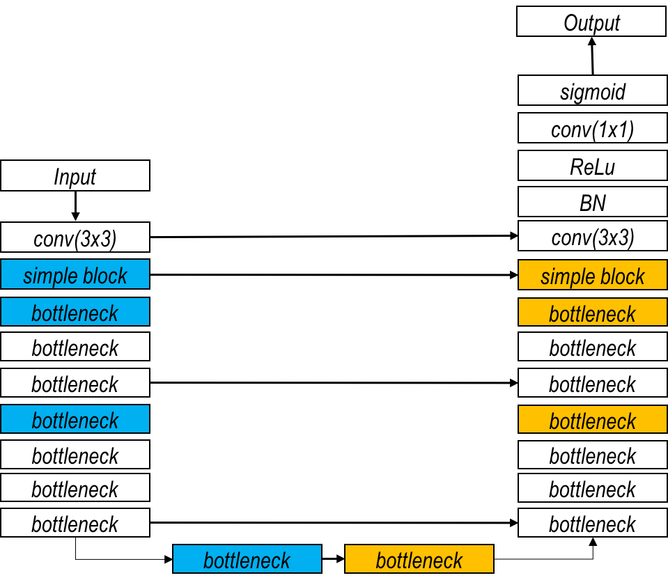
The FC-ResNet model extends ResNets to be fully convolutional by adding an expanding (upsampling) path (Figure 2(a)). Spatial reduction is performed along the contracting path (left) and expansion is performed along the expanding path (right). As in [32] and [38], spatial information lost along the contracting path is recovered in the expanding path by skipping equal resolution features from the former to the latter. Similarly to the identity connections in ResNets, the skipped features coming from the contracting path are summed with the ones in the expanding path.

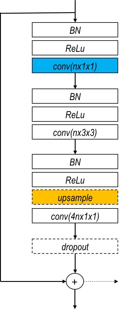
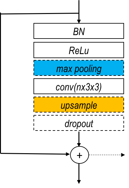
Following the spirit of ResNets, FC-ResNets are composed of two different types of blocks: simple blocks and bottleneck blocks, each composed of at least one batch normalization followed by a non-linearity and one convolution (see Figure 2(b)-2(c)). These blocks can maintain the spatial resolution of their input (marked white in Figure 2(b)-2(c)), perform spatial downsampling (marked blue in Figure 2(b)-2(c)) or spatial upsampling (marked yellow in Figure 2(b)-2(c)). As in ResNets, bottleneck blocks are characterized by their $1\times 1$ convolutions, which are responsible for reducing and restoring the number of feature maps and thus, aim to mitigate the number of parameters of the model.

The detailed description of FC-ResNet architecture used in our pipeline is shown in Table II. The contracting path contains 5 downsampling operations, one $3\times 3$ convolution, one simple block and 21 bottleneck blocks. The contracting path is followed by 3 bottleneck blocks, which precede the expanding path. The expanding path contains 5 upsampling operations, 21 bottleneck blocks, one simple block and one last $3\times 3$ convolution. This FC-ResNet has a total of $11$ millions trainable parameters.

To sum up, our model is composed of a UNet-like model followed by a FC-ResNet. The UNet-like model is composed of 23 convolutional layers and $1.8$ million trainable parameters. Our FC-ResNet has 140 convolutional layers and $11$ millions of trainable parameters. Thus, our full segmentation pipeline has $12.8$ millions of trainable parameters.

Layer Name	Block Type	Output Resolution	Output Width	Repetition Number
Input	-	$512\times 512$	1	-
Down 1	conv $3\times 3$	$512\times 512$	16	2
Pooling 1	maxpooling	$256\times 256$	16	1
Down 2	conv $3\times 3$	$256\times 256$	32	2
Pooling 2	maxpooling	$128\times 128$	32	1
Down 3	conv $3\times 3$	$128\times 128$	64	2
Pooling 3	maxpooling	$64\times 64$	64	1
Down 4	conv $3\times 3$	$64\times 64$	128	2
Pooling 4	maxpooling	$32\times 32$	128	1
Across	conv $3\times 3$	$32\times 32$	256	2
Up 1	upsampling	$64\times 64$	256	1
Merge 1	concatenate	$64\times 64$	384	1
Up 2	conv $2\times 2$	$64\times 64$	128	1
Up 3	conv $3\times 3$	$64\times 64$	128	2
Up 4	upsampling	$128\times 128$	128	1
Merge 2	concatenate	$128\times 128$	192	1
Up 5	conv $2\times 2$	$128\times 128$	64	1
Up 6	conv $3\times 3$	$128\times 128$	64	2
Up 7	upsampling	$256\times 256$	64	1
Merge 3	concatenate	$256\times 256$	96	1
Up 8	conv $2\times 2$	$256\times 256$	32	1
Up 9	conv $3\times 3$	$256\times 256$	32	2
Up 10	upsampling	$512\times 512$	32	1
Merge 4	concatenate	$512\times 512$	48	1
Up 11	conv $2\times 2$	$512\times 512$	16	1
Up 12	conv $3\times 3$	$512\times 512$	16	2
Output	conv $3\times 3$	$512\times 512$	1	1

Table I: Detailed FCN architecture used as a pre-processor in the experiments. Output resolution indicates the spatial resolution of feature maps for an input of size $512\times 512$ and output width represents the feature map dimensionality. Repetition number indicates the number of times the layer is repeated.

Layer Name	Block Type	Output Resolution	Output Width	Repetition Number
Down 1	conv $3\times 3$	$512\times 512$	32	1
Down 2	simple block	$256\times 256$	32	1
Down 3	bottleneck	$128\times 128$	128	3
Down 4	bottleneck	$64\times 64$	256	8
Down 5	bottleneck	$32\times 32$	512	10
Across	bottleneck	$32\times 32$	1024	3
Up 1	bottleneck	$64\times 64$	512	10
Up 2	bottleneck	$128\times 128$	256	8
Up 3	bottleneck	$256\times 256$	128	3
Up 4	simple block	$512\times 512$	32	1
Up 5	conv 3x3	$512\times 512$	32	1
Classifier	conv $1\times 1$	$512\times 512$	1	1

Table II: Detailed FC-ResNet architecture used in the experiments. Output resolution indicates the spatial resolution of feature maps for an input of size $512\times 512$ and output width represents the feature map dimensionality. Repetition number indicates the number of times the block is repeated. For the definition of block types, please refer to Figures 2(b) and 2(c).

III-C Dice Loss

We train our model using the Dice loss ($L_{Dice}$) computed per batch:

$$L_{Dice}=-\frac{2\sum_{i}o_{i}y_{i}}{\sum_{i}o_{i}+\sum_{i}y_{i}},$$ (2)

where $o_{i}\in[0,1]$ represents the $i^{th}$ output of the last network layer (sigmoid output) and $y_{i}\in\{0,1\}$ represents the corresponding ground truth label. Note that the minimum value of the Dice loss is $-1$.

The reason for using the Dice loss over traditional binary crossentropy is two-fold. First, the Dice coefficient is of the common metrics to assess medical image segmentation accuracy, thus, it is natural to optimize it during training. Second, as pointed out in [35], Dice loss is well adapted to the problems with high imbalance between foreground and background classes as it does not require any class frequency balancing.

IV Experiments

In this section, we present experimental results of the proposed pipeline for image segmentation. First, we show that our method achieves state-of-the-art results among all published 2D methods on challenging EM benchmark [5]. Second, we compare our pipeline with standard FCNs [32, 38] and with FC-ResNets [17] on a dataset of CT scans of liver lesions, with 135 manually annotated scans. Finally, we show the normalization effect of the FCN-based pre-processing module on both datasets.

In our experiments, we train with early stopping at the highest Dice value on the validation set with patience of $50$ epochs. We implemented our model in the Keras framework [14] using the Theano backend [3].

IV-A Electron Microscopy dataset

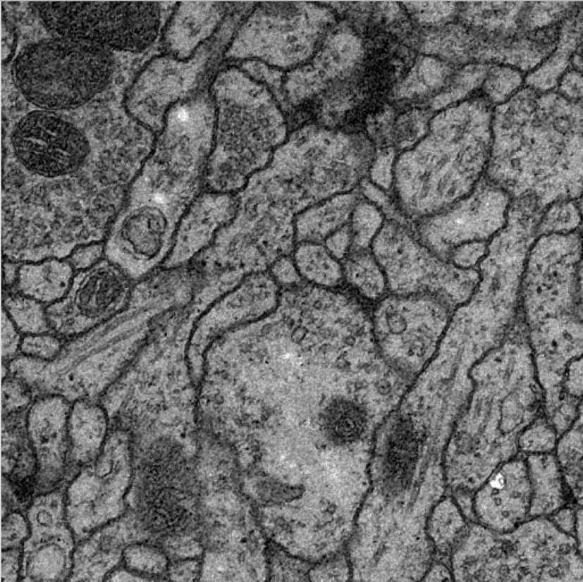
The EM training dataset consists of $30$ images ($512\times 512$ pixels) assembled from serial section transmission electron microscopy of the Drosophila first instar larva ventral nerve cord. The test set is a separate set of $30$ images, for which labels are not provided.

The official metrics used in this dataset are: Maximal foreground-restricted Rand score after thinning ($V_{rand}$) and maximal foreground-restricted information theoretic score after thinning ($V_{info}$) with ($V_{rand}$), being used to order the entries in the leader board. For a detailed description of the metrics, please refer to [5].

During training, we augmented the dataset using random flipping (horizontal and vertical), sheering (with maximal range of $0.41$), rotations (with maximal range of $25$), random cropping ($256\times 256$) and spline warping. We used the same spline warping strategy as [38]. Thus, our data augmentation is similar to the one published in [17]. We trained the model with RMSprop [45] with an initial learning rate of $0.001$, a learning rate decay of $0.001$ and a batch size of $8$. We used weight decay of $0.0001$. For each training, the model with the best validation Dice was stored. In total, we trained 10 models and averaged their outputs at the test time. Each time the model was trained, we randomly split $30$ images into $24$ training images and $6$ validation images.

(a) Input image

(b) FC-ResNet with dropout at test time [17]

(c) Segmentation result of our pipeline

Figure 3: Qualitative segmentation results for EM data. (a) An image from the test set, (b) prediction of FC-ResNet with standarization as a pre-porcessor and dropout at test time and (c) prediction obtained by our pipeline with FCN-based processor followed by FC-ResNet.

Method	$V_{rand}$	$V_{info}$	post-processing	pre-processing	average over	parameters [M]
FusionNet [37]	0.978	0.990	YES	YES	8	31
CUMedVision [13]	0.977	0.989	YES	NO	6	8
Unet [38]	0.973	0.987	NO	YES	7	33
FC-ResNet [17]	0.969	0.986	NO	YES	Dropout	11
Ours	0.981	0.988	NO	NO	10	13

Table III: Comparison to published FCN results for EM dataset. $V_{rand}$ is the measure used to rank the submissions. For full ranking of all submitted methods please refer to the challenge website: http://brainiac2.mit.edu/isbi_challenge/leaders-board-new.

Method	$V_{rand}$	$V_{info}$	2D/3D
IAL [6]	0.980	0.988	2D
FusionNet [37]	0.978	0.990	2D
CUMedVision [13]	0.977	0.989	2D
Unet [38]	0.973	0.987	2D
IDSIA [16]	0.970	0.985	2D
motif [49]	0.972	0.985	2D
SCI [31]	0.971	0.982	3D
optree-idsia[46]	0.970	0.985	2D
FC-ResNet [17]	0.969	0.986	2D
PyraMiD-LSTM[41]	0.968	0.983	3D
Ours	0.981	0.988	2D

Table IV: Comparison to published entries for EM dataset. $V_{rand}$ is the measure used to order the submissions. For full ranking of all submitted methods please refer to the challenge website: http://brainiac2.mit.edu/isbi_challenge/leaders-board-new.

The comparison of our method to other FCNs is shown in Table III. Our pipeline outperforms all other fully convolutional approaches when looking at the primary metric ($V_{rand}$ score), improving it by 0.003 over the second best fully convolutional approach (FusionNet [37]). When comparing our pipeline (FCN pre-processing followed by FC-ResNet) to the pipeline of [17] (standardization pre-processing followed by FC-ResNet), we observe a significant increase in performance. The same happens when comparing our pipeline to FusionNet [37] (rescaling pre-processing followed by FC-ResNet). It is worth noting that FusionNet applies intensity shifts with Gaussian noise as data augmentation to account for input variability. All these results suggest that FC-ResNet is better complemented by an FCN pre-processor than by traditional pre-processors such as standardization or rescaling. It is worth noting that our pipeline has only slightly more parameters than [17] and significantly fewer parameters than [37]. There are two additional fully convolutional approaches submitted for this dataset: UNet [38] and CUMedVision [13], the latter being based on FCN8 [32]. The pre-processing used on this dataset varies from range normalization to values from 0 to 1 [37] to data standardization [17]. For post-processing, median filter [37] and watershed algorithm [13] are used. All methods use either prediction or model averaging at test time.

Table IV compares our method to other published entries for EM dataset. As shown in the table, we report the highest $V_{rand}$ score (at the moment of writing the paper), when compared to all published 2D methods. The second best entry is IAL [6], which introduces a graph-cut post-processing method to refine FCN predictions. In [6], a 2D approach was tested resulting in $0.980$ $V_{rand}$ score and $0.988$ $V_{info}$ score. However, IAL leaderboard entrance incorporates 3D context information and achieves an improvement of $0.003$ in $V_{rand}$ score and $0.001$ in $V_{info}$ score w.r.t. IAL 2D entry.

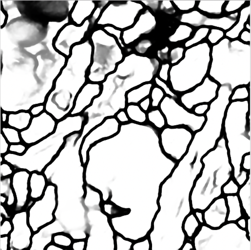
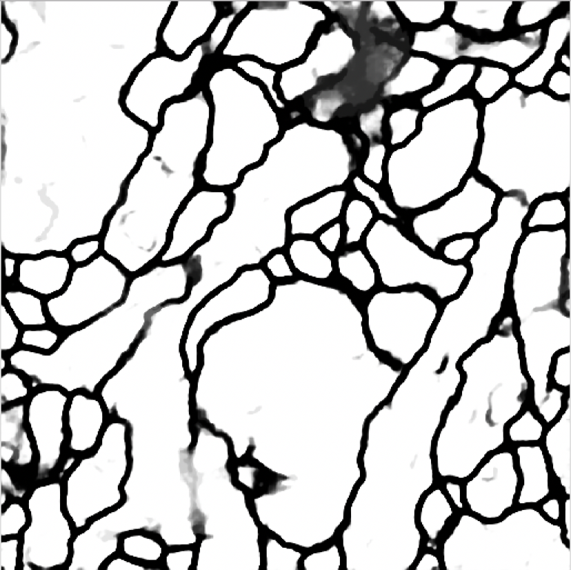
Finally, we show some qualitative analysis of our method in Figure 3, where we display a prediction of a single test frame for two different pipelines: FC-ResNet from [17] in Figure 3(b) and of our pipeline in Figure 3(c). The white color in the prediction images correspond to the cell class and the black color correspond to the cell membrane class. The different degrees of gray correspond to regions in which the model is (more or less) uncertain about the class assignment. The difference is especially visible when comparing our model to FC-ResNet, we can see that the predictions are sharper and clearer, suggesting that the FCN-pre-processor has properly prepared the image for FC-ResNet.

IV-B Liver lesion dataset

Our in-house dataset consists of abdominal contrast-enhanced CT-scans from patients diagnosed with colorectal metastases (CRM). All images are $512\times 512$ with a pixel size varying from $0.53$ to $1.25$ mm and a slice thickness varying from $0.5$ to $5.01$ mm. The pixel intensities vary between $-3000$ and $1500$. For each volume, CRM were segmented manually using MITK Workbench [1] by medical students and reviewed by professional image analysts, resulting in 135 CT scans with manually segmented CRM. In addition to that, manual liver segmentation was provided for 58 of the 135 CT scans. This data was collected with the specific goal of segmenting lesions only within the liver.

We split the dataset to have $77$ training images with CRM segmented, $28$ validation images with liver and CRM segmented and 30 test images with liver and CRM segmented. Note that for the training set we do not have liver segmentations available. The liver segmentations of both the validation and the test sets are used to limit the lesion segmentation evaluation only to the liver, treating the rest of the image as a void class.

During the training, we randomly crop a 2D $128\times 128$ pixel patch containing CRM from a CT scan. We train the model with RMSprop [45] with an initial learning rate of $0.001$ and a learning rate decay of $0.001$. We use weight decay of $0.0001$ in the pre-processor and $0.0005$ in FC-ResNet.

Method	parameters [M]	Validation			Test
		loss	$Dice_{lesion}$	$Dice_{liver}$	loss	$Dice_{lesion}$	$Dice_{liver}$
FCN8 [32]	128	-0.419	0.589	0.994	-0.437	0.535	0.989
Unet [38]	33	-0.451	0.553	0.994	-0.396	0.570	0.990
FC-ResNet [17]	11	-0.223	0.551	0.993	-0.224	0.617	0.990
Ours	13	-0.795	0.771	0.997	-0.796	0.711	0.993

Table V: Results on the liver lesion dataset for both validation and test sets.

We follow the same training procedure for all FCN methods: FCN8 [32], UNet [38] and FC-ResNets [17]. Results are reported in Table V. All models were trained with the Dice loss with batch size of $20$ at training time and $1$ at validation and test time. Our approach outperforms other methods on this challenging dataset, achieving the best validation loss of $-0.795$ and lesion validation Dice of $0.771$. The second best validation loss was obtained by the UNet model ($-0.451$) and the second best lesion validation Dice was obtained by the FCN8 model ($0.589$). Moreover, our model generalizes well on test set reaching a loss of $-0.796$ and a Dice of $0.711$.

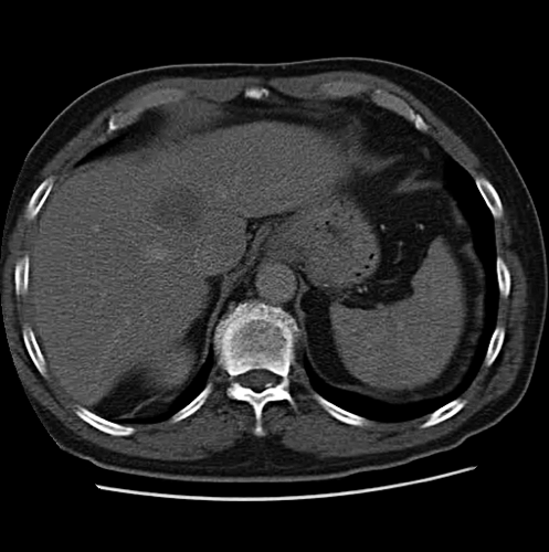
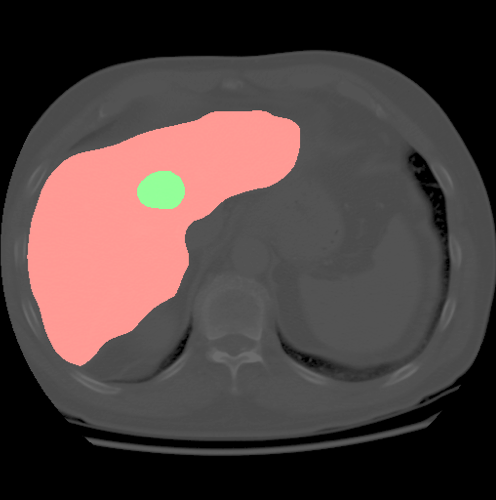
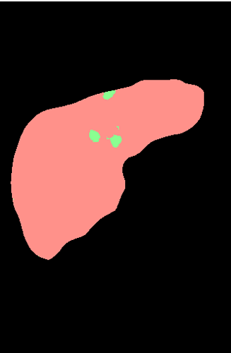
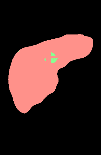
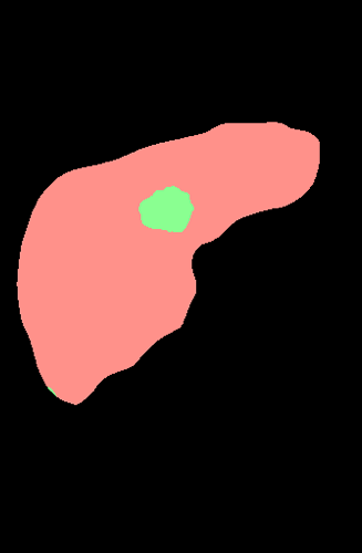
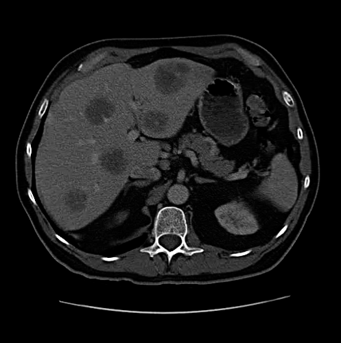
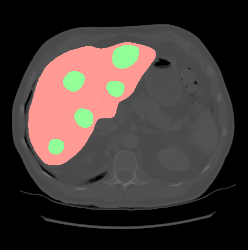
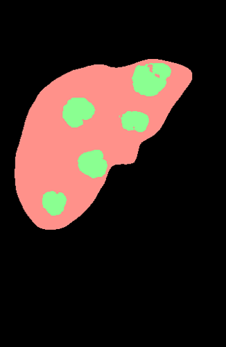
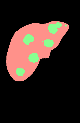
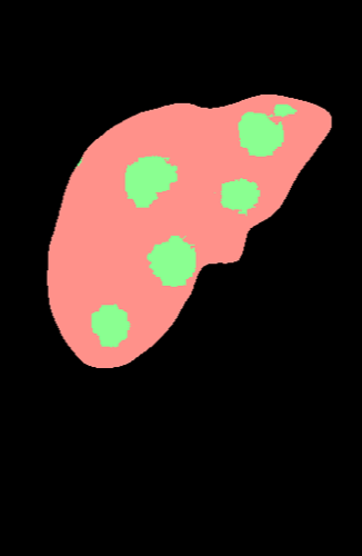
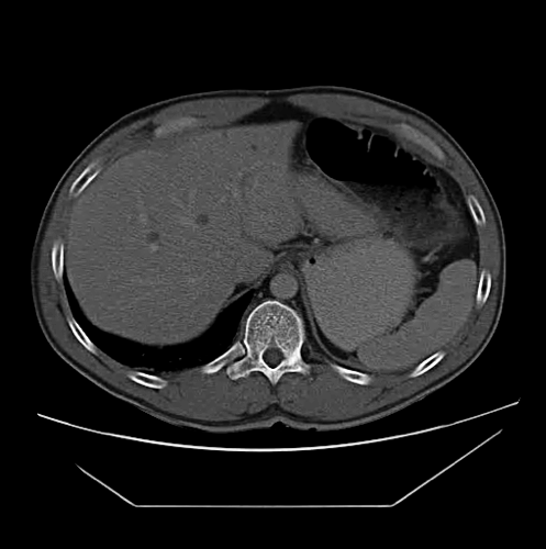
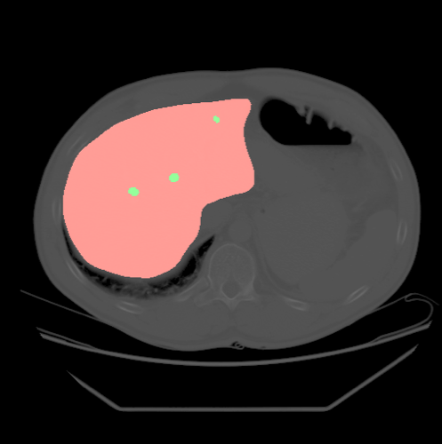
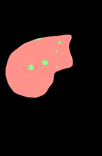
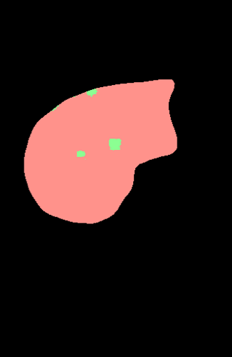
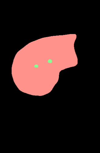
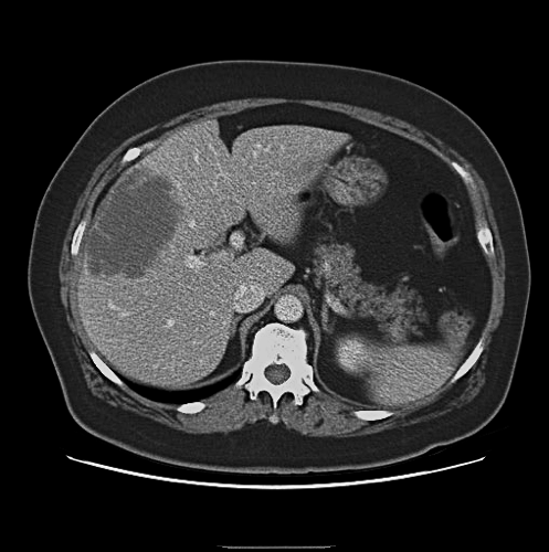
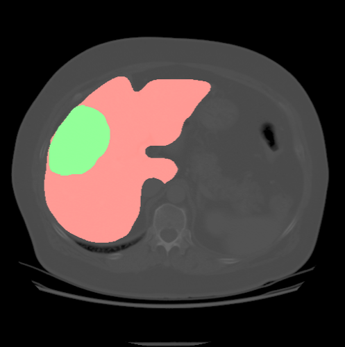
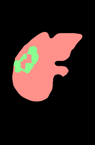
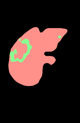
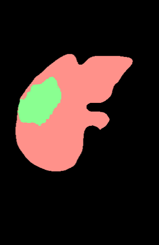
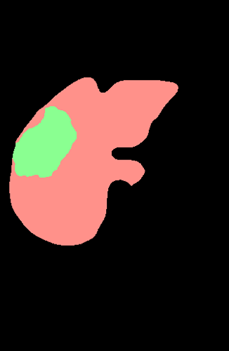
Finally, we show some qualitative results for liver lesion segmentation in Figure 4, obtained without any user interaction or manual intialization. Figure 4() displays sample input CT images to segment, Figure 4() shows ground truth annotations and Figures 4() to 4() present predictions of FCN8, UNet, FC-ResNet and of our approach respectively. Our approach performs better for all types of lesions: small lesions (see third row in Figure 4), medium size lesions (see first and second rows in Figure 4) and large lesions (see forth row in Figure 4). Furthermore, the lesion segmentation is better adjusted to ground truth annotation, has less false positives and does not have unsegmented holes or gaps within the lesions.

() Input CT image

() Ground Truth

() FCN8

() Unet

() FC-ResNet

() Ours

Figure 4: Qualitative results on test set for the liver lesion dataset. Each line displays an example form the test set. From left to right: (a) represents an image, (b) displays the expert annotation of liver (red) and lesion (green), (c) displays a prediction for FCN8 model, (d) displays a prediction for UNet model, (e) displays a prediction for FC-ResNet model and (f) displays a prediction of our method.

IV-C Prostate dataset

The final experiment tested the segmentation framework on T2-w MR images of the prostate provided by the PROMISE12 challenge. The training dataset contains 50 T2-w MR images of the prostate together with segmentation masks. The test set consists of 30 MR images for which the ground truth is held out by the organizer for independent evaluation. These MRIs are acquired in different hospitals, using different equipments, different acquisition protocols and include both patients with benign disease (e.g. benign prostatic hyperplasia) as well as with prostate cancer. Thus, the dataset variations include: voxel size, dynamic range, position, field of view and anatomic appearance. Contrary to all previously published methods we did not apply any pre-processing step nor volume resizing at training or testing time.

During training, we augmented the dataset using random sheering (with maximal range of $0.1$), rotations (with maximal range of $10$), random cropping ($256\times 256$) and spline warping. We trained the model with RMSprop [45] with an initial learning rate of $0.0004$, a learning rate decay of $0.001$ and a batch size of $24$. We used weight decay of $0.00001$. For each training, the model with the best validation Dice was stored. In total, we trained 10 models and averaged their outputs at the test time. Each time the model was trained, we randomly split $50$ training volumes into $40$ training images and $10$ validation images. Because the method is still based on 2D images, a connected component method was applied on the output to select the largest structure on each volume.

Method	Score [-]	Dice [%]	Avg. Dist. [mm]	Vol. Diff. [%]
2D FCNs
Ours	83.02	87.4	2.17	12.37
SITUS	79.92	84.13	2.96	23.00
3D FCNs
CUMED [50]	86.65	89.43	1.95	6.95
CAMP-TUM2 [35]	82.39	86.91	2.23	14.98
SRIBHME	74.17	74.46	2.83	34.89

Table VI: Comparison to the automatic entries based on FCNs for the prostate dataset. For full ranking of all submitted methods please refer to the challenge website: https://grand-challenge.org/site/promise12/results/.

Overall, for our method the Dice coefficient is of $87.4$ on the entire gland, with an average boundary distance of $2.17$mm and a volume difference of $12.37\%$. The comparison to other FCNs on the prostate data is shown in Table VI. In comparison, we use the score provided by the challenge organizer. As it can be seen, our pipeline outperforms other method based on 2D FCNs and is competitive with methods based on 3D FCNs.

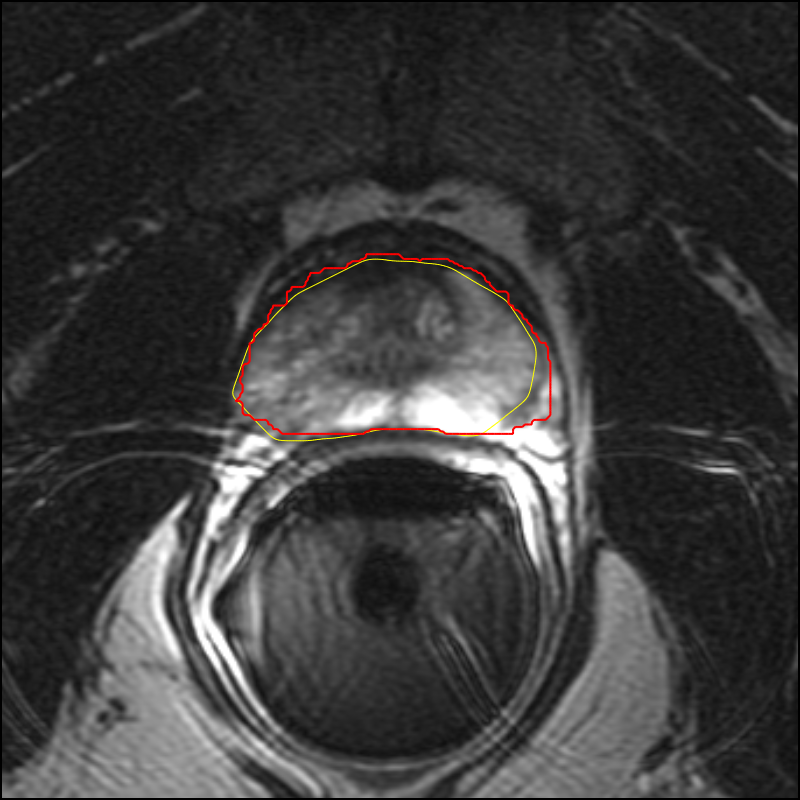
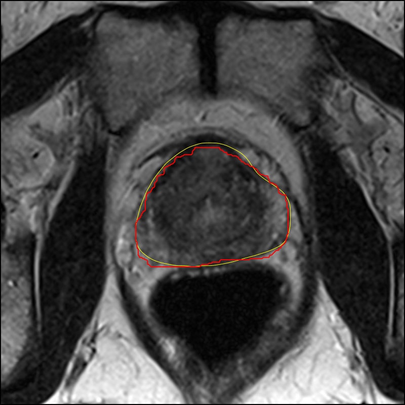
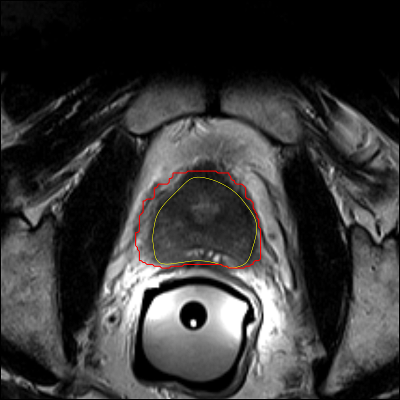
Figure 5 shows some qualitative results. The prostate segmentations are well adjusted to ground truth annotations and do not have unsegmented holes or gaps within the prostate. Due to the lack of 3D context information, our method, in some cases, is over-segmenting the base of the apex of the prostate (e.g. see Figure 5). These results rank amongst the best automated approaches for prostate segmentation and without tedious and application specific pre-processing steps.

Figure 5: Qualitative results of our pipeline on the test set. The yellow line shows ground truth annotations while the red line displays our prediction. For more examples of qualitative results please refer to https://grand-challenge.org/site/promise12/resultpro/?id=UdeM2D&folder=20170201000157_2703_UdeM2D_Result

IV-D Data normalization

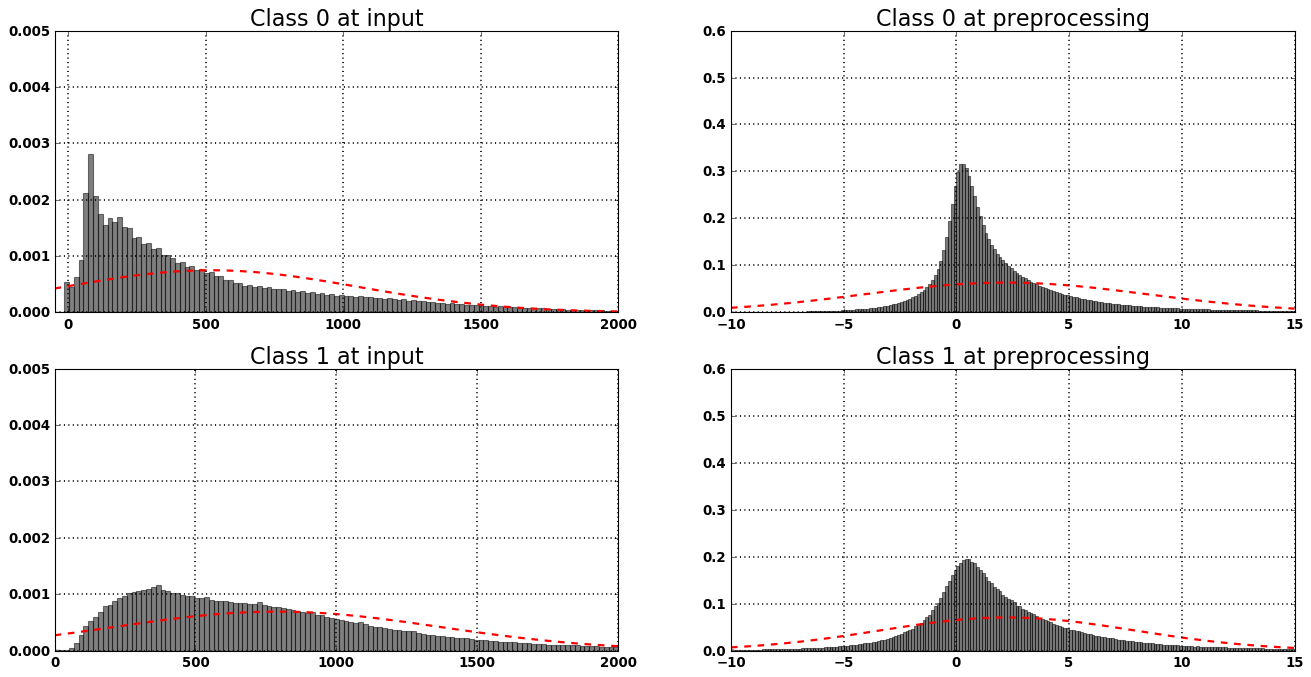
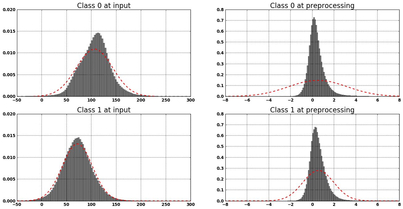
In this subsection, we provide a more detailed analysis on the trained models. In particular, we investigate the effect of an FCN-based pre-processor on the data distribution. The distribution of validation set pixel intensities at the input of our pipeline (input to FCN-based pre-processor) and at the input of the FC-ResNet are shown in Figure 6. Together with intensity histograms, we plot the normal distribution fitting the validation data (dashed red line).

Figure 6(a) shows the plots for prostate data, where class 0 represent background and class 1 represent prostate. We observe that intensities are shifted from $[0,2000]$ at the FCN input to $[-5,10]$ at the FC-ResNet input. For liver lesion dataset, we only plot the distributions for liver (referred to as class 0) and lesion (referred to as class 1), ignoring the distribution of regions outside of the liver. The liver distributions are shown in Figure 6(b). We observe similar behavior as for the prostate data: intensities are shifted from $[0,200]$ at the FCN input to $[-2,3]$ at the FC-ResNet input.

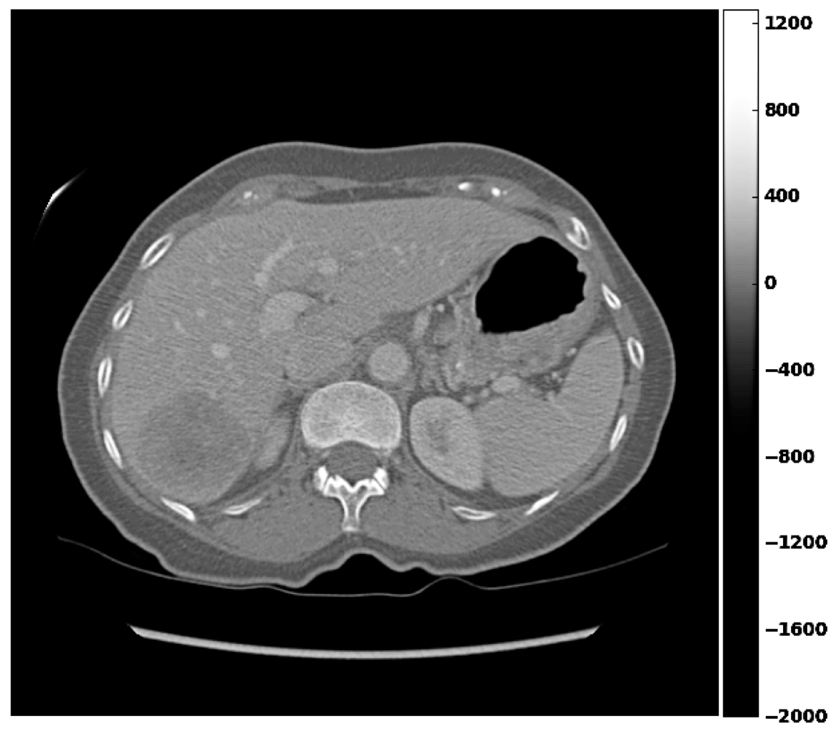
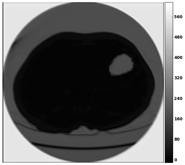
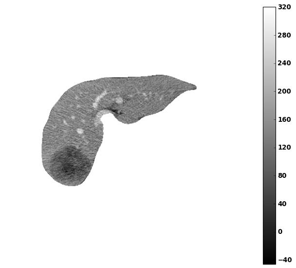
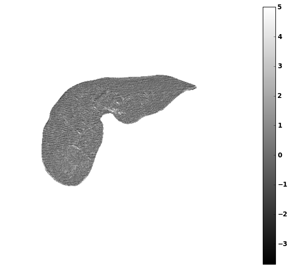
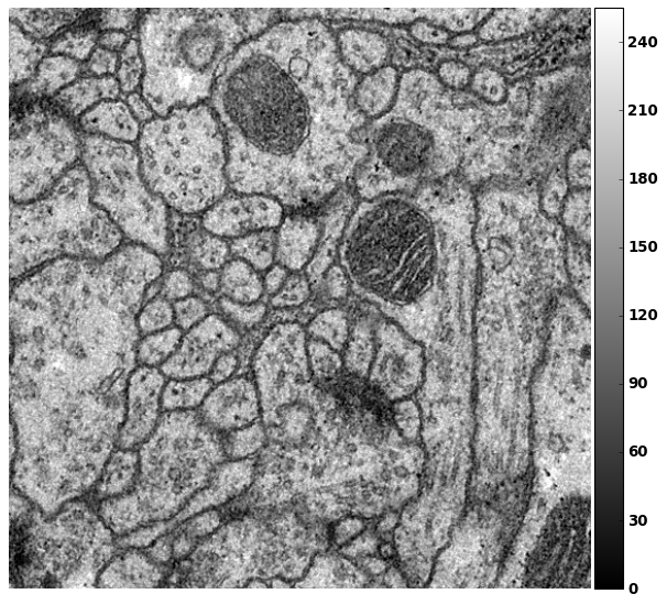
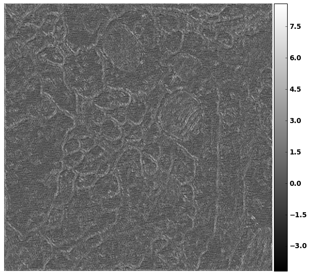
The qualitative evaluation of the FCN-based pre-processor is displayed in Figures 7 and 8 for liver and EM data, respectively. Figure 7 shows visualizations of how a liver image is transformed from the input of our pre-processor (Figure 7(a)) to its output (Figure 7(b)). Analogously, Figures 7(c) and 7(d) emphasize how intensities within the liver change, by removing the void pixels of the image. Note that the FCN-based pre-processor does not perform any pre-segmentation of the lesion, i.e. the lesion is not more visible on the pre-processed image (Figure 7(c) than at the input (Figure 7(d))). This suggests that the FCN is only normalizing the data to values that are adequate for iterative refinement that happens within the FC-ResNet model. Similar observations can be made for EM data, which is displayed in Figure 8.

(a) Prostate dataset

(b) Liver lesion dataset

Figure 6: Intensity distribution histograms for (a) Prostate dataset and (b) liver lesion dataset. The plots represent the following information: (left-up subfigure) the 0-class distribution of input pixels, (left-bottom subfigure) the 1-class distribution for input pixels, (right-up subfigure) the 0-class distribution after FCN pre-processing, (right-bottom subfigure) the 1-class distribution after pre-processing. The red dashed-line represents normal distribution fitted to the data.

(a) Input image

(b) Pre-procesor output

(c) Image cropped to liver

(d) Pre-procesor output cropped to liver

Figure 7: Visualization of the output of the pre-processor module for liver lesion dataset.

(a) Input image

(b) Pre-procesor output

Figure 8: Visualization of the output of the pre-processor module for the EM dataset.

V Discussion & Conclusion

In this paper, we have introduced a simple, yet powerful segmentation pipeline for medical images that combines fully convolutional networks with fully convolutional ResNets. Our pipeline is built from a low-capacity FCN model followed by a very deep FC-ResNet (more than 100 layers). We have highlighted the importance of pre-processing when using FC-ResNets and shown that a low-capacity FCN model can serve as a pre-processor to normalize raw medical image data. We argued that FC-ResNets are better complemented by the proposed FCN pre-processor than by traditional pre-processors, given the normalization they achieve. Finally, we have shown that using this pipeline we exhibit state-of-the-art performance on the challenging EM benchmark, improve segmentation results on our in-house liver lesion dataset, when compared to standard FCN methods and yield competitive results on challenging 3D MRI prostate segmentation task. These results illustrate the strong potential and versatility of the framework by achieving highly accurate results on multi-modality images from different anatomical regions and organs.

The fact that FC-ResNets require some kind of data pre-processing is not very surprising, given the model construction. The identity path forwards the input data right to the output, while applying small transformations along the residual path. These small transformations are controlled by batch normalization. This input-forwarding especially affects medical imaging data, where the pixel intensities range is much broader than in standard RGB images. Therefore, adequate pre-processing becomes crucial for FC-ResNets to achieve significant improvement over standard FCN approaches, especially for some imaging modalities with greater variability in acquisition protocols. Standard FCNs do not contain the identity path and, thus, are more robust to the input data distribution. However, the lack of this identity path affects the optimization process and limits the depth of the tested models.

In light of recent advancements in understanding both CNNs and ResNets, our pipeline can have two possible interpretations. On one hand, the pipeline could be explained as having the FCN model working as a pre-processor followed by the FC-ResNet model performing the task of an ensemble of relatively shallow models, leading to a robust classifier. On the other hand, the interpretation of our pipeline could revolve around the iterative inference point of view of ResNets [20]. In this scenario, the role of the FCN would be to produce an input proposal that would be iteratively refined by the FC-ResNet to generate the proper segmentation map. It is worth noting that, in both interpretations, FC-ResNets should be relatively deep (hundreds of layers) in order to take full advantage of the ensemble of shallow networks or iterative refinement of the initial proposal. FC-ResNets might not have been deep enough in many medical image segmentation pipelines to achieve these effects.

Potential future direction might involve experimentation with different variants of architectures that could serve as a pre-processor. This architecture exploration should not be limited to FCN-like models. From medical image segmentation perspective, the model could potentially benefit by expanding it to 3D FCN.

References

- [1] The medical imaging interaction toolkit (mitk). http://mitk.org/wiki/The_Medical_Imaging_Interaction_Toolkit_(MITK).
- [2] Isbi 2013 challenge: 3d segmentation of neurites in em images. http://brainiac2.mit.edu/SNEMI3D/home, 2013.
- [3] R. Al-Rfou, G. Alain, A. Almahairi, and et al. Theano: A python framework for fast computation of mathematical expressions. CoRR, abs/1605.02688, 2016.
- [4] S. Andermatt, S. Pezold, and P. Cattin. Multi-dimensional Gated Recurrent Units for the Segmentation of Biomedical 3D-Data, pages 142–151. Springer International Publishing, Cham, 2016.
- [5] I. Arganda-Carreras, S. C. Turaga, D. R. Berger, et al. Crowdsourcing the creation of image segmentation algorithms for connectomics. Frontiers in Neuroanatomy, 9(142), 2015.
- [6] T. Beier, B. Andres, U. Köthe, and F. A. Hamprecht. An Efficient Fusion Move Algorithm for the Minimum Cost Lifted Multicut Problem, pages 715–730. Springer International Publishing, Cham, 2016.
- [7] A. Ben-Cohen, I. Diamant, E. Klang, M. Amitai, and H. Greenspan. Fully convolutional network for liver segmentation and lesions detection. In Deep Learning and Data Labeling for Medical Applications, In Conjunction with MICCAI 2016, Athens, Greece, October 21, 2016, Proceedings, pages 77–85, 2016.
- [8] A. Birenbaum and H. Greenspan. Longitudinal multiple sclerosis lesion segmentation using multi-view convolutional neural networks. In Deep Learning and Data Labeling for Medical Applications, In Conjunction with MICCAI 2016, Athens, Greece, October 21, 2016, Proceedings, pages 58–67, 2016.
- [9] A. Casamitjana, S. Puch, A. Aduriz, E. Sayrol, and V. Vilaplana. 3d convolutional networks for brain tumor segmentation. In Proceedings of the MICCAI Challenge on Multimodal Brain Tumor Image Segmentation (BRATS) 2016, pages 65–68, 2016.
- [10] K. H. Cha, L. Hadjiiski, R. K. Samala, et al. Urinary bladder segmentation in ct urography using deep-learning convolutional neural network and level sets. Medical Physics, 43(4):1882–1896, 2016.
- [11] P. D. Chang. Fully convolutional neural networks with hyperlocal features for brain tumor segmentation. In Proceedings of the MICCAI Challenge on Multimodal Brain Tumor Image Segmentation (BRATS) 2016, pages 4–9, 2016.
- [12] H. Chen, Q. Dou, L. Yu, and P. Heng. Voxresnet: Deep voxelwise residual networks for volumetric brain segmentation. CoRR, abs/1608.05895, 2016.
- [13] H. Chen, X. Qi, J. Cheng, and P. A. Heng. Deep contextual networks for neuronal structure segmentation. In Proceedings of the 13th AAAI Conference on Artificial Intelligence, February 12-17, 2016, Phoenix, Arizona, USA., pages 1167–1173, 2016.
- [14] F. Chollet. Keras. https://github.com/fchollet/keras, 2015.
- [15] P. F. Christ, M. E. A. Elshaer, F. Ettlinger, et al. Automatic liver and lesion segmentation in CT using cascaded fully convolutional neural networks and 3d conditional random fields. CoRR, abs/1610.02177, 2016.
- [16] D. Ciresan, A. Giusti, L. M. Gambardella, and J. Schmidhuber. Deep neural networks segment neuronal membranes in electron microscopy images. In NIPS 25, pages 2843–2851. Curran Associates, Inc., 2012.
- [17] M. Drozdzal, E. Vorontsov, G. Chartrand, S. Kadoury, and C. Pal. The importance of skip connections in biomedical image segmentation. CoRR, abs/1608.04117, 2016.
- [18] A. Fakhry, T. Zeng, and S. Ji. Residual deconvolutional networks for brain electron microscopy image segmentation. IEEE Transactions on Medical Imaging, PP(99):1–1, 2016.
- [19] I. Goodfellow, Y. Bengio, and A. Courville. Deep learning. Book in preparation for MIT Press, 2016.
- [20] K. Greff, R. K. Srivastava, and J. Schmidhuber. Highway and residual networks learn unrolled iterative estimation. openreview, -, 2016.
- [21] M. Havaei, A. Davy, D. Warde-Farley, et al. Brain tumor segmentation with deep neural networks. CoRR, abs/1505.03540, 2015.
- [22] M. Havaei, N. Guizard, H. Larochelle, and P. Jodoin. Deep learning trends for focal brain pathology segmentation in MRI. CoRR, abs/1607.05258, 2016.
- [23] K. He, X. Zhang, S. Ren, and J. Sun. Deep residual learning for image recognition. CoRR, abs/1512.03385, 2015.
- [24] K. He, X. Zhang, S. Ren, and J. Sun. Identity mappings in deep residual networks. CoRR, abs/1603.05027, 2016.
- [25] G. Huang, Y. Sun, Z. Liu, D. Sedra, and K. Q. Weinberger. Deep networks with stochastic depth. CoRR, abs/1603.09382, 2016.
- [26] S. Ioffe and C. Szegedy. Batch normalization: Accelerating deep network training by reducing internal covariate shift. CoRR, abs/1502.03167, 2015.
- [27] K. Kamnitsas, C. Ledig, V. F. J. Newcombe, et al. Efficient multi-scale 3d CNN with fully connected CRF for accurate brain lesion segmentation. CoRR, abs/1603.05959, 2016.
- [28] P. Krähenbühl and V. Koltun. Efficient inference in fully connected crfs with gaussian edge potentials. In J. Shawe-Taylor, R. S. Zemel, P. L. Bartlett, F. Pereira, and K. Q. Weinberger, editors, Advances in Neural Information Processing Systems 24, pages 109–117. Curran Associates, Inc., 2011.
- [29] W. Li, F. Jia, and Q. Hu. Automatic segmentation of liver tumor in ct images with deep convolutional neural networks. Journal of Computer and Communication, 3(11).
- [30] Q. Liao and T. A. Poggio. Bridging the gaps between residual learning, recurrent neural networks and visual cortex. CoRR, abs/1604.03640, 2016.
- [31] T. Liu, C. Jones, M. Seyedhosseini, and T. Tasdizen. A modular hierarchical approach to 3d electron microscopy image segmentation. Journal of Neuroscience Methods, 226:88 – 102, 2014.
- [32] J. Long, E. Shelhamer, and T. Darrell. Fully convolutional networks for semantic segmentation. CVPR (to appear), Nov. 2015.
- [33] T. K. Lun and W. Hsu. Brain tumor segmentation using deep convolutional neural network. In Proceedings of the MICCAI Challenge on Multimodal Brain Tumor Image Segmentation (BRATS) 2016, pages 26–29, 2016.
- [34] R. McKinley, R. Wiest, and M. Reyes. Nabla-net: a deep dag-like convolutional architecture for biomedical image segmentation: application to high- and low-grade glioma segmentation. In Proceedings of the MICCAI Challenge on Multimodal Brain Tumor Image Segmentation (BRATS) 2016, pages 1–4, 2016.
- [35] F. Milletari, N. Navab, and S. Ahmadi. V-net: Fully convolutional neural networks for volumetric medical image segmentation. CoRR, abs/1606.04797, 2016.
- [36] B. Pandian1, J. Boyle1, and D. A. Orringer1. Multimodal tumor segmentation with 3d volumetric convolutional neural networks. In Proceedings of the MICCAI Challenge on Multimodal Brain Tumor Image Segmentation (BRATS) 2016, pages 1–4, 2016.
- [37] T. M. Quan, D. G. C. Hildebrand, and W.-K. Jeong. FusionNet: A deep fully residual convolutional neural network for image segmentation in connectomics. ArXiv e-prints, Dec. 2016.
- [38] O. Ronneberger, P. Fischer, and T. Brox. U-net: Convolutional networks for biomedical image segmentation. CoRR, abs/1505.04597, 2015.
- [39] H. R. Roth, L. Lu, A. Farag, H. Shin, J. Liu, E. Turkbey, and R. M. Summers. Deeporgan: Multi-level deep convolutional networks for automated pancreas segmentation. CoRR, abs/1506.06448, 2015.
- [40] N. Srivastava, G. Hinton, A. Krizhevsky, I. Sutskever, and R. Salakhutdinov. Dropout: A simple way to prevent neural networks from overfitting. J. Mach. Learn. Res., 15(1):1929–1958, Jan. 2014.
- [41] M. F. Stollenga, W. Byeon, M. Liwicki, and J. Schmidhuber. Parallel multi-dimensional lstm, with application to fast biomedical volumetric image segmentation. CoRR, abs/1506.07452, 2015.
- [42] M. Styner, J. Lee, B. Chin, et al. 3d segmentation in the clinic: A grand challenge ii: Ms lesion segmentation. 11 2008.
- [43] C. Szegedy, W. Liu, Y. Jia, et al. Going deeper with convolutions. CoRR, abs/1409.4842, 2014.
- [44] W. Thong, S. Kadoury, N. Piché, and C. J. Pal. Convolutional networks for kidney segmentation in contrast-enhanced ct scans. Computer Methods in Biomechanics and Biomedical Engineering: Imaging & Visualization, pages 1–6, 2016.
- [45] T. Tieleman and G. Hinton. Lecture 6.5—RmsProp: Divide the gradient by a running average of its recent magnitude. COURSERA: Neural Networks for Machine Learning, 2012.
- [46] M. G. Uzunbaş, C. Chen, and D. Metaxsas. Optree: A Learning-Based Adaptive Watershed Algorithm for Neuron Segmentation, pages 97–105. Springer International Publishing, Cham, 2014.
- [47] A. Veit, M. J. Wilber, and S. J. Belongie. Residual networks are exponential ensembles of relatively shallow networks. CoRR, abs/1605.06431, 2016.
- [48] R. Vivanti, A. Ephrat, L. Joskowicz, N. Lev-Cohain, O. A. Karaaslan, and J. Sosna. Automatic liver tumor segmentation in follow-up CT scans: Preliminary method and results. In Patch-MI 2015, Held in Conjunction with MICCAI 2015, Munich, Germany, October 9, 2015, pages 54–61, 2015.
- [49] X. Wu. An iterative convolutional neural network algorithm improves electron microscopy image segmentation. CoRR, abs/1506.05849, 2015.
- [50] L. Yu, X. Yang, H. Chen, J. Qin†, and P.-A. Heng. Volumetric convnets with mixed residual connections for automated prostate segmentation from 3d mr images. In Proceedings of AAAI, 2017.
- [51] M. D. Zeiler and R. Fergus. Visualizing and understanding convolutional networks. CoRR, abs/1311.2901, 2013.
- [52] X. Zhao, Y. Wu, G. Song, Z. Li, Y. Fan, and Y. Zhang. Brain tumor segmentation using a fully convolutional neural network with conditional random elds. In Proceedings of the MICCAI Challenge on Multimodal Brain Tumor Image Segmentation (BRATS) 2016, pages 77–80, 2016.
- [53] Y. Zheng, D. Liu, B. Georgescu, D. Xu, and D. Comaniciu. Deep learning based automatic segmentation of pathological kidney in ct: Local vs. global image context. In L. Lu, Y. Zheng, G. Carneiro, and L. Yang, editors, Deep Learning and Convolutional Neural Networks for Medical Image Computing. Springer, 2016.