Exact Diffusion for Distributed Optimization and Learning — Part I: Algorithm Development
Abstract
This work develops a distributed optimization strategy with guaranteed exact convergence for a broad class of left-stochastic combination policies. The resulting exact diffusion strategy is shown in Part II [2] to have a wider stability range and superior convergence performance than the EXTRA strategy. The exact diffusion solution is applicable to non-symmetric left-stochastic combination matrices, while many earlier developments on exact consensus implementations are limited to doubly-stochastic matrices; these latter matrices impose stringent constraints on the network topology. The derivation of the exact diffusion strategy in this work relies on reformulating the aggregate optimization problem as a penalized problem and resorting to a diagonally-weighted incremental construction. Detailed stability and convergence analyses are pursued in Part II [2] and are facilitated by examining the evolution of the error dynamics in a transformed domain. Numerical simulations illustrate the theoretical conclusions.
Index Terms:
distributed optimization, diffusion, consensus, exact convergence, left-stochastic matrix, doubly-stochastic matrix, balanced policy, Perron vector.I Introduction and Motivation
This work deals with deterministic optimization problems where a collection of networked agents operate cooperatively to solve an aggregate optimization problem of the form:
| (1) |
In this formulation, each risk function is convex and differentiable, while the aggregate cost is strongly-convex. Throughout the paper, we assume the network is undirected. All agents seek to determine the unique global minimizer, , under the constraint that agents can only communicate with their neighbors. This distributed approach is robust to failure of links and/or agents and scalable to the network size. Optimization problems of this type find applications in a wide range of areas including wireless sensor networks [3, 4, 5, 6], multi-vehicle and multi-robot control systems [7, 8], cyber-physical systems and smart grid implementations [9, 10, 11, 12], distributed adaptation and estimation [13, 14, 15, 16, 17], distributed statistical learning [18, 19, 20] and clustering [21, 22].
There are several classes of distributed algorithms that can be used to solve problem (1). In the primal domain, implementations that are based on gradient-descent methods are effective and easy to implement. There are at least two prominent variants under this class: the consensus strategy [23, 24, 25, 26, 27, 28, 29, 30] and the diffusion strategy [13, 14, 15, 16, 17]. There is a subtle but critical difference in the order in which computations are performed under these two strategies. In the consensus implementation, each agent runs a gradient-descent type iteration, albeit one where the starting point for the recursion and the point at which the gradient is approximated are not identical. This construction introduces an asymmetry into the update relation, which has some undesirable instability consequences (described, for example, in Secs. 7.2–7.3, Example 8.4, and also in Theorem 9.3 of [14] and Sec. V.B and Example 20 of [13]). The diffusion strategy, in comparison, employs a symmetric update where the starting point for the iteration and the point at which the gradient is approximated coincide. This property results in a wider stability range for diffusion strategies [13, 14]. Still, when sufficiently small step-sizes are employed to drive the optimization process, both types of strategies (consensus and diffusion) are able to converge exponentially fast, albeit only to an approximate solution [14, 27]. Specifically, it is proved in [14, 31, 27] that both the consensus and diffusion iterates under constant step-size learning converge towards a neighborhood of square-error size around the true optimizer, , i.e., as , where denotes the step-size and denotes the error at agent and iteration relative to . Since we are dealing with deterministic optimization problems, this small limiting bias is not due to any gradient noise arising from stochastic approximations; it is instead due to the inherent structure of the consensus and diffusion updates as clarified in the sequel.
Another important family of distributed algorithms are those based on the distributed alternating direction method of multipliers (ADMM) [32, 33, 34] and its variants [35, 36, 37]. These methods treat problem (1) in both the primal and dual domains. It is shown in [34] that distributed ADMM with constant parameters will converge exponentially fast to the exact global solution . However, distributed ADMM solutions are computationally more expensive since they necessitate the solution of optimal sub-problems at each iteration. Some useful variations of distributed ADMM [35, 36, 37] may alleviate the computational burden, but their recursions are still more difficult to implement than consensus or diffusion.
In more recent work [38], a modified implementation of consensus iterations, referred to as EXTRA, is proposed and shown to converge to the exact minimizer rather than to an neighborhood around . The modification has a similar computational burden as traditional consensus and is based on adding a step that combines two prior iterates to remove bias. Motivated by [38], other variations with similar properties were proposed in [39, 40, 41, 42, 43]. These variations rely instead on combining inexact gradient evaluations with a gradient tracking technique. The resulting algorithms, compared to EXTRA, have two information combinations per recursion, which doubles the amount of communication variables compared to EXTRA, and can become a burden when communication resources are limited.
The current work is motivated by the following considerations. The result in [38] shows that the EXTRA technique resolves the bias problem in consensus implementations. However, it is known that traditional diffusion strategies outperform traditional consensus strategies. Would it be possible then to correct the bias in the diffusion implementation and attain an algorithm that is superior to EXTRA (e.g., an implementation that is more stable than EXTRA)? This is one of the contributions in this two-part work; Parts I and II[2]. In this part, we shall indeed develop a bias-free diffusion strategy that will be shown in Part II[2] to have a wider stability range than EXTRA consensus implementations. Achieving these objectives is challenging for several reasons. First, we need to understand the origin of the bias in diffusion implementations. Compared to the consensus strategy, the source of this bias is different and still not well understood. In seeking an answer to this question, we will initially observe that the diffusion recursion can be framed as an incremental algorithm to solve a penalized version of (1) and not (1) directly — see expression (76) further ahead. In other words, the local diffusion estimate , held by agent at iteration , will be shown to approach the solution of a penalized problem rather than , which causes the bias.
I-A Contributions
We have three main contributions in this article and the accompanying Part II [2] relating to: (a) developing a distributed algorithm that ensures exact convergence based on the diffusion strategy; (b) developing a strategy with wider stability range and enhanced performance than EXTRA consensus; and (c) developing a strategy with these properties for the larger class of local balanced (rather than only doubly-stochastic) matrices.
To begin with, we will show in this article how to modify the diffusion strategy such that it solves the real problem (1) directly. We shall refer to this variant as exact diffusion. Interestingly, the structure of exact diffusion will turn out to be very close to the structure of standard diffusion. The only difference is that there will be an extra “correction” step added between the usual “adaptation” and “combination” steps of diffusion — see the listing of Algorithm 1 further ahead. It will become clear that this adapt-correct-combine (ACC) structure of the exact diffusion algorithm is more symmetric in comparison to the EXTRA recursions. In addition, the computational cost of the “correction” step is trivial. Therefore, with essentially the same computational efficiency as standard diffusion, the exact diffusion algorithm will be able to converge exponentially fast to without any bias. Secondly, we will show in Part II[2] that exact diffusion has a wider stability range than EXTRA. In other words, there will exist a larger range of step-sizes that keeps exact diffusion stable but not the EXTRA algorithm. This is an important observation because larger values for help accelerate convergence.
Our third contribution is that we will derive the exact diffusion algorithm, and establish these desirable properties for the class of locally balanced combination matrices. This class does not only include symmetric doubly-stochastic matrices as special cases, but it also includes a range of widely-used left-stochastic policies as explained further ahead. First, we recall that left-stochastic matrices are defined as follows. Let denote the weight that is used to scale the data that flows from agent to . Let denote the matrix that collects all these coefficients. The entries on each column of are assumed to add up to one so that is left-stochastic, i.e., it holds that
| (2) |
The matrix will not be required to be symmetric. For example, it may happen that . Using these coefficients, when an agent combines the iterates it receives from its neighbors, that combination will correspond to a calculation of the form:
| (3) |
It should be emphasized that condition (2), which is repeated in (3), is different from all previous algorithms studied in [23, 32, 33, 34, 36, 38, 42, 43], which require to be symmetric and doubly stochastic (i.e., each of its columns and rows should add up to one). Although symmetric doubly-stochastic matrices are common in distributed optimization, policies of great practical value happen to be left-stochastic and not doubly-stochastic. For example, it is shown in Chapters 12 and 15 of [14] that the Hastings rule (see (18)) and the relative-degree rule (see (27)) achieve better mean-square-error (MSE) performance over adaptive networks than doubly-stochastic policies. Both of these rules are left-stochastic. Also, as we explain in Sec. VI-C, the averaging rule (see (22)) leads to faster convergence in highly unbalanced networks where the degrees of neighboring nodes differ drastically. This rule is again left-stochastic and is rather common in applications involving data analysis over social networks. Furthermore, the averaging rule has better privacy-preserving properties than doubly-stochastic policies since it can be constructed from information available solely at the agent. In contrast, the doubly-stochastic matrices generated, for example, by the maximum-degree rule or Metropolis rule [14] will require agents to share their degrees with neighbors.
We further remark that our proposed approach is different from existing algorithms that employ the useful push-sum technique, which requires to be right (rather than left) stochastic, i.e., is required to satisfy instead111Different from this paper, the notation in [44, 45, 46, 47, 40] is used to denote the weight that scales the data flowing from agent to (rather than from to as in this paper). From this notational viewpoint, the combination matrix in [44, 45, 46, 47, 40] is left-stochastic rather than right-stochastic. . For instance, the push-sum implementations in [44, 45, 46, 47, 40] replace the rightmost condition in (3) by
| (4) |
It will be illustrated in the simulations (later in Fig. 3 of Part II [2]) that the use of a left-stochastic combination policy and the adapt-then-combine structure in our approach lead to more efficient communications, and also to a stable performance over a wider range of step-sizes than right-stochastic policies used in the push-sum implementations [44, 45, 46, 47, 40]. However, the difference in the nature of the combination matrix (left vs. right-stochastic) complicates the convergence analysis and requires a completely different convergence analysis approach from [44, 45, 46, 47, 40].
In this Part I we derive the exact diffusion algorithm, while in Part II [2] we establish its convergence properties and prove its stability superiority over the EXTRA algorithm. This article is organized as follows. In Section II we review the standard diffusion algorithm, introduce locally-balanced left-stochastic combination policies, and establish several of their properties. In Section III we identify the source of bias in standard diffusion implementations. In Section IV we design the exact diffusion algorithm to correct for the bias. In Section V we illustrate the necessity of the locally-balanced condition on the combination policies by showing that divergence can occur if it is not satisfied. Numerical simulations are presented in Section VI.
Notation: Throughout the paper we use to denote a diagonal matrix consisting of diagonal entries , and use to denote a column vector formed by stacking . For symmetric matrices and , the notation or denotes is positive semi-definite. For a vector , the notation denotes that each element of is non-negative, while the notation denotes that each element of is positive. For a matrix , we let denote its range space, and denote its null space. The notation .
II Diffusion and combination policies
II-A Standard Diffusion Strategy
To proceed, we will consider a more general optimization problem than (1) by introducing a weighted aggregate cost of the form:
| (5) |
for some positive coefficients . Problem (1) is a special case when the are uniform, i.e., , in which case . Note also that the aggregate cost is strongly-convex when is strongly-convex.
To solve problem (5) over a connected network of agents, we consider the standard diffusion strategy [15, 13, 14]:
| (6) | ||||
| (7) |
where are positive step-sizes, and the are nonnegative combination weights satisfying
| (8) |
Moreover, denotes the set of neighbors of agent , and denotes the gradient vector of relative to . It follows from (8) that is a left-stochastic matrix. It is assumed that the network graph is connected, meaning that a path with nonzero combination weights can be found linking any pair of agents. It is further assumed that the graph is strongly-connected, which means that at least one diagonal entry of is non-zero [14] (this is a reasonable assumption since it simply requires that at least one agent in the network has some confidence level in its own data). In this case, the matrix will be primitive. This implies, in view of the Perron-Frobenius theorem [48, 14], that there exists an eigenvector satisfying
| (9) |
We refer to as the Perron eigenvector of . Next, we introduce the vector
| (10) |
where is the weight associated with in (5). Let the constant scalar be chosen such that
| (11) |
Remark 1. (Scaling) Condition (11) is not restrictive and can be satisfied for any left-stochastic matrix through the choice of the parameter and the step-sizes. Note that should satisfy
| (12) |
for all . To make the expression for independent of , we parameterize (select) the step-sizes as
| (13) |
for some small . Then, , which is independent of , and relation (11) is satisfied.
Rermark 2. (Perron entries) Expression (13) suggests that agent needs to know the Perron entry in order to run the diffusion strategy (6)–(7). As we are going to see in the next section, the Perron entries are actually available beforehand and in closed-form for several well-known left-stochastic policies (see, e.g., expressions (19), (23), and (28) further ahead). For other left-stochastic policies for which closed-form expressions for the Perron entries may not be available, these can be determined iteratively by means of the power iteration — see, e.g., the explanation leading to future expression (39).
II-B Combination Policy
Result (14) is a reassuring conclusion: it ensures that the squared-error is small whenever is small; moreover, the result holds for any left-stochastic matrix. Moving forward, we will focus on an important subclass of left-stochastic matrices, namely, those that satisfy a mild local balance condition (we shall refer to these matrices as balanced left-stochastic policies)[49]. The balancing condition turns out to have a useful physical interpretation and, in addition, it will be shown to be satisfied by several widely used left-stochastic combination policies. The local balance condition will help endow networks with crucial properties to ensure exact convergence to without any bias. In this way, we will be able to propose distributed optimization strategies with exact convergence guarantees for this class of left-stochastic matrices, while earlier exact convergence results are limited to (the less practical) right-stochastic or doubly-stochastic policies; these choices face implementation difficulties for the reasons explained before, which is the main motivation for focusing on left-stochastic policies in our treatment.
Definition 1 (Locally balanced Policies).
Let denote the Perron eigenvector of a primitive left-stochastic matrix , with entries . Let correspond to the diagonal matrix constructed from . The matrix is said to satisfy a local balance condition if it holds that
| (15) |
or, equivalently, in matrix form:
| (16) |
Relations of the form (15) are common in the context of Markov chains. They are used there to model an equilibrium scenario for the probability flux into the Markov states [50, 51], where the represent the transition probabilities from states to and the denote the steady-state distribution for the Markov chain.
We provide here an interpretation for (15) in the context of multi-agent networks by considering two generic agents, and , from an arbitrary network, as shown in Fig. 1. The coefficient is used by agent to scale information arriving from agent . Therefore, this coefficient reflects the amount of confidence that agent has in the information arriving from agent . Likewise, for . Since the combination policy is not necessarily symmetric, it will hold in general that . However, agent can re-scale the incoming weight by , and likewise for agent , so that the local balance condition (15) requires each pair of rescaled weights to match each other. We can interpret to represent the (fractional) amount of information flowing from to and to represent the price paid by agent for that information. Expression (15) is then requiring the information-cost benefit to be equitable across agents.
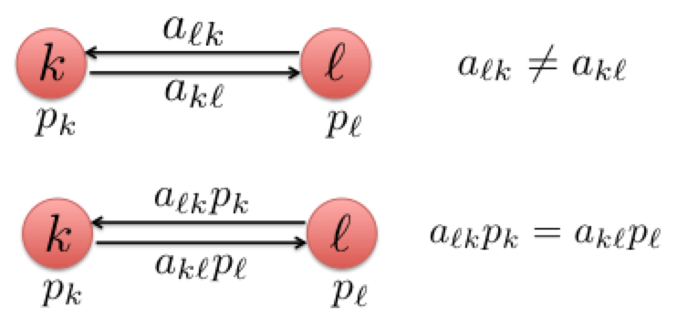
It is worth noting that the local balancing condition (15) is satisfied by several important left-stochastic policies, as illustrated in four examples below. Thus, let for agent . Then condition (11) becomes
| (17) |
where .
Policy 1 (Hastings rule) The first policy we consider is the Hastings rule. Given and , we select as [14, 52]:
| (18) |
where (the number of neighbors of agent ). It can be verified that is left-stochastic, and that the entries of its Perron eigenvector are given by
| (19) |
Let
| (20) |
With (18) and (19), it is easy to verify that
| (21) |
If , it is obvious that (15) holds. If , then . In this case, .
Furthermore, we can also verify that when and are given, are generated through (18), and is chosen as in (20), then condition (11) is satisfied.
Policy 2 (Averaging rule) The second policy we consider is the popular average combination rule where is chosen as
| (22) |
The entries of the Perron eigenvector are given by
| (23) |
With (22) and (23), it clearly holds that
| (24) |
which implies (15).
We can further verify that when is set as
| (25) |
for some positive constant step-size and is set as
| (26) |
then condition (11) will hold.
Policy 3 (Relative-degree rule) The third policy we consider is the relative-degree combination rule [53] where is chosen as
| (27) |
and the entries of the Perron eigenvector are given by
| (28) |
With (27) and (28), it clearly holds that
| (29) |
which implies (15).
Policy 4 (Doubly stochastic policy) If matrix is primitive, symmetric, and doubly stochastic, its Perron eigenvector is . In this situation, the local balance condition (15) holds automatically.
Furthermore, if we assume each agent employs the step-size for some positive constant step-size , it can be verified that condition (11) holds with
| (32) |
There are various rules to generate a primitive, symmetric and doubly stochastic matrix. Some common rules are the Laplacian rule, maximum-degree rule, Metropolis rule and other rules that listed in Table 14.1 in [14].
Policy 5 (Other locally-balanced policies) For other left-stochastic-policies for which closed-form expressions for the Perron entries need not be available, the Perron eigenvector can be learned iteratively to ensure that the step-sizes end up satisfying (13). Before we explain how this can be done, we remark that since the combination matrix is left-stochastic in our formulation, the power iteration employed in push-sum implementations cannot be applied since it works for right-stochastic policies. We proceed instead as follows.
Since is primitive and left-stochastic, it is shown in [54, 14] that
| (33) |
This relation also implies
| (34) |
Now let be the -th column of the identity matrix . Furthermore, let each agent keep an auxiliary variable with each initialized to . We also introduce
| (35) | ||||
| (36) |
By iterating according to
| (37) |
we have
| (38) |
Since , it can be verified that . Substituting into (II-B), we have In summary, it holds that
| (39) |
where is the -th entry of the vector . Therefore, if we set
| (40) |
then it follows that
| (41) |
We finally note that the quantity that appears in the denominator of (40) can be guaranteed non-zero. This can be seen as follows. From the power iteration (37), we have
| (42) |
Since for any and the combination matrix has non-negative entries, we conclude that for . In addition, focusing on the -th entry, we have
| (43) |
where the inequality (*) holds because and . Since , if we let , i.e., each agent assigns positive weight to itself, we have
| (44) |
In other words, the condition can guarantee the positiveness of . This condition is not restrictive because, for example, we can replace the power iteration (42) by
| (45) |
where we are using the coefficients instead of . This is possible because the matrices and are both left-stochastic and have the same Perron vector . Note that no matter whether is zero or not.
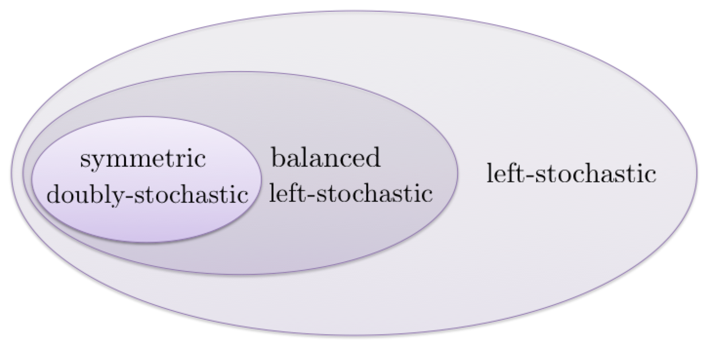
We illustrate in Fig. 2 the relations among the classes of symmetric doubly-stochastic, balanced left-stochastic, and left-stochastic combination matrices. It is seen that every symmetric doubly-stochastic matrix is both left-stochastic and balanced. We indicated earlier that the EXTRA consensus algorithm was derived in [38] with exact convergence properties for symmetric doubly-stochastic matrices. Here, in the sequel, we shall derive an exact diffusion strategy with exact convergence guarantees for the larger class of balanced left-stochastic matrices (which is therefore also applicable to symmetric doubly-stochastic matrices). We will show in Part II[2] that the exact diffusion implementation has a wider stability range than EXTRA consensus; this is a useful property since larger step-sizes can be used to attain larger convergence rates.
Remark 3. (Convergence guarantees) One may wonder whether exact convergence can be guaranteed for the general left-stochastic matrices that are not necessarily balanced (i.e., whether the convergence property can be extended beyond the middle elliptical area in Fig. 2). It turns out that one can provide examples of combination matrices that are left-stochastic (but not necessarily balanced) for which exact convergence occurs and others for which exact convergence does not occur (see, e.g., the examples in Section V and Figs. 8 and 9). In other words, exact convergence is not always guaranteed beyond the balanced class. This conclusion is another useful contribution of this work; it shows that there is a boundary inside the set of left-stochastic matrices within which convergence can be always guaranteed (namely, the set of balanced matrices).
It is worth noting that the recent works [47, 46] extend the consensus-based EXTRA method to the case of directed networks by employing a push-sum technique. These extensions do not require the local balancing condition but they establish convergence only if the step-size parameter falls within an interval where and are two positive constants. However, it is not proved in these works whether this interval is feasible, i.e., whether . In fact, we will construct examples in Section V for which both exact diffusion and push-sum EXTRA will diverge for any step-size . In other words, both exact diffusion and EXTRA methods need not work well for directed networks. This is a disadvantage in comparison with DIGing-based methods [39, 40, 41, 42, 43].
In summary, when locally-balanced policies is employed, exact diffusion is more communication efficient and also more stable than other techniques including DIGing methods and EXTRA. However, just like EXTRA, the exact diffusion strategy is applicable to undirected (rather than directed) graphs.
II-C Useful Properties
We now establish several useful properties for primitive left-stochastic matrices that satisfy the local balance condition (15). These properties will be used in the sequel.
Lemma 1 (Properties of ).
When satisfies the local balance condition (15), it holds that the matrix is primitive, symmetric, and doubly stochastic.
Proof.
With condition (15), the symmetry of is obvious. To check the primitiveness of , we need to verify two facts, namely, that: (a) at least one diagonal entry in is positive, and (b) there exists at least one path with nonzero weights between any two agents. It is easy to verify condition (a) because is already primitive and . For condition (b), since is connected and all diagonal entries of are positive, then if there exists a path with nonzero coefficients linking agents and under , the same path will continue to exist under . Moreover, since all diagonal entries of are positive, then the same path will also exist under . Finally, is doubly stochastic because
| (46) |
| (47) |
Lemma 2 (Nullspace of ).
When satisfies the local balance condition (15), it holds that is symmetric and positive semi-definite. Moreover, it holds that
| (48) |
where denotes the null space of its matrix argument.
Proof.
Let denote the -th largest eigenvalue of . Recall from Lemma 1 that is primitive and doubly stochastic. Therefore, according to Lemma F.4 from [14] it holds that
| (49) |
It follows that the eigenvalues of are non-positive so that .
Note further from (49) that the matrix has a single eigenvalue at one with multiplicity one. Moreover, from (47) we know that the vector is a right-eigenvector associated with this eigenvalue at one. Based on these two facts, we have
| (50) |
for any constant . Relation (50) is equivalent to
| (51) |
which confirms (48).
Corollary 1 (Nullspace of ).
Let and . When satisfies the local balance condition (15), it holds that
| (52) |
Moreover, for any block vector in the nullspace of with entries , it holds that
| (53) |
Proof.
Since has a single eigenvalue at with multiplicity one, we conclude that will have an eigenvalue at with multiplicity . Next we denote the columns of the identity matrix by where . We can verify that is a right-eigenvector associated with the eigenvalue because
| (54) |
Now since any two vectors in the set are mutually independent, we conclude that
| (55) |
These equalities establish (1). From (1) we can also conclude (53) because
| (56) |
from some . The direction “” of (53) is obvious.
Lemma 3 (Real eigenvalues).
When satisfies the local balance condition (15), it holds that is diagonalizable with real eigenvalues in the interval , i.e.,
| (57) |
where , and
| (58) |
Proof.
According to the local balance condition (16), is symmetric. Using the fact that is diagonal, it holds that
| (59) |
which shows that the matrix on the left-hand side is symmetric. Therefore, can be decomposed as
| (60) |
where is an orthogonal matrix and is a real diagonal matrix. From (60), we further have that
| (61) |
If we let , we reach the decomposition (57). Moreover, since is a primitive left-stochastic matrix, according to Lemma F.4 in [14], the eigenvalues of satisfy (58).
For ease of reference, we collect in Table I the properties established in Lemmas 1 through 3 for balanced primitive left-stochastic matrices .
| Properties of balanced primitive left-stochastic matrices |
| is diagonalizable with real eigenvalues in ; |
| has a single eigenvalue at ; |
| is symmetric, primitive, doubly-stochastic; |
| is positive semi-definite; |
| ; |
| . |
III Penalized Formulation of Diffusion
In this section, we employ the properties derived in the previous section to reformulate the unconstrained optimization problem (5) into the equivalent constrained problem (74), which will be solved using a penalized formulation. This derivation will help clarify the origin of the bias from (14) in the standard diffusion implementation.
III-A Constrained Problem Formulation
To begin with, note that the unconstrained problem (5) is equivalent to the following constrained problem:
| (62) |
Now we introduce the block vector and
| (63) |
With (53) and (63), problem (III-A) is equivalent to
| (64) |
From Lemma 2, we know that is symmetric and positive semi-definite. Therefore, we can decompose
| (65) |
where is a non-negative diagonal matrix and is an orthogonal matrix. If we introduce the symmetric square-root matrix
| (66) |
then it holds that
| (67) |
Let so that
| (68) |
Lemma 4 (Nullspace of ).
With defined as in (66), it holds that
| (69) |
Proof.
To prove , it is enough to prove
| (70) |
Indeed, notice that
| (71) |
The reverse direction “” in (70) is obvious.
III-B Penalized Formulation
There are many techniques to solve constrained problems of the form (74). One useful and popular technique is to add a penalty term to the cost function and to consider instead a penalized problem of the form:
| (75) |
where is a penalty parameter. Problem (75) is not equivalent to (74) but is a useful approximation. The smaller the value of is, the closer the solutions of problems (74) and (75) become to each other [55, 56, 57]. We now verify that the diffusion strategy (6)–(7) follows from applying an incremental technique to solving the approximate penalized problem (75), not the real problem (74). It will then become clear that the diffusion estimate cannot converge to the exact solution of problem (5) (or (74)).
Since (68) holds, problem (75) is equivalent to
| (76) |
This is an unconstrained problem, which we can solve using, for example, a diagonally-weighted incremental algorithm, namely,
| (77) |
The above recursion can be simplified as follows. Assume we select
| (78) |
where is the same constant used in relation (11). Recall from (20), (26), (31) and (32) that and hence . Moreover, from the definition of in (63), we have
| (82) |
Using (11), namely,
| (83) |
we find that
| (87) |
We further introduce the aggregate cost (which is similar to (63) but without the weighting coefficients):
| (88) |
and note that
| (92) |
Let . Using (87) and (92), the first recursion in (77) can be rewritten as
| (93) |
For the second recursion of (77), it can be rewritten as
| (94) |
because . Relations (93)–(94) are equivalent to (6)–(7). Specifically, if we collect all iterates from across all agents into block vectors , then (6)–(7) would lead to (93)–(94). From this derivation, we conclude that the diffusion algorithm (6)–(7) can be interpreted as performing the diagonally-weighted incremental construction (77) to solve the approximate penalized problem (76). Since this construction is not solving the real problem (5), there exists a bias between its fixed point and the real solution . As shown in (14), the size of this bias is related to . When is small, the bias is also small. This same conclusion can be seen by noting that a small corresponds to a large penalty factor under which the solutions to problems (5) and (74) approach each other.
IV Development of Exact Diffusion
We now explain how to adjust the diffusion strategy (6)–(7) to ensure exact convergence to . Instead of solving the approximate penalized problem (76), we apply the primal-dual saddle point method to solve the original problem (74) directly. We continue to assume that the combination policy is primitive and satisfies the local balancing condition (15).
To solve (74) with saddle point algorithm, we first introduce the augmented Lagrangian function:
| (95) |
where is the dual variable. The standard primal-dual saddle point algorithm has recursions
| (96) |
The first recursion in (96) is the primal descent while the second recursion is the dual ascent. Now, instead of performing the descent step directly as shown in the first recursion in (96), we perform it in an incremental manner. Thus, let
| (97) |
so that
| (98) |
The diagonally incremental recursion that corresponds to the first step in (96) is then:
| (99) |
where in the second recursion of (99) we introduced
| (100) |
We know from (58) that the eigenvalues of are positive and lie within the interval . In (99), if we substitute the first and second recursions into the third one, and also recall (87) that , then we get
| (101) |
Replacing the first recursion in (96) with (101), the previous primal-dual saddle point recursion (96) becomes
| (102) |
Recursion (102) is the primal-dual form of the exact diffusion recursion we are seeking. For the initialization, we set and to be any value, and hence for we have
| (103) |
We can rewrite (102) in a simpler form by eliminating the dual variable from the first recursion. For from (102) we have
| (104) |
From the second step in (102) we have
| (105) |
Substituting (IV) into (104), we arrive at
| (106) |
Recursion (106) is the primal version of the exact diffusion.
We can rewrite (106) in a distributed form that resembles (6)–(7) more closely, as listed below in Algorithm 1, where we denote the entries of by . It is observed in Algorithm 1 that the exact diffusion strategy resembles (6)–(7) to great extent, with the addition of a “correction” step between the adaptation and combination step. In the correction step, the intermediate estimate is “corrected” by removing from it the difference between and from the previous iteration. Moreover, it is also observed that the exact and standard diffusion strategies have essentially the same computational complexity, apart from ( is the dimension of ) additional additions per agent in the correction step of the exact implementation. Also, there is one combination step in each iteration, which reduces the communication cost by about one half in comparison to recent DIGing-based works [39, 40, 41, 42, 43].
Algorithm 1 (Exact diffusion strategy for agent )
Setting:
Let , and arbitrary. Set .
Setting:
Let .
Repeat for
| (107) | ||||
| (108) | ||||
| (109) |
One can directly run Algorithm 1 when the Perron entries are known beforehand, as explained in Section II-B. When this is not the case, we can blend iteration (37) into the algorithm and modify it as follows.
Algorithm 1’ (Exact diffusion strategy when is unknown)
Setting:
Let , and arbitrary. Set ,
and .
Repeat for
| (110) | ||||
| (111) | ||||
| (112) | ||||
| (113) |
V Significance of Balanced Policies
The stability and convergence properties of the exact diffusion strategy (107)–(109) will be examined in detail in Part II [2]. There we will show that exact diffusion is guaranteed to converge for all balanced left-stochastic matrices for sufficiently small step-sizes. The local balancing property turns out to be critical in the sense that convergence may or may not occur if we move beyond the set of balanced policies. We can illustrate these possibilities here by means of examples. The two examples discussed in the sequel highlight the importance of having balanced combination policies for exact convergence.
Thus, consider the primal recursion of the exact diffusion algorithm (106), where is a general left-stochastic matrix. We subtract from both sides of (106), to get the error recursion
| (114) |
where . When is twice-differentiable, we can appeal to the mean-value theorem from Lemma D.1 in [14], which allows us to express each difference
| (115) |
If we let
| (116) |
and introduce the block diagonal matrix:
| (117) |
then we can rewrite
| (118) |
Notice that
| (119) |
Combining (114), (V) and the fact , we have
| (124) |
where
| (127) | ||||
| (130) |
In the next two examples, we consider the simple case where the dimension , for , and the step-size = , where
| (131) |
In this situation, the matrix reduces to
| (134) |
Moreover, we also assume is iteration independent, i.e.,
| (135) |
This assumption holds for quadratic costs . Under the above conditions, we have
| (142) |
which implies that is one eigenvalue of no matter what the step-size is. However, since is initialized as and, hence, lies in , the eigenvalue will not influence the convergence of recursion (124) (the detailed explanation is spelled out in Sections II and III of Part II[2]). Let denote the remaining eigenvalues of , and introduce
| (143) |
It is that determines the convergence of recursion (124): the exact diffusion recursion (124) will diverge if , and will converge if .
Example 1 (Diverging case). Consider the following left-stochastic matrix :
| (148) |
It can be verified that is primitive, left-stochastic but not balanced. For such , its Perron eigenvector can be calculated in advance, and hence is also known. Also, is assumed to satisfy
| (149) |
Substituting the above and into shown in (134), it can be verified that
| (150) |
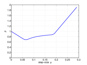
for any step-size . The proof is given in Appendix A by appealing to the Jury test for stability. In the top plot in Fig. 8, we show the spectral radius for step-sizes . It is observed that .
By following similar arguments, we can find a counter example such that EXTRA will also diverge for any step-size , even if we assume the Perron eigenvector is known in advance. For example, if
| (156) |
and
| (157) |
one can verify that EXTRA will diverge for any by following the arguments in Appendix A. As a result, the push-sum based algorithms [47, 46] that extend EXTRA to non-symmetric networks cannot always converge. This example indicates that the stability range provided in [47, 46] may not always be feasible.
Example 2 (Converging case). Consider the following left-stochastic matrix :
| (163) |
It can be verified that is primitive and not balanced. Also, is assumed to satisfy
| (164) |
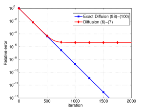
Substituting the above and into (134), it can be verified that . Therefore, when is sufficiently small, will dominate in and . The simulations in Fig. 9 confirm this fact. In particular, it is observed that when . As a result, the exact diffusion will converge when under this setting.
VI Numerical Experiments
In this section we illustrate the performance of the proposed exact diffusion algorithm. In all figures, the -axis indicates the relative error, i.e., , where and .
VI-A Distributed Least-squares
In this experiment, we focus on solving the least-squares problem over the network shown in 3:
| (165) |
where the network size and the dimension . Each entry in both and is generated from the standard Gaussian distribution .
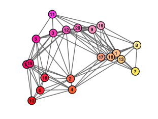
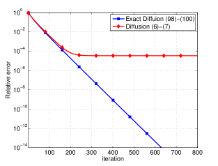
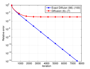
We compare the convergence behavior of standard diffusion and the exact diffusion algorithm in the simulation. The left-stochastic matrix is generated through the averaging rule (see (22)), and each agent employs step-size (see (25)) where is a small constant step-size. The convergence of both algorithms is shown in Fig. 4, where we set . It is observed that the standard diffusion algorithm converges to a neighborhood of on the order , while the exact diffusion converges exponentially fast to the exact solution . This figure confirms that exact diffusion corrects the bias in standard diffusion.
VI-B Distributed Logistic Regression
We next consider a pattern classification scenario. Each agent holds local data samples , where is a feature vector and is the corresponding label. Moreover, the value is the number of local samples at each agent. All agents will cooperatively solve the regularized logistic regression problem over the network in Fig. 3:
| (166) |
In the experiments, we set , , and . For local data samples at agent , each is generated from the standard normal distribution . To generate , we first generate an auxiliary random vector with each entry following . Next, we generate from a uniform distribution . If then is set as ; otherwise is set as . We set .
We still compare the convergence behavior of the standard diffusion and exact diffusion. The left-stochastic matrix is generated through the averaging rule, and each agent employs step-size . The convergence of both algorithms is shown in Fig. 5. The step-size . It is also observed that the exact diffusion corrects the bias in standard diffusion.
VI-C Averaging Rule v.s. Doubly Stochastic Rules
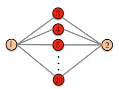
In this subsection we test the convergence performance of exact diffusion under different combination matrices. Consider a network with a highly unbalanced topology as shown in Fig. 6. Nodes and are “celebrities” with many neighbors, while the other nodes just have two neighbors each. Such a network topology is quite common over social networks.
Interestingly, both the maximum degree rule and the Metropolis rule will generate the same doubly-stochastic combination matrix for this network. Let be the Laplacian matrix associated with that network, then the generated doubly-stochastic combination matrix is
| (167) |
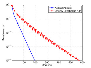
This combination matrix merges information just slightly better than the identity matrix because the term is quite small, which is not efficient. In contrast, the normal agent (where ) will assign to incoming information from agents and if the averaging rule is used, which combines information more efficiently and hence leads to faster convergence. In Fig. 7, we compare these two combination matrices over the distributed least-square problem (165). The step-sizes are carefully chosen such that each combination matrix reaches its fastest convergence. As expected, it is observed that the averaging rule is almost three times faster than the doubly-stochastic rule.
VI-D Exact Diffusion for General Left-Stochastic
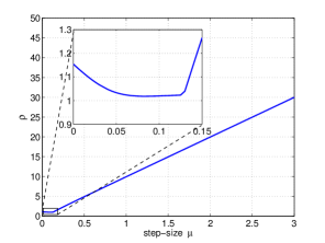
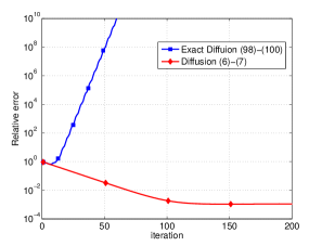
In this subsection we test exact diffusion for the general left-stochastic shown in Section V. In Fig. 8 we test the setting of Example in which is in the form of (148) and is (149). We introduce . In the top plot, we illustrate how varies with step-size . In this plot, the step-size varies over , and the interval between two consecutive is . It is observed that for any , which confirms with our conclusion that exact diffusion will diverge for any step-size under the setting in Example . In the bottom plot of Fig. 8 we illustrate the standard diffusion converges to a neighborhood of on the order of for , while the exact diffusion diverges.
In Fig. 9 we test the setting of Example in which is in the form of (163) and is of (164). In the top plot, we illustrate how varies with . It is observed that when , which implies that the exact diffusion recursion (124) will converge when . In the bottom figure, with it is observed that exact diffusion will converge exactly to . Figures. 8 and 9 confirm that general left-stochastic cannot always guarantee convergence to .
VII CONCLUDING REMARKS
This work developed a diffusion optimization
strategy with guaranteed exact convergence for a broad
class of combination policies. The strategy is applicable to non-symmetric
left-stochastic combination matrices, while many earlier
developments on exact consensus implementations are
limited to doubly-stochastic matrices or right-stochastic matrices; these latter matrices
impose stringent constraints on the network topology. Part II[2] of this work establishes analytically, and by means of examples and simulations, the superior convergence and stability properties of exact diffusion implementations.
Appendix A Proof of (150)
The characteristic polynomial of is given by
| (168) |
and
| (169) |
| (170) |
It is easy to observe from (168) that is one eigenvalue of . As mentioned in (142) and its following paragraph, this eigenvalue does not influence the convergence of recursion (124) because of the initial conditions. It is the roots of that decide the convergence of the exact diffusion recursion (124). Now we will prove that there always exists some root that stays outside the unit-circle no matter what the step-size is. In other words, is not stable for any .
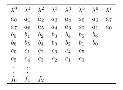
Since is a -th order polynomial, its roots are not easy to calculate directly. Instead, we apply the Jury stability criterion [58] to decide whether has roots outside the unit-circle. First we construct the Jury table as shown in Fig. 10, where
| (173) | ||||
| (176) | ||||
| (179) | ||||
According to the Jury stability criterion, is stable (i.e., all roots of are within the unit-circle) if, and only if, the following conditions hold:
| (180) |
If any one of the above conditions is violated, is not stable. Next we check each of the conditions:
(1) is satisfied for any since
| (181) |
(2) . To guarantee this condition, we need to require that
| (182) |
With the help of Matlab, we can verify that
| (183) |
(3) . To guarantee this condition, we need
| (184) |
which is equivalent to requiring
| (185) |
With (181), (183) and (185), we conclude that when
| (186) |
conditions (1), (2) and (3) will be satisfied simultaneously. Moreover, with the help of Matlab, we can also verify that the step-size range (186) will also meet conditions (4) , (5) and (6) . Now we check the last two conditions.
(7) . To guarantee this condition, the step-size is required to satisfy
| (187) |
(8) . To guarantee this condition, the step-size is required to satisfy
| (188) |
Comparing (186), (187) and (188), it is observed that the intersection of these three ranges is empty, which implies that there does not exist a value for that makes all conditions (1)–(8) hold. Therefore, we conclude that is not stable for any step-size .
References
- [1] K. Yuan, B. Ying, X. Zhao, and A. H. Sayed, “Exact diffusion strategy for optimization by networked agents,” in Proc. EUSIPCO, Kos island, Greece, Sep. 2017, 5 pages.
- [2] K. Yuan, B. Ying, X. Zhao, and A. H. Sayed, “Exact dffusion for distributed optimization and learning – Part II: Convergence analysis,” Submitted for publication, Also available as arXiv:1702.05142, Feb. 2017.
- [3] D. Estrin, L. Girod, G. Pottie, and M. Srivastava, “Instrumenting the world with wireless sensor networks,” in Proc. IEEE International Conference on Acoustics, Speech, and Signal Processing (ICASSP), Salt Lake City, UT, 2001, vol. 4, pp. 2033–2036.
- [4] L. A. Rossi, B. Krishnamachari, and C. C.J. Kuo, “Distributed parameter estimation for monitoring diffusion phenomena using physical models,” in Proc. IEEE Conference on Sensor and Ad Hoc Communications and Networks (SECON), Santa Clara, CA, 2004, pp. 460–469.
- [5] D. Li, K. D. Wong, Y. Hu, and A. M. Sayeed, “Detection, classification, and tracking of targets,” IEEE Signal Processing Magazine, vol. 19, no. 2, pp. 17–29, 2002.
- [6] I. F. Akyildiz, W. Su, Y. Sankarasubramaniam, and E. Cayirci, “A survey on sensor networks,” IEEE Communications Magazine, vol. 40, no. 8, pp. 102–114, 2002.
- [7] W. Ren, R. W. Beard, and E. M. Atkins, “Information consensus in multivehicle cooperative control,” IEEE Control Systems Magazine, vol. 27, no. 2, pp. 71–82, 2007.
- [8] K. Zhou and S. I. Roumeliotis, “Multirobot active target tracking with combinations of relative observations,” IEEE Transactions on Robotics, vol. 27, no. 4, pp. 678–695, 2011.
- [9] S. M. Amin and B. F. Wollenberg, “Toward a smart grid: power delivery for the 21st century,” IEEE Power and Energy Magazine, vol. 3, no. 5, pp. 34–41, 2005.
- [10] C. Ibars, M. Navarro, and L. Giupponi, “Distributed demand management in smart grid with a congestion game,” in Proc. IEEE International Conference on Smart Grid Communications (SmartGridComm),, Gaithersburg, MD, 2010, IEEE, pp. 495–500.
- [11] H. Kim, Y.-J. Kim, K. Yang, and M. Thottan, “Cloud-based demand response for smart grid: Architecture and distributed algorithms,” in Proc. IEEE International Conference on Smart Grid Communications (SmartGridComm), Brussels, Belgium, 2011, IEEE, pp. 398–403.
- [12] G. B. Giannakis, V. Kekatos, N. Gatsis, S.-J. Kim, H. Zhu, and B W., “Monitoring and optimization for power grids: A signal processing perspective,” IEEE Signal Processing Magazine, vol. 30, no. 5, pp. 107–128, 2013.
- [13] A. H. Sayed, “Adaptive networks,” Proceedings of the IEEE, vol. 102, no. 4, pp. 460–497, April 2014.
- [14] A. H. Sayed, “Adaptation, learning, and optimization over networks,” Foundations and Trends in Machine Learning, vol. 7, no. 4-5, pp. 311–801, 2014.
- [15] J. Chen and A. H. Sayed, “Diffusion adaptation strategies for distributed optimization and learning over networks,” IEEE Transactions on Signal Processing, vol. 60, no. 8, pp. 4289–4305, 2012.
- [16] J. Chen and A. H. Sayed, “On the learning behavior of adaptive networks—Part I: Transient analysis,” IEEE Transactions on Information Theory, vol. 61, no. 6, pp. 3487–3517, 2015.
- [17] J. Chen and A. H. Sayed, “On the learning behavior of adaptive networks—Part II: Performance analysis,” IEEE Transactions on Information Theory, vol. 61, no. 6, pp. 3518–3548, 2015.
- [18] J. C. Duchi, A. Agarwal, and M. J. Wainwright, “Dual averaging for distributed optimization: convergence analysis and network scaling,” IEEE Transactions on Automatic Control, vol. 57, no. 3, pp. 592–606, 2012.
- [19] J. Chen, Z. J. Towfic, and A. H. Sayed, “Dictionary learning over distributed models,” IEEE Transactions on Signal Processing, vol. 63, no. 4, pp. 1001–1016, 2015.
- [20] S. Chouvardas, K. Slavakis, Y. Kopsinis, and S. Theodoridis, “A sparsity promoting adaptive algorithm for distributed learning,” IEEE Transactions on Signal Processing, vol. 60, no. 10, pp. 5412–5425, Oct. 2012.
- [21] X. Zhao and A. H. Sayed, “Distributed clustering and learning over networks,” IEEE Transactions on Signal Processing, vol. 63, no. 13, pp. 3285–3300, 2015.
- [22] J. Chen, C. Richard, and A. H. Sayed, “Diffusion LMS over multitask networks,” IEEE Transactions on Signal Processing, vol. 63, no. 11, pp. 2733–2748, 2015.
- [23] A. Nedić and A. Ozdaglar, “Distributed subgradient methods for multi-agent optimization,” IEEE Transactions on Automatic Control, vol. 54, no. 1, pp. 48–61, 2009.
- [24] A. G. Dimakis, S. Kar, J. M. F. Moura, M. G. Rabbat, and A. Scaglione, “Gossip algorithms for distributed signal processing,” Proceedings of the IEEE, vol. 98, no. 11, pp. 1847–1864, 2010.
- [25] S. Kar and J. M. F. Moura, “Convergence rate analysis of distributed gossip (linear parameter) estimation: Fundamental limits and tradeoffs,” IEEE Journal of Selected Topics in Signal Processing, vol. 5, no. 4, pp. 674–690, 2011.
- [26] S. Kar, J. M. F. Moura, and K. Ramanan, “Distributed parameter estimation in sensor networks: Nonlinear observation models and imperfect communication,” IEEE Transactions on Information Theory, vol. 58, no. 6, pp. 3575–3605, 2012.
- [27] K. Yuan, Q. Ling, and W. Yin, “On the convergence of decentralized gradient descent,” SIAM Journal on Optimization, vol. 26, no. 3, pp. 1835–1854, 2016.
- [28] R. Olfati-Saber and J. S. Shamma, “Consensus filters for sensor networks and distributed sensor fusion,” in Proc. IEEE Conference on Decision and Control (CDC). IEEE, 2005, pp. 6698–6703.
- [29] S. Sardellitti, M. Giona, and S. Barbarossa, “Fast distributed average consensus algorithms based on advection-diffusion processes,” IEEE Transactions on Signal Processing, vol. 58, no. 2, pp. 826–842, 2010.
- [30] P. Braca, S. Marano, and V. Matta, “Running consensus in wireless sensor networks,” in Proc. IEEE International Conference on Information Fusion, Cologne, Germany, 2008, pp. 1–6.
- [31] J. Chen and A. H. Sayed, “Distributed pareto optimization via diffusion strategies,” IEEE Journal of Selected Topics in Signal Processing, vol. 7, no. 2, pp. 205–220, 2013.
- [32] G. Mateos, J. A. Bazerque, and G. B. Giannakis, “Distributed sparse linear regression,” IEEE Transactions on Signal Processing, vol. 58, no. 10, pp. 5262–5276, 2010.
- [33] J. F. Mota, J. M. Xavier, P. M. Aguiar, and M. Püschel, “D-ADMM: A communication-efficient distributed algorithm for separable optimization,” IEEE Transactions on Signal Processing, vol. 61, no. 10, pp. 2718–2723, 2013.
- [34] W. Shi, Q. Ling, K. Yuan, G. Wu, and W. Yin, “On the linear convergence of the ADMM in decentralized consensus optimization,” IEEE Transactions on Signal Processing, vol. 62, no. 7, pp. 1750–1761, 2014.
- [35] Q. Ling, W. Shi, G. Wu, and A. Ribeiro, “DLM: Decentralized linearized alternating direction method of multipliers,” IEEE Transactions on Signal Processing, vol. 63, no. 15, pp. 4051–4064, 2015.
- [36] T.-H. Chang, M. Hong, and X. Wang, “Multi-agent distributed optimization via inexact consensus ADMM,” IEEE Transactions on Signal Processing, vol. 63, no. 2, pp. 482–497, 2015.
- [37] A. Mokhtari, W. Shi, Q. Ling, and A. Ribeiro, “DQM: Decentralized quadratically approximated alternating direction method of multipliers,” IEEE Transactions on Signal Processing,, vol. 64, no. 19, pp. 5158–5173, 2016.
- [38] W. Shi, Q. Ling, G. Wu, and W. Yin, “EXTRA: An exact first-order algorithm for decentralized consensus optimization,” SIAM Journal on Optimization, vol. 25, no. 2, pp. 944–966, 2015.
- [39] P. D. Lorenzo and G. Scutari, “NEXT: In-network nonconvex optimization,” IEEE Transactions on Signal and Information Processing over Networks, vol. 2, no. 2, pp. 120–136, 2016.
- [40] A. Nedić, A. Olshevsky, and W. Shi, “Achieving geometric convergence for distributed optimization over time-varying graphs,” arXiv:1607.03218, Jul. 2016.
- [41] G. Qu and N. Li, “Harnessing smoothness to accelerate distributed optimization,” to appear in IEEE Transactions on Control of Network Systems, 2017.
- [42] J. Xu, S. Zhu, Y. C. Soh, and L. Xie, “Augmented distributed gradient methods for multi-agent optimization under uncoordinated constant stepsizes,” in IEEE Conference on Decision and Control (CDC), Osaka, Japan, 2015, pp. 2055–2060.
- [43] A. Nedić, A. Olshevsky, W. Shi, and C. A. Uribe, “Geometrically convergent distributed optimization with uncoordinated step-sizes,” arXiv:1609.05877, Sep. 2016.
- [44] K.I. Tsianos, S. Lawlor, and M. G. Rabbat, “Push-sum distributed dual averaging for convex optimization,” in IEEE Conference on Decision and Control (CDC), Maui, Hawaii, 2012, pp. 5453–5458.
- [45] A. Nedić and A. Olshevsky, “Stochastic gradient-push for strongly convex functions on time-varying directed graphs,” IEEE Transactions on Automatic Control, vol. 61, no. 12, pp. 3936–3947, 2016.
- [46] C. Xi and U. A. Khan, “On the linear convergence of distributed optimization over directed graphs,” arXiv:1510.02149, Oct. 2015.
- [47] J. Zeng and W. Yin, “ExtraPush for convex smooth decentralized optimization over directed networks,” arXiv:1511.02942, Nov. 2015.
- [48] S. U. Pillai, T. Suel, and S. Cha, “The Perron-Frobenius theorem: some of its applications,” IEEE Signal Processing Magazine, vol. 22, no. 2, pp. 62–75, 2005.
- [49] X. Zhao, Learning under Imperfections by Networked Agents, Ph.D. Dissertation, Electrical Engineering Department, UCLA, Sep. 2014.
- [50] P. Whittle, “Equilibrium distributions for an open migration process,” Journal of Applied Probability, pp. 567–571, 1968.
- [51] J. R. Norris, Markov Chains, Number 2. Cambridge university press, 1998.
- [52] W. K. Hastings, “Monte carlo sampling methods using Markov chains and their applications,” Biometrika, vol. 57, no. 1, pp. 97–109, 1970.
- [53] F. S. Cattivelli and A. H. Sayed, “Diffusion strategies for distributed Kalman filtering and smoothing,” IEEE Transactions on automatic control, vol. 55, no. 9, pp. 2069–2084, 2010.
- [54] A. Nedic and A. Olshevsky, “Distributed optimization over time-varying directed graphs,” IEEE Transactions on Automatic Control, vol. 60, no. 3, pp. 601–615, 2015.
- [55] S. Boyd and L. Vandenberghe, Convex Optimization, Cambridge university press, 2004.
- [56] R. Fletcher, Practical Methods of Optimization,, John Wiley & Sons, New York, NY, USA, second edition, 1987.
- [57] Z. J. Towfic and A. H. Sayed, “Adaptive penalty-based distributed stochastic convex optimization,” IEEE Transactions on Signal Processing, vol. 62, no. 15, pp. 3924–3938, 2014.
- [58] E. I. Jury, “A simplified stability criterion for linear discrete systems,” Proceedings of the IRE, vol. 50, no. 6, pp. 1493–1500, 1962.