Grassmannian flows and applications to nonlinear partial differential equations

Abstract

We show how solutions to a large class of partial differential equations with nonlocal Riccati-type nonlinearities can be generated from the corresponding linearized equations, from arbitrary initial data. It is well known that evolutionary matrix Riccati equations can be generated by projecting linear evolutionary flows on a Stiefel manifold onto a coordinate chart of the underlying Grassmann manifold. Our method relies on extending this idea to the infinite dimensional case. The key is an integral equation analogous to the Marchenko equation in integrable systems, that represents the coodinate chart map. We show explicitly how to generate such solutions to scalar partial differential equations of arbitrary order with nonlocal quadratic nonlinearities using our approach. We provide numerical simulations that demonstrate the generation of solutions to Fisher–Kolmogorov–Petrovskii–Piskunov equations with nonlocal nonlinearities. We also indicate how the method might extend to more general classes of nonlinear partial differential systems.

1 Introduction

It is well known that solutions to many integrable nonlinear partial differential equations can be generated from solutions to a linear integrable equation namely the Gel’fand–Levitan–Marchenko equation. It is an example of a generic dressing transformation which we shall express in the form

$$g(x,y)=p(x,y)-\int_{x}^{\infty}g(x,z)q^{\prime}(z,y;x)\,\mathrm{d}z,$$ (1)

for $y\geqslant x$. See Zakharov and Shabat ZS or Dodd, Eilbeck, Gibbon and Morris DEGM for more details. Here all the functions shown may depend explicitly on time $t$, and we suppose that $q^{\prime}$ and $p$ represent given data and $g$ is the solution. Typically $p$ represents the scattering data and takes the form $p=p(x+y)$ while $q^{\prime}$ depends on $p$, for example $q^{\prime}=-p$ in the case of the Korteweg de Vries equation. See Ablowitz, Ramani and Segur ARSII for more details. Typically given a nonlinear integrable partial differential equation, the function $p$ is the solution to an associated linear system and the solution to the nonlinear integrable equation is given by $u=-2(\mathrm{d}/\mathrm{d}x)g(x,x)$. See for example Drazin and Johnson (DJ, , p. 86) for the case of the Korteweg de Vries equation. The notion that the solution to a corresponding linear partial differential equation can be used to generate solutions to nonlinear integrable partial differential equations is addressed in the review by Miura Miura . An explicit formula was provided by Dyson Dyson who showed that for the Korteweg de Vries equation the solution to the Gel’fand–Levitan–Marchenko equation along the diagonal $g=g(x,x)$ can be expressed in terms of the derivative of the logarithm of a tau-function or Fredholm determinant. In a series of papers Pöppe P-SG ; P-KdV ; P-KP , Pöppe and Sattinger PS-KP , Bauhardt and Pöppe BP-ZS , and Tracy and Widom TW expressed the solutions to further nonlinear integrable partial differential equations in terms of Fredholm determinants. Importantly Pöppe P-SG explicitly states the idea that:

“For every soliton equation, there exists a linear PDE (called a base equation) such that a map can be defined mapping a solution $p$ of the base equation to a solution $u$ of the soliton equation. The properties of the soliton equation may be deduced from the corresponding properties of the base equation which in turn are quite simple due to linearity. The map $p\to u$ essentially consists of constructing a set of linear integral operators using $p$ and computing their Fredholm determinants.”

From our perspective, the solution $g$ to the dressing transformation represents an element of a Fredholm Grassmann manifold, expressed in a given coordinate patch. Let us briefly explain this perspective here. This will also help motivate the structures we introduce herein. Our original interest in Grassmann manifolds arose in spectral problems associated with $n$th order linear operators on the real line which can be expressed in the form

$${\partial}_{t}{\mathfrak{q}} =A{\mathfrak{q}}+B{\mathfrak{p}}$$ (2a)

$${\partial}_{t}{\mathfrak{p}} =C{\mathfrak{q}}+D{\mathfrak{p}},$$ (2b)

where ${\mathfrak{q}}={\mathfrak{q}}(t)\in{\mathbb{C}}^{k}$ and ${\mathfrak{p}}={\mathfrak{p}}(t)\in{\mathbb{C}}^{n-k}$, with natural numbers $1\leqslant k<n$. In these equations $A=A(t)\in{\mathbb{C}}^{k\times k}$, $B=B(t)\in{\mathbb{C}}^{k\times(n-k)}$, $C=C(t)\in{\mathbb{C}}^{(n-k)\times k}$ and $D=D(t)\in{\mathbb{C}}^{(n-k)\times(n-k)}$ are linear matrix operators. We assume as given that the matrix consisting of the blocks $A$, $B$, $C$ and $D$ has rank $n$ for all $t\in{\mathbb{R}}$. For example, in the case of elliptical eigenvalue problems, we have $(n-k)=k$ and $A=O$, $B=I_{k}$ and $C$ contains the potential function. Then, with $t\in{\mathbb{R}}$ representing a spatial coordinate, the equations above are the corresponding first order representation of such an eigenvalue problem and the first equation corresponds to simply setting the variable ${\mathfrak{p}}$ to be the spatial derivative of ${\mathfrak{q}}$. The goal is to solve such eigenvalue problems by shooting. In such an approach the far-field boundary conditions, let’s focus on the left far-field for the moment, naturally determine a subspace of solutions which decay to zero exponentially fast, though in general at different exponential rates. The choice of $k$ above hitherto was arbitrary, now we retrospectively choose it to be the dimension of this subspace of solutions decaying exponentially in the left far-field. We emphasize it is the data, in this case the far-field data, that determines the dimension $k$ of the subspace we consider. In principle we can integrate $k$ solutions from the left far-field forward in $t$ thus generating a continuous set of $k$-frames evolving with $t\in{\mathbb{R}}$. If $({\mathfrak{q}}_{1},{\mathfrak{p}}_{1})^{\mathrm{\tiny T}},\ldots,({\mathfrak{q}}_{k},{\mathfrak{p}}_{k})^{\mathrm{\tiny T}}$ represent the solutions to the linear system (2) above that make up the components of the $k$-frame, we can represent them by

$$\begin{pmatrix}Q\\ P\end{pmatrix}\coloneqq\begin{pmatrix}{\mathfrak{q}}_{1}&\cdots&{\mathfrak{q}}_{k}\\ {\mathfrak{p}}_{1}&\cdots&{\mathfrak{p}}_{k}\end{pmatrix},$$

where $Q\in{\mathbb{C}}^{k\times k}$ and $P\in{\mathbb{C}}^{(n-k)\times k}$. From the linear system (2) for ${\mathfrak{q}}$ and ${\mathfrak{p}}$ above, the matrices $Q=Q(t)$ and $P=P(t)$ naturally satisfy the linear matrix system

$${\partial}_{t}Q =AQ+BP$$ (3a)

$${\partial}_{t}P =CQ+DP.$$ (3b)

To determine eigenvalues, by matching with the right far-field boundary conditions, the minimal information required is that for the subspace only and not the complete frame information. The Grassmann manifold ${\mathrm{Gr}}({\mathbb{C}}^{n},{\mathbb{C}}^{k})$ is the set of $k$-dimensional subpsaces in ${\mathbb{C}}^{n}$. It is thus the natural context for the subspace evolution and then matching. See Alexander, Gardner and Jones AGJ90 for a comprehensive account; they used the Plücker coordinate representation for the Grassmannian ${\mathrm{Gr}}({\mathbb{C}}^{n},{\mathbb{C}}^{k})$. In Ledoux, Malham and Thümmler LMT , Ledoux, Malham, Niesen and Thümmler LMNT and Beck and Malham BM we chose instead to directly project onto a coordinate patch of the Grassmannian ${\mathrm{Gr}}({\mathbb{C}}^{n},{\mathbb{C}}^{k})$. Assuming that the matrix $Q\in{\mathbb{C}}^{k\times k}$ has rank $k$, we can achieve this as follows. We consider the transformation of coordinates here given by $Q^{-1}$ that renders the first $k<n$ coordinates as orthonormal thus generating the matrix

$$\begin{pmatrix}I_{k}\\ G\end{pmatrix},$$

where $G(t)=P(t)\,Q^{-1}(t)$ for all $t\in{\mathbb{R}}$. Note this includes the data, i.e. $G(-\infty)=P(-\infty)Q^{-1}(-\infty)$. The key point which underlies the ideas in this paper is that $G=G(t)\in{\mathbb{C}}^{(n-k)\times k}$ evolves according to the evolutionary Riccati equation

$${\partial}_{t}G=C+DG-G\,(A+BG),$$ (4)

where $A$, $B$, $C$ and $D$ are the block matrices from the linear evolutionary system (2) above. This equation for $G$ is straightforwardly derived by direct computation. The Grassmannian ${\mathrm{Gr}}({\mathbb{C}}^{n},{\mathbb{C}}^{k})$ is a homogeneous manifold. As such there are many numerical advantages to integrating along it, here this corresponds to computing $G=G(t)$. For instance, the aforementioned differing far-field exponential growth rates are projected out and $G$ provides a useful succinct paramaterization of the subspace. It provides the natural extension of shooting methods to higher order linear spectral problems on the real line; also see Deng and Jones DJ-M . Let us call the procedure of deriving the Riccati equation (4) from the linear equations (3) the forward problem.

However in this finite dimensional context let us now turn this question around. Suppose our goal now is to solve the quadratically nonlinear evolution equation (4) above for some given data $G(-\infty)=G_{0}$. We assume of course the block matrices $A$, $B$, $C$ and $D$ have the properties described above. Let us call this the inverse problem. With the forward problem described above in mind, given such a nonlinear evolution equation to solve, we might naturally assume the nonlinear evolution equation (4) resulted from the projection of a linear Stiefel manifold flow onto a coordinate patch of the underlying Grassmann manifold. From this perspective, since all we are given is $G$ or indeed just the data $G_{0}$, we can naturally assume $G_{0}$ was the result of such a Stiefel to Grassmann manifold projection. In particular we are free to assume that the transformation $Q$ underlying the projection had rank $k$, and indeed $Q(-\infty)$, was simply $I_{k}$ itself. Thus if we suppose we were given data $Q(-\infty)=I_{k}$ and $P(-\infty)=G_{0}$ and that $Q\in{\mathbb{C}}^{k\times k}$ and $P\in{\mathbb{C}}^{(n-k)\times k}$ satisfied the linear evolutionary equations (3) above then indeed $G=PQ^{-1}$ would solve the nonlinear evolution equation (4) above. Note that in this process there is nothing special about the data being prescribed at $t=-\infty$, it could be prescribed at any finite value of $t$, for example $t=0$. In summary, suppose we want to solve the nonlinear Riccati equation (4) for some given data $G(0)=G_{0}\in{\mathbb{C}}^{(n-k)\times k}$. Then if we suppose the matrices $Q\in{\mathbb{C}}^{k\times k}$ and $P\in{\mathbb{C}}^{(n-k)\times k}$ satisfy the linear system of equations (3) with $Q(0)=I_{k}$ and $P(0)=G_{0}$, then the solution $G\in{\mathbb{C}}^{(n-k)\times k}$ to the linear relation $P=G\,Q$ solves the Riccati equation (4) on some possibly small but non-zero interval of existence.

Our goal herein is to extend the idea just outlined to the infinite dimensional setting. Hereafter we always think of $t\in[0,\infty)$ as an evolutionary time variable. The natural extension of the finite rank (matrix) operator setting above to the infinite dimensional case is to pass over to the corresponding setting with compact operators. Thus formally, now suppose $Q=Q(t)$ and $P=P(t)$ are linear operators satisfying the linear system of evolution equations (3) for $t\geqslant 0$. We assume that $A$ and $C$ are bounded operators, while the operators $B$ and $D$ may be bounded or unbounded. We suppose the solution operators $Q=Q(t)$ and $P=P(t)$ are such that for some $T>0$, we have $Q(t)-{\mathrm{id}}$ and $P(t)$ are Hilbert–Schmidt operators for $t\in[0,T]$. Thus over this time interval $Q(t)$ is a Fredholm operator. If the operators $B$ and $D$ are bounded then we require that $P$ lies in the subset of the class of Hilbert–Schmidt operators characterized by their domains. In addition we now suppose that $P=P(t)$ and $Q=Q(t)$ are related through a Hilbert–Schmidt operator $G=G(t)$ as follows

$$P=G\,Q.$$ (5)

We suppose herein this is a Fredholm equation for $G$ and not of Volterra type like the dressing transformation above. We will return to this issue in our concluding section. As in the matrix case above, if we differentiate this Fredholm relation with respect to time using the product rule, insert the evolution equations (3) for $Q=Q(t)$ and $P=P(t)$, and then post-compose by $Q^{-1}$, then we obtain the Riccati evolution equation (4) for the Hilbert–Schmidt operator $G=G(t)$. We emphasize that, as for the matrix case above, for some time interval of existence $[0,T]$ with $T>0$, we can generate the solution to the Riccati equation (4) with given initial data $G(0)=G_{0}$ by solving the two linear evolution equations (3) with the initial data $Q(0)={\mathrm{id}}$ and $P(0)=G_{0}$ and then solving the third linear integral equation (5). This is the inverse problem in the infinite dimensional setting.

We now address how these operator equations are related to evolutionary partial differential equations. Can we use the approach above to find solutions to evolutionary partial differential equations with nonlocal quadratic nonlinearities in terms of solutions to the corresponding linearized evolutionary partial differential equations? Suppose that ${\mathbb{V}}$ is a closed linear subspace of ${\mathbb{H}}\coloneqq L^{2}({\mathbb{R}};{\mathbb{R}})\times L^{2}_{\mathrm{d}}({\mathbb{R}};{\mathbb{R}})$. Here $L^{2}_{\mathrm{d}}({\mathbb{R}};{\mathbb{R}})\subseteq L^{2}({\mathbb{R}};{\mathbb{R}})$ represents the subspace of $L^{2}({\mathbb{R}};{\mathbb{R}})$ corresponding to the intersection of the domains of the operators $B$ and $D$. Suppose further that we have the direct sum decomposition ${\mathbb{H}}={\mathbb{V}}\oplus{\mathbb{V}}^{\perp}$, where ${\mathbb{V}}^{\perp}$ represents the closed subspace of ${\mathbb{H}}$ orthogonal to ${\mathbb{V}}$. As already intimated, suppose for some $T>0$ that for $t\in[0,T]$ we know: (i) $Q=Q(t)$ is a Fredholm operator from ${\mathbb{V}}$ to ${\mathbb{V}}$ of the form $Q={\mathrm{id}}+Q^{\prime}$ where $Q^{\prime}=Q^{\prime}(t)$ is a Hilbert–Schmidt operator on ${\mathbb{V}}$; and (ii) $P=P(t)$ is a Hilbert–Schmidt operator from ${\mathbb{V}}$ to ${\mathbb{V}}^{\perp}$. As such for $t\in[0,T]$ there exist integral kernels $q^{\prime}=q^{\prime}(x,y;t)$ and $p=p(x,y;t)$ with $x,y\in{\mathbb{R}}$ representing the action of the operators $Q^{\prime}(t)$ and $P(t)$, respectively. Let us define the following nonlocal product for any two functions $g,g^{\prime}\in L^{2}({\mathbb{R}}^{2};{\mathbb{R}})$ by

$$\bigl{(}g\star g^{\prime}\bigr{)}(x,y)\coloneqq\int_{\mathbb{R}}g(x,z)\,g^{\prime}(z,y)\,{\mathrm{d}}z.$$

Suppose now that the unbounded operators $B$ and $D$ are now explicitly constant coefficient polynomial functions of ${\partial}_{x}$; let us denote them by $b=b({\partial}_{x})$ and $d=d({\partial}_{x})$. Further suppose $A$ and $C$ are bounded Hilbert–Schmidt operators which can be represented via their integral kernels, say $a=a(x,y;t)$ and $c=c(x,y;t)$, respectively. If $g=g(x,y;t)$ represents the integral kernel corresponding to the Hilbert–Schmidt operator $G=G(t)$ then we observe that the two linear evolutionary equations (3) and linear integral equation (5) can be expressed as follows. We have

1. Base equation: ${\partial}_{t}p=c\star(\delta+q^{\prime})+d\,p$;

2. Aux. equation: ${\partial}_{t}q=a\star(\delta+q^{\prime})+b\,p$;

3. Riccati relation: $p=g\star(\delta+q^{\prime})$.

Here $\delta$ is the Dirac delta function representing the identity at the level of integral kernels. The evolutionary equation for $g=g(x,y;t)$ corresponding to the Riccati evolution equation (4) takes the form

$${\partial}_{t}g=c+d\,g-g\star(a+b\,g).$$

This is an evolutionary partial differential equation for $g=g(x,y;t)$ with a nonlocal quadratic nonlinearity ‘$g\star(b\,g)$’. Explicitly it has the form

$${\partial}_{t}g(x,y;t)=c(x,y;t)+d({\partial}_{x})\,g(x,y;t)-\!\int_{\mathbb{R}}g(x,z;t)\bigl{(}a(z,y;t)+b({\partial}_{z})\,g(z,y;t)\bigr{)}\,{\mathrm{d}}z.$$

The reason underlying the nomination of the base and auxiliary equations above is that in most of our examples we have $a\equiv c\equiv 0$—let us assume this for the sake of our present argument. We have outlined the forward problem identified earlier at the partial differential equation level. However our goal is to solve the inverse problem at this level: given a nonlinear evolutionary partial differential equation of the form above with some arbitrary initial data $g(x,y;0)=g_{0}(x,y)$, can we re-engineer solutions to it from solutions to the corresponding base and auxiliary equations? The answer is yes. Given the nonlinear evolutionary partial differential equation ${\partial}_{t}g=d\,g-g\star(b\,g)$ with $b=b({\partial}_{x})$ and $d=d({\partial}_{x})$ as described above, suppose we solve the corresponding linear base equation for $p=p(x,y;t)$, which is the linearized version of the given equation and consequently solve the auxiliary equation for $q^{\prime}=q^{\prime}(x,y;t)$. Then solutions $g=g(x,y;t)$ to the nonlinear evolutionary partial differential equation are re-engineered/generated by solving the Riccati relation for $p$ and $q^{\prime}$ which is a linear Fredholm integral equation.

We explicitly demonstrate this procedure through two examples. We consider two Fisher–Kolmogorov–Petrovskii–Piskunov type equations with nonlocal nonlinearities. The first has a nonlocal nonlinear term of the form ‘$g\star g$’ where the product ‘$\star$’ represents the special case of convolution. The second has a nonlocal nonlinear term of the form ‘$g\star(b\,g)$’ where $b=b(x)$ is a multiplicative function corresponding to a correlation in the nonlinearity. In this latter case the product ‘$\star$’ has the general form as originally defined above. In both these cases we show how solutions can be generated using the approach we propose from arbitrary initial data. We provide numerical simulations to confirm this. From these examples we also see how our procedure extends straightforwardly to any higher order diffusion. We additionally show how Burgers’ equation and its solution using the corresponding base equation via the Cole–Hopf transformation fits into the context we have described here.

We emphasize that, as is well known for the Gel’fand–Levitan–Marchenko equation above which is of Volterra type, the procedure we have outlined works for most integrable systems, as demonstrated in Ablowitz, Ramani and Segur ARSII who assume $p=p(x+y)$ is a Hankel kernel. For example, we can generate solutions to the Korteweg de Vries equation from the Gel’fand–Levitan–Marchenko equation by setting $q^{\prime}=-p$. As another example, we can generate solutions to the nonlinear Schrödinger equation by assuming $q^{\prime}(z,y;x)=\pm\int_{x}^{\infty}\overline{p}(z,\zeta)\,p(\zeta,y)\,{\mathrm{d}}\zeta$ where $\overline{p}$ represents the complex conjugate of $p$. In this case it is also well known that such solutions can be generated from a 2$\times$2 matrix-valued dressing transformation. See Zakharov and Shabat ZS , Dodd, Eilbeck, Gibbon and Morris DEGM or Drazin and Johnson DJ for more details. Further, the connection between integrable systems and infinite dimensional Grassmann manifolds was first made by Sato SatoI ; SatoII . Lastly Riccati systems are a central feature of optimal control systems. The solution to a matrix Riccati equation provides the optimal continuous feedback in optimal linear-quadratic control theory. See for example Bittanti, Laub and Willems BLW , Brockett and Byrnes BB , Hermann HpartA ; HpartB , Hermann and Martin HM , Martin and Hermann MH and Zelikin Z for more details. A comprehensive list of the related control literature can also be found in Ledoux, Malham and Thümmler LMT .

Our paper is structured as follows. In Section 2 we define and outline the Grassmann manifolds in finite and infinite dimensions that we require to give the appropriate context to our procedure. Then in Section 3 we show how linear subspace flows induce Riccati flows in coordinate patches of the corresponding Fredholm Grassmannian. We derive the equation for the evolution of the integral kernel associated with the Riccati flow. We then consider two pertinent examples in Section 4. Their solutions can be derived by solving the linear base and auxiliary partial differential equations (the subspace flow) and then solving the linear Fredholm equation representing the projection of the subspace flow onto a coordinate patch of the Fredholm Grassmannian. Then finally in Section 5 we discuss possible extensions of our approach to other nonlinear partial differential equations.

2 Grassmann manifolds

Grassmann manifolds underlie the structure, development and solution of the differential equations we consider herein. Hence we introduce them here first in the finite dimensional, and then second in the infinite dimensional, setting. There are many perspectives and prescriptions, we choose the prescriptive path that takes us most efficiently to the infinite dimensional setting we require herein.

Suppose we have a finite dimensional vector space say ${\mathbb{H}}={\mathbb{C}}^{n}$ of dimension $n\in{\mathbb{N}}$. Given an integer $k$ with $1\leqslant k<n$, the Grassmann manifold ${\mathrm{Gr}}({\mathbb{C}}^{n},{\mathbb{C}}^{k})$ is defined to be the set of $k$-dimensional linear subspaces of ${\mathbb{C}}^{n}$. Let $\{\mathrm{e}_{j}\}_{j\in\{1,\ldots,n\}}$ denote the canonical basis for ${\mathbb{C}}^{n}$, where $\mathrm{e}_{j}$ is the ${\mathbb{C}}^{n}$-valued vector with one in the $j$th entry and zeros in all the other entries. Suppose we are given a set of $k$ linearly independent vectors in ${\mathbb{C}}^{n}$ and we record them in the following $n\times k$ matrix:

$$W=\begin{pmatrix}w_{1,1}&\cdots&w_{1,k}\\ \vdots&&\vdots\\ w_{n,1}&\cdots&w_{n,k}\end{pmatrix}.$$

Each column is one of the linear independent vectors in ${\mathbb{C}}^{n}$. This matrix has rank $k$. Naturally the columns of $W$ span a $k$-dimensional subspace or $k$-plane ${\mathbb{W}}$ in ${\mathbb{C}}^{n}$. Let us denote by ${\mathbb{V}}_{0}$ the canonical subspace given by $\text{span}\{\mathrm{e}_{1},\ldots,\mathrm{e}_{k}\}$, i.e. the subspace prescribed by the first $k$ canonical basis vectors which has the representation

$$W_{0}\coloneqq\begin{pmatrix}I_{k}\\ O\end{pmatrix}.$$

Here $I_{k}$ is the $k\times k$ identity matrix. The span of the vectors $\{\mathrm{e}_{k+1},\ldots,\mathrm{e}_{n}\}$ represents the subspace ${\mathbb{V}}_{0}^{\perp}$, the $(n-k)$-dimensional subspace of ${\mathbb{C}}^{n}$ orthogonal to ${\mathbb{V}}_{0}$. Suppose we are able to project ${\mathbb{W}}$ onto ${\mathbb{V}}_{0}$. Then the projections $\mathrm{pr}\colon{\mathbb{W}}\to{\mathbb{V}}_{0}$ and $\mathrm{pr}\colon{\mathbb{W}}\to{\mathbb{V}}_{0}^{\perp}$ respectively give

$$W^{\parallel}=\begin{pmatrix}w_{1,1}&\cdots&w_{1,k}\\ \vdots&&\vdots\\ w_{k,1}&\cdots&w_{k,k}\\ 0&\cdots&0\\ \vdots&&\vdots\\ 0&\cdots&0\end{pmatrix}\qquad\text{and}\qquad W^{\perp}=\begin{pmatrix}0&\cdots&0\\ \vdots&&\vdots\\ 0&\cdots&0\\ w_{k+1,1}&\cdots&w_{k+1,k}\\ \vdots&&\vdots\\ w_{n,1}&\cdots&w_{n,k}\\ \end{pmatrix}.$$

The existence of this projection presupposes that the rank of the matrix $W^{\parallel}$ on the left above is $k$, i.e. the determinant of the upper $k\times k$ block say $W_{\text{up}}$ is non-zero. This is not always true, we account for this momentarily. The subspace given by the span of the columns of $W^{\parallel}$ naturally coincides with ${\mathbb{V}}_{0}$. Indeed since $W^{\parallel}$ has rank $k$, there exists a rank $k$ transformation from ${\mathbb{V}}_{0}\to{\mathbb{V}}_{0}$, given by $W_{\text{up}}^{-1}\in{\mathrm{GL}}({\mathbb{C}}^{k})$, that transforms $W^{\parallel}$ to $W_{0}$. Thus what distinguishes ${\mathbb{W}}$ from ${\mathbb{V}}_{0}$ is the form of $W^{\perp}$. Under the same transformation of coordinates $W_{\text{up}}^{-1}$, the lower $(n-k)\times k$ matrix say $W_{\text{low}}$ of $W^{\perp}$ becomes the $(n-k)\times k$ matrix $G\coloneqq W_{\text{low}}W_{\text{up}}^{-1}$. Or in other words if we perform this transformation of coordinates, the matrix $W$ as a whole becomes

$$\begin{pmatrix}I_{k}\\ G\end{pmatrix}.$$ (6)

Thus any $k$-dimensional subspace ${\mathbb{W}}$ of ${\mathbb{C}}^{n}$ which can be projected onto ${\mathbb{V}}_{0}$ can be represented by this matrix. Conversely any $n\times k$ matrix of this form represents a $k$-dimensional subspace ${\mathbb{W}}$ of ${\mathbb{C}}^{n}$ that can be projected onto ${\mathbb{V}}_{0}$. The matrix $G$ thus paramaterizes all the $k$-dimensional subspaces ${\mathbb{W}}$ that can be projected onto ${\mathbb{V}}_{0}$. As $G$ varies, the orientation of the subspace ${\mathbb{W}}$ within ${\mathbb{C}}^{n}$ varies.

What about the $k$-dimensional subspaces in ${\mathbb{C}}^{n}$ that cannot be projected onto ${\mathbb{V}}_{0}$? This occurs when one or more of the column vectors of $W$ are parallel to one or more of the orthogonal basis vectors $\{\mathrm{e}_{k+1},\ldots,\mathrm{e}_{n}\}$. Such subspaces cannot be represented in the form (6) above. Any such matrices $W$ are rank $k$ matrices by choice, their columns span a $k$-dimensional subspace ${\mathbb{W}}$ in ${\mathbb{C}}^{n}$, it’s just that they have a special orientation in the sense just described. We simply need to choose a better representation. Given a multi-index ${\mathbb{S}}=\{i_{1},\ldots,i_{k}\}\subset\{1,\ldots,n\}$ of cardinality $k$, let ${\mathbb{V}}_{0}({\mathbb{S}})$ denote the subspace given by $\text{span}\{\mathrm{e}_{i_{1}},\ldots,\mathrm{e}_{i_{k}}\}$. The vectors $\{\mathrm{e}_{i}\}_{i\in{{\mathbb{S}}^{\mathrm{o}}\!\!}}$ span the subspace ${\mathbb{V}}_{0}^{\perp}({\mathbb{S}})$, the $(n-k)$-dimensional subspace of ${\mathbb{C}}^{n}$ orthogonal to ${\mathbb{V}}_{0}({\mathbb{S}})$. Since $W$ has rank $k$, there exists a multi-index ${\mathbb{S}}$ such that the projection $\mathrm{pr}\colon{\mathbb{W}}\to{\mathbb{V}}_{0}({\mathbb{S}})$ exists. The arguments above apply with ${\mathbb{V}}_{0}({\mathbb{S}})$ replacing ${\mathbb{V}}_{0}={\mathbb{V}}_{0}(\{1,\ldots,k\})$. The projections $\mathrm{pr}\colon{\mathbb{W}}\to{\mathbb{V}}_{0}({\mathbb{S}})$ and $\mathrm{pr}\colon{\mathbb{W}}\to{\mathbb{V}}_{0}^{\perp}({\mathbb{S}})$ respectively give

$$W^{\parallel}_{{\mathbb{S}}}=\begin{pmatrix}W_{{\mathbb{S}}}\\ O_{{{\mathbb{S}}^{\mathrm{o}}\!\!}}\end{pmatrix}\qquad\text{and}\qquad W^{\perp}_{{\mathbb{S}}}=\begin{pmatrix}O_{{\mathbb{S}}}\\ W_{{{\mathbb{S}}^{\mathrm{o}}\!\!}}\end{pmatrix}.$$

Here $W_{{\mathbb{S}}}$ represents the $k\times k$ matrix consisting of the ${\mathbb{S}}$ rows of $W$ and so forth, and, for example, the form for $W^{\parallel}_{{\mathbb{S}}}$ shown is meant to represent the $n\times k$ matrix whose ${\mathbb{S}}$ rows are occupied by $W_{{\mathbb{S}}}$ while the remaining rows contain zeros. We can perform a rank $k$ transformation of coordinates ${\mathbb{V}}_{0}({\mathbb{S}})\to{\mathbb{V}}_{0}({\mathbb{S}})$ via $W_{{\mathbb{S}}}^{-1}\in{\mathrm{GL}}({\mathbb{C}}^{k})$ under which the matrix $W$ becomes

$$\begin{pmatrix}I_{{\mathbb{S}}}\\ G_{{{\mathbb{S}}^{\mathrm{o}}\!\!}}\end{pmatrix}.$$ (7)

Thus $G_{{{\mathbb{S}}^{\mathrm{o}}\!\!}}$ parameterizes all $k$-dimensional subspaces ${\mathbb{W}}$ that can be projected onto ${\mathbb{V}}_{0}({\mathbb{S}})$. Each possible choice of ${\mathbb{S}}$ generates a coordinate patch of the Grassmann manifold ${\mathrm{Gr}}({\mathbb{C}}^{n},{\mathbb{C}}^{k})$. For more details on establishing ${\mathrm{Gr}}({\mathbb{C}}^{n},{\mathbb{C}}^{k})$ as a compact and connected manifold, see Griffiths and Harris (GH, , p. 193-4).

Let us now consider the infinite dimensional extension to Fredholm Grassmann manifolds. They are also known as Sato Grassmannians, Segal–Wilson Grassmannians, Hilbert–Schmidt Grassmannians and restricted Grassmannians, as well as simply Hilbert Grassmannians. See Sato SatoI ; SatoII , Miwa, Jimbo and Date MJD , Segal and Wilson (SW, , Section 2)) and Pressley and Segal (PS, , Chapters 6,7) for more details. In the infinite dimensional setting we suppose the underlying vector space is a separable Hilbert space ${\mathbb{H}}={\mathbb{H}}({\mathbb{C}})$. Any separable Hilbert space is isomorphic to the sequence space $\ell^{2}=\ell^{2}({\mathbb{C}})$ of square summable complex sequences; see Reed and Simon (RS, , p. 47). We will parameterize the ${\mathbb{C}}$-valued components of the sequences in $\ell^{2}=\ell^{2}({\mathbb{C}})$ by ${\mathbb{N}}$. This is sufficient as any sequence space $\ell^{2}=\ell^{2}({\mathbb{F}};{\mathbb{C}})$, where ${\mathbb{F}}$ denotes a countable field isomorphic to ${\mathbb{N}}$ that parameterizes the sequences therein, is isomorphic to $\ell^{2}=\ell^{2}({\mathbb{N}};{\mathbb{C}})$. We recall any ${\mathfrak{a}}\in\ell^{2}({\mathbb{C}})$ has the form ${\mathfrak{a}}=\{{\mathfrak{a}}(1),{\mathfrak{a}}(2),{\mathfrak{a}}(3),\ldots\}$ where ${\mathfrak{a}}(n)\in{\mathbb{C}}$ for each $n\in{\mathbb{N}}$. Hereafter we represent such sequences by column vectors ${\mathfrak{a}}=({\mathfrak{a}}(1),{\mathfrak{a}}(2),{\mathfrak{a}}(3),\ldots)^{\mathrm{\tiny T}}$. Since we require square summability, we must have ${\mathfrak{a}}^{\dagger}{\mathfrak{a}}=\sum_{n\in{\mathbb{N}}}{\mathfrak{a}}^{\ast}(n)\,{\mathfrak{a}}(n)<\infty$, where ${\dagger}$ denotes complex conjugate transpose and $\ast$ denotes complex conjugate only. We define the inner product ${\langle}\,\cdot\,,\,\cdot\,{\rangle}\colon\ell^{2}({\mathbb{C}})\otimes\ell^{2}({\mathbb{C}})\to{\mathbb{R}}$ by ${\langle}{\mathfrak{a}},\mathfrak{b}{\rangle}\coloneqq\sqrt{{\mathfrak{a}}^{\dagger}\mathfrak{b}}$ for any ${\mathfrak{a}},\mathfrak{b}\in\ell^{2}({\mathbb{C}})$. A natural complete orthonormal basis for $\ell^{2}({\mathbb{C}})$ is the canonical basis $\{{\mathrm{e}}_{n}\}_{n\in{\mathbb{N}}}$ where ${\mathrm{e}}_{n}$ is the sequence whose $n$th component is one and all other components are zero. We have the following corresponding definition for the Grassmannian of all subspaces comparable in size to a given closed subspace ${\mathbb{V}}\subset{\mathbb{H}}$; see Segal and Wilson SW and Pressley and Segal PS .

Definition 1 (Fredholm Grassmannian)

Let ${\mathbb{H}}$ be a separable Hilbert space with a given decomposition ${\mathbb{H}}={\mathbb{V}}\oplus{\mathbb{V}}^{\perp}$, where ${\mathbb{V}}$ and ${\mathbb{V}}^{\perp}$ are infinite dimensional closed subspaces. The Grassmannian ${\mathrm{Gr}}({\mathbb{H}},{\mathbb{V}})$ is the set of all subspaces $W$ of ${\mathbb{H}}$ such that:

1. The orthogonal projection $\mathrm{pr}\colon W\to{\mathbb{V}}$ is a Fredholm operator, indeed it is a Hilbert–Schmidt perturbation of the identity; and

2. The orthogonal projection $\mathrm{pr}\colon W\to{\mathbb{V}}^{\perp}$ is a Hilbert–Schmidt operator.

Herein we exclusively assume that our underlying separable Hilbert space ${\mathbb{H}}$ and closed subspace ${\mathbb{V}}$ are of the form

$${\mathbb{H}}\coloneqq\ell^{2}({\mathbb{C}})\times\ell^{2}_{\mathrm{d}}({\mathbb{C}})\qquad\text{and}\qquad{\mathbb{V}}\coloneqq\ell^{2}({\mathbb{C}}),$$

where $\ell^{2}_{\mathrm{d}}({\mathbb{C}})$ is a closed subspace of $\ell^{2}({\mathbb{C}})$. We thus assume a special form for ${\mathbb{H}}$. This form is the setting for our applications discussed in our Introduction. We use it to motivate the definition of the Fredholm Grassmannian above and its relation to our applications. Suppose we are given a set of independent sequences in $\ell^{2}({\mathbb{C}})\times\ell^{2}_{\mathrm{d}}({\mathbb{C}})$ which span $\ell^{2}({\mathbb{C}})$ and we record them as columns in the infinite matrix

$$W=\begin{pmatrix}Q\\ P\end{pmatrix}.$$

Here each column of $Q$ lies in $\ell^{2}({\mathbb{C}})$ and each column of $P$ lies in $\ell^{2}_{\mathrm{d}}({\mathbb{C}})$. We denote by ${\mathbb{W}}$ the subspace of $\ell^{2}({\mathbb{C}})\times\ell^{2}_{\mathrm{d}}({\mathbb{C}})$ spanned by the columns of $W$. Let us denote by ${\mathbb{V}}_{0}$ the canonical subspace which has the corresponding representation

$$W_{0}=\begin{pmatrix}{\mathrm{id}}\\ O\end{pmatrix},$$

where ${\mathrm{id}}={\mathrm{id}}_{\ell^{2}({\mathbb{C}})}$. As above, suppose we are able to project ${\mathbb{W}}$ on ${\mathbb{V}}_{0}$. The projections $\mathrm{pr}\colon{\mathbb{W}}\to{\mathbb{V}}_{0}$ and $\mathrm{pr}\colon{\mathbb{W}}\to{\mathbb{V}}_{0}^{\perp}$ respectively give

$$W^{\parallel}=\begin{pmatrix}Q\\ O\end{pmatrix}\qquad\text{and}\qquad W^{\perp}=\begin{pmatrix}O\\ P\end{pmatrix}.$$

The existence of this projection presupposes that the determinant of the upper block $Q$ is non-zero. We must now choose in which sense we want this to hold. The columns of $Q$ are $\ell^{2}({\mathbb{C}})$-valued. We now retrospectively assume that we constructed $Q$ so that, not only do its columns span $\ell^{2}({\mathbb{C}})$, it is also a Fredholm operator on $\ell^{2}({\mathbb{C}})$ of the form $Q={\mathrm{id}}+Q^{\prime}$ where $Q^{\prime}\in{\mathfrak{J}}_{2}\bigl{(}\ell^{2}({\mathbb{C}});\ell^{2}({\mathbb{C}})\bigr{)}$ and ${\mathrm{id}}={\mathrm{id}}_{\ell^{2}({\mathbb{C}})}$. Here ${\mathfrak{J}}_{2}\bigl{(}\ell^{2}({\mathbb{C}});\ell^{2}({\mathbb{C}})\bigr{)}$ is the class of Hilbert–Schmidt operators from $\ell^{2}({\mathbb{C}})\to\ell^{2}({\mathbb{C}})$, equipped with the norm

$$\|Q^{\prime}\|_{\mathfrak{J}_{2}(\ell^{2}({\mathbb{C}});\ell^{2}({\mathbb{C}}))}^{2}\coloneqq\mathrm{tr}\,\bigl{(}Q^{\prime}\bigr{)}^{\dagger}\bigl{(}Q^{\prime}\bigr{)},$$

where ‘$\mathrm{tr}$’ represents the trace operator. For such Hilbert–Schmidt operators $Q^{\prime}$ we can define the regularized Fredholm determinant

$$\mathrm{det}_{2}\bigl{(}{\mathrm{id}}+Q^{\prime}\bigr{)}\coloneqq\exp\Biggl{(}\sum_{\ell\geqslant 2}\frac{(-1)^{\ell-1}}{\ell}\mathrm{tr}\,(Q^{\prime})^{\ell}\Biggr{)}.$$

The operator $Q={\mathrm{id}}+Q^{\prime}$ is invertible if and only if $\mathrm{det}_{2}\bigl{(}{\mathrm{id}}+Q^{\prime}\bigr{)}\neq 0$. For more details see Simon Simon:Traces . Hence, assuming that $Q^{\prime}\in{\mathfrak{J}}_{2}\bigl{(}\ell^{2}({\mathbb{C}});\ell^{2}({\mathbb{C}})\bigr{)}$, we can assert that the subspace given by the span of the columns of $W^{\parallel}$ coincides with the subspace spanned by $W_{0}$, i.e. with ${\mathbb{V}}_{0}$. Indeed the transformation given by $Q^{-1}\in{\mathrm{GL}}\bigl{(}\ell^{2}({\mathbb{C}})\bigr{)}$ transforms $W^{\parallel}$ to $W_{0}$. Let us now focus on $W^{\perp}$. We now also retrospectively assume that we constructed $P$ so that, not only do its columns span $\ell^{2}_{\mathrm{d}}({\mathbb{C}})$, it is a Hilbert–Schmidt operator from $\ell^{2}({\mathbb{C}})$ to $\ell^{2}_{\mathrm{d}}({\mathbb{C}})$, i.e. $P\in{\mathfrak{J}}_{2}\bigl{(}\ell^{2}({\mathbb{C}});\ell^{2}_{\mathrm{d}}({\mathbb{C}})\bigr{)}$. Hence under the transformation of coordinates $Q^{-1}\in{\mathrm{GL}}\bigl{(}\ell^{2}({\mathbb{C}})\bigr{)}$ the matrix for $W$ becomes

$$\begin{pmatrix}{\mathrm{id}}\\ G\end{pmatrix},$$

where $G\coloneqq PQ^{-1}$. Thus any subspace ${\mathbb{W}}$ that can be projected onto ${\mathbb{V}}_{0}$ can be represented in this way, and conversely. The operator $G\in{\mathfrak{J}}_{2}\bigl{(}\ell^{2}({\mathbb{C}});\ell^{2}_{\mathrm{d}}({\mathbb{C}})\bigr{)}$ thus parameterizes all subspaces ${\mathbb{W}}$ that can be projected onto ${\mathbb{V}}_{0}$. We call the Fredholm index of the Fredholm operator $Q$ the virtual dimension of $W$; see see Segal and Wilson SW and Pressley and Segal PS for more details.

Remark 1 (Canonical coordinate patch)

In our applications we consider evolutionary flows in which the operators $Q=Q(t)$ and $P=P(t)$ above evolve, as functions of time $t\geqslant 0$, as solutions to linear differential equations. The initial data in all cases is taken to be $Q(0)={\mathrm{id}}$ and $P(0)=G_{0}$ for some given data $G_{0}\in{\mathfrak{J}}_{2}\bigl{(}\ell^{2}({\mathbb{C}});\ell^{2}_{\mathrm{d}}({\mathbb{C}})\bigr{)}$. By assumption in general and by demonstration in practice, the flows are well-posed and smooth in time for $t\in[0,T]$ for some $T>0$. Hence there exists a time $T>0$ such that for $t\in[0,T]$ we know, by continuity, that $Q=Q(t)$ is an invertible Hilbert-Schmidt operator of virtual dimension zero and of the form $Q(t)={\mathrm{id}}+Q^{\prime}(t)$ where $Q^{\prime}(t)\in{\mathfrak{J}}_{2}\bigl{(}\ell^{2}({\mathbb{C}});\ell^{2}({\mathbb{C}})\bigr{)}$. For this time the flow for $Q=Q(t)$ and $P=P(t)$ prescibes a flow for $G=G(t)$, with $G(t)=P(t)Q^{-1}(t)$. In addition, for this time, whilst the orientation of the subspace prescribed by $Q=Q(t)$ and $P=P(t)$ evolves, the flow remains within the same coordinate patch of the Grassmannian ${\mathrm{Gr}}({\mathbb{H}},{\mathbb{V}})$ prescribed by the initial data as just described and explicitly outlined above.

Remark 2 (Frames)

More details on “frames” in the infinite dimensional context can be found in Christensen Christensen and Balazs Balazs .

There are three possible obstructions to the construction of the class of subspaces above as follows, the: (i) Virtual dimension of ${\mathbb{W}}$, i.e. the Fredholm index of $Q$, may differ by an integer value; (ii) Operator $Q^{\prime}$ may not be Hilbert–Schmidt valued—it could belong to a ‘higher’ Schatten–von Neumann class; or (iii) Determinant of $Q$ may be zero. The consequences of these issues for connected components, submanifolds and coordinate patches of ${\mathrm{Gr}}({\mathbb{H}},{\mathbb{V}})$ are covered in detail in general in Pressley and Segal (PS, , Chap. 7). These have important implications for regularity of the flows mentioned in Remark 1 above, i.e. for our applications. However we leave these questions for further investigation, see Section 5. Suffice to say for the moment, from Pressley and Segal (PS, , Prop. 7.1.6), we know that given any subspace ${\mathbb{W}}$ of ${\mathbb{H}}$ there exists a representation analogous to the general coordinate patch form (7) with ${\mathbb{S}}$ a suitable countable set. In other words there exists a subspace cover. More details on infinite dimensional Grassmannians can be found in Sato SatoI ; SatoII , Abbondandolo and Majer AM and Furitani F .

We have introduced the Fredholm Grassmannian here in the context where the underlying Hilbert space is ${\mathbb{H}}=\ell^{2}({\mathbb{C}})\times\ell^{2}_{\mathrm{d}}({\mathbb{C}})$ and the subspace ${\mathbb{V}}\cong\ell^{2}({\mathbb{C}})$. In our applications the context will be ${\mathbb{H}}=L^{2}({\mathbb{I}};{\mathbb{C}})\times L_{\mathrm{d}}^{2}({\mathbb{I}};{\mathbb{C}})$ and ${\mathbb{V}}\cong L^{2}({\mathbb{I}};{\mathbb{C}})$ where the continuous interval ${\mathbb{I}}\subseteq{\mathbb{R}}$. We include here the cases when ${\mathbb{I}}$ is finite, semi-infinite of the form $[a,\infty)$ for some real constant $a$ or the whole real line. As above, here $L_{\mathrm{d}}^{2}({\mathbb{I}};{\mathbb{C}})$ denotes a closed subspace of $L^{2}({\mathbb{I}};{\mathbb{C}})$—corresponding to intersection of the domains of the unbounded operators $D$ and $B$ in our applications. All such spaces $L^{2}({\mathbb{I}};{\mathbb{C}})$ are separable and isomorphic to $\ell^{2}({\mathbb{C}})$, and correspondingly for the closed subspaces. See for example Christensen Christensen or Blanchard and Brüning BB-H for more details. It is straightforward to transfer statements we have made thusfar for the Fredholm Grassmannian in the square-summable sequence space context across to the square integrable function space context. When ${\mathbb{H}}=L^{2}({\mathbb{I}};{\mathbb{C}})\times L_{\mathrm{d}}^{2}({\mathbb{I}};{\mathbb{C}})$ and ${\mathbb{V}}\cong L^{2}({\mathbb{I}};{\mathbb{C}})$ the operators $Q^{\prime}$ and $P$ are Hilbert–Schmidt operators in the sense that $Q^{\prime}\in\mathfrak{J}_{2}\bigl{(}L^{2}({\mathbb{I}};{\mathbb{C}});L^{2}({\mathbb{I}};{\mathbb{C}})\bigr{)}$ and $P\in\mathfrak{J}_{2}\bigl{(}L^{2}({\mathbb{I}};{\mathbb{C}});L_{\mathrm{d}}^{2}({\mathbb{I}};{\mathbb{C}})\bigr{)}$. By standard theory such Hilbert–Schmidt operators can be parameterized via integral kernel functions, say, $q^{\prime}\in L^{2}({\mathbb{I}}^{2};{\mathbb{C}})$ and $p\in L^{2}({\mathbb{I}};L^{2}_{\mathrm{d}}({\mathbb{I}};{\mathbb{C}}))$ and their actions represented by

$$Q^{\prime}(f)(x) =\int_{{\mathbb{I}}}q^{\prime}(x,y)\,f(y)\,{\mathrm{d}}y,$$

$$P(f)(x) =\int_{{\mathbb{I}}}p(x,y)\,f(y)\,{\mathrm{d}}y,$$

for any $f\in L^{2}({\mathbb{I}};{\mathbb{C}})$ and where $x\in{\mathbb{I}}$. Furthermore we know we have the isometries $\|Q^{\prime}\|_{\mathfrak{J}_{2}(L^{2}({\mathbb{I}};{\mathbb{C}});L^{2}({\mathbb{I}};{\mathbb{C}}))}=\|q^{\prime}\|_{L^{2}({\mathbb{I}}^{2};{\mathbb{C}})}$ and $\|P\|_{\mathfrak{J}_{2}(L^{2}({\mathbb{I}};{\mathbb{C}});L_{\mathrm{d}}^{2}({\mathbb{I}};{\mathbb{C}}))}=\|p\|_{L^{2}({\mathbb{I}};L^{2}_{\mathrm{d}}({\mathbb{I}};{\mathbb{C}}))}$; see Reed and Simon (RS, , p. 210). Hence the subspace ${\mathbb{W}}$ above and its representation in the canonical coordinate patch are given by

$$W=\begin{pmatrix}q\\ p\end{pmatrix}\quad\rightsquigarrow\quad\begin{pmatrix}\delta\\ g\end{pmatrix}.$$

Here we suppose $q(x,y)=\delta(x-y)+q^{\prime}(x,y)$ with $\delta(x-y)$ representing the identity operator in $L^{2}({\mathbb{I}};{\mathbb{C}})$ at the integral kernel level. The function $g=g(x,y)$ is the $L^{2}({\mathbb{I}};L^{2}_{\mathrm{d}}({\mathbb{I}};{\mathbb{C}}))$-valued kernel associated with the Hilbert–Schmidt operator $G$. It is explicitly obtained by solving the Fredholm equation given by

$$p(x,y)=\int_{\mathbb{I}}g(x,z)\,q(z,y)\,{\mathrm{d}}z.$$

Solving this equation for $g$ is equivalent to solving the operator relation $P=G\,Q$ for $G$ by postcomposing by $Q^{-1}$.

3 Fredholm Grassmannian flows

We show how linear evolutionary flows on subspaces of an abstract separable Hilbert space ${\mathbb{H}}$ generate a quadratically nonlinear flow on a coordinate patch of an associated Fredholm Grassmann manifold. The setting is similar to that outlined at the beginning of the last section. Assume for the moment that ${\mathbb{H}}$ admits a direct sum orthogonal decomposition ${\mathbb{H}}={\mathbb{V}}\oplus{\mathbb{V}}^{\perp}$, where ${\mathbb{V}}$ and ${\mathbb{V}}^{\perp}$ are closed subspaces of ${\mathbb{H}}$. The subspace ${\mathbb{V}}$ is fixed. Now suppose there exists a time $T>0$ such that for each time $t\in[0,T]$ there exists a continuous path of subspaces ${\mathbb{W}}={\mathbb{W}}(t)$ of ${\mathbb{H}}$ such that the projections $\mathrm{pr}\colon{\mathbb{W}}(t)\to{\mathbb{V}}$ and $\mathrm{pr}\colon{\mathbb{W}}(t)\to{\mathbb{V}}^{\perp}$ can be respectively parameterised by the operators $Q(t)={\mathrm{id}}+Q^{\prime}(t)$ and $P(t)$. We in fact assume the path of subspaces ${\mathbb{W}}(t)$ is smooth in time and $Q^{\prime}(t)$ and $P(t)$ are Hilbert–Schmidt operators so that indeed $Q^{\prime}\in C^{\infty}\bigl{(}[0,T];{\mathfrak{J}}_{2}({\mathbb{V}};{\mathbb{V}})\bigr{)}$ and $P\in C^{\infty}\bigl{(}[0,T];\mathrm{Dom}(D)\cap\mathrm{Dom}(B)\bigr{)}$. Here $D$ and $B$ are in general unbounded operators for which, as we see presently, for each $t\in[0,T]$ we require $DP(t)\in{\mathfrak{J}}_{2}({\mathbb{V}};{\mathbb{V}}^{\perp})$ and $BP(t)\in{\mathfrak{J}}_{2}({\mathbb{V}};{\mathbb{V}})$. The subspaces $\mathrm{Dom}(D)\subseteq{\mathfrak{J}}_{2}({\mathbb{V}};{\mathbb{V}}^{\perp})$ and $\mathrm{Dom}(B)\subseteq{\mathfrak{J}}_{2}({\mathbb{V}};{\mathbb{V}})$ are their respective domains. Our analysis also involves two bounded operators $A\in C^{\infty}\bigl{(}[0,T];{\mathfrak{J}}_{2}({\mathbb{V}};{\mathbb{V}})\bigr{)}$ and $C\in C^{\infty}\bigl{(}[0,T];{\mathfrak{J}}_{2}({\mathbb{V}};{\mathbb{V}}^{\perp})\bigr{)}$. The evolution of $Q=Q(t)$ and $P=P(t)$ is prescribed by the following system of differential equations.

Definition 2 (Linear Base and Auxiliary Equations)

We assume there exists a $T>0$ such that, for the linear operators $A$, $B$, $C$ and $D$ described above, the linear operators $Q^{\prime}\in C^{\infty}\bigl{(}[0,T];{\mathfrak{J}}_{2}({\mathbb{V}};{\mathbb{V}})\bigr{)}$ and $P\in C^{\infty}\bigl{(}[0,T];\mathrm{Dom}(D)\cap\mathrm{Dom}(B)\bigr{)}$ satisfy the linear system of operator equations

$${\partial}_{t}Q =AQ+BP,$$

$${\partial}_{t}P =CQ+DP,$$

where $Q={\mathrm{id}}+Q^{\prime}$. We assume at time $t=0$ that $Q^{\prime}(0)=O$ so that $Q(0)={\mathrm{id}}$ and $P(0)=P_{0}$ for some given $P_{0}\in\mathrm{Dom}(D)\cap\mathrm{Dom}(B)$. We call the evolution equation for $P=P(t)$ the base equation and that for $Q=Q(t)$ the auxiliary equation.

Remark 3

The initial condition $Q(0)={\mathrm{id}}$ and $P(0)=P_{0}$ means that the corresponding subspace ${\mathbb{W}}(0)$ is represented in the canonical coordinate chart of ${\mathrm{Gr}}({\mathbb{H}},{\mathbb{V}})$. Hereafter we will assume that for $t\in[0,T]$ the subspace ${\mathbb{W}}(t)$ is representable in the canonical coordinate chart and in particular that $\mathrm{det}_{2}Q(t)\neq 0$.

The base and auxiliary equations represent two essential ingredients in our prescription, which to be complete, requires a third crucial ingredient. This is to propose a relation between $P$ and $Q$ as follows.

Definition 3 (Riccati Relation)

We assume there exists a $T>0$ such that for $P\in C^{\infty}\bigl{(}[0,T];\mathrm{Dom}(D)\cap\mathrm{Dom}(B)\bigr{)}$ and $Q^{\prime}\in C^{\infty}\bigl{(}[0,T];{\mathfrak{J}}_{2}({\mathbb{V}};{\mathbb{V}})\bigr{)}$ there exists a linear operator $G\in C^{\infty}\bigl{(}[0,T];\mathrm{Dom}(D)\cap\mathrm{Dom}(B)\bigr{)}$ satisfying the linear Fredholm equation

$$P=G\,Q,$$

where $Q={\mathrm{id}}+Q^{\prime}$. We call this the Riccati Relation.

Given solution linear operators $P=P(t)$ and $Q=Q(t)$ to the linear base and auxiliary equations we can prove the existence of a suitable solution $G=G(t)$ to the linear Fredholm equation constituting the Riccati relation. This result is proved in Beck et al. BDMStrans . The result is as follows.

Lemma 1 (Existence and Uniqueness: Riccati relation)

Assume there exists a $T>0$ such that $P\in C^{\infty}\bigl{(}[0,T];\mathrm{Dom}(D)\cap\mathrm{Dom}(B)\bigr{)}$, $Q^{\prime}\in C^{\infty}\bigl{(}[0,T];\mathfrak{J}_{2}({\mathbb{V}};{\mathbb{V}})\bigr{)}$ and $Q^{\prime}(0)=O$. Then there exists a $T^{\prime}>0$ with $T^{\prime}\leqslant T$ such that for $t\in[0,T^{\prime}]$ we have $\mathrm{det}_{2}\bigl{(}Q(t)\bigr{)}\neq 0$ and $\|Q^{\prime}(t)\|_{\mathfrak{J}_{2}({\mathbb{V}};{\mathbb{V}})}<1$. In particular, there exists a unique solution $G\in C^{\infty}\bigl{(}[0,T^{\prime}];\mathrm{Dom}(D)\cap\mathrm{Dom}(B)\bigr{)}$ to the Riccati relation.

The proof utilizes the fact that we assume the solutions $P(t)\in\mathrm{Dom}(D)\cap\mathrm{Dom}(B)$ and $Q(t)\in\mathfrak{J}_{2}({\mathbb{V}};{\mathbb{V}})$ are smooth in time and at time $t=0$ we have $\mathrm{det}_{2}\bigl{(}Q(0)\bigr{)}=1$ and $\|Q^{\prime}(0)\|_{\mathfrak{J}_{2}({\mathbb{V}};{\mathbb{V}})}=0$. Hence for a short time we are guaranteed that $\mathrm{det}_{2}\bigl{(}Q(t)\bigr{)}$ is non-zero and $\|Q^{\prime}(t)\|_{\mathfrak{J}_{2}({\mathbb{V}};{\mathbb{V}})}$ is sufficiently small to provide suitable bounds on $G(t)=P(t)Q^{-1}(t)$. Our main result now is that the solution $G=G(t)$ to the Riccati relation satisfies a quadratically nonlinear evolution equation as follows.

Theorem 3.1 (Riccati evolution equation)

Suppose we are given the initial data $G_{0}\in\mathrm{Dom}(D)\cap\mathrm{Dom}(B)$ and that $Q^{\prime}(0)=O$ and $P(0)=G_{0}$. Assume for some $T>0$ that $P\in C^{\infty}\bigl{(}[0,T];\mathrm{Dom}(D)\cap\mathrm{Dom}(B)\bigr{)}$, $Q^{\prime}\in C^{\infty}\bigl{(}[0,T];\mathfrak{J}_{2}({\mathbb{V}};{\mathbb{V}})\bigr{)}$ satisfy the linear base and auxiliary equations and that $G\in C^{\infty}\bigl{(}[0,T];\mathrm{Dom}(D)\cap\mathrm{Dom}(B)\bigr{)}$ solves the Riccati relation. Then this solution $G$ to the Riccati relation necessarily satisfies $G(0)=G_{0}$ and for $t\in[0,T]$ solves the Riccati evolution equation

$${\partial}_{t}G=C+DG-G\,(A+BG).$$

Proof

By direct computation, if we differentiate the Riccati relation $P=G\,Q$ with respect to time using the product rule and use that $P$ and $Q$ satisfy the linear base and auxiliary equations we find $({\partial}_{t}G)\,Q={\partial}_{t}P-G\,{\partial}_{t}Q=DP-G\,(AQ+BP)=(DG)\,Q-G\,(A+BG)\,Q$. Postcomposing by $Q^{-1}$ establishes the result.∎

We now consider the abstract development above at the partial differential equation level with an eye towards our applications. All our assumptions hitherto in this section apply here as well. As hinted in our Introduction and indicated more explicitly at the end of Section 2, suppose our underlying separable Hilbert space is ${\mathbb{H}}=L^{2}({\mathbb{I}};{\mathbb{R}})\times L_{\mathrm{d}}^{2}({\mathbb{I}};{\mathbb{R}})$, where the continuous interval ${\mathbb{I}}\subseteq{\mathbb{R}}$. The function space $L_{\mathrm{d}}^{2}({\mathbb{I}};{\mathbb{R}})\subseteq L^{2}({\mathbb{I}};{\mathbb{R}})$ is a subspace of $L^{2}({\mathbb{I}};{\mathbb{R}})$ which we will explicitly define presently. We assume the closed subspace ${\mathbb{V}}$ of ${\mathbb{H}}$ to be ${\mathbb{V}}\cong L^{2}({\mathbb{I}};{\mathbb{R}})$. By assumption we know for some $T>0$ the operators $Q^{\prime}$ and $P$ are Hilbert–Schmidt operators with $Q^{\prime}\in C^{\infty}\bigl{(}[0,T];\mathfrak{J}_{2}\bigl{(}L^{2}({\mathbb{I}};{\mathbb{R}});L^{2}({\mathbb{I}};{\mathbb{R}})\bigr{)}\bigr{)}$ and $P\in C^{\infty}\bigl{(}[0,T];\mathfrak{J}_{2}\bigl{(}L^{2}({\mathbb{I}};{\mathbb{R}});L_{\mathrm{d}}^{2}({\mathbb{I}};{\mathbb{R}})\bigr{)}\bigr{)}$. By standard theory the actions $Q^{\prime}$ and $P$ can be represented by the integral kernel functions $q^{\prime}=q^{\prime}(x,y;t)$ and $p=p(x,y;t)$, respectively where

$$q^{\prime}\in C^{\infty}\bigl{(}[0,T];L^{2}({\mathbb{I}}^{2};{\mathbb{R}})\bigr{)}\qquad\text{and}\qquad p\in C^{\infty}\bigl{(}[0,T];L^{2}\bigl{(}{\mathbb{I}};L^{2}_{\mathrm{d}}({\mathbb{I}};{\mathbb{R}})\bigr{)}\bigr{)}.$$

Henceforth we assume that the operator $B$ is multiplicative corresponding to multiplcation by the smooth, bounded, square-integrable and real-valued function $b=b(x)$. We also assume the operator $D$ is the unbounded operator $d=d({\partial}_{x})$ which is a polynomial of ${\partial}_{x}$ with constant real-valued coefficients. We can now specify $L_{\mathrm{d}}^{2}({\mathbb{I}};{\mathbb{R}})\subseteq L^{2}({\mathbb{I}};{\mathbb{R}})$, it corresponds to the domain of the operator $d=d({\partial}_{x})$. Also by assumption $A$ and $C$ are Hilbert–Schmidt valued operators and can thus be represented by integral kernel functions $a=a(x,y;t)$ and $c=c(x,y;t)$, respectively, where $a\in C^{\infty}\bigl{(}[0,T];L^{2}({\mathbb{I}}^{2};{\mathbb{R}})\bigr{)}$ and $c\in C^{\infty}\bigl{(}[0,T];L^{2}\bigl{(}{\mathbb{I}};L^{2}_{\mathrm{d}}({\mathbb{I}};{\mathbb{R}})\bigr{)}\bigr{)}$ The linear base and auxiliary equations, since $Q(t)={\mathrm{id}}+Q^{\prime}(t)$, thus have the form

$${\partial}_{t}q^{\prime}(x,y;t) =a(x,y;t)+\int_{\mathbb{I}}a(x,z;t)q^{\prime}(z,y;t)\,{\mathrm{d}}z+b(x)\,p(x,y;t),$$ (8a)

$${\partial}_{t}p(x,y;t) =c(x,y;t)+\int_{\mathbb{I}}c(x,z;t)q^{\prime}(z,y;t)\,{\mathrm{d}}z+d({\partial}_{x})\,p(x,y;t).$$ (8b)

Remark 4

To be consistent with our assumptions on the properties of $P=P(t)$ and its corresponding integral kernel $p=p(x,y;t)$ for $t\in[0,T]$ as outlined above, we must suitably restrict the choice of the class of operator $d=d({\partial}_{x})$ appearing in the base equation. In addition to the class properties outlined just above, we assume henceforth, and in particular for all our applications in Section 4, that $d=d({\partial}_{x})$ is diffusive or dispersive as a polynomial operator in ${\partial}_{x}$. Hence for example we could assume that $d$ is a polynomial of only even degree terms in ${\partial}_{x}$ with the $2N$th degree term having a real coefficient of sign $(-1)^{N+1}$. Alternatively for example $d$ could have a dispersive form such as $d=-{\partial}_{x}^{3}$.

We are now in a position to prove our main result for evolutionary partial differential equations with nonlocal quadratic nonlinearities.

Corollary 1 (Grassmannian evolution equation)

Given the initial data $g_{0}\in C^{\infty}\bigl{(}{\mathbb{I}}^{2};{\mathbb{R}}\bigr{)}\cap L^{2}\bigl{(}{\mathbb{I}};L^{2}_{\mathrm{d}}({\mathbb{I}};{\mathbb{R}})\bigr{)}$ suppose $q^{\prime}=q^{\prime}(x,y;t)$ and $p=p(x,y;t)$ are the solutions to the linear evolutionary base and auxiliary equations (8) with $p(x,y;0)=g_{0}(x,y)$ and $q^{\prime}(x,y;0)=0$. Suppose the operator $d=d({\partial}_{x})$ is of the diffusive or dispersive form described in Remark 4. Then there is a $T>0$ such that the solution $g\in C^{\infty}\bigl{(}[0,T];L^{2}\bigl{(}{\mathbb{I}};L^{2}_{\mathrm{d}}({\mathbb{I}};{\mathbb{R}})\bigr{)}\bigr{)}$ to the linear Fredholm equation

$$p(x,y;t)=g(x,y;t)+\int_{{\mathbb{I}}}g(x,z;t)\,q^{\prime}(z,y;t)\,{\mathrm{d}}z,$$ (9)

solves the evolutionary partial differential equation with quadratic nonlocal nonlinearities of the form

$${\partial}_{t}g(x,y;t)=c(x,y;t)+d({\partial}_{x})\,g(x,y;t)-\!\int_{{\mathbb{I}}}g(x,z;t)\bigl{(}a(z,y;t)+b(z)\,g(z,y;t)\bigr{)}\,{\mathrm{d}}z.$$

Proof

That for some $T>0$ there exists a solution $g\in C^{\infty}\bigl{(}[0,T];L^{2}\bigl{(}{\mathbb{I}};L^{2}_{\mathrm{d}}({\mathbb{I}};{\mathbb{R}})\bigr{)}\bigr{)}$ to the linear Fredholm equation (9), i.e. the Riccati relation, follows from Lemma 1 and our assumptions on $q^{\prime}=q^{\prime}(x,y;t)$ and $p=p(x,y;t)$ outlined above. That this solution $g$ also solves the evolutionary partial differential equation with quadratic nonlocal nonlinearity shown follows from Theorem 3.1. ∎

It is instructive to see the proof of the second of the results from Corollary 1 at the integral kernel level, i.e. the proof that the solution $g$ to the linear Fredholm equation (9) also solves the evolutionary partial differential equation with quadratic nonlocal nonlinearity shown. We present this here. First we differentiate the linear Fredholm equation (9) with respect to time. This generates the relation

$${\partial}_{t}g(x,y;t)+\int_{{\mathbb{I}}}{\partial}_{t}g(x,z;t)\,q^{\prime}(z,y;t)\,{\mathrm{d}}z={\partial}_{t}p(x,y;t)-\int_{{\mathbb{I}}}g(x,z;t)\,{\partial}_{t}q^{\prime}(z,y;t)\,{\mathrm{d}}z.$$

Second we substitute for ${\partial}_{t}q^{\prime}$ and ${\partial}_{t}p$ using their evolution equations. Let us consider the first term on the right above. We find that

$${\partial}_{t}p(x,y;t)= \;\int_{{\mathbb{I}}}c(x,z;t)\,\bigl{(}\delta(z-y)+q^{\prime}(z,y;t)\bigr{)}\,{\mathrm{d}}z+d({\partial}_{x})p(x,y;t)$$

$$= \;\int_{{\mathbb{I}}}c(x,z;t)\,\bigl{(}\delta(z-y)+q^{\prime}(z,y;t)\bigr{)}\,{\mathrm{d}}z$$

$$\;+d({\partial}_{x})\biggl{(}g(x,y;t)+\int_{{\mathbb{I}}}g(x,z;t)\,q^{\prime}(z,y;t)\,{\mathrm{d}}z\biggr{)}$$

$$= \;\int_{{\mathbb{I}}}c(x,z;t)\,\bigl{(}\delta(z-y)+q^{\prime}(z,y;t)\bigr{)}\,{\mathrm{d}}z$$

$$\;+d({\partial}_{x})\int_{{\mathbb{I}}}g(x,z;t)\,\bigl{(}\delta(z-y)+q^{\prime}(z,y;t)\bigr{)}\,{\mathrm{d}}z$$

$$= \;\int_{{\mathbb{I}}}\bigl{(}c(x,z;t)+d({\partial}_{x})g(x,z;t)\bigr{)}\bigl{(}\delta(z-y)+q^{\prime}(z,y;t)\bigr{)}\,{\mathrm{d}}z.$$

Now consider the second term on the right above. We observe

$$\int_{{\mathbb{I}}} g(x,z;t)\,{\partial}_{t}q^{\prime}(z,y;t)\,{\mathrm{d}}z$$

$$= \;\int_{{\mathbb{I}}}g(x,z;t)\,\biggl{(}\int_{{\mathbb{I}}}a(z,\zeta;t)\,\bigl{(}\delta(\zeta-y)+q^{\prime}(\zeta,y;t)\bigr{)}\,{\mathrm{d}}\zeta\biggr{)}\,{\mathrm{d}}z$$

$$\;+\int_{{\mathbb{I}}}g(x,z;t)\,\bigl{(}b(z)p(z,y;t)\bigr{)}\,{\mathrm{d}}z$$

$$= \;\int_{{\mathbb{I}}}g(x,z;t)\,\biggl{(}\int_{{\mathbb{I}}}a(z,\zeta;t)\,\bigl{(}\delta(\zeta-y)+q^{\prime}(\zeta,y;t)\bigr{)}\,{\mathrm{d}}\zeta\biggr{)}\,{\mathrm{d}}z$$

$$\;+\int_{{\mathbb{I}}}g(x,z;t)\,\biggl{(}b(z)\int_{{\mathbb{I}}}g(z,\zeta;t)\,\bigl{(}\delta(\zeta-y)+q^{\prime}(\zeta,y;t)\bigr{)}\,{\mathrm{d}}\zeta\biggr{)}\,{\mathrm{d}}z$$

$$= \;\int_{{\mathbb{I}}}\biggl{(}\int_{{\mathbb{I}}}g(x,\zeta;t)\bigl{(}a(\zeta,z;t)+b(\zeta)g(\zeta,z;t)\bigr{)}\,\,{\mathrm{d}}\zeta\biggr{)}\bigl{(}\delta(z-y)+q^{\prime}(z,y;t)\bigr{)}\,{\mathrm{d}}z.$$

Putting these results together and post-composing by the operator $Q^{-1}$ generates the required result. Another way to enact this last step is to postmultiply the final combined result by ‘$\delta(y-\eta)+\tilde{q}^{\prime}(y,\eta;t)$’ for some $\eta\in{\mathbb{I}}$. This is the kernel associated with the inverse operator $Q^{-1}={\mathrm{id}}+\tilde{Q}^{\prime}$ to $Q={\mathrm{id}}+Q^{\prime}$. Then integrating over $y\in{\mathbb{I}}$ gives the result for $g=g(x,\eta;t)$.

Remark 5 (Nonlocal nonlinearities with derivatives)

In the linear base and auxiliary equations (8) we could take $b$ to be a constant coefficient polynomial of ${\partial}_{x}$. With minor modifications the results we derive above still apply.

We now need to demonstrate as a practical procedure, how linear evolutionary partial differential equations for $p$ and $q^{\prime}$ generate solutions to the evolutionary partial differential equation with quadratic nonlocal nonlinearities at hand. We show this explicitly through two examples in the next section.

4 Examples

We now consider some evolutionary partial differential equations with nonlocal quadratic nonlinearities and explicitly show how to generate solutions to them from the linear base and auxiliary equations and linear Riccati relation. In both examples we take ${\mathbb{I}}\coloneqq{\mathbb{R}}$. Note that throughout we define the Fourier transform for any given function $f=f(x)$ and its inverse as

$$\hat{f}(k)\coloneqq\int_{\mathbb{R}}f(x)\mathrm{e}^{2\pi\mathrm{i}kx}\,{\mathrm{d}}x\qquad\text{and}\qquad f(x)\coloneqq\int_{\mathbb{R}}\hat{f}(k)\mathrm{e}^{-2\pi\mathrm{i}kx}\,{\mathrm{d}}k.$$

Example 1 (Nonlocal convolution nonlinearity)

In this case the target evolutionary partial differential equation has a quadratic nonlinearity in the form of a convolution and is given by

$${\partial}_{t}g=d\,g-g\star g,$$

where $d=d({\partial}_{x})$ and the $\star$ operation here does indeed represent convolution. In other words for this example we suppose

$$\bigl{(}g\star g\bigr{)}(x;t)=\int_{\mathbb{R}}g(x-z;t)\,g(z;t)\,{\mathrm{d}}z.$$

We assume smooth and square-integrable initial data $g_{0}=g_{0}(x)$.

To find solutions via our approach, we begin by assuming the kernel $g$ of the operator $G$ has the convolution form $g=g(x-y;t)$. We further assume the linear base and auxiliary equations have the form

$${\partial}_{t}p(x,y;t) =d({\partial}_{x})\,p(x,y;t),$$

$${\partial}_{t}q^{\prime}(x,y;t) =b(x)\,p(x,y;t),$$

with in fact $b\equiv 1$. In addition we suppose $d=d({\partial}_{x})$ is of diffusive or dispersive form as described in Remark 4. In this case the Grassmannian evolution equation in Corollary 3.1 has the form

$${\partial}_{t}g(x-y;t)=d({\partial}_{x})\,g(x-y;t)-\int_{{\mathbb{R}}}g(x-z;t)\,g(z-y;t)\,{\mathrm{d}}z,$$

which by setting $y=0$ matches the system under consideration. We verify the sufficient conditions for Corollary 3.1 to apply presently. In Fourier space our example partial differential equation naturally takes the form

$${\partial}_{t}\hat{g}=d(2\pi\mathrm{i}k)\,\hat{g}-\hat{g}^{2}.$$ (10)

We generate solutions to the given partial differential equation for $g$ from the linear base and auxiliary equations, for the given initial data $g_{0}$, as follows. Note the base equation has the following equivalent form and solution in Fourier space:

$${\partial}_{t}\hat{p}(k,y;t)=d(2\pi\mathrm{i}k)\,\hat{p}(k,y;t)\quad\Leftrightarrow\quad\hat{p}(k,y;t)=\mathrm{e}^{d(2\pi\mathrm{i}k)\,t}\,\hat{p}_{0}(k,y).$$

Here $\hat{p}_{0}$ is the Fourier transform of the initial data for $p$. In Fourier space the auxiliary equation has the form and solution:

$${\partial}_{t}\hat{q}^{\prime}(k,y;t)=\hat{p}(k,y;t)\quad\Leftrightarrow\quad\hat{q}^{\prime}(k,y;t)-\hat{q}_{0}^{\prime}(k,y)=\frac{\mathrm{e}^{d(2\pi\mathrm{i}k)\,t}-1}{d(2\pi\mathrm{i}k)}\,\hat{p}_{0}(k,y).$$

Here $\hat{q}_{0}^{\prime}(k,y)$ is the Fourier transform of the initial data for $\hat{q}^{\prime}$. As per the general theory, we suppose $\hat{q}_{0}^{\prime}(k,y)=0$. This means if we set $t=0$ in the Riccati relation we find

$$p_{0}(x,y)=g_{0}(x-y)\qquad\Leftrightarrow\qquad\hat{p}_{0}(k,y)=\mathrm{e}^{2\pi\mathrm{i}ky}\,\hat{g}_{0}(k).$$

where $g_{0}$ is the initial data for the partial differential equation for $g$. Hence explicitly we have

$$\hat{p}(k,y;t)=\mathrm{e}^{d(2\pi\mathrm{i}k)\,t}\,\mathrm{e}^{2\pi\mathrm{i}ky}\,\hat{g}_{0}(k)\quad\text{and}\quad\hat{q}^{\prime}(k,y;t)=\frac{\mathrm{e}^{d(2\pi\mathrm{i}k)\,t}-1}{d(2\pi\mathrm{i}k)}\,\mathrm{e}^{2\pi\mathrm{i}ky}\,\hat{g}_{0}(k).$$

Note by taking the inverse Fourier transform, we deduce that $p=p(x-y;t)$ and $q^{\prime}=q^{\prime}(x-y;t)$. From these explicit forms for their Fourier transforms, we deduce there exists a $T>0$ such that on the time interval $[0,T]$ we know $p$ and $q^{\prime}$ have the regularity required so that Corollary 3.1 applies. Further, the Riccati relation in this case is

$$p(x,y;t) =g(x-y;t)+\int_{\mathbb{R}}g(x-z;t)\,q^{\prime}(z,y;t)\,{\mathrm{d}}z$$

$$\qquad\Leftrightarrow\qquad \hat{p}(k,y;t) =\hat{g}(k;t)\bigl{(}\mathrm{e}^{2\pi\mathrm{i}ky}+\hat{q}^{\prime}(k,y;t)\bigr{)}.$$

Thus using the expressions for $\hat{p}$ and $\hat{q}^{\prime}$ above we find that

$$\hat{g}(k;t)=\frac{\mathrm{e}^{d(2\pi\mathrm{i}k)\,t}\,\hat{g}_{0}(k)}{1+\Bigl{(}\bigl{(}\mathrm{e}^{d(2\pi\mathrm{i}k)\,t}-1\bigr{)}/d(2\pi\mathrm{i}k)\Bigr{)}\,\hat{g}_{0}(k)}.$$

Direct substitution into the Fourier form (10) of our example partial differential equation verifies it is indeed the solution for the initial data $g_{0}$.

In Figure 1 we show the solution to the nonlocal quadratically nonlinear partial differential equation above, for $d=\partial_{x}^{2}+1$ and a given generic initial profile $g_{0}$. The left panel shows the evolution of the solution profile computed using a direct integration approach. By this we mean we approximated $\partial_{x}^{2}$ by the central difference formula and computed the nonlinear convolution by computing the inverse Fourier transform of $\bigl{(}\hat{g}(k)\bigr{)}^{2}$. We used the inbuilt Matlab integrator ode23s to integrate in time. Similar direct integration could be achieved by integrating the differential equation (10) for $\hat{g}$ using ode23s and then computing the inverse Fourier transform. The right panel in Figure 1 shows the solution evolution computed using our Riccati approach. As expected, the solutions look identical (up to numerical precision), even when we continue the solution past the time when the diffusion has reached the boundaries of the finite domain of integration in $x$, roughly half way along the interval of evolution shown.

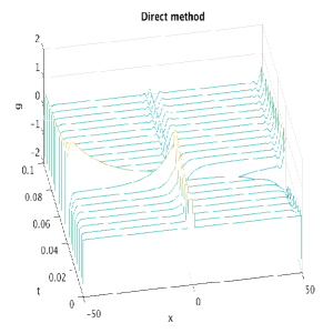
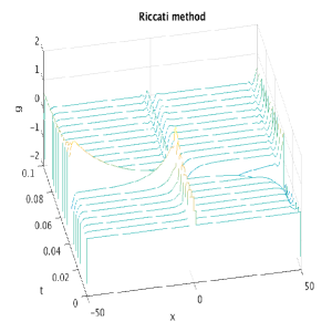
Figure 1: We plot the solution to the nonlocal quadratically nonlinear partial differential equation from Example 1. We used a generic initial profile $g_{0}$ as shown. The left panel shows the solution computed using a direct integration approach while the right panel shows the solution computed using our Riccati approach.

Remark 6 (Multi-dimensions)

This last example extends to the case where $x,y\in{\mathbb{R}}^{n}$ for any $n\geqslant 1$ when $d$ is a scalar operator such as a power of the Laplacian, with $p$, $q^{\prime}$ and $g$ all scalar.

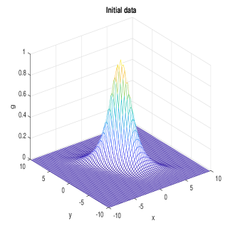
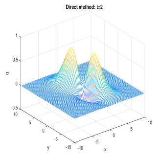
Figure 2: We plot the solution to the nonlocal quadratically nonlinear partial differential equation with correlation from Example 2. We used a generic initial profile $g_{0}$ as shown in the top panel. For time $t=2$, the middle panel shows the solution computed using a direct integration approach while the bottom panel shows the solution computed using our Riccati approach.

Example 2 (Nonlocal quadratic nonlinearity with correlation)

In this case the target evolutionary partial differential equation has a nonlocal quadratic nonlinearity involving a correlation function and has the form

$${\partial}_{t}g(x,y;t)=d({\partial}_{x})\,g(x,y;t)-\int_{{\mathbb{R}}}g(x,z;t)\,b(z)\,g(z,y;t)\,{\mathrm{d}}z.$$

This corresponds to the evolutionary partial differential equation with nonlocal quadratic nonlinearity in Corollary 3.1, with $a=c=0$ and $b=b(x)$ the scalar smooth, bounded square-integrable function described in the paragraphs preceding it. We also assume that $d=d({\partial}_{x})$ is of the diffusive or dispersive form described in Remark 4. We assume smooth and square-integrable initial data $g_{0}=g_{0}(x,y)$.

To find solutions to the evolutionary partial differential equation just above using our approach we assume the linear base and auxiliary equations have the form

$${\partial}_{t}p(x,y;t) =d(\partial_{x})\,p(x,y;t),$$

$${\partial}_{t}q^{\prime}(x,y;t) =b(x)\,p(x,y;t).$$

In Fourier space the solution of the base equation has the form

$$\hat{p}(k,y;t)=\mathrm{e}^{d(2\pi\mathrm{i}k)\,t}\,\hat{p}_{0}(k,y),$$

where $\hat{p}_{0}$ is the Fourier transform of the initial data for $p$. The auxiliary equation solution in Fourier space has the form,

$$\hat{q}^{\prime}(k,y;t)=\int_{\mathbb{R}}\hat{b}(k-\kappa)\,\hat{I}(\kappa,t)\,\hat{p}_{0}(\kappa,y)\,{\mathrm{d}}\kappa,$$

where we set

$$\hat{I}(k,t)\coloneqq\frac{\mathrm{e}^{d(2\pi\mathrm{i}k)\,t}-1}{d(2\pi\mathrm{i}k)}.$$

As in the last example we took the initial data for $q^{\prime}$ to be zero and thus the initial data for $\hat{q}^{\prime}$ is also zero. We also set the initial data for $p=p(x,y;t)$ to be $p_{0}(x,y)=g_{0}(x,y)$. In Fourier space this is equivalent to $\hat{p}_{0}(k,y)=\hat{g}_{0}(k,y)$. We now derive an explicit form for $q^{\prime}=q^{\prime}(x,y;t)$ from $\hat{q}^{\prime}=\hat{q}^{\prime}(k,y;t)$ above. Taking the inverse Fourier transform of $\hat{q}^{\prime}$, we find that

$$q^{\prime}(x,y;t)= \;\int_{\mathbb{R}}\biggl{(}\int_{\mathbb{R}}\mathrm{e}^{-2\pi\mathrm{i}kx}\,\hat{b}(k-\kappa)\,{\mathrm{d}}k\biggr{)}\hat{I}(\kappa,t)\,\hat{g}_{0}(\kappa,y)\,{\mathrm{d}}\kappa$$

$$= \;\int_{\mathbb{R}}\bigl{(}\mathrm{e}^{-2\pi\mathrm{i}\kappa x}\,b(x)\bigr{)}\hat{I}(\kappa,t)\,\hat{g}_{0}(\kappa,y)\,{\mathrm{d}}\kappa$$

$$= \;b(x)\int_{\mathbb{R}}\mathrm{e}^{-2\pi\mathrm{i}\kappa x}\,\hat{I}(\kappa,t)\,\hat{g}_{0}(\kappa,y)\,{\mathrm{d}}\kappa$$

$$= \;b(x)\int_{\mathbb{R}}I(x-\zeta,t)\,g_{0}(\zeta,y)\,{\mathrm{d}}\zeta.$$

Lastly, the Riccati relation here has the form

$$p(x,y;t)=g(x,y;t)+\int_{{\mathbb{R}}}g(x,z;t)\,q^{\prime}(z,y;t)\,{\mathrm{d}}z.$$

Since we have an explicit expression for $q^{\prime}=q^{\prime}(x,y;t)$, and we can obtain one for $p=p(x,y;t)$ by taking the inverse Fourier transform of the explicit expression for $\hat{p}=\hat{p}(k,y;t)$ above, we can solve this linear Fredholm equation for $g=g(x,y;t)$. The solution, by Corollary 3.1, will be the solution to the evolutionary partial differential equation with the nonlocal quadratic nonlinearity above corresponding to the initial data $g_{0}(x,y)$.

We solved the Fredholm equation for $g=g(x,y;t)$ numerically. The results are shown in Figure 2. We set the operator $d=\partial_{x}^{2}+1$ and took as the generic initial profile $g_{0}(x,y)\coloneqq\mathrm{sech}(x+y)\,\mathrm{sech}(y)$. We set $b=b(x)$ to be a mean-zero Gaussian density function with standard deviation $0.01$. The top panel in Figure 2 shows the initial data. The middle panel in the figure shows the solution profile computed at time $t=2$ using a direct spectral integration approach. By this we mean we solved the equation for $\hat{g}(k,y;t)$ generated by taking the Fourier transform of the equation for $g=g(x,y;t)$. We used the inbuilt Matlab integrator ode23s to integrate in time. The bottom panel in Figure 2 shows the solution computed with the time parameter $t=2$ using our Riccati approach, i.e. by numerically solving the Fredholm equation for $g=g(x,y;t)$ above by standard methods for such integral equations. As expected, the solutions in the middle and bottom panels look identical (up to numerical precision).

Remark 7

We emphasize that, when we can explicitly solve for $p=p(x,y;t)$ and $q^{\prime}=q^{\prime}(x,y;t)$ in our Riccati approach, then time $t$ plays the role of a parameter. One decides the time at which one wants to compute the solution and we then solve the Fredholm equation to generate the solution $g=g(x,y;t)$ for that time $t$. This is one of the advantages of our method over standard numerical schemes.

Remark 8 (Burgers’ equation)

Burgers’ equation can be considered as a special case of our Riccati approach in the following sense. Suppose the linear base and auxiliary equations are ${\partial}_{t}p(x;t)={\partial}_{x}^{2}p(x;t)$ and ${\partial}_{t}q(x;t)={\partial}_{x}p(x;t)$ for the real valued functions $p$ and $q$. Further suppose the Riccati relation takes the form $p(x;t)=g(x;t)\,q(x;t)$ where $g$ is also real valued. Note this represents a rank one relation between $p$ and $q$ in the sense that we obtain $p$ from $q$ by a simple multiplication of $q$ by the function $g$. From the linear base and auxiliary equations, assuming smooth solutions, we deduce that ${\partial}_{t}q={\partial}_{x}p={\partial}_{x}^{-1}{\partial}_{x}^{2}p={\partial}_{x}^{-1}{\partial}_{t}p={\partial}_{t}({\partial}_{x}^{-1}p)$, where ${\partial}_{x}^{-1}w$ represents the operation $\int_{-\infty}^{x}w(z)\,{\mathrm{d}}z$ for any smooth integrable function $w=w(x)$ on ${\mathbb{R}}$. From the above equalities we deduce $p(x;t)={\partial}_{x}q(x;t)+f(x)$ where $f=f(x)$ is an arbitrary function of $x$ only. If we take the special case $f\equiv 0$, then we deduce $p(x;t)={\partial}_{x}q(x;t)$. This also implies ${\partial}_{t}q={\partial}_{x}^{2}q$. If we insert the relation $p(x;t)={\partial}_{x}q(x;t)$ into the Riccati relation we find

$$g(x;t)=\frac{{\partial}_{x}q(x;t)}{q(x;t)}.$$

This is almost the Cole–Hopf transformation, its just missing the usual ‘-2’ factor on the right-hand side. However carrying through our Riccati approach by direct computation, differentiating the Riccati relation with respect to time, we observe

$$({\partial}_{t}g)\,q ={\partial}_{t}p-g\,{\partial}_{t}q$$

$$={\partial}_{x}^{2}p-g\,{\partial}_{t}q$$

$$={\partial}_{x}^{2}(g\,q)-g\,{\partial}_{t}q$$

$$=({\partial}_{x}^{2}g)\,q+2\,({\partial}_{x}g)\,{\partial}_{x}q+g\,({\partial}_{x}^{2}q)-g\,{\partial}_{t}q$$

$$=({\partial}_{x}^{2}g)\,q+2\,({\partial}_{x}g)\,p$$

$$=({\partial}_{x}^{2}g)\,q+2\,({\partial}_{x}g)\,g\,q.$$

If we divide through by the function $q=q(x;t)$ we conclude that $g=g(x;t)$ satisfies the nonlinear partial differential equation

$${\partial}_{t}g={\partial}_{x}^{2}g+2\,g\,{\partial}_{x}g.$$

However we now observe that ‘$-2\,g$’ indeed satisfies Burgers’ equation.

5 Conclusions

There are many extensions of our approach to more general nonlinear partial differential equations. One immediate extension to consider is to multi-dimensions, i.e. where the underlying spatial domain lies in ${\mathbb{R}}^{n}$ for some $n\geqslant 1$. This should be straightforward as indicated in Remark 6 above. Another immediate extension is to systems of nonlinear partial differential equations with nonlocal nonlinearites. Indeed we explicitly consider this extension in Beck, Doikou, Malham and Stylianidis BDMStrans where we demonstrate how to generate solutions to certain classes of reaction-diffusion systems with nonlocal quadratic nonlinearities. We also demonstrate therein, how to extend our approach to generate solutions to evolutionary partial differential equations with higher degree nonlocal nonlinearities, including the nonlocal nonlinear Schrödinger equation. Further therein, for arbitrary initial data $g_{0}=g_{0}(x)$, we use our Riccati approach to generate solutions to the nonlocal Fisher–Kolmogorov–Petrovskii–Piskunov equation for scalar $g=g(x;t)$ of the form

$${\partial}_{t}g(x;t)=d({\partial}_{x})\,g(x;t)-g(x;t)\int_{\mathbb{R}}g(z;t)\,{\mathrm{d}}z.$$

This has recently received some attention; see Britton Britton and Bian, Chen and Latos BCL . We would also like to consider the extension of our approach to the full range of possible choices of the operators $d$ and $b$ both as unbounded and bounded operators, for example to fractional and nonlocal diffusion cases. We have already considered the extension of our approach to evolutionary stochastic partial differential equations with nonlocal nonlinearities in Doikou, Malham and Wiese DMW . Therein we consider the separate cases when the driving space-time Wiener field appears as a nonhomogeneous additive source term or as a multiplicative but linear source term. Of course, another natural extension is to determine whether we can include the generation of solutions to evolutionary partial differential equations with local nonlinearities within the context of our Riccati approach. One potential approach is to suppose the Riccati relation is of Volterra type. This is an ongoing investigation. Lastly we remark that for the classes of nonlinear partial differential equations we can consider, solution singularities correspond to poor choices of coordinate patches which are related to function space regularity. In principle solutions can be continued by changing coordinate patches; see Schiff and Shnider SchiffShnider and Ledoux et al. LMT . This is achieved by pulling back the flow to the relevant general linear group and then projecting down to a more appropriate coordinate patch of the Fredholm Grassmannian. Alternatively, we could continue the flow in the appropriate general linear group via the base and auxiliary equations, and then monitor the relevant projection(s).

- (1) Abbondandolo, A, Majer, P, 2009 Infinite dimensional Grassmannians, J. Operator Theory 61(1), 19–62.
- (2) Ablowitz, MJ, Ramani, A, Segur, H. 1980 A connection between nonlinear evolution equations and ordinary differential equations of P-type. I, Journal of Mathematical Physics 21, 715–721.
- (3) Ablowitz, MJ, Ramani, A, Segur, H. 1980 A connection between nonlinear evolution equations and ordinary differential equations of P-type. II, Journal of Mathematical Physics 21, 1006–1015.
- (4) Ablowitz, MJ, Zeppetella, A. 1979 Explicit solutions of Fisher’s equation for a special wave speed, Bulletin of Mathematical Biology 41, 835–840.
- (5) Alexander, JC, Gardner, R, Jones, CKRT. 1990 A topological invariant arising in the stability analysis of traveling waves, J. Reine Angew. Math. 410, 167–212.
- (6) Balazs, P. 2008 Hilbert–Schmidt operators and frames—classification, best approximation by multipliers and algorithms, International Journal of Wavelets, Multiresolution and Information Processing 6(2), 315–330.
- (7) Bauhardt, W, Pöppe, Ch. 1993 The Zakharov–Shabat inverse spectral problem for operators, J. Math, Phys. 34(7), 3073–3086.
- (8) Beals, R, Coifman, RR. 1989 Linear spectral problems, non-linear eqautions and the -method, Inverse problems 5, 87–130.
- (9) Beck M, Doikou A, Malham SJA, Stylianidis I. 2017 Partial differential systems with nonlocal nonlinearities: Generation and solution, Phil. Trans. A, accepted.
- (10) Beck M, Malham SJA. 2015 Computing the Maslov index for large systems, PAMS 143, 2159–2173.
- (11) Bian S, Chen L, Latos EA. 2017 Global existence and asymptotic behavior of solutions to a nonlocal Fisher–KPP type problem, Nonlinear Analysis 149, 165-–176.
- (12) Bittanti, S, Laub, AJ, Willems, JC. (Eds.) 1991 The Riccati equation, Communications and Control Engineering Series, Springer–Verlag.
- (13) Blanchard, P, Brüning, E. 2015 Mathematical methods in Physics: Distributions, Hilbert space operators, variational methods, and applications in quantum physics, Progress in Mathematical Physics 69, Second Edition, Birkhäuser.
- (14) Bornemann, F. 2009 Numerical evaluation of Fredholm determinants and Painlevé transcendents with applications to random matrix theory, talk at the Abdus Salam International Centre for Theoretical Physics.
- (15) Britton NF. 1990 Spatial structures and periodic travelling waves in an integro-differential reaction-diffusion population model, SIAM J. Appl. Math. 50(6), 1663–1688.
- (16) Brockett RW, Byrnes CI. 1981 Multivariable Nyquist criteria, root loci, and pole placement: a geometric viewpoint, IEEE Trans. Automat. control 26(1), 271–284.
- (17) Christensen, O. 2008 Frames and Bases, Springer. DOI: 10.1007/978-0-8176-4678-3_3.
- (18) Deng J, Jones, C. 2011 Multi-dimensional Morse index theorems and a symplectic view of elliptic boundary value problems, Transactions of the American Mathematical Society 363(3), 1487–1508.
- (19) Dodd, RK, Eilbeck, JC, Gibbon, JD, Morris HC. 1982 Solitons and non-linear wave equations, London, Academic Press.
- (20) Doikou A, Malham SJA, Wiese A. 2018 Stochastic partial differential equations with nonlocal nonlinearities and their simulation, in preparation.
- (21) Drazin, PG, Johnson, RS. 1989 Solitons: an introduction, Cambridge Texts in Applied Mathematics, Cambridge University Press.
- (22) Dyson, FJ. 1976 Fredholm determinants and inverse scattering problems, Commun. Math. Phys. 47, 171–183.
- (23) Furutani, K. 2004 Review: Fredholm–Lagrangian–Grassmannian and the Maslov index, Journal of Geometry and Physics 51, 269–331.
- (24) Grellier, S, Gerard, P. 2015 The cubic Szegö equation and Hankel operators, arXiv:1508.06814.
- (25) Griffiths, P, Harris, J. 1994 Principles of Algebraic geometry, Wiley Classics Library.
- (26) Guest, MA. 2008 From quantum cohomology to integrable systems, Oxford University Press.
- (27) Hermann, R. 1979 Cartanian geometry, nonlinear waves, and control theory: Part A, Interdisciplinary Mathematics Vol. XX, Math Sci Press.
- (28) Hermann, R. 1980 Cartanian geometry, nonlinear waves, and control theory: Part B, Interdisciplinary Mathematics Vol. XXI, Math Sci Press.
- (29) Hermann R, Martin C. 1982 Lie and Morse theory for periodic orbits of vector fields and matrix Riccati equations, I: General Lie-theoretic methods, Math. Systems Theory 15, 277-–284.
- (30) Karambal I, Malham SJA. 2015 Evans function and Fredholm determinants, Proc. R. Soc. A 471(2174). DOI: 10.1098/rspa.2014.0597
- (31) McKean, HP. 2011 Fredholm determinants, Cent. Eur. J. Math. 9(2), 205–243.
- (32) Ledoux, V, Malham, SJA, Niesen, J, Thümmler, V. 2009 Computing stability of multi-dimensional travelling waves, SIAM Journal on Applied Dynamical Systems 8(1), 480–507.
- (33) Ledoux, V, Malham, SJA, Thümmler, V. 2010 Grassmannian spectral shooting, Math. Comp. 79, 1585–1619.
- (34) Martin C, Hermann R. 1978 Applications of algebraic geometry to systems theory: The McMillan degree and Kronecker indicies of transfer functions as topological and holomorphic system invariants, SIAM J. Control Optim. 16(5), 743–755.
- (35) Miura, RM. 1976 The Korteweg–De Vries equation: A survey of results, SIAM Review 18(3), 412–459.
- (36) Miwa, T, Jimbo, M, Date, E. 2000 Solitons: Differential equations, symmetries and infinite dimensional algebras, Cambridge University Press.
- (37) Piccione, P, Tausk, DV. 2008 A Student’s Guide to Symplectic Spaces, Grassmannians and Maslov Index, www.ime.usp.br/piccione/Downloads/MaslovBook.pdf
- (38) Pöppe, Ch. 1983 Construction of solutions of the sine-Gordon equation by means of Fredholm determinants, Physica D 9, 103–139.
- (39) Pöppe, Ch. 1984 The Fredholm determinant method for the KdV equations, Physica D 13, 137–160.
- (40) Pöppe, Ch. 1984 General determinants and the function for the Kadomtsev–Petviashvili hierarchy, Inverse Problems 5, 613–630.
- (41) Pöppe, Ch., Sattinger, D.H. 1988 Fredholm determinants and the function for the Kadomtsev–Petviashvili hierarchy, Publ. RIMS, Kyoto Univ. 24, 505–538.
- (42) Pressley, A., Segal, G. 1986 Loop groups, Oxford Mathematical Monographs, Clarendon Press, Oxford.
- (43) Reed, M., Simon, B. 1980, Methods of Modern Mathematical Physics: I Functional Analysis, Academic Press.
- (44) Sato, M. 1981 Soliton equations as dynamical systems on a infinite dimensional Grassmann manifolds. RIMS 439, 30–46.
- (45) Sato, M. 1989, The KP hierarchy and infinite dimensional Grassmann manifolds, Proceedings of Symposia in Pure Mathematics 49 Part 1, 51–66.
- (46) Schiff J., Shnider, S. 1999 A natural approach to the numerical integration of Riccati differential equations, SIAM J. Numer. Anal. 36(5), 1392–1413.
- (47) Segal, G., Wilson, G. 1985 Loop groups and equations of KdV type, Inst. Hautes Etudes Sci. Publ. Math. N61, 5-–65.
- (48) Simon, B. 2005 Trace ideals and their applications, 2nd edn. Mathematical Surveys and Monographs, vol. 120. Providence, RI: AMS.
- (49) Tracy, C.A., Widom, H. 1996 Fredholm determinants and the mKdV/Sinh-Gordon hierarchies, Commun. Math. Phys. 179, 1–10.
- (50) Wilson, G. 1985 Infinite-dimensional Lie groups and algebraic geometry in soliton theory, Trans. R. Soc. London A 315 (1533), 393–404.
- (51) Zakharov, V.E., Shabat, A.B. 1974 A scheme for integrating the non-linear equation of mathematical physics by the method of the inverse scattering problem I, Funct. Anal. Appl. 8, 226.
- (52) Zelikin, M.I. 2000 Control theory and optimization I, Encyclopedia of Mathematical Sciences Vol. 86, Springer–Verlag.