The hyperbolic geometry of Markov’s theorem on Diophantine approximation and quadratic forms

Abstract

Markov’s theorem classifies the worst irrational numbers with respect to rational approximation and the indefinite binary quadratic forms whose values for integer arguments stay farthest away from zero. The main purpose of this paper is to present a new proof of Markov’s theorem using hyperbolic geometry. The main ingredients are a dictionary to translate between hyperbolic geometry and algebra/number theory, and some very basic tools borrowed from modern geometric Teichmüller theory. Simple closed geodesics and ideal triangulations of the modular torus play an important role, and so do the problems: How far can a straight line crossing a triangle stay away from the vertices? How far can it stay away from the vertices of the tessellation generated by the triangle? Definite binary quadratic forms are briefly discussed in the last section.

MSC (2010). 11J06, 32G15
Key words and phrases. Diophantine approximation, quadratic form, modular torus, closed geodesic

1 Introduction

The main purpose of this article is to present a new proof of Markov’s theorem [49, 50] (Secs. 2, 3) using hyperbolic geometry. Roughly, the following dictionary is used to translate between hyperbolic geometry and algebra/number theory:

Hyperbolic Geometry	Algebra/Number Theory
horocycle	nonzero vector $(p,q)\in\mathbb{R}^{2}$	Sec. 5
geodesic	indefinite binary quadratic form $f$	Sec. 10
point	definite binary quadratic form $f$	Sec. 16
signed distance between horocycles	$2\log\Big{|}\det\Big{(}\begin{smallmatrix}p_{1}&p_{2}\\ q_{1}&q_{2}\end{smallmatrix}\Big{)}\Big{|}$	(24)
signed distance between horocycle and geodesic/point	$\displaystyle\log\frac{f(p,q)}{\sqrt{|\det f|}}$	(29) (46)
ideal triangulation of the modular torus	Markov triple	Sec. 12

The proof is based on Penner’s geometric interpretation of Markov’s equation [56, p. 335f] (Sec. 12), and the main tools are borrowed from his theory of decorated Teichmüller space (Sec. 11). Ultimately, the proof of Markov’s theorem boils down to the question:

How far can a straight line crossing a triangle stay away from all vertices?

It is fun and a recommended exercise to consider this question in elementary euclidean geometry. Here, we need to deal with ideal hyperbolic triangles, decorated with horocycles at the vertices, and “distance from the vertices” is to be understood as “signed distance from the horocycles” (Sec. 13).

The subjects of this article, Diophantine approximation, quadratic forms, and the hyperbolic geometry of numbers, are connected with diverse areas of mathematics and its applications, ranging from from the phyllotaxis of plants [16] to the stability of the solar system [38], and from Gauss’ Disquisitiones Arithmeticae to Mirzakhani’s Fields Medal [54]. An adequate survey of this area, even if limited to the most important and most recent contributions, would be beyond the scope of this introduction. The books by Aigner [2] and Cassels [11] are excellent references for Markov’s theorem, Bombieri [6] provides a concise proof, and more about the Markov and Lagrange spectra can be found in Malyshev’s survey [48] and the book by Cusick and Flahive [20]. The following discussion focuses on a few historic sources and the most immediate context and is far from comprehensive.

One can distinguish two approaches to a geometric treatment of continued fractions, Diophantine approximation, and quadratic forms. In both cases, number theory is connected to geometry by a common symmetry group, $\mathit{GL}_{2}(\mathbb{Z})$. The first approach, known as the geometry of numbers and connected with the name of Minkowski, deals with the geometry of the $\mathbb{Z}^{2}$-lattice. Klein interpreted continued fraction approximation, intuitively speaking, as “pulling a thread tight” around lattice points [42, 43]. This approach extends naturally to higher dimensions, leading to a multidimensional generalization of continued fractions that was championed by Arnold [3, 4]. Delone’s comments on Markov’s work [22] also belong in this category (see also [30]).

In this article, we pursue the other approach involving Ford circles and the Farey tessellation of the hyperbolic plane (Fig. 6). This approach could be called the hyperbolic geometry of numbers. Before Ford’s geometric proof [28] of Hurwitz’s theorem [39] (Sec. 2), Speiser had apparently used the Ford circles to prove a weaker approximation theorem. However, only the following note survives of his talk [71, my translation]:

A geometric figure related to number theory. If one constructs in the upper half plane for every rational point of the $x$-axis with abscissa $\frac{p}{q}$ the circle of radius $\frac{1}{2q^{2}}$ that touches this point, then these circles do not overlap anywhere, only tangencies occur. The domains that are not covered consist of circular triangles. Following the line $x=\omega$ (irrational number) downward towards the $x$-axis, one intersects infinitely many circles, i.e., the inequality

$$\big{|}\omega-\frac{p}{q}\big{|}<\frac{1}{2q^{2}}$$

has infinitely many solutions. They constitute the approximations by Minkowski’s continued fractions.

If one increases the radii to $\frac{1}{\sqrt{3}q^{2}}$, then the gaps close and one obtains the theorem on the maximum of positive binary quadratic forms.

See Rem. 9.2 and Sec. 16 for brief comments on these theorems. Based on Speiser’s talk, Züllig [76] developed a comprehensive geometric theory of continued fractions, including a geometric proof of Hurwitz’s theorem.

Both Züllig and Ford treat the arrangement of Ford circles using elementary euclidean geometry and do not mention any connection with hyperbolic geometry. In Sec. 9, we transfer their proof of Hurwitz’s theorem to hyperbolic geometry. The conceptual advantage is obvious: One has to consider only three circles instead of infinitely many, because all triples of pairwise touching horocycles are congruent.

Today, the role of hyperbolic geometry is well understood. Continued fraction expansions encode directions for navigating the Farey tessellation of the hyperbolic plane [7, 34, 68]. In fact, much was already known to Hurwitz [40] and Klein [41, 43]. According to Klein [43, p. 248], they built on Hermite’s [36] purely algebraic discovery of an invariant “incidence” relation between definite and indefinite forms, which they translated into the language of geometry. While Hurwitz and Klein never mention horocycles, they knew the other entries of the dictionary, and even use the Farey triangulation. In the Cayley–Klein model of hyperbolic space, the geometric interpretation of binary quadratic forms is easily established: The projectivized vector space of real binary quadratic forms is a real projective plane and the degenerate forms are a conic section. Definite forms correspond to points inside this conic, hence to points of the hyperbolic plane, while indefinite forms correspond to points outside, hence, by polarity, to hyperbolic lines. From this geometric point of view, Klein and Hurwitz discuss classical topics of number theory like the reduction of binary quadratic forms, their automorphisms, and the role of Pell’s equation. Strangely, it seems they never treated Diophantine approximation or Markov’s work this way.

Cohn [12] noticed that Markov’s Diophantine equation (4) can easily be obtained from an elementary identity of Fricke involving the traces of $2\times 2$-matrices. Based on this algebraic coincidence, he developed a geometric interpretation of Markov forms as simple closed geodesics in the modular torus [13, 14], which is also adopted in this article.

A much more geometric interpretation of Markov’s equation was discovered by Penner (as mentioned above), as a byproduct of his decorated Teichmüller theory [56, 57]. This interpretation focuses on ideal triangulations of the modular torus, decorated with a horocycle at the cusp, and the weights of their edges (Sec. 12). Penner’s interpretation also explains the role of simple closed geodesics (Sec. 14).

Markov’s original proof (see [6] for a concise modern exposition) is based on an analysis of continued fraction expansions. Using the interpretation of continued fractions as directions in the Farey tessellation mentioned above, one can translate Markov’s proof into the language of hyperbolic geometry. The analysis of allowed and disallowed subsequences in an expansion translates to symbolic dynamics of geodesics [67].

In his 1953 thesis, which was published much later, Gorshkov [31] provided a genuinely new proof of Markov’s theorem using hyperbolic geometry. It is based on two important ideas that are also the foundation for the proof presented here. First, Gorshkov realized that one should consider all ideal triangulations of the modular torus, not only the projected Farey tessellation. This reduces the symbolic dynamics argument to almost nothing (in this article, see Proposition 15.1, the proof of implication “$\text{(c)}\Rightarrow\text{(a)}$”). Second, he understood that Markov’s theorem is about the distance of a geodesic to the vertices of a triangulation. However, lacking modern geometric tools of Teichmüller theory (like horocycles), Gorshkov was not able to treat the geometry of ideal triangulations directly. Instead, he considers compact tori composed of two equilateral hyperbolic triangles and lets the side length tend to infinity. The compact tori have a cone-like singularity at the vertex, and the developing map from the punctured torus to the hyperbolic plane has infinitely many sheets. This limiting process complicates the argument considerably. Also, the trigonometry becomes simpler when one needs to consider only decorated ideal triangles. Gorshkov’s decision “not to restrict the exposition to the minimum necessary for proving Markov’s theorem but rather to execute it with considerable completeness, retaining everything that is of independent interest” makes it harder to recognize the main lines of argument. This, together with an unduly dismissive MathSciNet review, may account for the lack of recognition his work received.

In this article, we adopt the opposite strategy and stick to proving Markov’s theorem. Many natural generalizations and related topics are beyond the scope of this paper, for example the approximation of complex numbers [21, 26, 27, 62], generalizations to other Riemann surfaces or discrete groups [1, 5, 9, 32, 47, 63, 64], higher dimensional manifolds [37, 74], other Diophantine approximation theorems, for example Khinchin’s [72], and the asymptotic growth of Markov numbers and lengths of closed geodesics [8, 51, 53, 69, 70, 75]. Is the treatment of Markov’s equation using $3\times 3$-matrices [58, 60] related? Do the methods presented here help to cover a larger part of the Markov and Lagrange spectra by considering more complicated geodesics [17, 18, 19]? Can one treat, say, ternary quadratic forms or binary cubic forms in a similar fashion?

The notorious Uniqueness Conjecture for Markov numbers (Rem. 2.1 (iv)), which goes back to a neutral statement by Frobenius [29, p. 461], says in geometric terms: If two simple closed geodesics in the modular torus have the same length, then they are related by an isometry of the modular torus [66]. Equivalently, if two ideal arcs have the same weight, they are related this way. Hyperbolic geometry was instrumental in proving the uniqueness conjecture for Markov numbers that are prime powers [10, 45, 65]. Will geometry also help to settle the full Uniqueness Conjecture, or is it “a conjecture in pure number theory and not tractable by hyperbolic geometry arguments” [52]? Will combinatorial methods succeed? Who knows. These may not even be very meaningful questions, like asking: “Will a proof be easier in English, French, Russian, or German?” On the other hand, sometimes it helps to speak more than one language.

2 The worst irrational numbers

There are two versions of Markov’s theorem. One deals with Diophantine approximation, the other with quadratic forms. In this section, we recall some related theorems and state the Diophantine approximation version in the form in which we will prove it (Sec. 15). The following section is about the quadratic forms version.

Let $x$ be an irrational number. For every positive integer $q$ there is obviously a fraction $\frac{p}{q}$ that approximates $x$ with error less than $\smash[b]{\frac{1}{2q}}$. If one chooses denominators more carefully, one can find a sequence of fractions converging to $x$ with error bounded by $\smash[t]{\frac{1}{q^{2}}}$:

Theorem.

For every irrational number $x$, there are infinitely many fractions $\frac{p}{q}$ satisfying

$$\Big{|}x-\frac{p}{q}\Big{|}<\frac{1}{q^{2}}\,.$$

This theorem is sometimes attributed to Dirichlet although the statement had “long been known from the theory of continued fractions” [23]. In fact, Dirichlet provided a particularly simple proof of a multidimensional generalization, using what later became known as the pigeonhole principle.

Klaus Roth was awarded a Fields Medal in 1958 for showing that the exponent $2$ in Dirichlet’s approximation theorem is optimal [61]:

Theorem (Roth).

Suppose $x$ and $\alpha$ are real numbers, $\alpha>2$. If there are infinitely many reduced fractions $\frac{p}{q}$ satisfying

$$\Big{|}x-\frac{p}{q}\Big{|}<\frac{1}{q^{\alpha}}\,,$$

then $x$ is transcendental.

In other words, if the exponent in the error bound is greater than $2$ then algebraic irrational numbers cannot be approximated. This is an example of a general observation: “From the point of view of rational approximation, the simplest numbers are the worst” (Hardy & Wright [33], p. 209, their emphasis). Roth’s theorem shows that the worst irrational numbers are algebraic. Markov’s theorem, which we will state shortly, shows that the worst algebraic irrationals are quadratic.

While the exponent is optimal, the constant factor in Dirichlet’s approximation theorem can be improved. Hurwitz [39] showed that the optimal constant is $\frac{1}{\sqrt{5}}$, and that the golden ratio belongs to the class of very worst irrational numbers:

Theorem (Hurwitz).

(i) For every irrational number $x$, there are infinitely many fractions $\frac{p}{q}$ satisfying

$$\Big{|}x-\frac{p}{q}\Big{|}<\frac{1}{\sqrt{5}\,q^{2}}\,.$$ (1)

(ii) If $\lambda>\sqrt{5}$, and if $x$ is equivalent to the golden ratio $\phi=\frac{1}{2}(1+\sqrt{5})$, then there are only finitely many fractions $\frac{p}{q}$ satisfying

$$\Big{|}x-\frac{p}{q}\Big{|}<\frac{1}{\lambda\,q^{2}}\,.$$ (2)

Two real numbers $x$, $x^{\prime}$ are called equivalent if

$$x^{\prime}=\frac{ax+b}{cx+d},$$ (3)

for some integers $a$, $b$, $c$, $d$ satisfying

$$|ad-bc|=1.$$

If infinitely many fractions satisfy (2) for some $x$, then the same is true for any equivalent number $x^{\prime}$. This follows simply from the identity

$$(q^{\prime})^{2}\,\Big{|}x^{\prime}-\frac{p^{\prime}}{q^{\prime}}\Big{|}=q^{2}\,\Big{|}x-\frac{p}{q}\Big{|}\;\frac{\big{|}c\,\big{(}\frac{p}{q}\big{)}+d\big{|}}{\big{|}cx+d\big{|}},$$

where $x$ and $x^{\prime}$ are related by (3) and $p^{\prime}=ap+bq$, $q^{\prime}=cp+dq$. (Note that the last factor on the right hand side tends to $1$ as $\frac{p}{q}$ tends to $x$.)

Hurwitz also states the following results, “whose proofs can easily be obtained from Markov’s investigation” of indefinite quadratic forms:

$\bullet$ If $x$ is an irrational number not equivalent to the golden ratio $\phi$, then infinitely many fractions satisfy (2) with $\lambda=2\sqrt{2}$.

$\bullet$ For any $\lambda<3$, there are only finitely many equivalence classes of numbers that cannot be approximated, i.e., for which there are only finitely many fractions satisfying (2). But for $\lambda=3$, there are infinitely many classes that cannot be approximated.

Hurwitz stops here, but the story continues. Table 1 lists representatives $x$ of the five worst classes of irrational numbers, and the largest values $L(x)$ for $\lambda$ for which there exist infinitely many fractions satisfying (2). For example, $\sqrt{2}$ belongs to the class of second worst irrational numbers. The last two columns will be explained in the statement of Markov’s theorem.

rank	$x$	$L(x)$		$\ a$	$\ b$	$\ c$	$\ p_{1}$	$\ p_{2}$
1	$\frac{1}{2}(1+\sqrt{5})$	$\sqrt{5}$$\;=\;$	$2.2\ldots$	$1$	$1$	$1$	$0$	$1$
2	$\sqrt{2}$	$2\sqrt{2}$$\;=\;$	$2.8\ldots$	$1$	$1$	$2$	$-1$	$1$
3	$\frac{1}{10}(9+\sqrt{221})$	$\frac{1}{5}\sqrt{221}$$\;=\;$	$2.97\ldots$	$1$	$2$	$5$	$-1$	$2$
4	$\frac{1}{26}(23+\sqrt{1517})$	$\frac{1}{13}\sqrt{1517}$$\;=\;$	$2.996\ldots$	$1$	$5$	$13$	$-3$	$2$
5	$\frac{1}{58}(5+\sqrt{7565})$	$\frac{1}{29}\sqrt{7565}$$\;=\;$	$2.9992\ldots$	$2$	$5$	$29$	$-7$	$3$

Table 1: The five worst classes of irrational numbers

Markov’s theorem establishes an explicit bijection between the equivalence classes of the worst irrational numbers, and sorted Markov triples. Here, worst irrational numbers means precisely those that cannot be approximated for some $\lambda<3$. A Markov triple is a triple $(a,b,c)$ of positive integers satisfying Markov’s equation

$$a^{2}+b^{2}+c^{2}=3abc.$$ (4)

A Markov number is a number that appears in some Markov triple. Any permutation of a Markov triple is also a Markov triple. A sorted Markov triple is a Markov triple $(a,b,c)$ with $a\leq b\leq c$.

We review some basic facts about Markov triples and refer to the literature for details, for example [2, 11]. First and foremost, note that Markov’s equation (4) is quadratic in each variable. This allows one to generate new solutions from known ones: If $(a,b,c)$ is a Markov triple, then so are its neighbors

$$(a^{\prime},b,c),\quad(a,b^{\prime},c),\quad(a,b,c^{\prime}),$$ (5)

where

$$a^{\prime}=3bc-a=\frac{b^{2}+c^{2}}{a},$$ (6)

and similarly for $b^{\prime}$ and $c^{\prime}$. Hence, there are three involutions $\sigma_{k}$ on the set of Markov triples that map any triple $(a,b,c)$ to its neighbors:

$$\sigma_{1}(a,b,c)=(a^{\prime},b,c),\quad\sigma_{2}(a,b,c)=(a,b^{\prime},c),\quad\sigma_{3}(a,b,c)=(a,b,c^{\prime}).$$ (7)

These involutions act without fixed points and every Markov triple can be obtained from a single Markov triple, for example from $(1,1,1)$, by applying a composition of these involutions. The sequence of involutions is uniquely determined if one demands that no triple is visited twice. Thus, the solutions of Markov’s equation (4) form a trivalent tree, called the Markov tree, with Markov triples as vertices and edges connecting neighbors (see Fig. 1).

Figure 1: Markov tree

Theorem (Markov, Diophantine approximation version).

(i) Let $(a,b,c)$ be any Markov triple, let $p_{1}$, $p_{2}$ be integers satisfying

$$p_{2}b-p_{1}a=c,$$ (8)

and let

$$x=\frac{p_{2}}{a}+\frac{b}{ac}-\frac{3}{2}+\sqrt{\frac{9}{4}-\frac{1}{c^{2}}}\,.$$ (9)

Then there are infinitely many fractions $\frac{p}{q}$ satisfying (2) with

$$\lambda=\sqrt{9-\frac{4}{c^{2}}},$$ (10)

but only finitely many for any larger value of $\lambda$.

(ii) Conversely, suppose $x^{\prime}$ is an irrational number such that only finitely many fractions $\frac{p}{q}$ satisfy (2) for some $\lambda<3$. Then there exists a unique sorted Markov triple $(a,b,c)$ such that $x^{\prime}$ is equivalent to $x$ defined by equation (9).

Remark 2.1.

A few remarks, first some terminology.

(i) The Lagrange number $L(x)$ of an irrational number $x$ is defined by

$$L(x)=\sup\big{\{}\lambda\in\mathbb{R}\,\big{|}\,\text{infinitely many fractions $\tfrac{p}{q}$ satisfy\leavevmode\nobreak\ \eqref{eq:lambda}}\big{\}},$$

and the set of Lagrange numbers $\{L(x)\,|\,x\in\mathbb{R}\setminus\mathbb{Q}\}$ is called the Lagrange spectrum. Equation (10) describes the part of the Lagrange spectrum below $3$, and equation (9) provides representatives of the corresponding equivalence classes of irrational numbers.

(ii) It may seem strangely unsymmetric that $p_{2}$ appears in equation (9) and $p_{1}$ does not. The appearance is deceptive: Markov’s equation (4) and equation (8) imply that equation (9) is equivalent to

$$x=\frac{p_{1}}{b}-\frac{a}{bc}+\frac{3}{2}+\sqrt{\frac{9}{4}-\frac{1}{c^{2}}}\,.$$

(iii) The three integers of a Markov triple are pairwise coprime. (This is true for $(1,1,1)$, and if it is true for some Markov triple, then also for its neighbors.) Therefore, integers $p_{1}$, $p_{2}$ satisfying (8) always exist. Different solutions $(p_{1},p_{2})$ for the same Markov triple lead to equivalent values of $x$, differing by integers.

(iv) The following question is more subtle: Under what conditions do different Markov triples $(a,b,c)$ and $(a^{\prime},b^{\prime},c^{\prime})$ lead to equivalent numbers $x$, $x^{\prime}$? Clearly, if $c\not=c^{\prime}$, then $x$ and $x^{\prime}$ are not equivalent because $\lambda\not=\lambda^{\prime}$. But Markov triples $(a,b,c)$ and $(b,a,c)$ lead to equivalent numbers. In general, the numbers $x$ obtained by (9) from Markov triples $(a,b,c)$ and $(a^{\prime},b^{\prime},c^{\prime})$ are equivalent if and only if one can get from $(a,b,c)$ to $(a^{\prime},b^{\prime},c^{\prime})$ or $(b^{\prime},a^{\prime},c^{\prime})$ by a finite composition of the involutions $\sigma_{1}$ and $\sigma_{2}$ fixing $c$. In this case, let us consider the Markov triples equivalent. Every equivalence class of Markov triples contains exactly one sorted Markov triple. It is not known whether there exists only one sorted Markov triple $(a,b,c)$ for every Markov number $c$. This was remarked by Frobenius [29] some one hundred years ago, and the question is still open. The affirmative statement is known as the Uniqueness Conjecture for Markov Numbers. Consequently, it is not known whether there is only one equivalence class of numbers $x$ for every Lagrange number $L(x)<3$.

(v) The attribution of Hurwitz’s theorem may seem strange. It covers only the simplest part of Markov’s theorem, and Markov’s work precedes Hurwitz’s. However, Markov’s original theorem dealt with indefinite quadratic forms (see the following section). Despite its fundamental importance, Markov’s groundbreaking work gained recognition only very slowly. Hurwitz began translating Markov’s ideas to the setting of Diophantine approximation. As this circle of results became better understood by more mathematicians, the translation seemed more and more straightforward. Today, both versions of Markov’s theorem, the Diophantine approximation version and the quadratic forms version, are unanimously attributed to Markov.

3 Markov’s theorem on indefinite quadratic forms

In this section, we recall the quadratic forms version of Markov’s theorem.

We consider binary quadratic forms

$$f(p,q)=Ap^{2}+2Bpq+Cq^{2},$$ (11)

with real coefficients $A$, $B$, $C$. The determinant of such a form is the determinant of the corresponding symmetric $2\times 2$-matrix,

$$\det f=AC-B^{2}.$$ (12)

Markov’s theorem deals with indefinite forms, i.e., forms with

$$\det f<0.$$

In this case, the quadratic polynomial

$$f(x,1)=Ax^{2}+2Bx+C$$ (13)

has two distinct real roots,

$$\frac{-B\pm\sqrt{-\det f}}{A},$$ (14)

provided $A\not=0$. If $A=0$, it makes sense to consider $\frac{-C}{2B}$ and $\infty$ as two roots in the real projective line $\mathbb{R}P^{1}\cong\mathbb{R}\cup\{\infty\}$. Then the following statements are equivalent:

1. The polynomial (13) has at least one root in $\mathbb{Q}\cup\{\infty\}$.

2. There exist integers $p$ and $q$, not both zero, such that $f(p,q)=0$.

Conversely, one may ask: For which indefinite forms $f$ does the set of values

$$\big{\{}f(p,q)\,\big{|}\,(p,q)\in\mathbb{Z}^{2},(p,q)\not=(0,0)\big{\}}\subseteq\mathbb{R}$$

stay farthest away from $0$. This makes sense if we require the forms $f$ to be normalized to $\det f=-1$. Equivalently, we may ask: For which forms is the infimum

$$M(f)=\inf_{\begin{subarray}{c}(p,q)\in\mathbb{Z}^{2}\\ (p,q)\not=0\end{subarray}}\frac{|f(p,q)|}{\sqrt{|\det f|}}$$ (15)

maximal? These forms are “most unlike” forms with at least one rational root, for which $M(f)=0$. Korkin and Zolotarev [44] gave the following answer:

Theorem (Korkin & Zolotarev).

Let $f$ be an indefinite binary quadratic form with real coefficients. If $f$ is equivalent to the form

$$p^{2}-pq-q^{2},$$

then

$$M(f)=\frac{2}{\sqrt{5}}\,.$$

Otherwise,

$$M(f)\leq\frac{1}{\sqrt{2}}\,.$$ (16)

Binary quadratic forms $f$, $\tilde{f}$ are called equivalent if there are integers $a$, $b$, $c$, $d$ satisfying

$$|ad-bc|=1,$$

such that

$$\tilde{f}(p,q)=f(ap+bq,cp+dq).$$ (17)

Equivalent quadratic forms attain the same values.

Hurwitz’s theorem is roughly the Diophantine approximation version of Korkin & Zolotarev’s theorem. They did not publish a proof, but Markov obtained one from them personally. This was the starting point of his work on quadratic forms [49, 50], which establishes a bijection between the classes of forms for which $M(f)\geq\frac{2}{3}$ and sorted Markov triples:

Theorem (Markov, quadratic forms version).

(i) Let $(a,b,c)$ be any Markov triple, let $p_{1}$, $p_{2}$ be integers satisfying equation (8), let

$$x_{0}=\frac{p_{2}}{a}+\frac{b}{ac}-\frac{3}{2}\,,$$ (18)

let

$$r=\sqrt{\frac{9}{4}-\frac{1}{c^{2}}}\,$$ (19)

and let $f$ be the indefinite quadratic form

$$f(p,q)=p^{2}-2x_{0}\,pq+(x_{0}^{2}-r^{2})\,q^{2}.$$ (20)

Then

$$M(f)=\frac{1}{r},$$ (21)

and the infimum in (15) is attained.

(ii) Conversely, suppose $\tilde{f}$ is an indefinite binary quadratic form with

$$M(\tilde{f})>\frac{2}{3}.$$

Then there is a unique sorted Markov triple $(a,b,c)$ such that $\tilde{f}$ is equivalent to a multiple of the form $f$ defined by equation (20).

Note that the number $x$ defined by (9) is a root of the form $f$ defined by (20), and $M(f)=\frac{2}{L(x)}$. Table 2 lists representatives $f(p,q)$ of the five classes of forms with the largest values of $M(f)$.

Remark 3.1.

Here, too, the apparent asymmetry between $p_{1}$ and $p_{2}$ is deceptive (cf. Remark 2.1 (ii)). Equation (18) is equivalent to

$$x_{0}=\frac{p_{1}}{b}-\frac{a}{bc}+\frac{3}{2}\,.$$

rank	$f(p,q)$	$M(f)$		$\ a$	$\ b$	$\ c$	$\ p_{1}$	$\ p_{2}$
1	$p^{2}-pq-q^{2}$	$\frac{2}{\sqrt{5}}$$\;=\;$	$0.89\ldots$	$1$	$1$	$1$	$0$	$1$
2	$p^{2}-2q^{2}$	$\frac{1}{\sqrt{2}}$$\;=\;$	$0.70\ldots$	$1$	$1$	$2$	$-1$	$1$
3	$5p^{2}+pq-11q^{2}$	$\frac{10}{\sqrt{221}}$$\;=\;$	$0.67\ldots$	$1$	$2$	$5$	$-1$	$2$
4	$13p^{2}+23pq-19q^{2}$	$\frac{26}{\sqrt{1517}}$$\;=\;$	$0.667\ldots$	$1$	$5$	$13$	$-3$	$2$
5	$29p^{2}-5pq-65q^{2}$	$\frac{58}{\sqrt{7565}}$$\;=\;$	$0.6668\ldots$	$2$	$5$	$29$	$-7$	$3$

Table 2: The five classes of indefinite quadratic forms whose values stay farthest away from zero

4 The hyperbolic plane

We use the half-space model of the hyperbolic plane for all calculations. In this section, we summarize some basic facts.

The hyperbolic plane is represented by the upper half-plane of the complex plane,

$$H^{2}=\{z\in\mathbb{C}\,|\,\operatorname{Im}z>0\},$$

where the length of a curve $\gamma:[t_{0},t_{1}]\rightarrow H^{2}$ is defined as

$$\int_{t_{0}}^{t_{1}}\frac{|\dot{\gamma}(t)|}{\operatorname{Im}\gamma(t)}\,dt.$$

The model is conformal, i.e., hyperbolic angles are equal to euclidean angles. The group of isometries is the projective general linear group,

$$\begin{split}\mathit{PGL}_{2}(\mathbb{R})&=\mathit{GL}_{2}(\mathbb{R})/\mathbb{R}^{*}\\ &\cong\big{\{}A\in\mathit{GL}_{2}(\mathbb{R})\,\big{|}\,|\det A|=1\big{\}}/\{\pm\mathit{Id}\},\end{split}$$

where the action $M:\mathit{PGL}_{2}(\mathbb{R})\rightarrow\mathit{Isom}(H^{2})$ is defined as follows:

For

$$A=\big{(}\begin{smallmatrix}a&b\\ c&d\end{smallmatrix}\big{)}\in\mathit{GL}_{2}(\mathbb{R}),$$

$$M_{A}(z)=\begin{dcases*}\frac{az+b}{cz+d}&if $\det A>0$,\\ \frac{a\bar{z}+b}{c\bar{z}+d}&if $\det A<0$.\end{dcases*}$$

The isometry $M_{A}$ preserves orientation if $\det A>0$ and reverses orientation if $\det A<0$. The subgroup of orientation preserving isometries is therefore $\mathit{PSL}_{2}(\mathbb{R})\cong\mathit{SL}_{2}(\mathbb{R})/\{\pm\mathit{Id}\}$.

Geodesics in the hyperbolic plane are euclidean half circles orthogonal to the real axis or euclidean vertical lines (see Fig. 2).

2pt $x+iy_{0}$ [l] at 80 131 $x+iy_{1}$ [l] at 80 106 $\displaystyle\log\frac{y_{0}}{y_{1}}$ [r] <-2pt, 0pt> at 80 118 geodesics [lb] at 103 83 horocycles [r] at 175 76 $p^{\prime 2}$ [l] at 272 98 $\displaystyle\frac{1}{q^{2}}$ [l] at 272 72 $\displaystyle\frac{p}{q}$ [t] at 211 10 $h(p^{\prime},0)$ [b] at 210 98 $h(p,q)$ [l] at 242 42

Figure 2: Geodesics and horocycles

The hyperbolic distance between points $x+iy_{0}$ and $x+iy_{1}$ on a vertical geodesic is

$$\Big{|}\log\frac{y_{1}}{y_{0}}\Big{|}.$$

Apart from geodesics, horocycles will play an important role. They are the limiting case of circles as the radius tends to infinity. Equivalently, horocycles are complete curves of curvature $1$. In the half-space model, horocycles are represented as euclidean circles that are tangent to the real line, or as horizontal lines. The center of a horocycle is the point of tangency with the real line, or $\infty$ for horizontal horocycles.

The points on the real axis and $\infty\in\mathbb{C}P^{1}$ are called ideal points. They do not belong to the hyperbolic plane, but they correspond to the ends of geodesics. All horocycles centered at an ideal point $x\in\mathbb{R}\cup\{\infty\}$ intersect all geodesics ending in $x$ orthogonally. In the proof of Proposition 8.1, we will use the fact that two horocycles centered at the same ideal point are equidistant curves.

5 Dictionary: horocycle — 2D vector

We assign a horocycle $h(p,q)$ to every $(p,q)\in\mathbb{R}^{2}\setminus\{(0,0)\}$ as follows (see Fig. 2):

• For $q\not=0$, let $h(p,q)$ be the horocycle at $\frac{p}{q}$ with euclidean diameter $\frac{1}{q^{2}}$.

• Let $h(p,0)$ be the horocycle at $\infty$ at height $p^{2}$.

The map $(p,q)\mapsto h(p,q)$ from $\mathbb{R}^{2}\setminus\{0\}$ to the space of horocycles is surjective and two-to-one, mapping $\pm(p,q)$ to the same horocycle. The map is equivariant with respect to the $\mathit{PGL}_{2}(\mathbb{R})$-action [25, p. 665]. More precisely:

Proposition 5.1 (Equivariance).

For $A\in\mathit{GL}_{2}(\mathbb{R})$ satisfying $|\det A|=1$ and for $v\in\mathbb{R}^{2}\setminus\{0\}$, the hyperbolic isometry $M_{A}$ maps the horocycle $h(v)$ to $h(Av)$.

Proof.

This can of course be shown by direct calculation. To simplify the calculations, note that every isometry of $H^{2}$ can be represented as a composition of isometries of the following types:

$$z\mapsto z+b,\quad z\mapsto\lambda z,\quad z\mapsto-\bar{z},\quad z\mapsto\frac{1}{\bar{z}}$$ (22)

(where $b\in\mathbb{R}$, $\lambda\in\mathbb{R}_{>0}$). The corresponding normalized matrices are

$$\begin{pmatrix}1&b\\ 0&1\end{pmatrix},\quad\begin{pmatrix}\lambda^{\frac{1}{2}}&0\\ 0&\lambda^{-\frac{1}{2}}\end{pmatrix},\quad\begin{pmatrix}-1&0\\ 0&1\end{pmatrix},\quad\begin{pmatrix}0&1\\ 1&0\end{pmatrix}.$$ (23)

(The first two maps preserve orientation, the other two reverse it.) It is therefore enough to do the simpler calculations for these maps. (For the inversion, Fig. 3 indicates an alternative geometric argument, just for fun.)

3pt $\displaystyle 0\vphantom{\frac{q}{p}}$ [t] at 78 11 $\displaystyle\frac{q}{p}$ [t] at 125 11 $\displaystyle 1\vphantom{\frac{q}{p}}$ [t] at 150 10 $\displaystyle\frac{p}{q}$ [t] at 189 11 $\frac{1}{2p^{2}}$ [l] at 122 19 $\frac{1}{2q^{2}}$ [l] at 189 28

Figure 3: Horocycle $h(p,q)$ and image under inversion $z\mapsto\frac{1}{\bar{z}}$

∎

6 Signed distance of two horocycles

The signed distance $d(h_{1},h_{2})$ of horocycles $h_{1}$, $h_{2}$ is defined as follows (see Fig. 4):

3pt $d>0$ [b] <2pt,1pt> at 83 41 $d<0$ [b] at 218 21

Figure 4: The signed distance of horocycles

• If $h_{1}$ and $h_{2}$ are centered at different points and do not intersect, then $d(h_{1},h_{2})$ is the length of the geodesic segment connecting the horocycles and orthogonal to both. (This is just the hyperbolic distance between the horocycles.)

• If $h_{1}$ and $h_{2}$ do intersect, then $d(h_{1},h_{2})$ is the length of that geodesic segment, taken negative. (If $h_{1}$ and $h_{2}$ are tangent, then $d(h_{1},h_{2})=0$.)

• If $h_{1}$ and $h_{2}$ have the same center, then $d(h_{1},h_{2})=-\infty$.

Remark 6.1.

If horocycles $h_{1}$, $h_{2}$ have the same center, they are equidistant curves with a well defined finite distance. But their signed distance is defined to be $-\infty$. Otherwise, the map $(h_{1},h_{2})\mapsto d(h_{1},h_{2})$ would not be continuous on the diagonal.

Proposition 6.2 (Signed distance of horocycles).

The signed distance of two horocycles $h_{1}=h(p_{1},q_{1})$ and $h_{2}=h(p_{2},q_{2})$ is

$$d(h_{1},h_{2})=2\log|p_{1}q_{2}-p_{2}q_{1}|.$$ (24)

Proof.

It is easy to derive equation (24) if one horocycle is centered at $\infty$ (see Fig. 2). To prove the general case, apply the hyperbolic isometry

$$M_{A}(z)=\frac{1}{z-\frac{p_{1}}{q_{1}}},\qquad A=\begin{pmatrix}0&1\\ 1&-\frac{p_{1}}{q_{1}}\end{pmatrix}$$

that maps one horocycle center to $\infty$ and use Proposition 5.1. ∎

7 Ford circles and Farey tessellation

Figure 6

3pt $-1$ [t] at 16 5 $0$ [t] at 100 5 $1$ [t] at 183 5 $2$ [t] at 267 5 $\frac{1}{2}$ [t] at 142 5 $\frac{1}{3}$ [t] at 128 5 $\frac{2}{3}$ [t] at 156 5 $\frac{1}{4}$ [t] at 121 5 $\frac{3}{4}$ [t] at 162.5 5 $\frac{1}{5}$ [t] at 116.75 5 $\frac{2}{5}$ [t] at 133.5 5 $\frac{3}{5}$ [t] at 150 5 $\frac{4}{5}$ [t] at 167 5
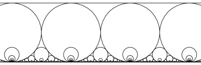
3pt $-1$ [t] at 16 5 $0$ [t] at 100 5 $1$ [t] at 183 5 $2$ [t] at 267 5 $\frac{1}{2}$ [t] at 142 5 $\frac{1}{3}$ [t] at 128 5 $\frac{2}{3}$ [t] at 156 5 $\frac{1}{4}$ [t] at 121 5 $\frac{3}{4}$ [t] at 162.5 5 $\frac{1}{5}$ [t] at 116.75 5 $\frac{2}{5}$ [t] at 133.5 5 $\frac{3}{5}$ [t] at 150 5 $\frac{4}{5}$ [t] at 167 5

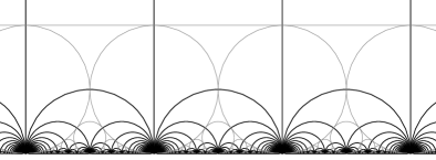
Figure 5: Horocycles $h(p,q)$ with integer parameters $(p,q)\in\mathbb{Z}^{2}$

Figure 6: Ford circles and Farey tessellation

shows the horocycles $h(p,q)$ with integer parameters $(p,q)\in\mathbb{Z}^{2}$. There is an infinite family of such integer horocycles centered at each rational number and at $\infty$. (Only the lowest horocycle centered at $\infty$ is shown to save space.) Integer horocycles $h(p_{1},q_{1})$ and $h(p_{2},q_{2})$ with different centers $\frac{p_{1}}{q_{1}}\not=\frac{p_{2}}{q_{2}}$ do not intersect. This follows from Proposition 6.2, because $p_{1}q_{2}-p_{2}q_{1}$ is a non-zero integer. They touch if and only if $p_{1}q_{2}-p_{2}q_{1}=\pm 1$. This can happen only if both $(p_{1},q_{1})$ and $(p_{2},q_{2})$ are coprime, that is, if $\frac{p_{1}}{q_{1}}$ and $\frac{p_{2}}{q_{2}}$ are reduced fractions representing the respective horocycle centers.

Figure 6 shows the horocycles $h(p,q)$ with integer and coprime parameters $(p,q)$. They are called Ford circles. There is exactly one Ford circle centered at each rational number and at $\infty$. If one connects the ideal centers of tangent Ford circles with geodesics, one obtains the Farey tessellation, which is also shown in the figure. The Farey tessellation is an ideal triangulation of the hyperbolic plane with vertex set $\mathbb{Q}\cup\{\infty\}$. (A thorough treatment can be found in [7].)

We will see that Markov triples correspond to ideal triangulations of the hyperbolic plane (as universal cover of the modular torus), and $(1,1,1)$ corresponds to the Farey tessellation (Sec. 11). The Farey tessellation also comes up when one considers the minima of definite quadratic forms (Sec. 16).

8 Signed distance of a horocycle and a geodesic

For a horocycle $h$ and a geodesic $g$, the signed distance $d(h,g)$ is defined as follows (see Fig. 7):

2pt $h$ [b] at 27 50 $g$ [b] at 108 36 $h$ [b] at 228 73 $g$ [br] at 181 32 $d>0$ [b] <4pt,2pt> at 64 31 $d<0$ [br] <1pt,2pt> at 251 42 $x_{1}$ [t] <2pt, 0pt> at 71 0 $x_{2}$ [t] <2pt, 0pt> at 143 0 $x_{1}$ [t] <2pt, 0pt> at 165 0 $x_{2}$ [t] <2pt, 0pt> at 256 0

Figure 7: The signed distance $d=d(h,g)$ of a horocycle $h$ and a geodesic $g$

• If $h$ and $g$ do not intersect, then $d(h,g)$ is the length of the geodesic segment connecting $h$ and $g$ and orthogonal to both. (This is just the hyperbolic distance between $h$ and $g$.)

• If $h$ and $g$ do intersect, then $d(h,g)$ is the length of that geodesic segment, taken negative.

• If $h$ and $g$ are tangent then $d(h,g)=0$.

• If $g$ ends in the center of $h$ then $d(h,g)=-\infty$.

An equation for the signed distance to a vertical geodesic is particularly easy to derive:

Proposition 8.1 (Signed distance to a vertical geodesic).

Consider a horocycle $h=h(p,q)$ with $q\not=0$ and a vertical geodesic $g$ from $x\in\mathbb{R}$ to $\infty$. Their signed distance is

$$d(h,g)=\log\Big{(}2q^{2}\Big{|}x-\frac{p}{q}\Big{|}\Big{)}.$$ (25)

Proof.

See Fig. 8. ∎

3pt $x$ [t] at 73 10 $\displaystyle\frac{p}{q}$ [t] at 126 10 $d$ [b] at 85 60 $d$ [l] at 126 93 $\displaystyle\frac{1}{q^{2}}$ [l] at 186 71 $2\big{|}x-\frac{p}{q}\big{|}$ [l] at 186 115 $g$ [r] at 74 119 $h$ [tr] at 152 58

Figure 8: Signed distance of horocycle $h=h(p,q)$ and vertical geodesic $g$

Equation (25) suggests a geometric interpretation of Hurwitz’s theorem and the Diophantine approximation version of Markov’s theorem: A fraction $\frac{p}{q}$ satisfies inequality (2) if and only if

$$d\big{(}h(p,q),g\big{)}<-\log\frac{\lambda}{2}\,.$$ (26)

The following section contains a proof of Hurwitz’s theorem based on this observation. An equation for the signed distance to a general geodesic will be presented in Proposition 10.1.

9 Proof of Hurwitz’s theorem

Let $x$ be an irrational number and let $g$ be the vertical geodesic from $x$ to $\infty$. By Proposition 8.1, part (i) of Hurwitz’s theorem is equivalent to the statement:

Infinitely many Ford circles $h$ satisfy

$$d(h,g)<-\log\frac{\sqrt{5}}{2}\,.$$ (27)

This follows from the following lemma. Let us say that the midpoint of an edge of the Farey tessellation is the point where the horocycles centered at its ends meet (see Fig. 6). Accordingly, we say that a geodesic bisects an edge of the Farey tessellation if it passes through the midpoint of the edge (see Fig. 9).

Lemma 9.1.

Suppose a geodesic $g$ crosses an ideal triangle $T$ of the Farey tessellation. If $g$ is one of the three geodesics bisecting two sides of $T$, then

$$d(h,g)=-\log\frac{\sqrt{5}}{2}$$

for all three Ford circles $h$ at the vertices of $T$. Otherwise, inequality (27) holds for at least one of these three Ford circles.

Proof of Lemma 9.1.

This is the simplest case of Propositions 13.2 and 13.4, and easy to prove independently. Note that it is enough to consider the ideal triangle $0$, $1$, $\infty$, and geodesics intersecting its two vertical sides (see Fig. 9). ∎

2pt $\frac{1}{2}-\frac{\sqrt{5}}{2}$ at 5 0 $0$ at 43 0 $\frac{1}{2}$ at 76 0 $1$ at 105 0 $\frac{1}{2}+\frac{\sqrt{5}}{2}=\Phi$ at 152 0 $1$ [l] at 201 72 $\frac{\sqrt{5}}{2}$ [l] at 203 81 $d$ [r] at 73 76 $g_{1}$ [r] at 6 25 $g$ [l] at 142 93 $\frac{\sqrt{5}}{2}$ [l] at 53 52

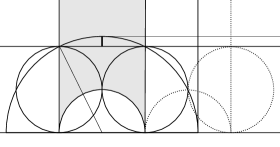
Figure 9: Geodesic $g_{1}$ bisecting the two vertical sides of the triangle $0,1,\infty$, and geodesic $g$ from $\Phi$ to $\infty$

To deduce part (i) of Hurwitz’s theorem, note that since $x$ is irrational, the geodesic $g$ from $x$ to $\infty$ passes through infinitely many triangles of the Farey tessellation. For each of these triangles, at least one of its Ford circles $h$ satisfies (27), by Lemma 9.1. (The geodesic $g$ does not bisect two sides of any Farey triangle. Otherwise, $g$ would bisect two sides of all Farey triangles it enters; see Fig. 9, where the next triangle is shown with dashed lines. This contradicts $g$ ending in the vertex $\infty$ of the Farey tessellation.)

For consecutive triangles that $g$ crosses, the same horocycle may satisfy (27). But this can happen only finitely many times (otherwise $x$ would be rational), and then the geodesic will never again intersect a triangle incident with this horocycle. Hence, infinitely many Ford circles satisfy (27), and this completes the proof of part (i).

To prove part (ii) of Hurwitz’s theorem, we have to show that for

$$x=\Phi\quad\text{and}\quad\epsilon>0,$$

only finitely many Ford circles $h$ satisfy

$$d(h,g)<-\log\frac{\sqrt{5}}{2}-\epsilon,$$ (28)

where $g$ is the geodesic from $\Phi$ to $\infty$.

To this end, let $g_{1}$ be the geodesic from $\Phi=\frac{1}{2}(1+\sqrt{5})$ to $\frac{1}{2}(1-\sqrt{5})$, see Fig. 9. For every Ford circle $h$,

$$d(h,g_{1})\geq-\log\frac{\sqrt{5}}{2}.$$

Indeed, the distance is equal to $-\log\frac{\sqrt{5}}{2}$ for all Ford circles that $g_{1}$ intersects, and positive for all others.

Because the geodesics $g$ and $g_{1}$ converge at the common end $\Phi$, there is a point $P\in g$ such that all Ford circles $h$ intersecting the ray from $P$ to $\Phi$ satisfy

$$|d(g,\Phi)-d(g_{1},\Phi)|<\epsilon,$$

and hence

$$d(g,\Phi)\geq-\log\frac{\sqrt{5}}{2}-\epsilon.$$

On the other hand, the complementary ray of $g$, from $P$ to $\infty$, intersects only finitely many Ford circles. Hence, only finitely many Ford circles satisfy (28), and this completes the proof of part (ii).

Remark 9.2.

The gist of the above proof is deducing Hurwitz’s theorem from the fact that the geodesic $g$ from an irrational number $x$ to $\infty$ crosses infinitely many Farey triangles. A weaker statement follows from the observation that $g$ crosses infinitely many edges. Since each edge has two touching Ford circles at the ends, a crossing geodesic intersects at least one of them. Hence there are infinitely many fractions satisfying (2) with $\lambda=2$. In fact, at least one of any two consecutive continued fraction approximants satisfies this bound. This result is due to Vahlen [59, p. 41] [73]. The converse is due to Legendre [46] and 65 years older: If a fraction satisfies (2) with $\lambda=2$, then it is a continued fraction approximant. A geometric proof using Ford circles is mentioned by Speiser [71] (see Sec. 1).

10 Dictionary: geodesic — indefinite form

We assign a geodesic $g(f)$ to every indefinite binary quadratic form $f$ with real coefficients as follows: To the form $f$ with real coefficients $A$, $B$, $C$ as in (11), we assign the geodesic $g(f)$ that connects the zeros of the polynomial (13). (If $A=0$, one of the zeros is $\infty$, and $g(f)$ is a vertical geodesic.) The map $f\mapsto g(f)$ from the space of indefinite forms to the space of geodesics is

• surjective and many-to-one: $g(f)=g(\tilde{f})\Leftrightarrow\tilde{f}=\mu f$ for some $\mu\in\mathbb{R}^{*}$.

• equivariant with respect to the left $\mathit{GL}_{2}(\mathbb{R})$-actions:

Proposition 10.1.

The signed distance of the horocycle $h(p,q)$ and the geodesic $g(f)$ is

$$d\big{(}h(p,q),g(f)\big{)}=\log\frac{|f(p,q)|}{\sqrt{-\det f}}\,.$$ (29)

Proof.

First, consider the case of horizontal horocycles ($q=0$). If $g(f)$ is a vertical geodesic ($f(p,0)=0$), equation (29) is immediate. Otherwise, note that ${p^{2}\sqrt{-\det f}}/{|f(p,0)|}$ is half the distance between the zeros (14), hence the height of the geodesic.

The general case reduces to this one: For any $A\in\mathit{GL}_{2}(\mathbb{R})$ with $|\det A|=1$ and $A\big{(}\begin{smallmatrix}p\\ q\end{smallmatrix}\big{)}=\big{(}\begin{smallmatrix}\tilde{p}\\ 0\end{smallmatrix}\big{)}$,

$$\begin{split}d\big{(}h(p,q),g(f)\big{)}&=d\big{(}M_{A}h(p,q),M_{A}g(f)\big{)}=d\big{(}h(\tilde{p},0),g(f\circ A^{-1})\big{)}\\ &=\log\frac{|(f\circ A^{-1})(\tilde{p},0)|}{\sqrt{-\det(f\circ A^{-1})}}=\log\frac{|f(p,q)|}{\sqrt{-\det f}}\,.\qed\end{split}$$

Equation (29) suggests a geometric interpretation of the quadratic forms version of Markov’s theorem, and it is easy to prove most of Korkin & Zolotarev’s theorem (just replace inequality (16) with $M(f)<\frac{2}{\sqrt{5}}$) by adapting the proof of Hurwitz’s theorem in Sec. 9. To obtain the complete Markov theorem, more hyperbolic geometry is needed. This this is the subject of the following sections.

11 Decorated ideal triangles

In this and the following section, we review some basic facts from Penner’s theory of decorated Teichmüller spaces [56, 57]. The material of this section, up to and including equation (30) is enough to treat crossing geodesics in Sec. 13. Ptolemy’s relation is needed for the geometric interpretation of Markov’s equation in Sec. 12.

An ideal triangle is a closed region in the hyperbolic plane that is bounded by three geodesics (the sides) connecting three ideal points (the vertices). Ideal triangles have dihedral symmetry, and any two ideal triangles are isometric. That is, for any pair of ideal triangles and any bijection between their vertices, there is a unique hyperbolic isometry that maps one to the other and respects the vertex matching. A decorated ideal triangle is an ideal triangle together with a horocycle at each vertex (Fig. 10).

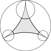
2pt $\alpha_{3}$ [t] at 64 45 $\alpha_{1}$ [bl] at 83 63 $\alpha_{2}$ [br] at 44 63 $c_{3}$ [t] at 64 78 $c_{1}$ [bl] at 33 44 $c_{2}$ [br] <-0.5pt, -1.5pt> at 97 44 $h_{1}$ [t] <1pt,0pt> at 15 51 $h_{2}$ [bl] <0pt, -2pt> at 98 28 $h_{3}$ [r] at 86 102 2pt $\alpha_{3}$ [bl] <-0.5pt,-0.5pt> at 88 52 $\alpha_{1}$ [l] at 131 85 $\alpha_{2}$ [r] at 44 85 $c_{3}$ [t] at 90 118 $c_{1}$ [bl] <-2pt,-1pt> at 56 52 $c_{2}$ [br] <1.5pt, 1.5pt> at 124 42 $0$ [t] at 44 9 $1$ [t] at 131 9 $i$ [br] at 44 96 $1+i$ [bl] at 131 96

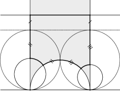
Figure 10: Decorated ideal triangle in the Poincaré disk model (left) and in the half-plane model (right)

Consider a geodesic decorated with two horocycles $h_{1}$, $h_{2}$ at its ends (for example, a side of an ideal triangle). Let the truncated length of the decorated geodesic be defined as the signed distance of the horocycles (Sec. 6),

$$\alpha=d(h_{1},h_{2}),$$

and let its weight be defined as

$$a=e^{\alpha/2}.$$

(We will often use Greek letters for truncated lengths and Latin letters for weights. The weights are usually called $\lambda$-lengths.)

Any triple $(\alpha_{1},\alpha_{2},\alpha_{3})\in\mathbb{R}^{3}$ of truncated lengths, or, equivalently, any triple $(a_{1},a_{2},a_{3})\in\mathbb{R}_{>0}^{3}$ of weights, determines a unique decorated ideal triangle up to isometry.

Consider a decorated ideal triangle with truncated lengths $\alpha_{k}$ and weights $a_{k}$. Its horocycles intersect the triangle in three finite arcs. Denote their hyperbolic lengths by $c_{k}$ (see Fig. 10). The truncated side lengths determine the horocyclic arc lengths, and vice versa, via the relation

$$c_{k}=\frac{a_{k}}{a_{i}a_{j}}=e^{\frac{1}{2}(-\alpha_{i}-\alpha_{j}+\alpha_{k})},$$ (30)

where $(i,j,k)$ is a permutation of $(1,2,3)$. (For a proof, contemplate Fig. 10.)

Now consider a decorated ideal quadrilateral as shown in Fig. 12.

2pt $a$ [t] at 66 46 $b$ [l] at 107 59 $c$ [bl] at 94 78 $d$ [br] at 45 66 $e$ [br] at 71 60 $f$ [tr] <0pt,4pt> at 89 55

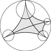
Figure 11: Ptolemy relation

2pt $a$ [l] at 63 55 $a^{\prime}$ [b] at 76 67 $b$ [tl] at 82 54 $b$ [br] at 43 72 $c$ [bl] at 84 88 $c$ [tr] at 42 41

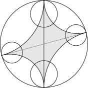
Figure 12: Triangulations $T$ and $T^{\prime}$ of a punctured torus

It can be decomposed into two decorated ideal triangles in two ways. The six weights $a$, $b$, $c$, $d$, $e$, $f$ are related by the Ptolemy relation

$$ef=ac+bd.$$ (31)

It is straightforward to derive this equation using the relations (30).

12 Triangulations of the modular torus and Markov’s equation

In this section, we review Penner’s [56, 57] geometric interpretation of Markov’s equation (4), which is summarized in Prop. 12.1. The involutions $\sigma_{k}$ were defined in Sec. 2, see equation (7). The modular torus is the orbit space

$$M=H^{2}/G,$$

where $G$ is the group of orientation preserving hyperbolic isometries generated by

$$A(z)=\frac{z-1}{-z+2},\qquad B(z)=\frac{z+1}{z+2}.$$ (32)

Figure 13 shows a fundamental domain.

2pt $-1$ [t] at 36 8 $0$ [t] at 94 8 $1$ [t] at 152 8 $B$ [bl] at 65 97 $A$ [br] at 122 97

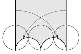
Figure 13: The modular torus

The group $G$ is the commutator subgroup of the modular group $\mathit{PSL}_{2}(\mathbb{Z})$, and the only subgroup of $\mathit{PSL}_{2}(\mathbb{Z})$ that has a once punctured torus as orbit space. It is a normal subgroup of $\mathit{PSL}_{2}(\mathbb{Z})$ with index six, and the quotient group $\mathit{PSL}_{2}(\mathbb{Z})/G$ is the group of orientation preserving isometries of the modular torus $M$. It is also symmetric with respect to six reflections, so the isometry group has in total twelve elements.

Proposition 12.1 (Markov triples and ideal triangulations).

(i) A triple $\tau=(a,b,c)$ of positive integers is a Markov triple if and only if there is an ideal triangulation of the decorated modular torus whose three edges have the weights $a$, $b$, and $c$. This triangulation is unique up to the $12$-fold symmetry of the modular torus.

(ii) If $T$ is an ideal triangulation of the decorated modular torus with edge weights $\tau=(a,b,c)$, and if $T^{\prime}$ is an ideal triangulation obtained from $T$ by performing a single edge flip, then the edge weights of $T^{\prime}$ are $\tau^{\prime}=\sigma_{k}\tau$, with $k\in\{1,2,3\}$ depending on which edge was flipped.

To understand the logical connections, it makes sense to consider not only the modular torus but arbitrary once punctured hyperbolic tori.

A once punctured hyperbolic torus is a torus with one point removed, equipped with a complete metric of constant curvature $-1$ and finite volume. For example, one obtains a once punctured hyperbolic torus by gluing two congruent decorated ideal triangles along their edges in such a way that the horocycles fit together. Conversely, every ideal triangulation of a hyperbolic torus with one puncture decomposes it into two ideal triangles.

A decorated once punctured hyperbolic torus is a once punctured hyperbolic torus together with a choice of horocycle at the cusp. Thus, a triple of weights $(a,b,c)\in\mathbb{R}_{>0}^{3}$ determines a decorated once punctured hyperbolic torus up to isometry, together with an ideal triangulation. Conversely, a decorated once punctured hyperbolic torus together with an ideal triangulation determines such a triple of edge weights.

Consider a decorated once punctured hyperbolic torus with an ideal triangulation $T$ with edge weights $(a,b,c)\in\mathbb{R}_{>0}^{3}$. By equation (30), the total length of the horocycle is

$$\ell=2\big{(}\frac{a}{bc}+\frac{b}{ca}+\frac{c}{ab}\big{)}.$$

This equation is equivalent to

$$a^{2}+b^{2}+c^{2}=\frac{\ell}{2}\,abc.$$

Thus, the weights satisfy Markov’s equation (4) (not considered as a Diophantine equation) if and only if the horocycle has length $\ell=6$. From now on, we assume that this is the case: We decorate all once punctured hyperbolic tori with the horocycle of length $6$.

Let $T^{\prime}$ be the ideal triangulation obtained from $T$ by flipping the edge with weight $a$, i.e., by replacing this edge with the other diagonal in the ideal quadrilateral formed by the other edges (see Fig. 12). By equation (6) and Ptolemy’s relation (31), the edge weights of $T^{\prime}$ are $(a^{\prime},b,c)=\sigma_{1}(a,b,c)$. Of course, one obtains analogous equations if a different edge is flipped.

The modular torus $M$, decorated with a horocycle of length $6$, is obtained by gluing two decorated ideal triangles with weights $(1,1,1)$. Lifting this triangulation and decoration to the hyperbolic plane, one obtains the Farey tessellation with Ford circles (Fig. 6). This implies that for every Markov triple $(a,b,c)$ there is an ideal triangulation of the decorated modular torus with edge weights $a$, $b$, $c$. To see this, follow the path in the Markov tree leading from $(1,1,1)$ to $(a,b,c)$ and perform the corresponding edge flips on the projected Farey tessellation.

On the other hand, the flip graph of a complete hyperbolic surface with punctures is also connected [35] [55, p. 36ff]. The flip graph has the ideal triangulations as vertices, and edges connect triangulations related by a single edge flip. (Since we are only interested in a once punctured torus, invoking this general theorem is somewhat of an overkill.) This implies the converse statement: If $a$, $b$, $c$ are the weights of an ideal triangulation of the modular torus, then $(a,b,c)$ is a Markov triple.

Note that there is only one ideal triangulation of the modular torus with weights $(1,1,1)$, i.e., the triangulation that lifts to the Farey tessellation. The symmetries of the modular torus permute its edges. Since the Markov tree and the flip graph are isomorphic, this implies that two triangulations with the same weights are related by an isometry of the modular torus. Altogether, one obtains Proposition 12.1.

13 Geodesics crossing a decorated ideal triangle

For the proof of Markov’s theorem in Sec. 15, we need to know how far a geodesic crossing a decorated ideal triangle can stay away from the horocycles at the vertices. To prove Hurwitz’s theorem (see Sec. 9), it was enough to consider a triangle decorated with pairwise tangent horocycles. In this section, we consider the general case, more precisely, the following geometric optimization problem:

Problem 13.1.

Given a decorated ideal triangle with two sides, say $a_{1}$ and $a_{2}$, designated as “legs”, and the third side, say $a_{3}$, designated as “base”. Find, among all geodesics intersecting both legs, a geodesic that maximizes the minimum of signed distances to the three horocycles at the vertices.

It makes sense to consider the corresponding optimization problem for euclidean triangles: Which straight line crossing two given legs has the largest distance to the vertices? The answer depends on whether or not an angle at the base is obtuse. For decorated ideal triangles, the situation is completely analogous. We say that a geodesic bisects a side of a decorated ideal triangle if it intersects the side in the point at equal distance to the two horocycles at the ends of the side.

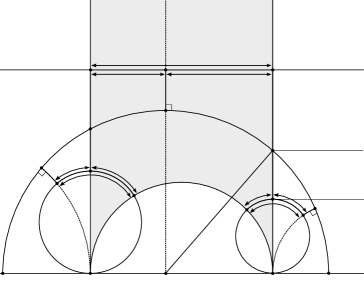
2pt $v_{2}$ [t] at 198 9 $v_{1}$ [t] at 67 9 $v_{3}=\infty$ [l] at 130 200 $a_{1}$ [l] at 197 120 $a_{2}$ [r] at 66 130 $a_{3}$ [t] at 133 74 $h_{2}$ [br] at 220 21 $h_{1}$ [bl] at 32 29 $h_{3}$ [b] at 32 156 $g$ [r] at 11 50 $P_{2}$ [bl] at 228 51 $P_{1}$ [br] at 30 83 $P_{3}$ [tl] <-2pt,0pt> at 121 126 $c_{2}$ [br] at 186 63 $c_{1}$ [bl] at 84 81 $c_{3}$ [b] at 129 159 $s_{2}$ [t] at 93 152 $s_{2}$ [br] at 54 82 $s_{1}$ [t] at 156 152 $s_{1}$ [bl] <-1pt, -2pt> at 212 61 $s_{3}$ [tr] at 65 79 $s_{3}$ [tl] at 199 58 $x_{1}$ [t] <1pt,0pt> at 2 9 $x_{0}$ [t] <1pt,0pt> at 120 9 $x_{2}$ [t] <1pt,0pt> at 236.5 9 $r$ [br] at 145 38 $\,1$ [l] at 261 156 $\frac{1}{a_{1}}$ [l] at 261 97 $\frac{1}{a_{1}^{2}}$ [l] at 261 61 2pt $v_{2}$ [t] at 158 9 $v_{1}$ [t] at 68 9 $v_{3}=\infty$ [t] at 111 204 $h_{2}$ [r] at 148 18 $h_{1}$ [l] at 27 33 $h_{3}$ [b] at 17 156 $g$ [b] at 13 119 $P_{2}$ [l] at 169 23 $P_{1}$ [b] at 82 123 $P_{3}$ [t] at 53 125 $a_{1}$ [l] at 157 96 $a_{2}$ [br] at 67 129 $a_{3}$ [t] at 124 52 $c_{3}$ [b] at 106 159 $s_{2}$ [b] at 60 159 $s_{1}$ [t] at 98 151 $c_{1}$ [bl] at 102 88 $s_{3}$ [tr] at 99 84 $s_{2}$ [t] at 70.5 97 $c_{2}$ [b] at 153 29 $s_{1}$ [b] at 163 27 $s_{3}$ [t] at 159.5 26

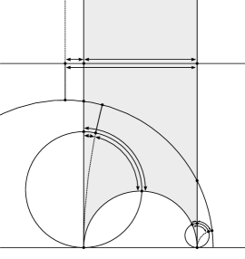
Figure 14: Decorated ideal triangle (shaded) and geodesic $g$ through the midpoints of sides $a_{1}$ and $a_{2}$. Left: Inequalities (33) are strictly satisfied and $P_{3}$ lies strictly between $P_{1}$ and $P_{2}$. (The height marks on the right margin belong to the proof of Proposition 13.4.) Right: $a_{1}^{2}>a_{2}^{2}+a_{3}^{2}$ and $P_{1}$ lies strictly between $P_{3}$ and $P_{2}$.

Proposition 13.2.

Consider a decorated ideal triangle with horocycles $h_{1}$, $h_{2}$, $h_{3}$, and let $a_{1}$, $a_{2}$, $a_{3}$ denote both the sides and their weights (see Fig. 14 for notation).

(i) If

$$a_{1}^{2}\leq a_{2}^{2}+a_{3}^{2}\quad\text{and}\quad a_{2}^{2}\leq a_{1}^{2}+a_{3}^{2},$$ (33)

then the geodesic $g$ bisecting the sides $a_{1}$ and $a_{2}$ is the unique solution of Problem 13.1.

(ii) If, for $(j,k)\in\{(1,2),(2,1)\}$,

$$a_{j}^{2}\geq a_{k}^{2}+a_{3}^{2},$$ (34)

then the perpendicular bisector $g^{\prime}$ of side $a_{k}$ is the unique solution of Problem 13.1. In this case, the minimal distance is attained for $h_{j}$ and $h_{3}$,

$$d(h_{j},g^{\prime})=d(h_{3},g^{\prime})=\frac{\alpha_{k}}{2}\leq d(h_{k},g^{\prime}).$$ (35)

In the proof of Markov’s theorem (Sec. 15), the base $a_{3}$ will always be a largest side, so only part (i) of Proposition 13.2 is needed. We will also need some equations for the geodesic bisecting two sides, which we collect in Proposition 13.4.

Proof of Proposition 13.2.

1. The geodesic $g$ has equal distance from all three horocycles. Indeed, because of the $180^{\circ}$ rotational symmetry around the intersection point, any geodesic bisecting a side has equal distance from the two horocycles at the ends.

2. For $k\in\{1,2,3\}$ let $P_{k}$ be the foot of the perpendicular from vertex $v_{k}$ to the geodesic $g$ bisecting $a_{1}$ and $a_{2}$ (see Fig. 14). If $P_{3}$ lies strictly between $P_{1}$ and $P_{2}$ (as in Fig. 14, left), then $g$ is the unique solution of Problem 13.1. Any other geodesic crossing $a_{1}$ and $a_{2}$ also crosses at least one of the rays from $P_{k}$ to $v_{k}$, and is therefore closer to at least one of the horocycles.

3. If $P_{1}$ lies strictly between $P_{3}$ and $P_{2}$ (as in Fig. 14, right) then the unique solution of Problem 13.1 is the perpendicular bisector of $a_{2}$. Its signed distance to the horocycles $h_{1}$ and $h_{3}$ is half the truncated length of side $a_{2}$. Any other geodesic crossing $a_{2}$ is closer to at least one of its horocycles. The signed distance of $g$ and the horocycle $h_{1}$ is larger. The case when $P_{1}$ lies strictly between $P_{3}$ and $P_{2}$ is treated in the same way.

5. If $P_{2}=P_{3}$ (or $P_{1}=P_{3}$) then the geodesic $g$ with equal distance to all horocycles is simultaneously the perpendicular bisector of side $a_{2}$ (or $a_{1}$).

6. It remains to show that the order of the points $P_{k}$ on $g$ depends on whether the weights satisfy the inequalities (33) or one of the inequalities (34). To this end, let $s_{1}$ be the distance from the side $a_{1}$ to the ray $P_{3}v_{3}$, measured along the horocycle $h_{3}$ in the direction from $a_{1}$ to $a_{2}$. Similarly, let $s_{2}$ be the distance from the side $a_{2}$ to the ray $P_{3}v_{3}$, measured along the horocycle $h_{3}$ in the direction from $a_{2}$ to $a_{1}$. So $s_{1}$ and $s_{2}$ are both positive if and only if $P_{3}$ lies strictly between $P_{1}$ and $P_{2}$. But if, for example, $P_{1}$ lies between $P_{3}$ and $P_{2}$ as in Fig. 14, right, then $s_{2}<0$. By symmetry, $s_{1}$ is also the distance from $a_{1}$ to $P_{2}v_{2}$, measured along $h_{2}$ in the direction away from $a_{3}$. Similarly, $s_{2}$ is also the distance between $a_{2}$ and $P_{1}v_{1}$ along $h_{1}$. Finally, let $s_{3}>0$ be the equal distances between $a_{3}$ and $P_{1}v_{1}$ along $h_{1}$, and between $a_{3}$ and $P_{2}v_{2}$ along $h_{2}$. Now

$$c_{1}=-s_{2}+s_{3},\quad c_{2}=-s_{1}+s_{3},\quad c_{3}=s_{1}+s_{2}$$

implies

$$2s_{1}=c_{1}-c_{2}+c_{3}\overset{\eqref{eq:c}}{=}\frac{a_{1}}{a_{2}a_{3}}-\frac{a_{2}}{a_{3}a_{1}}+\frac{a_{3}}{a_{1}a_{2}}=\frac{a_{1}^{2}-a_{2}^{2}+a_{3}^{2}}{a_{1}a_{2}a_{3}}$$ (36)

and similarly

$$2s_{2}=\frac{-a_{1}^{2}+a_{2}^{2}+a_{3}^{2}}{a_{1}a_{2}a_{3}}.$$

Hence, $P_{3}$ lies in the closed interval between $P_{1}$ and $P_{2}$ if and only if inequalities (33) are satisfied. The other cases are treated similarly. ∎

Remark 13.3.

The above proof of Proposition 13.2 is nicely intuitive. A more analytic proof may be obtained as follows. First, show that for all geodesics intersecting $a_{1}$ and $a_{2}$, the signed distances $u_{1}$, $u_{2}$, $u_{3}$ to the horocycles satisfy the equation

$$(c_{1}u_{1}+c_{2}u_{2}+c_{3}u_{3})^{2}-4c_{1}c_{2}u_{1}u_{2}-4=0$$ (37)

It makes sense to consider the special case $a_{1}=a_{2}=a_{3}=1$ first, because the general equation (37) can easily be derived from the simpler one. Then consider the necessary conditions for a local maximum of $\min(u_{1},u_{2},u_{3})$ under the constraint (37): If a maximum is attained with $u_{1}=u_{2}=u_{3}$, then the three partial derivatives of the left hand side of (37) are all $\geq 0$ or all $\leq 0$. If a maximum is attained with $u_{1}=u_{2}<u_{3}$, then this sign condition holds for the first two derivatives, and similarly for the other cases.

Proposition 13.4.

Let $g$ be the geodesic bisecting sides $a_{1}$ and $a_{2}$ of a decorated ideal triangle as shown in Fig. 14. (Inequalities (33) may hold or not.) Then the common signed distance of $g$ and the horocycles is

$$d(h_{1},g)=d(h_{2},g)=d(h_{3},g)=-\log r,$$

where

$$r=\sqrt{\frac{\delta^{2}}{4}-\frac{1}{a_{3}^{2}}},$$ (38)

and $\delta$ is the sum of the lengths of the horocyclic arcs,

$$\delta=c_{1}+c_{2}+c_{3}=\frac{a_{1}}{a_{2}a_{3}}+\frac{a_{2}}{a_{3}a_{1}}+\frac{a_{3}}{a_{1}a_{2}}.$$ (39)

Moreover, suppose the vertices are

$$v_{1}<v_{2},\quad v_{3}=\infty,$$ (40)

and the horocycle $h_{3}$ has height $1$. Then the ends $x_{1,2}$ of $g$ are

$$x_{1,2}=x_{0}\pm r,$$ (41)

where

$$x_{0}=v_{2}+\frac{a_{2}}{a_{3}a_{1}}-\frac{\delta}{2}$$ (42)

Proof.

Assuming (40) and $h_{3}=h(1,0)$, let $x_{0}=v_{2}-s_{1}$. Then the proposition follows from (36), some easy hyperbolic geometry, Pythagoras’ theorem, and simple algebra (see Fig. 14). ∎

14 Simple closed geodesics and ideal arcs

In this section, we collect some topological facts about simple closed geodesics and ideal arcs that we will use in the proof of Markov’s theorem (Sec. 15). They are probably well known, but we indicate proofs for the reader’s convenience.

An ideal arc in a complete hyperbolic surface with cusps is a simple geodesic connecting two punctures or a puncture with itself. The edges of an ideal triangulation are ideal arcs, and every ideal arc occurs in an ideal triangulation. (In fact, ideal triangulations are exactly the maximal sets of non-intersecting ideal arcs.) Here, we are only interested in a once punctured hyperbolic torus. In this case, every ideal triangulation containing a fixed ideal arc can be obtained from any other such triangulation by repeatedly flipping the remaining two edges. Ideal arcs play an important role in the following section because they are in one-to-one correspondence with the simple closed geodesics (Proposition 14.1), and the simple closed geodesics are the geodesics that stay farthest away from the puncture (Proposition 15.1).

Proposition 14.1.

Consider a fixed once punctured hyperbolic torus.

(i) For every ideal arc $c$, there is a unique simple closed geodesic $g$ that does not intersect $c$.

(ii) Every other geodesic not intersecting $c$ has either two ends in the puncture, or one end in the puncture and the other end approaching the closed geodesic $g$.

(iii) If $a$, $b$, $c$ are the edges of an ideal triangulation $T$, then the simple closed geodesic $g$ that does not intersect $c$ intersects each of the two triangles of $T$ in a geodesic segment bisecting the edges $a$ and $b$.

(iv) For every simple closed geodesic $g$, there is a unique ideal arc $c$ that does not intersect $g$.

Remark 14.2.

Speaking of edge midpoints implies an (arbitrary) choice of a horocycle at the cusp. In fact, the edge midpoints of a triangulated once punctured torus are distinguished without any choice of triangulation. They are the three fixed points of an orientation preserving isometric involution. Every ideal arc passes through one of these points.

Proof.

(i) Cut the torus along the ideal arc $c$. The result is a hyperbolic cylinder as shown in Fig. 15 (left).

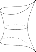
2pt $c$ [t] at 29 73 $g$ [t] at 29 44 $c$ [b] at 29 13 2pt $g$ [t] at 30 69 $c$ [t] at 30 40 $g$ [b] at 30 0

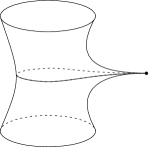
Figure 15: Cutting a punctured torus along an ideal arc (left) and along a simple closed geodesic (right).

Both boundary curves are complete geodesics with both ends in the cusp, which is now split in two. There is up to orientation a unique non-trivial free homotopy class that contains simple curves, and this class contains a unique simple closed geodesic.

(ii) Consider the universal cover of the cylinder in the hyperbolic plane.

(iii) An ideal triangulation of a once punctured torus is symmetric with respect to a $180^{\circ}$ rotation around the edge midpoints. (This is the involution mentioned in Remark 14.2.) It swaps the geodesic segments bisecting edges $a$ and $b$ in the two ideal triangles, so they connect smoothly. Hence they form a simple closed geodesic, which does not intersect $c$.

(iv) Cut the torus along the simple closed geodesic $g$. The result is a cylinder with a cusp and two geodesic boundary circles, as shown in Fig. 15 (right). Fill the puncture and take it as base point for the homotopy group. There is up to orientation a unique non-trivial homotopy class containing simple closed curves and this class contains a unique ideal arc. ∎

15 Proof of Markov’s theorem

In this section, we put the pieces together to prove both versions of Markov’s theorem. The quadratic forms version follows from Proposition 15.1. The Diophantine approximation version follows from Proposition 15.1 together with Proposition 15.2.

Two geodesics in the hyperbolic plane are $\mathit{GL}_{2}(\mathbb{Z})$-related if, for some $A\in\mathit{GL}_{2}(\mathbb{Z})$, the hyperbolic isometry $M_{A}$ maps one to the other.

Proposition 15.1.

Let $g$ be a complete geodesic in the hyperbolic plane, and let $\pi(g)$ be its projection to the modular torus. Then the following three statements are equivalent:

1. $\pi(g)$ is a simple closed geodesic.

2. There is a Markov triple $(a,b,c)$ so that for one (hence any) choice of integers $p_{1}$, $p_{2}$ satisfying (8), the geodesic $g$ is $\mathit{GL}_{2}(\mathbb{Z})$-related to the geodesic ending in $x_{0}\pm r$ with $x_{0}$ and $r$ defined by (18) and (19).

3. The greatest lower bound for the signed distances of $g$ and a Ford circle is greater than $-\log\frac{3}{2}$.

If $g$ satisfies one (hence all) of the statements (a), (b), (c), then

1. the minimal signed distance of $g$ and a Ford circle is $-\log r$,

2. among all Markov triples $(a,b,c)$ that verify (b), there is a unique sorted Markov triple.

Proof.

“$\textit{(a)}\Rightarrow\textit{(b)}$”: If $\pi(g)$ is a simple closed geodesic, then there is a unique ideal arc $c$ not intersecting $\pi(g)$ (Proposition 14.1 (iv)). Pick an ideal triangulation $T$ of the modular torus that contains $c$, and let $a$ and $b$ be the other edges. By Proposition 12.1, $(a,b,c)$ is a Markov triple. (We use the same letters to denote both ideal arcs and their weights.) The geodesic $\pi(g)$ intersects each of the two triangles of $T$ in a geodesic segment bisecting the edges $a$ and $b$ (Proposition 14.1 (iii)).

Now let $p_{1}$, $p_{2}$ be integers satisfying (8) and consider the decorated ideal triangle in $H^{2}$ with vertices

$$v_{1}=\frac{p_{1}}{b},\quad v_{2}=\frac{p_{2}}{a},\quad v_{3}=\infty,$$ (43)

and their respective Ford circles

$$h_{1}=h(p_{1},b),\quad h_{2}=h(p_{2},a),\quad h_{3}=h(1,0).$$ (44)

Such integers $p_{1}$, $p_{2}$ exist because the numbers $a$, $b$, $c$ of a Markov triple are pairwise coprime. Moreover, this implies that the fractions in (43) are reduced, and $v_{1}$ and $v_{2}$ are determined up to addition of a common integer. By Proposition 6.2, this decorated ideal triangle has edge weights

$$a_{1}=a,\quad a_{2}=b,\quad a_{3}=c$$ (45)

(see Fig. 14 for notation).

Conversely, every ideal triangle $\tilde{v}_{1}\tilde{v}_{2}\tilde{v}_{3}$ with $\tilde{v}_{3}=\infty$ and rational $\tilde{v}_{1}$, $\tilde{v}_{2}$, that is decorated with the respective Ford circles, has weights (45), and satisfies $\tilde{v}_{1}<\tilde{v}_{2}$ is obtained this way. (To get the triangles with $\tilde{v}_{1}>\tilde{v}_{2}$, change $c$ to $-c$ in equation (8).) This implies that any lift of a triangle of $T$ to the hyperbolic plane is $\mathit{GL}_{2}(\mathbb{Z})$-related to $v_{1}v_{2}v_{3}$. Use Proposition 13.4 with $\delta=3$ to deduce that $g$ is $\mathit{GL}_{2}(\mathbb{Z})$-related to the geodesic ending in $x_{0}\pm r$.

“$\textit{(b)}\Rightarrow\textit{(d)}$”: Let $\hat{T}$ be the lift of the triangulation $T$ to $H^{2}$. The geodesic $g$ crosses an infinite strip of triangles of $\hat{T}$. By Proposition 13.4, the signed distance of $g$ and any Ford circle centered at a vertex incident with this strip is $-\log r$. We claim that the signed distance to any other Ford circle is larger. To see this, consider a vertex $v\in\mathbb{Q}\cup\{\infty\}$ that is not incident with the triangle strip, and let $\rho$ be a geodesic ray from $v$ to a point $p\in g$. Note that the projected ray $\pi(\rho)$ intersects $\pi(g)$ at least once before it ends in $\pi(p)$, and that the signed distance to the first intersection is at least $-\log r$.

“$\textit{(b)}\land\textit{(d)}\Rightarrow\textit{(c)}$”: This follows directly from $r=\sqrt{\frac{9}{4}-\frac{1}{c^{2}}}<\frac{3}{2}$.

“$\textit{(c)}\Rightarrow\textit{(a)}$”: We will show the contrapositive: If the geodesic $g$ does not project to a simple closed geodesic, then there is a Ford circle with signed distance smaller than $-\log\frac{3}{2}+\epsilon$, for every $\epsilon>0$.

There is nothing to show if at least one end of $g$ is in $\mathbb{Q}\cup\{\infty\}$ because then the Ford circle at this end has signed distance $-\infty$. So assume $g$ does not project to a simple closed geodesic and both ends of $g$ are irrational.

We will recursively define a sequence $(T_{n})_{n\geq 0}$ of ideal triangulations of the modular torus, with edges labeled $a_{n}$, $b_{n}$, $c_{n}$, such that the following holds:

1. The geodesic $\pi(g)$ has at least one pair of consecutive intersections with the edges $a_{n}$, $b_{n}$.

2. The edge weights, which we also denote by $a_{n}$, $b_{n}$, $c_{n}$, satisfy

   $$a_{n}\leq b_{n}\leq c_{n},$$

   so that $(a_{n},b_{n},c_{n})$ is a sorted Markov triple.

3. $c_{n+1}>c_{n}$

This proves the claim, because Propositions 13.2 and 13.4 imply that for each $n$, there is a horocycle with signed distance to $g$ less than $-\frac{1}{2}\log\big{(}\frac{9}{4}-\frac{1}{c_{n}^{2}}\big{)},$ which tends to $-\log\frac{3}{2}$ from above as $n\rightarrow\infty$.

To define the sequence $(T_{n})$, let $T_{0}$ be the triangulation with edge weights $(1,1,1)$, with edges labeled so that (1) holds.

Suppose the triangulation $T_{n}$ with labeled edges is already defined for some $n\geq 0$. Define the labeled triangulation $T_{n+1}$ as follows. Since $\pi(g)$ is not a simple closed geodesic, it intersects all three edges. Because $g$ has an irrational end (in fact, both ends are assumed to be irrational), there are infinitely many edge intersections. Hence, there is pair of intersections with $a_{n}$ and $b_{n}$ next to an intersection with $c_{n}$. If the sequence of intersections is $a_{n}b_{n}c_{n}$, let $T_{n+1}$ be the triangulation with edges

$$(a_{n+1},b_{n+1},c_{n+1})=(a_{n},c_{n},b_{n}^{\prime}),$$

and if the sequence is $b_{n}a_{n}c_{n}$, let $T_{n+1}$ be the triangulation with

$$(a_{n+1},b_{n+1},c_{n+1})=(b_{n},c_{n},a^{\prime}_{n}),$$

where $a_{n}^{\prime}$ and $b_{n}^{\prime}$ are the ideal arcs obtained by flipping the edges $a_{n}$ or $b_{n}$ in $T_{n}$, respectively. By induction on $n$, one sees that (1), (2), (3) are satisfied for all $n\geq 0$.

“$\textit{(a)}\land\textit{(b)}\Rightarrow\textit{(e)}$”: The Markov triples $(a,b,c)$ verifying (b) are precisely the triples of edge weights of ideal triangulations containing the ideal arc $c$ not intersecting $\pi(g)$. The triangulations containing the ideal arc $c$ form a doubly infinite sequence in which neighbors are related by a single edge flip fixing $c$. In this sequence, there is a unique triangulation for which the weight $c$ is largest. ∎

Proposition 15.2.

Let $g$ be a complete geodesic in the hyperbolic plane, and let $X\subset\mathbb{R}\setminus\mathbb{Q}$ be the set of ends of lifts of simple closed geodesics in the modular torus. Then the following two statements are equivalent:

1. The ends of $g$ are contained in $\mathbb{Q}\cup\{\infty\}\cup X$.

2. For some $M>-\log\frac{3}{2}$ there are only finitely many (possibly zero) Ford circles $h$ with signed distance $d(g,h)<M$.

Proof.

“$\textit{(i)}\Rightarrow\textit{(ii)}$”: Consider the ends $x_{k}$ of $g$, $k\in\{1,2\}$.

If $x_{k}\in\mathbb{Q}\cup\{\infty\}$, then $g$ contains a ray $\rho_{k}$ that is contained inside the Ford circle at $x_{k}$. In this case, let $M_{k}=0$.

If $x_{k}\in X$, then $x_{k}$ is also the end of a geodesic $\tilde{g}$ that projects to a simple closed geodesic in the modular torus. By Proposition 15.1, $\inf d(h,\tilde{g})>-\log\frac{3}{2}$, where the infimum is taken over all Ford circles $h$. Since $g$ and $\tilde{g}$ converge at $x_{k}$, there is a constant $M_{k}>-\log\frac{3}{2}$ and a ray $\rho_{k}$ contained in $g$ and ending in $x_{k}$ such that $d(h,\rho_{k})>M_{k}$ for all Ford circles $h$.

The part of $g$ not contained in $\rho_{1}$ or $\rho_{2}$ is empty or of finite length, so it can intersect the interiors of at most finitely many Ford circles. This implies (ii) with $M=\min(M_{1},M_{2})$.

“$\textit{(ii)}\Rightarrow\textit{(i)}$”: To show the contrapositive, assume (i) is false: At least one end of $g$ is irrational but not the end of a lift of a simple closed geodesic in the modular torus. This implies that the projection $\pi(g)$ intersects every ideal arc in the modular torus infinitely many times. Adapt the argument for the implication “$\text{(c)}\Rightarrow\text{(a)}$” in the proof of Proposition 15.1 to show that there is a sequence of horocycles $(h_{n})$ and an increasing sequence of Markov numbers $(c_{n})$ such that $d(g,h_{n})<-\frac{1}{2}\log\big{(}\frac{9}{4}-\frac{1}{c_{n}^{2}}\big{)}$. This implies that (ii) is false. ∎

16 Dictionary: point — definite form. Spectrum, classification of definite forms, and the Farey tessellation revisited

This section is about the hyperbolic geometry of definite binary quadratic forms. Its purpose is to complete the dictionary and provide a broader perspective. This section is not needed for the proof of Markov’s theorem.

If the binary quadratic form (11) with real coefficients is positive or negative definite, then the polynomial $f(x,1)$ has two complex conjugate roots. Let $z(f)$ denote the root in the upper half-plane, i.e.,

$$z(f)=\frac{-B+i\sqrt{\det f}}{A}\,.$$

This defines a map $f\mapsto z(f)$ from the space of definite forms to the hyperbolic plane $H^{2}$. It is surjective and many-to-one (any non-zero multiple of a form is mapped to the same point) and equivariant with respect to the left $\mathit{GL}_{2}(\mathbb{R})$-actions.

The signed distance of a horocycle and a point in the hyperbolic plane is defined in the obvious way (positive for points outside, negative for points inside the horocycle). One obtains the following proposition in the same way as the corresponding statement about geodesics (Proposition 10.1):

Proposition 16.1.

The signed distance of the horocycle $h(p,q)$ and the point $z(f)\in H^{2}$ is

$$d\big{(}h(p,q),z(f)\big{)}=\log\frac{|f(p,q)|}{\sqrt{\det f}}\,.$$ (46)

This provides a geometric explanation for the different behavior of definite binary quadratic forms with respect to their minima on $\mathbb{Z}^{2}$:

For all definite forms $f$, the infimum (15) is attained for some $(p,q)\in\mathbb{Z}^{2}$ and satisfies $M(f)\leq\frac{2}{\sqrt{3}}$. All forms equivalent to $p^{2}-pq+q^{2}$, and only those, satisfy $M(f)=\frac{2}{\sqrt{3}}$. But for every positive number $m<\frac{2}{\sqrt{3}}$, there are infinitely many equivalence classes of definite forms with $M(f)=m$.

Algorithms to determine the minimum $M(f)$ of a definite quadratic form $f$ are based on the reduction theory for quadratic forms. (The theory of equivalence and reduction of binary quadratic forms is usually developed for integer forms, but much of it carries over to forms with real coefficients.) The reduction algorithm described by Conway [15] has a particularly nice geometric interpretation based on the following observation:

For a point in the hyperbolic plane, the three nearest Ford circles (in the sense of signed distance) are the Ford circles at the vertices of the Farey triangle containing the point. (If the point lies on an edge of the Farey tessellation, the third nearest Ford circle is not unique.)

Acknowledgement.

I would like to thank Oliver Pretzel, who gave me a first glimpse of this subject some 25 years ago, and Alexander Veselov, who made me look again. Last but not least, I would like to thank the anonymous referees for their insightful comments.

This research was supported by DFG SFB/TR 109 “Discretization in Geometry and Dynamics”.

Boris Springborn Technische Universität Berlin Institut für Mathematik, MA 8-3 Str. des 17. Juni 136 10623 Berlin, Germany boris.springborn@tu-berlin.de

References

- [1] R. Abe and I. R. Aitchison. Geometry and Markoff’s spectrum for , I. Trans. Amer. Math. Soc., 365(11):6065–6102, 2013.
- [2] M. Aigner. Markov’s theorem and 100 years of the uniqueness conjecture. Springer, Cham, 2013.
- [3] V. I. Arnold. Higher-dimensional continued fractions. Regul. Chaotic Dyn., 3(3):10–17, 1998.
- [4] V. I. Arnold. Tsepnye drobi (Continued fractions, in Russian). MTsNMO, Moscow, 2001.
- [5] A. F. Beardon, J. Lehner, and M. Sheingorn. Closed geodesics on a Riemann surface with application to the Markov spectrum. Trans. Amer. Math. Soc., 295(2):635–647, 1986.
- [6] E. Bombieri. Continued fractions and the Markoff tree. Expo. Math., 25(3):187–213, 2007.
- [7] F. Bonahon. Low-dimensional geometry, volume 49 of Student Mathematical Library. American Mathematical Society, Providence, RI; Institute for Advanced Study (IAS), Princeton, NJ, 2009.
- [8] B. H. Bowditch. A proof of McShane’s identity via Markoff triples. Bull. London Math. Soc., 28(1):73–78, 1996.
- [9] B. H. Bowditch. Markoff triples and quasi-Fuchsian groups. Proc. London Math. Soc. (3), 77(3):697–736, 1998.
- [10] J. O. Button. The uniqueness of the prime Markoff numbers. J. London Math. Soc. (2), 58(1):9–17, 1998.
- [11] J. W. S. Cassels. An introduction to Diophantine approximation. Cambridge Tracts in Mathematics and Mathematical Physics, No. 45. Cambridge University Press, New York, 1957.
- [12] H. Cohn. Approach to Markoff’s minimal forms through modular functions. Ann. of Math. (2), 61:1–12, 1955.
- [13] H. Cohn. Representation of Markoff’s binary quadratic forms by geodesics on a perforated torus. Acta Arith., 18:125–136, 1971.
- [14] H. Cohn. Markoff forms and primitive words. Math. Ann., 196:8–22, 1972.
- [15] J. H. Conway. The sensual (quadratic) form, volume 26 of Carus Mathematical Monographs. Mathematical Association of America, Washington, DC, 1997.
- [16] J. H. Conway and R. K. Guy. The book of numbers. Copernicus, New York, 1996.
- [17] D. Crisp, S. Dziadosz, D. J. Garity, T. Insel, T. A. Schmidt, and P. Wiles. Closed curves and geodesics with two self-intersections on the punctured torus. Monatsh. Math., 125(3):189–209, 1998.
- [18] D. J. Crisp. The Markoff spectrum and geodesics on the punctured torus. PhD thesis, University of Adelaide, 1993.
- [19] D. J. Crisp and W. Moran. Single self-intersection geodesics and the Markoff spectrum. In Number theory with an emphasis on the Markoff spectrum (Provo, UT, 1991), volume 147 of Lecture Notes in Pure and Appl. Math., pages 83–93. Dekker, New York, 1993.
- [20] T. W. Cusick and M. E. Flahive. The Markoff and Lagrange spectra, volume 30 of Mathematical Surveys and Monographs. American Mathematical Society, Providence, RI, 1989.
- [21] S. G. Dani and A. Nogueira. Continued fractions for complex numbers and values of binary quadratic forms. Trans. Amer. Math. Soc., 366(7):3553–3583, 2014.
- [22] B. N. Delone. The St. Petersburg school of number theory, volume 26 of History of Mathematics. American Mathematical Society, Providence, RI, 2005. Translated from the 1947 Russian original.
- [23] G. L. Dirichlet. Verallgemeinerung eines Satzes aus der Lehre von den Kettenbrüchen nebst einigen Anwendungen auf die Theorie der Zahlen. Bericht über die zur Bekanntmachung geeigneten Verhandlungen der Königlich Preußischen Akademie der Wissenschaften zu Berlin, pages 93–95, 1842. Reprinted in [24], pages 633–638.
- [24] G. L. Dirichlet. G. Lejeune Dirichlet’s Werke, volume 1. Georg Reimer, Berlin, 1889.
- [25] V. V. Fock and A. B. Goncharov. Dual Teichmüller and lamination spaces. In A. Papadopoulos, editor, Handbook of Teichmüller theory. Vol. I, volume 11 of IRMA Lect. Math. Theor. Phys., pages 647–684. Eur. Math. Soc., Zürich, 2007.
- [26] L. R. Ford. Rational approximations to irrational complex numbers. Trans. Amer. Math. Soc., 19(1):1–42, 1918.
- [27] L. R. Ford. On the closeness of approach of complex rational fractions to a complex irrational number. Trans. Amer. Math. Soc., 27(2):146–154, 1925.
- [28] L. R. Ford. Fractions. Amer. Math. Monthly, 45(9):586–601, 1938.
- [29] G. Frobenius. Über die Markoffschen Zahlen. Sitzungsberichte der Königlich Preussischen Akademie der Wissenschaften zu Berlin, pages 458–487, 1913. Reprinted in: F. G. Frobenius. Gesammelte Abhandlungen, volume III. Springer-Verlag, Berlin-New York, 1968, pages 598–627.
- [30] D. Fuchs and S. Tabachnikov. Mathematical omnibus. American Mathematical Society, Providence, RI, 2007.
- [31] D. S. Gorshkov. Geometry of Lobachevskii in connection with certain questions of arithmetic (Russian). Zap. Nauchn. Semin. Leningr. Otd. Mat. Inst. Steklova, 76:39–85, 1977. MR0563093. English translation in J. Soviet Math. 16 (1981) 788–820.
- [32] A. Haas. Diophantine approximation on hyperbolic Riemann surfaces. Acta Math., 156(1-2):33–82, 1986.
- [33] G. H. Hardy and E. M. Wright. An introduction to the theory of numbers. Oxford University Press, Oxford, sixth edition, 2008. Revised by D. R. Heath-Brown and J. H. Silverman, with a foreword by Andrew Wiles.
- [34] A. Hatcher. Topology of numbers. Book in preparation, https://www.math.cornell.edu/~hatcher/TN/TNpage.html (accessed 2017-02-07).
- [35] A. Hatcher. On triangulations of surfaces. Topology Appl., 40(2):189–194, 1991.
- [36] C. Hermite. Sur l’introduction des variables continues dans la théorie des nombres. J. Reine Angew. Math., 41:191–216, 1851.
- [37] S. Hersonsky and F. Paulin. Diophantine approximation for negatively curved manifolds. Math. Z., 241(1):181–226, 2002.
- [38] J. H. Hubbard. The KAM theorem. In Charpentier, Lesne, and Nikolski, editors, Kolmogorov’s Heritage in Mathematics, pages 215–238. Springer, Berlin, 2007.
- [39] A. Hurwitz. Ueber die angenäherte Darstellung der Irrationalzahlen durch rationale Brüche. Math. Ann., 39:279–284, 1891.
- [40] A. Hurwitz. Ueber die Reduction der binären quadratischen Formen. Math. Ann., 45:85–117, 1894.
- [41] F. Klein. Vorlesungen über die Theorie der elliptischen Modulfunctionen. Ausgearbeitet und vervollständigt von Robert Fricke, volume 1. Teubner, Leipzig, 1890.
- [42] F. Klein. Ueber eine geometrische Auffassung der gewöhnlichen Kettenbruchentwickelung. Nachrichten von der Gesellschaft der Wissenschaften zu Göttingen. Mathematisch-Physikalische Klasse, 1895:357–359, 1895.
- [43] F. Klein. Ausgewählte Kapitel der Zahlentheorie I. Vorlesung, gehalten im Wintersemester 1895/96. Ausgearbeitet von A. Sommerfeld. Göttingen, 1896.
- [44] A. Korkine and G. Zolotareff. Sur les formes quadratiques. Math. Ann., 6(3):366–389, 1873.
- [45] M. L. Lang and S. P. Tan. A simple proof of the Markoff conjecture for prime powers. Geom. Dedicata, 129:15–22, 2007.
- [46] A.-M. Legendre. Théorie des nombres, volume 1. Firmin-Didot, Paris, 1830.
- [47] J. Lehner and M. Sheingorn. Simple closed geodesics on arise from the Markov spectrum. Bull. Amer. Math. Soc. (N.S.), 11(2):359–362, 1984.
- [48] A. V. Malyšev. Markov and Lagrange spectra (survey of the literature). (Russian). Zap. Naučn. Sem. Leningrad. Otdel. Mat. Inst. Steklov. (LOMI), 67:5–38, 225, 1977. Enlish translation in J. Soviet Math. 16 (1981) 767–788.
- [49] A. Markoff. Sur les formes quadratiques binaires indéfinies. Math. Ann., 15(3):381–406, 1879.
- [50] A. Markoff. Sur les formes quadratiques binaires indéfinies. (Sécond mémoire). Math. Ann., 17(3):379–399, 1880.
- [51] G. McShane. A remarkable identity for lengths of curves. PhD thesis, University of Warwick, Mathematics Institute, 1991. http://wrap.warwick.ac.uk/id/eprint/4008.
- [52] G. McShane and H. Parlier. Multiplicities of simple closed geodesics and hypersurfaces in Teichmüller space. Geom. Topol., 12(4):1883–1919, 2008.
- [53] G. McShane and I. Rivin. Simple curves on hyperbolic tori. C. R. Acad. Sci. Paris Sér. I Math., 320(12):1523–1528, 1995.
- [54] M. Mirzakhani. Growth of the number of simple closed geodesics on hyperbolic surfaces. Ann. of Math. (2), 168(1):97–125, 2008.
- [55] L. Mosher. Tiling the projective foliation space of a punctured surface. Trans. Amer. Math. Soc., 306(1):1–70, 1988.
- [56] R. C. Penner. The decorated Teichmüller space of punctured surfaces. Comm. Math. Phys., 113(2):299–339, 1987.
- [57] R. C. Penner. Decorated Teichmüller theory. QGM Master Class Series. European Mathematical Society (EMS), Zürich, 2012.
- [58] S. Perrine. From Frobenius to Riedel: analysis of the solutions of the Markoff equation. https://hal.archives-ouvertes.fr/hal-00406601, 2009.
- [59] O. Perron. Die Lehre von den Kettenbrüchen. Bd I. Elementare Kettenbrüche. B. G. Teubner, Stuttgart, 3rd edition, 1954.
- [60] N. Riedel. On the markoff equation. arXiv:1208.4032 [math.NT], 2012.
- [61] K. F. Roth. Rational approximations to algebraic numbers. Mathematika, 2:1–20; corrigendum, 168, 1955.
- [62] A. L. Schmidt. Diophantine approximation of complex numbers. Acta Math., 134:1–85, 1975.
- [63] A. L. Schmidt. Minimum of quadratic forms with respect to Fuchsian groups. I. J. Reine Angew. Math., 286/287:341–368, 1976.
- [64] A. L. Schmidt. Minimum of quadratic forms with respect to Fuchsian groups. II. J. Reine Angew. Math., 292:109–114, 1977.
- [65] P. Schmutz. Systoles of arithmetic surfaces and the Markoff spectrum. Math. Ann., 305(1):191–203, 1996.
- [66] P. Schmutz Schaller. Geometry of Riemann surfaces based on closed geodesics. Bull. Amer. Math. Soc. (N.S.), 35(3):193–214, 1998.
- [67] C. Series. The geometry of Markoff numbers. Math. Intelligencer, 7(3):20–29, 1985.
- [68] C. Series. The modular surface and continued fractions. J. London Math. Soc. (2), 31(1):69–80, 1985.
- [69] K. Spalding and A. P. Veselov. Lyapunov spectrum of Markov and Euclid trees. arXiv:1603.08360 [math.DS], 2016.
- [70] K. Spalding and A. P. Veselov. Growth of values of binary quadratic forms and Conway rivers. Preprint, 2017.
- [71] A. Speiser. Eine geometrische Figur zur Zahlentheorie. Actes de la Société Helvétique des Sciences Naturelles, 104:113–114, 1923.
- [72] D. Sullivan. Disjoint spheres, approximation by imaginary quadratic numbers, and the logarithm law for geodesics. Acta Math., 149(3-4):215–237, 1982.
- [73] K. T. Vahlen. Über Näherungswerte und Kettenbrüche. J. Reine Angew. Math., 115:221–233, 1895.
- [74] L. Y. Vulakh. Farey polytopes and continued fractions associated with discrete hyperbolic groups. Trans. Amer. Math. Soc., 351(6):2295–2323, 1999.
- [75] D. Zagier. On the number of Markoff numbers below a given bound. Math. Comp., 39(160):709–723, 1982.
- [76] J. Züllig. Geometrische Deutung unendlicher Kettenbrüche und ihre Approximationen durch rationale Zahlen. Orell-Füssli, Zürich, 1928.