The strictly-correlated electron functional for spherically symmetric systems revisited

Abstract

The strong-interaction limit of the Hohenberg-Kohn functional defines a multimarginal optimal transport problem with Coulomb cost. From physical arguments, the solution of this limit is expected to yield strictly-correlated particle positions, related to each other by co-motion functions (or optimal maps), but the existence of such a deterministic solution in the general three-dimensional case is still an open question. A conjecture for the co-motion functions for radially symmetric densities was presented in Phys. Rev. A 75, 042511 (2007), and later used to build approximate exchange-correlation functionals for electrons confined in low-density quantum dots. Colombo and Stra [Math. Models Methods Appl. Sci., 26 1025 (2016)] have recently shown that these conjectured maps are not always optimal. Here we revisit the whole issue both from the formal and numerical point of view, finding that even if the conjectured maps are not always optimal, they still yield an interaction energy (cost) that is numerically very close to the true minimum. We also prove that the functional built from the conjectured maps has the expected functional derivative also when they are not optimal.

I Introduction and Definitions

The strong-interaction limit (SIL) of density functional theory, first studied by Seidl and coworkers Seidl (1999); Seidl et al. (1999, 2007); Gori-Giorgi et al. (2009), is defined as the minimum electron-electron repulsion energy in an $N$-electron quantum state $\Psi$ with given single-electron density $\rho({\bf r})$:

$$V_{ee}^{\rm SIL}[\rho] = \inf_{\Psi\to\rho}\langle\Psi|\hat{V}_{ee}|\Psi\rangle$$ (1)

$$\equiv \inf_{\Psi\to\rho}\!\int\!d{{\bf r}_{1}}\>\dotsi\!\int\!d{{\bf r}_{N}}\>\lvert\Psi\rvert^{2}C_{\rm Coul}.$$

Here, $\Psi\to\rho$ means that the infimum is searched over all the $N$-electron wavefunctions $\Psi=\Psi({\bf r}_{1},\dotsc,{\bf r}_{N})$ in $d$-dimensional space, ${\bf r}_{i}\in{\mathbb{R}}^{d}$ (spins may be ignored in this limit) that are associated with the same given particle density $\rho({\bf r})$ Levy (1979). While in chemistry only the case $d=3$ is interesting, low-dimensional effective problems with $d=1,2$ are often considered in physics. $\hat{V}_{ee}$ is the multiplicative operator of the Coulomb repulsion,

$$\hat{V}_{ee} = \sum_{i=1}^{N-1}\sum_{j=i+1}^{N}\frac{1}{\lvert{\bf r}_{i}-{\bf r}_{j}\rvert}$$ (2)

$$\equiv C_{\rm Coul}({\bf r}_{1},\dotsc,{\bf r}_{N}).$$

As a candidate for the minimizer $\lvert\Psi\rvert^{2}$ in Eq. (1), the concept of strictly correlated electrons (SCE) was introduced in Ref. Seidl, 1999 and generalized in Ref. Seidl et al., 2007. The idea is that the minimizer $\lvert\Psi\rvert^{2}$ in Eq. (1) is not a regular function – therefore, Eq. (1) is written as an infimum and not as a minimum Cotar et al. (2013) – but a distribution $\lvert\Psi_{\rm SCE}\rvert^{2}$ that is zero everywhere except on a $d$-dimensional subset $\Omega_{\rho}$, Eq. (11) below, of the full $Nd$-dimensional configuration space,

$$\lvert\Psi_{\rm SCE}({\bf r}_{1},\dotsc,{\bf r}_{N})\rvert^{2}=\frac{1}{N!}\sum_{\wp}\int d{\bf r}\,\frac{\rho({\bf r})}{N}\,\\ {}\times\delta\big{(}{\bf r}_{1}-{\bf f}_{\wp(1)}({\bf r})\big{)}\dotsb\delta\big{(}{\bf r}_{N}-{\bf f}_{\wp(N)}({\bf r})\big{)}.$$ (3)

Here, $\wp$ denotes a permutation of $1,\dotsc,N$, guaranteeing that $\lvert\Psi_{\rm SCE}\rvert^{2}$ is symmetric with respect to exchanging the coordinates of quantum-mechanically identical particles. The $\delta$-functions describe “strict correlation”: In any configuration $({\bf r}_{1},\dotsc,{\bf r}_{N})$ resulting from simultaneous measurement of the $N$ electronic positions in such a state, $N-1$ vectors ${\bf r}_{n}$ are always fixed by the remaining one, e.g., ${\bf r}_{n}={\bf f}_{n}({\bf r}_{1})$ for $n=2,\dotsc,N$. The so-called co-motion functions ${\bf f}_{n}({\bf r})$ satisfy the differential equation

$$\rho({\bf r})d{\bf r}=\rho\bigl{(}{\bf f}_{n}({\bf r})\bigr{)}d{\bf f}_{n}({\bf r})$$ (4)

which, together with the cyclic group properties,

$${\bf f}_{1}({\bf r}) \equiv {\bf r},$$

$${\bf f}_{2}({\bf r}) \equiv {\bf f}({\bf r}),$$

$${\bf f}_{3}({\bf r}) = {\bf f}({\bf f}({\bf r})),$$ (5)

$$\vdots$$

$${\bf f}_{N}({\bf r}) = \underbrace{{\bf f}({\bf f}(\dotso{\bf f}({\bf r})\dotso))}_{\text{$N\!-\!1$ times}},$$

$$\underbrace{{\bf f}({\bf f}(\dotso{\bf f}({\bf r})\dotso))}_{\text{$N$ times}}={\bf r},$$

ensure that $\lvert\Psi_{\rm SCE}\rvert^{2}$ of Eq. (3) has the density $\rho({\bf r})$. The resulting SCE model for the functional of Eq. (1) reads

$$\widetilde{V}_{ee}^{\rm SCE}[\rho,\{{\bf f}_{n}\}] = \!\int\!d{\bf s}\>\frac{\rho({\bf s})}{N}\sum_{i=1}^{N-1}\sum_{j=i+1}^{N}\frac{1}{\lvert{\bf f}_{i}({\bf s})-{\bf f}_{j}({\bf s})\rvert}$$ (6)

$$= \frac{1}{2}\!\int\!d{\bf s}\>\,\rho({\bf s})\sum_{i=2}^{N}\frac{1}{\lvert{\bf s}-{\bf f}_{i}({\bf s})\rvert}.$$

Now, the whole problem is reduced to finding for a given density $\rho$ the optimal functions ${\bf f}_{n}({\bf r})$ that satisfy Eqs. (4) and (5), in short-hand notation “$\{{\bf f}_{n}\}:\rho$”, and yield the lowest possible value when inserted in Eq. (6),

$$V_{ee}^{\rm SCE}[\rho]\equiv\inf_{\{{\bf f}_{n}\}:\rho}\widetilde{V}_{ee}^{\rm SCE}[\rho,\{{\bf f}_{n}\}].$$ (7)

Since in principle the true minimizer in Eq. (1) might not be of the SCE type of Eq. (3), we generally have $V_{ee}^{\rm SIL}[\rho]\leq V_{ee}^{\rm SCE}[\rho]$. In Ref. Colombo and Di Marino, 2013, the opposite inequality has been also proven, $V_{ee}^{\rm SIL}[\rho]\geq V_{ee}^{\rm SCE}[\rho]$, so that

$$V_{ee}^{\rm SIL}[\rho]=V_{ee}^{\rm SCE}[\rho].$$ (8)

However, observe that in the general $d>1$ and $N>2$ case it is not known whether the infimum in Eq. (7) is always a minimum.

As shown by Eqs. (4)–(7), the functional $V_{ee}^{\rm SCE}[\rho]$ has a highly non-local dependence on $\rho$. Nevertheless, at least for densities for which the inf in Eq. (7) is a min, its functional derivative $v_{\rm SCE}[\rho]({\bf r})\equiv\delta V_{ee}^{\rm SCE}[\rho]/\delta\rho({\bf r})$ is (up to the usual arbitrary constant) simply given by Malet and Gori-Giorgi (2012); Malet et al. (2013)

$$-\nabla v_{\rm SCE}[\rho]({\bf r})=\sum_{i=2}^{N}\frac{{\bf r}-{\bf f}_{i}[\rho]({\bf r})}{\lvert{\bf r}-{\bf f}_{i}[\rho]({\bf r})\rvert^{3}}.$$ (9)

Since Eq. (9) is readily evaluated, once the co-motion functions ${\bf f}_{n}[\rho]({\bf r})$ are known, it provides a powerful shortcut to solve the Kohn-Sham equations for systems close to the strong-interaction limit Malet and Gori-Giorgi (2012); Malet et al. (2013); Mendl et al. (2014).

Eq. (9) has a simple interpretation: The repulsive many-body force exerted in an SCE state on one electron at position ${\bf r}$ by the other $N-1$ electrons is exactly due to a local one-body potential $v_{\rm SCE}[\rho]({\bf r})$ or, equivalently, is compensated by the effect of the potential $v^{\rm inv}_{\rm SCE}=-v_{\rm SCE}$ Seidl (1999); Malet and Gori-Giorgi (2012); Malet et al. (2013). Therefore, the quantum state corresponding to the distribution $|\Psi_{\rm SCE}|^{2}$ should be the ground state of the purely multiplicative (potential energy only) Hamiltonian Seidl et al. (2007)

$$E_{\rm pot}[\rho]({\bf r}_{1},\dotsc,{\bf r}_{N})=\\ C_{\rm Coul}({\bf r}_{1},\dotsc,{\bf r}_{N})+\sum_{i=1}^{N}v^{\rm inv}_{\rm SCE}[\rho]({\bf r}_{i}),$$ (10)

representing the potential energy of $N$ electrons in the external potential $v^{\rm inv}_{\rm SCE}[\rho]({\bf r})$. This is possible only when the ${\mathbb{R}}^{Nd}\to{\mathbb{R}}$ function $E_{\rm pot}[\rho]({\bf r}_{1},\dotsc,{\bf r}_{N})$ is minimum on the $d$-dimensional support $\Omega_{\rho}\subset{\mathbb{R}}^{Nd}$ of $|\Psi_{\rm SCE}|^{2}$,

$$\Omega_{\rho}\equiv\Big{\{}\Big{(}{\bf f}_{1}[\rho]({\bf r}),\dotsc,{\bf f}_{N}[\rho]({\bf r})\Big{)}\Big{|}\rho({\bf r})\neq 0\Big{\}}.$$ (11)

Such a degenerate minimum will be investigated in section IV.1.2.

The SCE ansatz of Ref. Seidl, 1999 has been shown to be the exact minimizer for the problem of Eq. (1) for an arbitrary number $N$ of electrons in $d=1$ dimension Colombo et al. (2015) and for $N=2$ electrons in any dimension $d$ Buttazzo et al. (2012); Cotar et al. (2013).

For densities that are spherically symmetric, denoted here as $\rho\in{\cal P}_{\rm RAD}$, with $N\geq 3$ particles, Seidl, Gori-Giorgi and Savin Seidl et al. (2007) (hereafter SGS) have suggested a generalization of the $d=1$ solution, constructing co-motion functions ${\bf f}^{\rm SGS}_{n}[\rho]({\bf r})$, Eq. (34) below, which define a density functional

$$V_{ee}^{\rm SGS}[\rho]=\widetilde{V}_{ee}^{\rm SCE}\big{[}\rho,\{{\bf f}^{\rm SGS}_{n}[\rho]\}\big{]}\qquad(\rho\in{\cal P}_{\rm RAD}).$$ (12)

The SGS solution and the corresponding potential computed via Eq. (9), have been used in Ref. Mendl et al., 2014 to obtain self-consistent ground-state densities and energies for $N$ electrons confined in two-dimensional quantum traps, by solving the KS equations with the SCE functional as an approximation for the Hartree-exchange-correlation energy and potential. The SGS solution has also been used to compute energy densities in the strong-interaction limit for several atoms Mirtschink et al. (2012); Vuckovic et al. (2016), and it has been extended to the dipolar interaction Malet et al. (2015).

Colombo and Stra Colombo and Stra (2016) have recently found a counterexample that shows that the SGS co-motion functions do not always yield the minimum for the problem of Eq. (7) when $\rho\in{\cal P}_{\rm RAD}$, so that

$$V^{\rm SIL}_{ee}[\rho]=V^{\rm SCE}_{ee}[\rho]\leq V^{\rm SGS}_{ee}[\rho]\qquad(\rho\in{\cal P}_{\rm RAD}).$$ (13)

However, the SGS solution is physically appealing, and it was found to provide KS self-consistent energies and densities that are generally accurate when the system is driven to the dilute regime (see, e.g., Fig. 1 of Ref. Mendl et al., 2014). The purpose of this paper is to further study the whole issue, investigating whether the SGS solution provides an accurate approximation for the SCE functional for spherically symmetric densities even for the cases in which it is not the true minimizer. After giving the needed basic definitions from optimal transport (Sec. II), we review and extend the findings of Colombo and Stra Colombo and Stra (2016) in Secs. III-IV, and we then investigate numerically cases in which SGS is not optimal (Sec. V). Finally, under mild assumptions, we prove in Sec. VI that Eq. (9) still provides the functional derivative of $V_{ee}^{\rm SGS}[\rho]$, implying that SGS can be used as a meaningful Hartree-exchange-correlation potential in the KS equations, even when not optimal.

II Formulation as an OT problem

In recent years, it has been realized that the problem posed by Eq. (1) is equivalent to an optimal transport (OT) problem with Coulomb cost $C_{\rm Coul}$ Buttazzo et al. (2012); Cotar et al. (2013). To grasp this reformulation, instead of the function $|\Psi({\bf r}_{1},{\bf r}_{2})|^{2}$ for $N=2$ electrons, consider a probability distribution (or measure) $\gamma({\bf r}_{1},{\bf r}_{2})\geq 0$,

$$\!\int\!d{{\bf r}_{1}}\>\!\!\!\int\!d{{\bf r}_{2}}\>\gamma({\bf r}_{1},{\bf r}_{2})=1,$$ (14)

with two (possibly different) given marginals $\eta_{1}$ and $\eta_{2}$,

$$\int d{\bf r}_{2}\gamma({\bf r},{\bf r}_{2})=\eta_{1}({\bf r}),\qquad\int d{\bf r}_{1}\gamma({\bf r}_{1},{\bf r})=\eta_{2}({\bf r}).$$ (15)

Let $\eta_{1}({\bf r})$ be the original spatial (mass) density distribution of soil, to be transported to some final destination with given distribution $\eta_{2}({\bf r})$. Moreover, let $C({\bf r}_{1},{\bf r}_{2})$ be the (economical) cost for a mass element to be transported from position ${\bf r}_{1}\in{\rm supp}(\eta_{1})$ to ${\bf r}_{2}\in{\rm supp}(\eta_{2})$. Then, the expectation

$$\langle C\rangle_{\gamma}=\!\int\!d{{\bf r}_{1}}\>\!\!\!\int\!d{{\bf r}_{2}}\>\gamma({\bf r}_{1},{\bf r}_{2})C({\bf r}_{1},{\bf r}_{2})$$ (16)

represents the total cost when the entire amount of soil is transported from $\eta_{1}$ to $\eta_{2}$ according to the particular “transport plan” $\gamma$. OT theory attempts to determine an optimal $\gamma$ to minimize $\langle C\rangle_{\gamma}$ for the cost $C({\bf r}_{1},{\bf r}_{2})=|{\bf r}_{1}-{\bf r}_{2}|^{p}$ with $p\geq 1$, searching for a solution to the Monge–Kantorovich $({\cal MK})$ problem

$$({\cal MK})\qquad\min_{\gamma\in\Pi({\mathbb{R}}^{2d};\eta_{1},\eta_{2})}\langle C\rangle_{\gamma}.$$ (17)

Here, $\Pi({\mathbb{R}}^{2d};\eta_{1},\eta_{2})$ denotes the set of all probability measures $\gamma$ on ${\mathbb{R}}^{2d}$ having the given marginals $\eta_{1}$ and $\eta_{2}$. Any $\gamma\in\Pi({\mathbb{R}}^{2d};\eta_{1},\eta_{2})$ is specified by the probabilities $p_{\Omega}=\int_{\Omega}d{\bf r}_{1}d{\bf r}_{2}\gamma({\bf r}_{1},{\bf r}_{2})$ it assignes to the subsets $\Omega\subseteq{\mathbb{R}}^{2d}$. Since not every $\gamma$ can be represented by a regular function $\gamma({\bf r}_{1},{\bf r}_{2})$, see Eq. (22) below as an example, we write Eq. (14) as $\int d\gamma=1$ and, more generally, write

$$p_{\Omega}\equiv\int_{\Omega}d{\bf r}_{1}d{\bf r}_{2}\gamma({\bf r}_{1},{\bf r}_{2})=\int_{\Omega}d\gamma.$$ (18)

Correspondingly, Eq. (16) is generally written as

$$\langle C\rangle_{\gamma}=\int C({\bf r}_{1},{\bf r}_{2})\,d\gamma.$$ (19)

Moreover, we write Eqs. (15) using the pushforward notation $\pi^{\sharp}_{i}$ (meaning integration over all variables but the $i^{\rm th}$),

$$\eta_{k}({\bf r})=\pi^{\sharp}_{k}\gamma({\bf r}).$$ (20)

When the cost is separable, $C({\bf r}_{1},{\bf r}_{2})=A({\bf r}_{1})+B({\bf r}_{2})$, with two functions $A,B:{\mathbb{R}}^{d}\to{\mathbb{R}}$, Eq. (19) becomes

$$\langle C\rangle_{\gamma} \equiv \int\big{[}A({\bf r}_{1})+B({\bf r}_{2})\big{]}\,d\gamma$$ (21)

$$= \int d{\bf r}\,A({\bf r})\,\eta_{1}({\bf r})+\int d{\bf r}\,B({\bf r})\,\eta_{2}({\bf r}),$$

an expresion which depends on the two marginals $\eta_{1}$ and $\eta_{2}$ of $\gamma$ only, but not on $\gamma$ itself.

In 1781, Monge Monge (1781) originally conjectured that the optimal transport plan $\gamma$ with cost $C_{M}({\bf r}_{1},{\bf r}_{2})=|{\bf r}_{1}-{\bf r}_{2}|$ be deterministic, implying a “transport map” ${\bf f}:{\mathbb{R}}^{d}\to{\mathbb{R}}^{d}$ that strictly determines the final position ${\bf r}_{2}$ of each mass element by its initial one, ${\bf r}_{2}={\bf f}({\bf r}_{1})$. This was proven to be true by Brenier Brenier (1991) for the cost $C_{B}({\bf r}_{1},{\bf r}_{2})=|{\bf r}_{1}-{\bf r}_{2}|^{2}$ and, later, by Caffarelli, Feldman & McCann Caffarelli et al. (2002) and Trudinger & Wang Trudinger and Wang (2001) for the Monge cost $C_{M}$. For these costs, the optimal $\gamma$ is not a regular function of $({\bf r}_{1},{\bf r}_{2})$. However, using physicist’s Dirac’s $\delta$-“function” notation, such a $\gamma$ of the Monge (or SCE) type can be written as

$$\gamma({\bf r}_{1},{\bf r}_{2})=\delta\big{(}{\bf r}_{2}-{\bf f}({\bf r}_{1})\big{)}\,\eta_{1}({\bf r}_{1})$$ (22)

[cf. Eq. (3)], and Eq. (16) becomes in this case

$$\langle C\rangle_{\gamma}=\int d{\bf r}_{1}\,C\big{(}{\bf r}_{1},{\bf f}({\bf r}_{1})\big{)}\,\eta_{1}({\bf r}_{1}).$$ (23)

Correspondingly, Eq. (17) is the generalized version by Kantorovich (${\cal K}$) Kantorovich (1942) of Monge’s original problem,

$$({\cal M})\qquad\min_{{\bf f}\in F({\mathbb{R}}^{d};\eta_{1},\eta_{2})}\int d{\bf r}\,C\big{(}{\bf r},{\bf f}({\bf r})\big{)}\,\eta_{1}({\bf r}).$$ (24)

Here, $F({\mathbb{R}}^{d};\eta_{1},\eta_{2})$ denotes the set of all transport maps ${\bf f}:{\mathbb{R}}^{d}\to{\mathbb{R}}^{d}$ that yield the given marginals $\eta_{1}$ and $\eta_{2}$,

$$\int d{\bf r}_{1}\delta\big{(}{\bf r}_{2}-{\bf f}({\bf r}_{1})\big{)}\,\eta_{1}({\bf r}_{1})=\eta_{2}({\bf r}_{2}).$$ (25)

In the special case $\eta_{1}=\eta_{2}\equiv\frac{\rho}{2}$ with identical marginals, and with the Coulomb cost of Eq. (2), $C({\bf r}_{1},{\bf r}_{2})=1/\lvert{\bf r}_{1}-{\bf r}_{2}\rvert$, we see that Eq. (23) becomes Eq. (6) with $N=2$,

$$\langle C_{\rm Coul}\rangle_{\gamma_{f}}=\frac{1}{2}\int d{\bf r}_{1}\,\frac{\rho({\bf r}_{1})}{|{\bf r}_{1}-{\bf f}({\bf r}_{1})|}.$$ (26)

In particular, the optimization problem addressed in the lines following Eq. (6) is, in the case $N=2$, identical with Monge’s problem $({\cal M})$, Eq. (24).

It is known, however, that minimizers $\gamma$ of the Monge (or SCE) type of Eq. (22) do not always occur.

Generalizing to probability measures $\gamma$ on ${\mathbb{R}}^{Nd}$, with $N$ given marginals $\eta_{1},\dotsc,\eta_{N}$, $\gamma\in\Pi({\mathbb{R}}^{Nd};\eta_{1},\dotsc,\eta_{N})$, and considering the special case when all marginals are identical, $\eta_{i}({\bf r})=\frac{\rho({\bf r})}{N}$ for $i=1,\dotsc,N$, we see that Eq. (1) defines a multi-marginal OT problem with Coulomb cost, $C=C_{\rm Coul}$,

$$V_{ee}^{\rm SIL}[\rho]=\min_{\gamma\in\Pi({\mathbb{R}}^{Nd},\rho)}\langle C_{\rm Coul}\rangle_{\gamma}.$$ (27)

Here, $\Pi({\mathbb{R}}^{Nd},\rho)\equiv\Pi_{\rm sym}({\mathbb{R}}^{Nd};\frac{\rho}{N},\dotsc,\frac{\rho}{N})$, including only measures $\gamma$ that are symmetric with respect to exchanging different coordinates ${\bf r}_{i}$ and ${\bf r}_{j}$ of identical particles. Eq. (21) for a separable cost $C=\sum_{i=1}^{N}A_{i}({\bf r}_{i})$ now reads

$$\langle C\rangle_{\gamma}=\sum_{i=1}^{N}\int d{\bf r}A_{i}({\bf r})\frac{\rho({\bf r})}{N}.$$ (28)

For brevity, we shall often write $\Pi({\mathbb{R}}^{Nd},\rho)=\Pi(\rho)$.

III The radial problem and the SGS ansatz

In Ref. Seidl et al., 2007, SGS have suggested a possible solution $\{{\bf f}_{n}^{\rm SGS}\}$ to the problem of Eq. (7), see Eq. (34) below, applicable to any density $\rho\in{\cal P}_{\rm RAD}$. ${\cal P}_{\rm RAD}$ denotes the set of all radially symmetric densities $\rho$ in $d$ dimensions with an arbitrary number $N$ of electrons,

$$\int_{0}^{\infty}dr\,J_{d}(r)\rho(r)\equiv\int_{0}^{\infty}dr\,\mu(r)=N.$$ (29)

Here, $J_{d}(r)$ is the $d$-dimensional Jacobian, $J_{3}(r)=4\pi r^{2}$, $J_{2}(r)=2\pi r$, $J_{1}(r)=2$. To keep the notation simple, we shall mostly stick with the case $d=3$ in the following.

By ${\cal P}_{\rm SGS}$, we denote the set of all densities $\rho\in{\cal P}_{\rm RAD}$ for which the SGS solution is correct. It is known that ${\cal P}_{\rm SGS}={\cal P}_{\rm RAD}$ for $N=2$ Cotar et al. (2013), and that ${\cal P}_{\rm SGS}\neq\emptyset$ for $N=3$ Colombo and Stra (2016). In section IV, we shall see Colombo and Stra (2016) that ${\cal P}_{\rm SGS}\neq{\cal P}_{\rm RAD}$ for $N=3$.

III.1 The reduced cost and the radial problem

Using spherical polar coordinates ${\bf r}_{n}=(r_{n},\theta_{n},\phi_{n})$, $n=1,\dotsc,N$, SGS in a first step define the reduced interaction (or reduced radial cost) as

$$V(r_{1},\dotsc,r_{N})=\min_{\Omega_{1},\dotsc,\Omega_{N}}C_{\rm Coul}({\bf r}_{1},\dotsc,{\bf r}_{N}),$$ (30)

minimizing $C_{\rm Coul}$ at fixed radial coordinates $(r_{1},\dotsc,r_{N})$ with respect to all angular coordinates $\Omega_{n}\equiv(\theta_{n},\phi_{n})$. This step is completely independent of the density $\rho(r)$. Just as $V(r_{1},\dotsc,r_{N})$, the resulting minimizing angles $\theta_{n}$ and $\phi_{n}$ are universal functions of $(r_{1},\dotsc,r_{N})$,

$$\Omega_{n}(r_{1},\dotsc,r_{N})=\big{(}\theta_{n}(r_{1},\dotsc,r_{N}),\;\phi_{n}(r_{1},\dotsc,r_{N})\big{)},$$ (31)

when we fix, e.g., $\theta_{1}=\phi_{1}=\phi_{2}=0$. These $2N-3$ optimal angles are the solution of the electrostatic equilibrium problem for $N$ neutral sticks of lengths $r_{1},\dotsc,r_{N}$ having the same point charge $q$ glued at one end, and the other end fixed in the origin, in such a way that they are free to rotate in $d=3$ dimensions Seidl et al. (2007). Some properties Colombo and Stra (2016) of the universal function $V(r_{1},\dotsc,r_{N})$ are summarized in Appendix A.

In a second step, now considering the density $\rho$, SGS introduce radial co-motion functions $f^{\rm SGS}_{n}[\rho](r)$, see Eqs. (45) and (46) below: When one electron has the radial coordinate $r_{1}=r$, then the radial coordinates of the remaining $N-1$ electrons ($n=2,\dotsc,N$) are given by

$$r_{n}=f^{\rm SGS}_{n}[\rho](r).$$ (32)

For completeness, we introduce $f^{\rm SGS}_{1}[\rho](r)\equiv r$. Writing $f^{\rm SGS}_{n}[\rho](r)=f_{n}(r)$, the angular coordinates of all electrons are then fixed by the universal functions (31),

$$\theta_{n}=\tilde{\theta}_{n}(r) \equiv \theta_{n}\big{(}f_{1}(r),\dotsc,f_{N}(r)\big{)},$$

$$\phi_{n}=\tilde{\phi}_{n}(r) \equiv \phi_{n}\big{(}f_{1}(r),\dotsc,f_{N}(r)\big{)}.$$ (33)

Formally, the full SGS vectorial co-motion functions can therefore be written as

$${\bf f}_{n}^{\rm SGS}[\rho](r)=\left(\begin{array}[]{c}f_{n}(r)\sin\tilde{\theta}_{n}(r)\cos\tilde{\phi}_{n}(r)\\ f_{n}(r)\sin\tilde{\theta}_{n}(r)\sin\tilde{\phi}_{n}(r)\\ f_{n}(r)\cos\tilde{\theta}_{n}(r)\end{array}\right).$$ (34)

Due to Eq. (4), the $f_{n}(r)$ must satisfy the differential equation

$$\mu(r)dr=\mu\big{(}f_{n}(r)\big{)}\,|f^{\prime}_{n}(r)|\,dr,$$ (35)

where $\mu(r)=J_{d}(r)\rho(r)$.

III.2 Functional $V^{\rm SGS}_{ee}[\rho]$ and potential $v_{\rm SGS}[\rho](r)$

Writing ${\bf f}_{n}^{\rm SGS}[\rho](r)={\bf f}_{n}(r)$, we obviously have

$$\sum_{i=1}^{N-1}\sum_{j=i+1}^{N}\frac{1}{|{\bf f}_{i}(r)-{\bf f}_{j}(r)|}=V\big{(}f_{1}(r),\dotsc,f_{N}(r)\big{)}$$ (36)

and, due to Eq. (6), the functional of Eq. (12) reads

$$V^{\rm SGS}_{ee}[\rho]=\int_{0}^{\infty}dr\,J_{d}(r)\,\frac{\rho(r)}{N}\,V\big{(}f_{1}(r),\dotsc,f_{N}(r)\big{)}.$$ (37)

For a simplification, see Eq. (57) below.

By construction, the electrostatic force acting on the electron at position ${\bf r}$, exerted by the other $N-1$ ones which occupy the positions ${\bf f}_{n}^{\rm SGS}[\rho](r)$ ($n=2,\dotsc,N$), points in the direction of ${\bf r}$. Consequently, there is a central-force potential $v_{\rm SGS}[\rho](r)$ with the property

$$\sum_{n=2}^{N}\frac{{\bf r}-{\bf f}_{n}^{\rm SGS}[\rho](r)}{|{\bf r}-{\bf f}_{n}^{\rm SGS}[\rho](r)|^{3}}=-\nabla v_{\rm SGS}[\rho](r).$$ (38)

Therefore, when $\rho\in{\cal P}_{\rm SGS}$ and the ${\bf f}^{\rm SGS}_{n}[\rho]({\bf r})$ are minimizing in Eq. (7), $v_{\rm SGS}[\rho](r)$ is the potential in Eq. (9),

$$\rho\in{\cal P}_{\rm SGS}:\qquad v_{\rm SCE}[\rho]({\bf r})=v_{\rm SGS}[\rho](r).$$ (39)

Up to a constant, it can be evaluated via

$$v_{\rm SGS}[\rho](r)=\int_{r}^{\infty}ds\left(\sum_{n=2}^{N}\frac{{\bf s}-{\bf f}_{n}^{\rm SGS}[\rho](s)}{|{\bf s}-{\bf f}_{n}^{\rm SGS}[\rho](s)|^{3}}\right)\cdot\frac{{\bf s}}{s}.$$ (40)

For any $\rho\in{\cal P}_{\rm RAD}$, even when $\rho\notin{\cal P}_{\rm SGS}$, the potential energy of Eq. (10) can be evaluated at the SGS positions ${\bf r}_{i}={\bf f}^{\rm SGS}_{i}(r)$, when the potential $v_{\rm SGS}[\rho](r)$ is used as a model for $v_{\rm SCE}[\rho](r)$,

$$\widetilde{E}(r) = E_{\rm pot}[\rho]\big{(}{\bf f}^{\rm SGS}_{1}(r),\dotsc,{\bf f}^{\rm SGS}_{N}(r)\big{)}$$ (41)

$$= V\big{(}f^{\rm SGS}_{1}(r),\dotsc,f^{\rm SGS}_{N}(r)\big{)}-\sum_{i=1}^{N}v_{\rm SGS}[\rho](r_{i}).\qquad$$

Since $\frac{d}{dr}\widetilde{E}(r)=0$, see Eq. (132) of Appendix A, this quantity is in fact constant on the $d$-dimensional set

$$\Omega^{\rm SGS}_{\rho}\equiv\Big{\{}\Big{(}{\bf f}^{\rm SGS}_{1}[\rho](r),\dotsc,{\bf f}^{\rm SGS}_{N}[\rho](r)\Big{)}\Big{|}\rho(r)\neq 0\Big{\}}.$$ (42)

However, it is not always minimum there, see section IV.1.2, indicating that the SGS solution is not always optimal.

III.3 Construction of the radial co-motion functions

We recall and review the construction of the functions $f^{\rm SGS}_{n}[\rho](r)$, Eqs. (44–46) in Ref. Seidl et al., 2007, clarifying some issues, such as the fulfillement of the group properties. As a first step, in terms of the radial cumulative distribution function

$$N_{\rm e}(r)=\int_{0}^{r}ds\,J_{d}(s)\,\rho(s)$$ (43)

and its inverse $R_{\rm e}(\nu)=N_{\rm e}^{-1}(\nu)$, we define the radii

$$a_{k}=R_{\rm e}(k)\qquad(k=0,1,\dotsc,N).$$ (44)

For densities supported on the whole ${\mathbb{R}}^{d}$ , we have $a_{0}=0$ and $a_{N}=\infty$, but we will consider later also densities with compact support.

Satisfying Eq. (35), we define for even $n\in\{2,\dotsc,N\}$

$$f_{n}^{\rm SGS}[\rho](r)=\left\{\begin{array}[]{lcc}R_{\rm e}\big{(}n-N_{\rm e}(r)\big{)}&&r\leq a_{n},\\ R_{\rm e}\big{(}N_{\rm e}(r)-n\big{)}&&r\geq a_{n}.\end{array}\right.$$ (45)

Since $r\leq a_{N}$, this implies $f_{N}^{\rm SGS}[\rho](r)=R_{\rm e}\big{(}N-N_{\rm e}(r)\big{)}$ when $N$ is even. For odd $n\in\{1,\dotsc,N\}$, we define

$$f_{n}^{\rm SGS}[\rho](r)=\left\{\begin{array}[]{lcc}R_{\rm e}\big{(}N_{\rm e}(r)+n-1\big{)}&&r<a_{N-n+1},\\ R_{\rm e}\big{(}2N+1-n-N_{\rm e}(r)\big{)}&&r>a_{N-n+1},\end{array}\right.$$ (46)

generally implying that $f_{1}^{\rm SGS}[\rho](r)=r$.

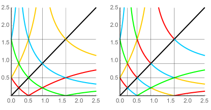
Figure 1: The radial co-motion functions $f_{n}^{\rm SGS}(r)$ from Eq. (49) (left panel, cf. Fig. 6 in Ref. Seidl et al. (2007)) and the equivalent ones, $g_{n}^{\rm SGS}(r)$, Eq. (50) (right panel), for the density of Eq. (47), with $N=5$ electrons in $d=3$ dimensions. Colors: Black, red, yellow, green, blue, respectively, for $n=1,2,3,4,5$.

As an example in $d=3$, consider the density

$$\rho(r)=\frac{N}{4\pi}\frac{e^{-r}}{r^{2}},$$ (47)

for $N$ electrons. In this case, $a_{0}=0$, $a_{N}=\infty$, and

$$N_{\rm e}(r)=N(1-e^{-r}),\qquad R_{\rm e}(\nu)=-\log\Big{(}1-\frac{\nu}{N}\Big{)}.$$ (48)

For $N=5$, Eqs. (45) and (46) yield the functions

$$f_{1}^{\rm SGS}[\rho](r) \equiv\hphantom{\biggl{\{}}r,$$ (49a)

$$f_{2}^{\rm SGS}[\rho](r) =\begin{cases}-\log\big{(}\frac{8}{5}-e^{-r}\big{)}&\big{(}r\leq\log\frac{5}{3}\big{)},\\ -\log\big{(}\frac{2}{5}+e^{-r}\big{)}&\big{(}r\geq\log\frac{5}{3}\big{)},\end{cases}$$ (49b)

$$f_{3}^{\rm SGS}[\rho](r) =\begin{cases}-\log\big{(}e^{-r}-\frac{2}{5}\big{)}&\big{(}r<\log\frac{5}{2}\big{)},\\ -\log\big{(}\frac{2}{5}-e^{-r}\big{)}&\big{(}r>\log\frac{5}{2}\big{)},\end{cases}$$ (49c)

$$f_{4}^{\rm SGS}[\rho](r) =\begin{cases}-\log\big{(}\frac{6}{5}-e^{-r}\big{)}&\big{(}r\leq\log 5\big{)},\\ -\log\big{(}\frac{4}{5}+e^{-r}\big{)}&\big{(}r\geq\log 5\big{)},\end{cases}$$ (49d)

$$f_{5}^{\rm SGS}[\rho](r) =\begin{cases}-\log\big{(}e^{-r}-\frac{4}{5}\big{)}&\big{(}r<\log\frac{5}{4}\big{)},\\ -\log\big{(}\frac{4}{5}-e^{-r}\big{)}&\big{(}r>\log\frac{5}{4}\big{)},\end{cases}$$ (49e)

plotted in the left panel of Fig. 1.

Fixed solely by the radial density profile $\rho(r)$, the $f^{\rm SGS}_{n}[\rho](r)$ can be obtained without knowing the angles (31). Notice that each spherical shell $a_{k-1}\leq r<a_{k}$, $k=1,\dotsc,N$ always contains exactly one electron.

III.4 Group relations

While the $f^{\rm SGS}_{n}(r)$ are continuous, see Fig. 1, we may also consider modified radial co-motion functions $g^{\rm SGS}_{n}(r)$ that explicitly satisfy the group relations of Eq. (5),

$$g^{\rm SGS}_{1}(r) \equiv r,$$

$$g^{\rm SGS}_{2}(r) = g(r),$$

$$g^{\rm SGS}_{3}(r) = g(g(r)),\quad\text{etc.}$$ (50)

The elementary co-motion function $g(r)$ here is defined piecewise on each radial interval $I_{k}=(a_{k-1},a_{k})$, with $k=1,\dotsc,N$: For $k<N$, we generally define

$$g(r)=R_{\rm e}\big{(}2k-N_{\rm e}(r)\big{)},\quad r\in I_{k}\quad(k<N).$$ (51)

For $k=N$, we distinguish even from odd values of $N$,

$$g(r)=\left\{\begin{array}[]{l@{\quad}r}R_{\rm e}\big{(}N-N_{\rm e}(r)\big{)}&(\text{$N$ even})\\ R_{\rm e}\big{(}N_{\rm e}(r)-N+1\big{)}&(\text{$N$ odd})\end{array}\right\},\quad r\in I_{N}.$$ (52)

We see that $g$ maps $I_{k}$ to $I_{k+1}$ ($k<N$) and $I_{N}$ to $I_{1}$.

The $g^{\rm SGS}_{n}(r)$ are equivalent to the $f^{\rm SGS}_{n}(r)$, see Fig. 1, in the sense that for all $r\in[a_{0},a_{N}]$ we have

$$\big{\{}g^{\rm SGS}_{1}(r),\dotsc,g^{\rm SGS}_{N}(r)\big{\}}=\big{\{}f^{\rm SGS}_{1}(r),\dotsc,f^{\rm SGS}_{N}(r)\big{\}}.$$ (53)

III.5 A simple consequence

Due to Eqs. (45) and (46), the function $f_{n}^{\rm SGS}[\rho](r)\equiv f_{n}(r)$ maps the interval $I_{1}=[a_{0},a_{1}]$ onto $I_{n}=[a_{n-1},a_{n}]$, either monotonically or anti-monotonically,

$$r\in[a_{0},a_{1}]:\qquad|f^{\prime}_{n}(r)|=(-1)^{n+1}f^{\prime}_{n}(r)$$ (54)

Consequently, for any function $U(r)$, Eq. (35) implies

$$\int_{a_{0}}^{a_{1}}U\big{(}f_{n}(r)\big{)}\mu_{d}(r)dr = (-1)^{n+1}\int_{f_{n}(a_{0})}^{f_{n}(a_{1})}U(s)\mu_{d}(s)ds$$ (55)

$$= \int_{a_{n-1}}^{a_{n}}U(s)\mu_{d}(s)ds.$$

For $U(r)=V(f_{1}(r),\dotsc,f_{N}(r))$, Eq. (55) yields

$$\int_{a_{n-1}}^{a_{n}}V\big{(}f_{1}(s),\dotsc,f_{N}(s)\big{)}\mu_{d}(s)ds=$$

$$\int_{a_{0}}^{a_{1}}V\big{(}f_{1}(r),\dotsc,f_{N}(r)\big{)}\mu_{d}(r)dr,$$ (56)

where we have used the symmetry (129) of the function $V(r_{1},\dotsc,r_{N})$ and the fact that $\{f_{k}(f_{n}(r))\}_{k=1,\dotsc,N}$ is a permutation of $\{f_{k}(r)\}_{k=1,\dotsc,N}$. Consequently, Eq. (37) can be written as Seidl et al. (2007)

$$V^{\rm SGS}_{ee}[\rho]=\int_{a_{0}}^{a_{1}}dr\,J_{d}(r)\,\rho(r)\,V\big{(}f_{1}(r),\dotsc,f_{N}(r)\big{)}.$$ (57)

IV Counterexample to the SGS solution

Let ${\cal P}_{\rm RAD}$ again be the set of all radially symmetric densities in $d$ dimensions. There is no criterion yet for the subsets ${\cal P}_{\rm SGS}\subset{\cal P}_{\rm SCE}\subset{\cal P}_{\rm RAD}$, where ${\cal P}_{\rm SCE}$ only comprises spherically symmetric densities for which in Eq. (7) the infimum is a minimum (i.e., there is an SCE-type minimizer). If such a minimizer has the SGS co-motion functions, the density belongs to ${\cal P}_{\rm SGS}$.

As a counterexample $\rho\notin{\cal P}_{\rm SGS}$, we consider for $N=3$ electrons in $d=3$ the spherical density

$$\rho_{a,\varepsilon}(r)=\begin{cases}\frac{3}{4\pi a\varepsilon}\frac{1}{r^{2}}&(a\leq r\leq b),\\ 0&(\text{elsewhere}),\end{cases}$$ (58)

with two independent parameters $a,\varepsilon>0$ and

$$b=(1+\varepsilon)a\equiv a+\varepsilon a.$$ (59)

For sufficiently small $\varepsilon>0$, we shall see that $\rho_{a,\varepsilon}\notin{\cal P}_{\rm SGS}$. More precisely, we shall find

$$V_{ee}^{\rm SGS}[\rho_{a,\varepsilon}]=V_{ee}^{\rm SIL}[\rho_{a,\varepsilon}]+\frac{\sqrt{3}}{1080}\frac{\varepsilon^{2}}{a}+O(\varepsilon^{3}).$$ (60)

IV.1 The SGS solution

The density of Eq. (58) describes $N=3$ electrons, distributed within a radial shell with inner radius $a_{0}=a$ and outer radius $a_{3}=b$. In this case, Eq. (43) yields the radial distribution function

$$N_{\rm e}(r)=\begin{cases}0&(r\leq a),\\ \frac{3}{\varepsilon a}(r-a)&(a\leq r\leq b),\\ 3&(r\geq b),\end{cases}$$ (61)

implying the intermediate radii $a_{1}=(1+\frac{1}{3}\varepsilon)a$ and $a_{2}=(1+\frac{2}{3}\varepsilon)a$, and the SGS radial co-motion functions

$$f_{1}^{\rm SGS}(r) \equiv\hphantom{\biggl{\{}}r,$$ (62a)

$$f_{2}^{\rm SGS}(r) =\begin{cases}a_{2}-(r-a)&(a\leq r\leq a_{2}),\\ a+(r-a_{2})&(a_{2}\leq r\leq b),\end{cases}$$ (62b)

$$f_{3}^{\rm SGS}(r) =\begin{cases}a_{2}+(r-a)&(a\leq r\leq a_{1}),\\ b-(r-a_{1})&(a_{1}\leq r\leq b).\end{cases}$$ (62c)

These functions, along with the corresponding equivalent functions $g^{\rm SGS}_{n}(r)$ of Eq. (50), are plotted in Fig. 2.

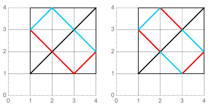
Figure 2: The SGS co-motion functions $f_{n}^{\rm SGS}(r)$ (left panel), Eq. (62), and the equivalent ones $g^{\rm SGS}_{n}(r)$ (right panel) for the density of Eq. (58), with $a=1$ and $\varepsilon=3$. Colors: Black, red, and blue for $n=1,2,3$, respectively. (Cf. Fig. 1.)

IV.1.1 The expectation $\langle\hat{V}_{ee}\rangle$

With these functions in Eq. (57), we obtain

$$\begin{aligned} V_{ee}^{\rm SGS}[\rho_{a,\varepsilon}]&=\int^{\mathrlap{a_{1}}}_{\mathrlap{a}}d{r}\,\frac{3}{\varepsilon a}\,V\Big{(}r,\,a_{2}-r+a,\,a_{2}+r-a\Big{)}\\ &=\frac{3}{a}\int^{\mathrlap{1/3}}_{\mathrlap{0}}d{x}\,V\Big{(}1+\varepsilon x,\\ \end{aligned}\\ 1+\varepsilon\bigl{(}\tfrac{2}{3}-x\bigr{)},1+\varepsilon\bigl{(}\tfrac{2}{3}+x\bigr{)}\Big{)}.$$ (63)

Here we have substituted $r=a(1+\varepsilon x)$ and used the scaling property $V(ar_{1},ar_{2},ar_{3})=\frac{1}{a}V(r_{1},r_{2},r_{3})$. This integral can be evaluated for different values $\varepsilon$ when the minimization of Eq. (30) is performed numerically, cf. Eq. (134). The result is reported in Fig. 3 (blue dots) as a function of $\varepsilon$.

For small $\varepsilon\to 0$, we may use the expansion (141) of the function $V$ in Appendix A (setting $a=1$ there) and integrate analytically in Eq. (63),

$$V_{ee}^{\rm SGS}[\rho_{a,\varepsilon}]=\frac{\sqrt{3}}{a}\Big{[}1-\frac{\varepsilon}{2}+\frac{7}{27}\,\varepsilon^{2}+O(\varepsilon^{3})\Big{]}.$$ (64)

As $\varepsilon\to\infty$, Eq. (63) asymptotically becomes

$$V_{ee}^{\rm SGS}[\rho_{a,\varepsilon}] \to\frac{3}{a}\int^{\mathrlap{1/3}}_{\mathrlap{0}}d{x}\,V\Big{(}\varepsilon x,\varepsilon\bigl{(}\tfrac{2}{3}-x\bigr{)},\varepsilon\bigl{(}\tfrac{2}{3}+x\bigr{)}\Big{)}$$

$$=\frac{3}{a\,\varepsilon}\int^{\mathrlap{1/3}}_{\mathrlap{0}}d{x}\,V\Big{(}x,\tfrac{2}{3}-x,\tfrac{2}{3}+x\Big{)}$$

$$=\frac{3.559}{a\,\varepsilon}.$$ (65)

The expansions (64) and (65) are plotted in Fig. 3 as solid curves.

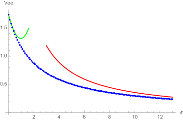
Figure 3: The values $V_{ee}^{\rm SGS}[\rho_{a,\varepsilon}]$ of Eq. (63), plotted for $a=1$ versus $\varepsilon$ (blue dots). Solid curves: The expansions (64) for small $\varepsilon$ (green) and (65) for large $\varepsilon$ (red).

IV.1.2 Hessian matrix of classical potential energy

A necessary (but not sufficient) condition for $\rho\in{\cal P}_{\rm SGS}$, is that the potential energy of Eq. (10) must have a minimum Gori-Giorgi et al. (2009) on the $d$-dimensional set $\Omega^{\rm SGS}_{\rho}$ of Eq. (42). We shall now show that this condition is violated for the density $\rho_{a,\varepsilon}$.

In the case $N=3$, the simplest choice in Eq. (31) is fixing $\theta_{1}=\theta_{2}=\frac{\pi}{2}$ and $\phi_{1}=0$. Then, Eq. (33) implies two numerical functions $\tilde{\phi}_{2}(r)$ and $\tilde{\phi}_{3}(r)$, plus $\tilde{\theta}_{3}(r)\equiv\frac{\pi}{2}$, confining the positions ${\bf f}_{n}^{\rm SGS}[\rho_{a,\varepsilon}](r)$ of Eq. (34) to the $xy$-plane. Eq. (40) for $U(r)=v_{\rm SGS}[\rho](r)$ now yields

$$U^{\prime}(r)=\\ -\sum_{n=2}^{3}\frac{r-f_{n}(r)\cos\tilde{\phi}_{n}(r)}{\bigg{[}\Big{(}r-f_{n}(r)\cos\tilde{\phi}_{n}(r)\Big{)}^{2}+\Big{(}f_{n}(r)\sin\tilde{\phi}_{n}(r)\Big{)}^{2}\bigg{]}^{3/2}}.$$ (66)

This function and its derivative $U^{\prime\prime}(r)$ are readily evaluated numerically.

For simplicity, we treat the problem in 2D, confining the position vectors ${\bf r}_{1},{\bf r}_{2},{\bf r}_{3}$ in Eq. (10) to the $xy$-plane. For the full 3D treatment, see Appendix D.

In terms of the polar coordinates $\{r_{n},\phi_{n}\}_{n=1,\dotsc,N}$ of the $N=3$ electrons in the $xy$-plane, the potential energy function of Eq. (10) for a radial density $\rho(r)$ reads

$$E^{\rm SGS}_{\rm pot}[\rho]({\bf r}_{1},{\bf r}_{2},{\bf r}_{3}) = {\cal C}(\{r_{n},\phi_{n}\})-\sum_{i=1}^{3}U(r_{i})$$ (67)

$$\equiv {\cal E}(\{r_{n},\phi_{n}\}).$$

Here, ${\cal C}$ represents the Coulomb interaction $C_{\rm Coul}$,

$${\cal C}(\{r_{n},\phi_{n}\})\equiv\frac{1}{|{\bf r}_{1}-{\bf r}_{2}|}+\frac{1}{|{\bf r}_{1}-{\bf r}_{3}|}+\frac{1}{|{\bf r}_{2}-{\bf r}_{3}|}=\\ \sum_{i=1}^{2}\sum_{j=i+1}^{3}\Big{[}r_{i}^{2}-2r_{i}r_{j}\cos(\phi_{i}-\phi_{j})+r_{j}^{2}\Big{]}^{-1/2}.$$ (68)

Writing $(r_{1},r_{2},r_{3},\phi_{1},\phi_{2},\phi_{3})=(q_{1},\dotsc,q_{6})\equiv q$, the function ${\cal E}(q)$ should be minimum for $q=q(r)$, where

$$q(r) = \Big{(}r,f_{2}(r),f_{3}(r),0,\tilde{\phi}_{2}(r),\tilde{\phi}_{3}(r)\Big{)}$$ (69)

$$= \Big{(}q_{1}(r),\dotsc,q_{6}(r)\Big{)}.$$

Consequently, in the Taylor expansion

$${\cal E}(q)={\cal E}\big{(}q(r)\big{)}+\\ \frac{1}{2}\sum_{\alpha,\beta=1}^{6}H_{\alpha\beta}(r)\big{(}q_{\alpha}-q_{\alpha}(r)\big{)}\big{(}q_{\beta}-q_{\beta}(r)\big{)}+\dotsb,$$ (70)

the Hessian matrix $H=H(r)$, with the elements

$$H_{\alpha\beta}(r)\equiv\frac{\partial^{2}{\cal E}(q)}{\partial q_{\alpha}\partial q_{\beta}}\Big{|}_{q=q(r)},$$ (71)

should have non-negative eigenvalues only, namely it should have zero eigenvalues in the directions tangential to the manyfold $\Omega^{\rm SGS}_{\rho}$ of Eq. (42), and positive eigenvalues in directions orthogonal to it Gori-Giorgi et al. (2009).

In Ref. Gori-Giorgi et al., 2009 the effect of the electronic kinetic energy in the SIL has been added perturbatively, considering zero-point quantum oscillations around the SCE minimum. Introducing the diagonal matrix

$$M(r)={\rm diag}\big{(}1,1,1,r,f_{2}(r),f_{3}(r)\big{)},$$ (72)

we switch from the coordinates $\delta q=q-q(r)$ to true lengths $u=M\delta q$. Here, $u_{n}$ and $u_{n+3}$, respectively, are the distances on the $xy$-plane travelled by particle $n$ in radial ($r_{n}$-) and in azimuthal ($\phi_{n}$-) direction, when $q$ changes from $q(r)$ to $q(r)+\delta q$. In matrix notation, the quadratic form in Eq. (70) now reads

$$\frac{1}{2}(\delta q)^{T}H(r)(\delta q)=\frac{1}{2}u^{T}K(r)u,$$ (73)

with the new matrix $K(r)=M^{-1}HM^{-1}$. Consequently, the classical equations of motion for the lengths $u$ read

$$m_{e}\ddot{u}=-Ku$$ (74)

(where $m_{e}$ is the electron mass), with the eigenmodes

$$u(t)=e_{\alpha}\sin(\omega_{\alpha}t)\qquad(\alpha=1,\dotsc,6).$$ (75)

Here, $e_{\alpha}$ are the eigenvectors of $K=K(r)$,

$$Ke_{\alpha}=m_{e}\,\omega_{\alpha}^{2}\,e_{\alpha}\qquad(\alpha=1,\dotsc,6).$$ (76)

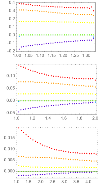
Figure 4: The eigenvalues $m_{e}\,\omega_{\alpha}(r)^{2}$ of the matrix $K=K(r)$ in Eq. (76), plotted versus $r\in[a_{0},a_{1}]$, setting $a\equiv a_{0}=1$, for $\varepsilon=1$ (top), $\varepsilon=3$ (center), and $\varepsilon=10$ (bottom).

The six eigenvalues $m_{e}\,\omega_{\alpha}(r)^{2}$ of $K(r)$ are plotted in Fig. 4 as functions of $r$ for three selected values of $\varepsilon$. We see that for each value of $r$, there are always three positive (red, orange, yellow) and two zero eigenvalues (green and, hidden, blue). In addition, there is always a negative sixth eigenvalue $m_{e}\,\omega_{6}(r)^{2}<0$ (violet), indicating that ${\cal E}(q)$ does not have a minimum on the manyfold $q=q(r)$, revealing that the SGS solution is not optimal for this density. We also notice that the negative eignevalue becomes relatively smaller in magnitude as $\varepsilon$ increases.

Eigenmodes $e_{\alpha}$ with positive eigenvalues $m_{e}\,\omega_{\alpha}^{2}$ describe zero-point oscillations (with angular frequency $\omega_{\alpha}$) of strongly correlated electrons about the strictly correlated limit Seidl (1999); Gori-Giorgi et al. (2009). In 2D, two eigenmodes $e_{\alpha}$ with zero eigenvalues (describing classical motion at constant potential energy) must be expected: either a collective (rigid) 2D rotation of the electrons about the origin ($\alpha=4$) or a collective motion in accordance with the co-motion functions ($\alpha=5$), see Eqs. (41) and (132).

The corresponding 3D analysis (see Appendix D) yields the same six eigenvalues as in 2D (including the negative one), plus two additional zero eigenvalues (since there are two more rotational degrees of freedom in 3D), plus one additional positive eigenvalue.

IV.2 Fractal (FRC) co-motion functions

We now show that, for small $\varepsilon$, a lower expectation of the Coulomb cost (interaction energy) than the SGS one of Eq. (64) can be obtained by using fractal (FRC) co-motion functions. Thus, considering the fractal function $S:[0,1]\to[0,1]$ from Appendix B for the case $N=3$, we construct, for the same density $\rho_{a,\varepsilon}(r)$ of Eq. (58), the radial co-motion functions

$$f^{\rm FRC}_{1}(r) \equiv r,$$ (77a)

$$f^{\rm FRC}_{2}(r) =a+\varepsilon a\cdot S\Bigl{(}\frac{r-a}{\varepsilon a}\Bigr{)},$$ (77b)

$$f^{\rm FRC}_{3}(r) =a+\varepsilon a\cdot S\Bigl{(}S\Bigl{(}\frac{r-a}{\varepsilon a}\Bigr{)}\Bigr{)}.$$ (77c)

Due to Eq. (151), these fractal functions satisfy the group relations of section III.4. Since $x+S(x)+S(S(x))\equiv\frac{3}{2}$, see Eq. (152), they add up to a constant,

$$\sum_{n=1}^{3}f^{\rm FRC}_{n}(r)\;\equiv\;3\frac{a+b}{2}\qquad(a\leq r\leq b).$$ (78)

For the case $a=1$, $b=4$, they are plotted in Fig. 5. Being not differentiable at any point, they cannot satisfy the basic differential equation (35). Nevertheless, they are consistent with the density $\rho_{a,\varepsilon}(r)$, see Appendix C.3.1. Replacing in Eq. (12) the SGS co-motion functions with the FRC ones, we obtain formally

$$\begin{aligned} V_{ee}^{\rm FRC}(a,\varepsilon)&\equiv\widetilde{V}^{\rm SCE}_{ee}\big{[}\rho_{a,\varepsilon},\{{\bf f}^{\rm FRC}_{n}[\rho_{a,\varepsilon}]\}\big{]}\\ &=\int^{\mathrlap{a_{1}}}_{\mathrlap{a}}d{r}\,\frac{3}{\varepsilon a}\,V\Bigl{(}r,\,f^{\rm FRC}_{2}(r),\,f^{\rm FRC}_{3}(r)\Bigr{)}\\ &=\frac{3}{a}\int^{\mathrlap{1/3}}_{\mathrlap{0}}d{x}\,V\Bigl{(}1+\varepsilon x,\end{aligned}\\ 1+\varepsilon S(x),\,1+\varepsilon S\bigl{(}S(x)\bigr{)}\Bigr{)}.$$ (79)

As the function $S(x)$ is highly discontinuous, this integral requires some care. Below, we shall find the expression

$$V_{ee}^{\rm FRC}(a,\varepsilon)=\frac{3}{a}\lim_{k\to\infty}\frac{1}{3^{k}}\sum_{\mathclap{m=1}}^{\mathclap{3^{k-1}}}V\Bigl{(}1+\varepsilon\langle x\rangle_{m},\\ 1+\varepsilon\bigl{\langle}S(x)\bigr{\rangle}_{m},1+\varepsilon\bigl{\langle}S\bigl{(}S(x)\bigr{)}\bigr{\rangle}_{m}\Bigr{)},$$ (80)

using Eq. (86) with $Q(x,y,z)=\frac{3}{a}V(1+\varepsilon x,1+\varepsilon y,1+\varepsilon z)$. Approximating the limit $k\to\infty$ by the finite value $k=5$, we find, for $0<\varepsilon<8.6$, that $V_{ee}^{\rm FRC}(a,\varepsilon)$ is slighlty lower than $V_{ee}^{\rm SGS}[\rho_{a,\varepsilon}]\approx 1.0$, as shown in Fig. 6, where we report the difference $V_{ee}^{\rm FRC}(a,\varepsilon)-V_{ee}^{\rm SGS}[\rho_{a,\varepsilon}]$.

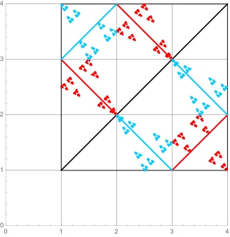
Figure 5: The fractal co-motion functions $f_{n}^{\rm FRC}(r)$, Eq. (77), for the density $\rho_{a,\varepsilon}(r)$ of Eq. (58), with $a=1$ and $\varepsilon=3$. Colors: Black, red (dots) and blue (dots) for $n=1,2,3$, respectively. For comparison, the modified SGS co-motion functions $g_{n}^{\rm SGS}(r)$ from the right panel of Fig. 2 are shown as well.

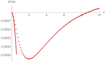
Figure 6: The difference $V_{ee}^{\rm FRC}(a,\varepsilon)-V_{ee}^{\rm SGS}[\rho_{a,\varepsilon}]$ plotted versus $\varepsilon$ (red dots). The corresponding difference between the expansions of Eqs. (64) and (81), Eq. (82), is plotted as a red curve. Notice the small scale on the vertical axis.

In Appendix C.3.1, we find analytically for small $\varepsilon>0$

$$V_{ee}^{\rm FRC}(a,\varepsilon)=\frac{\sqrt{3}}{a}\Bigl{[}1-\frac{\varepsilon}{2}+\frac{31}{120}\varepsilon^{2}+O(\varepsilon^{3})\Bigr{]}.$$ (81)

Subtracting Eq. (64) yields

$$\Delta V_{ee}=V_{ee}^{\rm FRC}-V_{ee}^{\rm SGS}=-\frac{\sqrt{3}}{a}\Bigl{[}\frac{1}{1080}\varepsilon^{2}+O(\varepsilon^{3})\Bigr{]},$$ (82)

proving rigorously that $V_{ee}^{\rm FRC}(a,\varepsilon)<V_{ee}^{\rm SGS}[\rho_{a,\varepsilon}]$ for sufficiently small $\varepsilon>0$ (see the red solid curve in Fig. 6). In particular, a systematic minimization in Appendix C reveals that

$$V_{ee}^{\rm SIL}[\rho_{a,\varepsilon}]=V_{ee}^{\rm FRC}(a,\varepsilon)+O(\varepsilon^{3}).$$ (83)

To derive Eq. (80), we choose an integer $k$, not too small, and divide the interval $[0,1)$ up into the $3^{k}\gg 1$ intervals $I_{m}=[x_{m-1},x_{m})$, with

$$x_{m}=\frac{m}{3^{k}},\qquad m\in\big{\{}0,1,2,\dotsc,3^{k}\big{\}}.$$ (84)

For any function $g(x)$, let $\langle g(x)\rangle_{m}$ be its average value for $x\in I_{m}$. Then, we have

$$x\in I_{m}\Rightarrow\left\{\begin{aligned} \bigl{\lvert}x-\langle x\rangle_{m}\bigr{\rvert}&\leq\frac{1}{2\cdot 3^{k}},\\ \bigl{\lvert}S(x)-\big{\langle}S(x)\big{\rangle}_{m}\bigr{\rvert}&\leq\frac{1}{2\cdot 3^{k}},\\ \bigl{\lvert}S\big{(}S(x)\big{)}-\big{\langle}S\big{(}S(x)\big{)}\big{\rangle}_{m}\bigr{\rvert}&\leq\frac{1}{3^{k}}.\end{aligned}\right.$$ (85)

The second one of these three inequalities is derived in Appendix B. Then, the third one follows immediately from Eq. (152), $x+S(x)+S(S(x))=\frac{3}{2}$.

Consequently, for any continuous function $Q(x,y,z)$, we may define

$$\int^{\mathrlap{1/3}}_{\mathrlap{0}}d{x}\,Q\Bigl{(}x,S(x),S\bigl{(}S(x)\bigr{)}\Bigr{)}$$

$$\equiv\lim_{\mathclap{k\to\infty}}\;\frac{1}{3^{k}}\sum_{\mathclap{m=1}}^{\mathclap{3^{k}/3}}\Big{\langle}Q\Big{(}x,\;S(x),\;S\big{(}S(x)\big{)}\Big{)}\Big{\rangle}_{m}$$

$$=\lim_{\mathclap{k\to\infty}}\;\frac{1}{3^{k}}\sum_{\mathclap{m=1}}^{\mathclap{3^{k}/3}}Q\Bigl{(}\langle x\rangle_{m},\bigl{\langle}S(x)\bigr{\rangle}_{m},\bigl{\langle}S\bigl{(}S(x)\bigr{)}\bigr{\rangle}_{m}\Bigr{)},$$ (86)

where we have applied the mean value theorem in the second step. The average values are given by

$$\langle x\rangle_{m} \equiv \frac{x_{m-1}+x_{m}}{2}=\frac{2m-1}{2\cdot 3^{k}},$$

$$\big{\langle}S(x)\big{\rangle}_{m} = S(x_{m-1}),$$

$$\big{\langle}S\big{(}S(x)\big{)}\big{\rangle}_{m} = \frac{3}{2}-\langle x\rangle_{m}-\big{\langle}S(x)\big{\rangle}_{m}.$$ (87)

The expression for $\langle S(x)\rangle_{m}$ is derived in Appendix B. The one for $\langle S(S(x))\rangle_{m}$ is an immediate consequence of Eq. (152), $x+S(x)+S(S(x))=\frac{3}{2}$.

V Numerical study of the SIL

We investigate here whether the SGS co-motion functions, even when not optimal, provide an approximation that is numerically close to the true SIL. To this end, we first give a short summary of the numerical methods we have used.

V.1 Numerical approaches to SIL

For a numerical approach to the problem of Eq. (27), we assume that $\gamma\in\Pi({\mathbb{R}}^{Nd},\rho)$ can be represented by a regular symmetric function $\gamma({\bf r}_{1},\dotsc,{\bf r}_{N})$. The cost becomes therefore an explicit integration over ${\mathbb{R}}^{Nd}$

$$\langle C\rangle_{\gamma} =\!\int\!d{{\bf r}_{1}}\>\dotsi\!\int\!d{{\bf r}_{N}}\>\gamma({\bf r}_{1},\dotsc,{\bf r}_{N})\,C({\bf r}_{1},\dotsc,{\bf r}_{N})$$

$$=\!\int\!d{{}^{N}{\bf r}}\>\gamma\big{(}\{{\bf r}_{n}\}\big{)}\,C\big{(}\{{\bf r}_{n}\}\big{)},$$ (88)

where ${\bf r}_{n}\in{\mathbb{R}}^{d}$ for $n=1,\dotsc,N$. Similarly, for the constraint we have

$$\pi^{\sharp}_{k}\gamma({\bf r}_{k}) \equiv\!\int\!d{{\bf r}_{1}}\>\dotsi\!\int\!d{{\bf r}_{k-1}}\>\!\int\!d{{\bf r}_{k+1}}\>\dotsi\!\int\!d{{\bf r}_{N}}\>\gamma(\{{\bf r}_{n}\})$$

$$=\frac{\rho({\bf r}_{k})}{N},$$ (89)

Notice that due to the symmetry of the function $\gamma$, it would be sufficient to impose the constraint for only one $k$, as this would imply that the constraint also holds for any $k$. Nevertheless, we keep all constraints explicitly, since it simplifies the forthcoming discussion.

The original minimization problem now becomes

Primal problem: $$V_{ee}^{\rm SIL}[\rho] =\min_{\mathclap{\gamma\in\Pi(\rho)}}\;\langle C\rangle_{\gamma},$$ (90)

where

$$\Pi(\rho)=\bigr{\{}\gamma(\{{\bf r}_{n}\})\in\mathcal{P}({\mathbb{R}}^{dN}):\pi^{\sharp}_{k}\gamma({\bf r})=\rho({\bf r})/N\;\forall_{k}\bigr{\}}.$$ (91)

The constraint that the probability distribution $\gamma$ should yield the density $\rho/N$ as its marginals can be imposed in the following manner

$$V_{ee}^{\rm SIL}[\rho]=\min_{\gamma}\sup_{u}\Biggl{(}\langle C\rangle_{\gamma}+{}\\ \sum_{k=1}^{N}\!\int\!d{{\bf r}}\>u({\bf r})\biggl{(}\frac{\rho({\bf r})}{N}-\pi^{\sharp}_{k}\gamma({\bf r})\biggr{)}\Biggr{)},$$ (92)

where the minimization is now over all symmetric functions. This construction is readily seen to work, since if we had $\pi^{\sharp}_{k}\gamma({\bf r})\neq\rho({\bf r})/N$, then the supremum over $u$ would yield $+\infty$. So only symmetric functions $\gamma$ with the correct density $\rho$ can be candidates for the minimum.

Now if we interchange the minimum and supremum, we get the dual problem

$$V_{ee}^{\text{dual}}[\rho]=\sup_{u}\Biggl{\{}\!\int\!d{{\bf r}}\>u({\bf r})\rho({\bf r})+{}\\ \inf_{\gamma}\!\int\!d{{}^{N}{\bf r}}\>\gamma\big{(}\{{\bf r}_{n}\}\big{)}\Biggl{(}C\big{(}\{{\bf r}_{n}\}\big{)}-\sum_{k=1}^{N}u({\bf r}_{k})\Biggr{)}\Biggr{\}}.$$ (93)

As we now first minimize and only afterwards maximize, we have $V_{ee}^{\text{dual}}[\rho]\leq V_{ee}^{\rm SIL}[\rho]$. Thus, $V_{ee}^{\text{dual}}[\rho]$ provides a lower bound to the primal problem. However, typically one expects that $V_{ee}^{\text{dual}}[\rho]=V_{ee}^{\rm SIL}[\rho]$, which is indeed the case for the Coulomb cost function De Pascale (2015); Buttazzo et al. (2016).

The part between parentheses can now be regarded as a constraint on the maximization of $u$ in the first part. As the probability density $\gamma$ can only be a non-negative function, the infimum only collapses to $-\infty$ if $C<\sum u$. The dual problem can therefore be rewritten as the following constrained maximization

Dual problem: $$V_{ee}^{\text{dual}}[\rho] =\max_{\mathclap{u\in U(C)}}\;\;\!\int\!d{{\bf r}}\>\rho({\bf r})u({\bf r}),$$ (94)

where

$$U(C)=\Bigg{\{}u({\bf r}):\sum_{i=1}^{N}u({\bf r}_{i})\leq C({\bf r}_{1},\dotsc,{\bf r}_{N}),\\ \forall\;({\bf r}_{1},\dotsc,{\bf r}_{N})\in{\mathbb{R}}^{Nd}\Bigg{\}}.$$ (95)

In order to solve numerically (90) and (94), we use a discretization with $M$ equidistant points on the support of marginal as $\{{\bf r}_{j}\}_{j=1,\dotsc,M}$ and define $\rho_{j}=\rho({\bf r}_{j})$. Thus, we get the following discretized problem

$$\min_{\gamma\in\Pi_{k}}\;\;\sum_{\mathclap{j_{1},\dotsc,j_{N}}}c_{j_{1}\dotsc j_{N}}\gamma_{j_{1}\dotsc j_{N}},$$ (96)

where $\Pi_{k}$ is the discretization of $\Pi$ and $c_{j_{1}\dotsc j_{N}}=C({\bf r}_{j_{1}},\dotsc,{\bf r}_{j_{N}})$; the transport plan thus becomes a $M^{N}$ matrix again denoted $\gamma$ with elements $\gamma_{j_{1}\dotsc j_{N}}$. The marginal constraints $\mathcal{C}_{i}$ (such that $\Pi_{k}=\bigcap_{k=1}^{N}\mathcal{C}_{k}$) becomes

$$\mathcal{C}_{k}\equiv\Big{\{}\gamma\in\mathbb{R}_{+}^{M^{N}}:\\ \sum_{\mathclap{j_{1},\dotsc,j_{k-1},j_{k+1},\dotsc,j_{N}}}\gamma_{j_{1}\dotsc j_{N}}=\rho_{j_{k}},\,\forall j_{k}=1,\dotsc,M\Big{\}}.$$ (97)

As a Dirac $\delta$-“function” cannot be represented exactly on a grid, a transport plan $\gamma$ of Monge (or SCE) type (see Sec. II) cannot be truly reproduced. Still, we expect the matrix $\gamma$ to be sparse.

As in the continuous framework we can recover the dual problem given by

$$\begin{split}\max_{u_{j}}&\sum_{j=1}^{M}u_{j}\rho_{j}\\ \text{s.t.}&\sum_{k=1}^{N}u_{j_{k}}\leq c_{j_{1}\dotsc j_{N}}\quad\forall\ j_{k}=1,\dotsc,M,\end{split}$$ (98)

where $u_{j_{k}}=u({\bf r}_{j_{k}})$ is the Kantorovich potential. One can notice that the primal (96) has $M^{N}$ unknowns and $M\times N$ linear constraints and the dual problem (98) has $M$ unknowns, but $M^{N}$ constraints. This actually makes the problems computationally unsolvable with standard linear programming methods even for small cases.

A different approach to the problem (96) consists in adding the entropy of the transport plan $\gamma$. This regularization has been recently introduced in many applications involving optimal transport Cuturi (2013); Benamou et al. (2015, 2016); Galichon and Salanié (2010); Nenna (2016). Thus, we consider the following discrete regularized problem

$$\min_{\gamma\in\mathcal{C}}\;\;\sum_{\mathclap{j_{1},\dotsc,j_{N}}}c_{j_{1}\dotsc j_{N}}\gamma_{j_{1}\dotsc j_{N}}+\text{T}\,\mathcal{E}(\gamma)$$ (99)

where $\mathcal{E}(\gamma)$ is defined as follows

$$\mathcal{E}(\gamma)=\begin{dcases*}\;\;\sum_{\mathclap{j_{1},\dotsc,j_{N}}}\gamma_{j_{1}\dotsc j_{N}}\log(\gamma_{j_{1}\dotsc j_{N}})&if $\gamma\geq 0$\\ +\infty&otherwise,\end{dcases*}$$ (100)

with the convention $0\log 0=0$, $\mathcal{C}$ is the intersection of the set associated to the marginal constraints (we remark that the entropy is a penalization of the non-negative constraint on $\gamma$), and T is a “temperature” (a positive parameter that is kept small). After elementary computations, we can re-write the problem as

$$\min_{\gamma\in\mathcal{C}}\mathcal{H}(\gamma|\bar{\gamma})$$ (101)

where we used the relative entropy

$$\mathcal{H}(\gamma\lvert\bar{\gamma})\equiv\sum_{\mathclap{i_{1},\dotsc,i_{N}}}\gamma_{i_{1}\dotsc i_{N}}\log\left(\frac{\gamma_{i_{1}\dotsc i_{N}}}{\bar{\gamma}_{i_{1}\dotsc i_{N}}}\right)$$ (102)

and $\bar{\gamma}_{i_{1}\dotsc i_{N}}\equiv\exp(-c_{j_{1}\dotsc j_{N}}/\text{T})$.

The entropic regularization spreads the support and this helps to stabilize the computation as it defines a strongly convex program with a unique solution $\gamma_{\text{T}}$. In the limit $\text{T}\to 0$, the regularized solutions $\gamma_{\text{T}}$ converge to $\gamma^{\star}$, the solution of (96) with minimal entropy (see Cominetti and Martín (1994) for a detailed asymptotic analysis and the proof of exponential convergence). It is also interesting, as explained in appendix E, to notice that, in the measure continuous case, the functional (101) can be regarded as a lower bound on the Levy–Lieb functional.

The main advantage of the entropic regularization is that the solution $\gamma_{\text{T}}$ can be obtained through elementary operations and only requires the storage of a few $M$-dimensional vectors. This semi-explicit solution relies on the following proposition (we consider the two marginal case for simplicity).

Proposition V.1.

Problem (101) admits a unique solution $\gamma_{\text{T}}^{\star}$. Moreover, there exists a non-negative vector $a$, uniquely determined up to a multiplicative constant, such that $\gamma_{\text{T}}^{\star}$ has the form

$$(\gamma_{\text{T}}^{\star})_{ij}=a_{i}\bar{\gamma}_{ij}a_{j},$$ (103)

where $\bar{\gamma}_{ij}=\exp(-c_{ij}/\text{T})$. The entries $a_{i}$ are determined by the marginal constraints

$$a_{i}=\dfrac{\rho_{i}}{\sum_{j}\bar{\gamma}_{ij}a_{j}}.$$ (104)

Moreover, the vector can be written as $a_{i}=\exp(u_{i}/\text{T})$ where $u$ is the regularized Kantorovich potential.

It is now clear that one can use Eq. (104) in order to define a fixed point iterative algorithm known as Sinkhorn or Iterative Proportional Fitting Procedure (IPFP)

$$a_{i}^{(n+1)}=\dfrac{\rho_{i}}{\sum_{j}\bar{\gamma}_{ij}a_{j}^{(n)}}.$$ (105)

One can prove the convergence of the Sinkhorn/IPFP algorithm by using the Hilbert metric and the Birkhoff–Bushell theorem. The main idea of this approach lies on the fact that the solution of problem (101) can be seen as the fixed point of a contractive map in the Hilbert metric, see Franklin and Lorentz (1989); Georgiou and Pavon (2015) for a detailed proof. Moreover, one obtains a geometric rate of convergence, and the rate factor can be estimated a priori. The extension to the multi-marginal case is straightforward and we refer the reader to Benamou et al. (2016); Di Marino et al. ; Nenna (2016).

Now we specialize to the spherically symmetric problem with Coulombic cost. As already explained in Sec. III and also Appendix C, the problem can be reduced to one dimensional problem only depending on the radii. The primal problem becomes

Primal problem: $$V_{ee}^{r,\rm SIL}[\mu] =\min_{\mathclap{\beta\in\Pi(\mu)}}\;\langle V\rangle_{\beta},$$ (106)

where the reduced radial cost $V$ is given by Eq. (30) and $\mu(r)=J_{d}(r)\rho(r)$ ($J_{d}$ is the $d$-dimensional Jacobian). Likewise, the dual problem becomes

Dual problem: $$V_{ee}^{r,\text{dual}} =\max_{\mathclap{v\in U(V)}}\;\;\!\int\!d{r}\>\mu(r)v(r).$$ (107)

The discretization of the radial problem proceeds in exactly the same manner as described before.

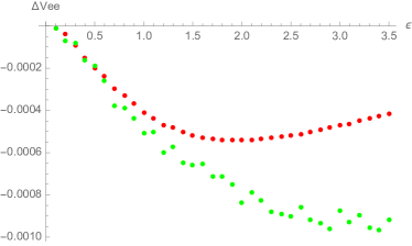
Figure 7: The differences $\widetilde{V}_{ee}^{\rm(method)}(a,\varepsilon)-\widetilde{V}_{ee}^{\rm SGS}(a,\varepsilon)$, plotted versus $\varepsilon$, from the SGS values $\widetilde{V}_{ee}^{\rm SGS}(a,\varepsilon)$ of:
(red) the values $\widetilde{V}_{ee}^{\rm FRC}(a,\varepsilon)$ due to Eq. (80),
(green) the primal values $\widetilde{V}_{ee}^{\rm primal}(a,\varepsilon)$ of  (106).

V.2 Results and comparison with SGS

Consider now the 3-particle density given by (58), for which we want to solve the reduced problem (106). In order to do that, we consider a $M=100$ regular discretization of $[a,b]$, excluding the end-points, thus $r_{i}=a\bigl{(}1+\varepsilon(i-1/2)/M\bigr{)}$. In Fig. 7 we compare the difference between $\tilde{V}_{ee}[\rho_{a,\varepsilon}]$ obtained by solving the primal problem (106) directly and the SGS solution. We see that solving (106) provides an improvement over the SGS maps, but, again, the numerical differences are only in the order of 0.1 %. We have also considered the value of $V_{ee}$ by using the fractal solution (FRC). For thin shells ($\varepsilon\lesssim 0.6$) the primal and FRC perform similarly. For larger shells the primal solution starts to yield a consistently lower value for $V_{ee}$ than the SGS and the fractal solutions. Moreover, around $\varepsilon\approx 1.9$ the supremacy of the FRC solution over the SGS solution starts to deteriorate and its behavior becomes qualitatively different from the primal solution, as expected since it has been shown to be an accurate solution for small $\varepsilon$ only.

As a second example, we consider a $d=3$ sphere of uniform density with $N=3$ electrons. Uniform spheres play an important role in establishing the optimal constant in the Lieb-Oxford inequality Lewin and Lieb (2015); Seidl et al. (2016) and for the low-density uniform electron gas Räsänen et al. (2011); Lewin and Lieb (2015); Seidl et al. (2016). We know that for this density the SGS solution is not optimal, because we still have a small negative eigenvalue in the Hessian (see Sec. IV.1.2). Notice however that SGS has the right density and it is thus a variationally valid “wavefunction”, meaning that the values obtained for the Lieb-Oxford inequality are always rigorous lower bounds for the optimal constant Seidl et al. (2016). The SGS solution has the big advantage of being computationally much cheaper to evaluate than the other methods, making it possible to treat larger particle numbers Seidl et al. (2016); it is thus important to validate its accuracy also when not optimal. We find that $\widetilde{V}_{ee}^{\rm SGS}=2.32682$, while with the entropic regularization method we obtain $\widetilde{V}_{ee}=2.317215$, again a difference of the order of 0.4 %. In Fig. 8 we also show the support of the optimal pair density (i.e., the optimal plan integrated over all variables but two) obtained from the entropic regularization method, compared with the one from SGS. We clearly see that the optimal plan is now different from the SGS one, being much more spread and with a large weight in the top right corner, which corresponds to the case in which the 3 electrons are all almost at the same distance from the center, close to the boundary of the density support.

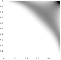
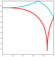
Figure 8: The support of the optimizing pair density from the entropic regularization method (left) and from the SGS ansatz (right) in the case of $N=3$ electrons in a 3-dimensional uniform density within a sphere of radius 1.

An open question is whether there is a way to characterize the class of densities ${\cal P}_{\rm SGS}$ for which the SGS solution is the actual minimizer. To illustrate how puzzling is this question we now solve the problem (106) for the following family of 3-particle densities

$$\rho_{\alpha}({\bf r})=(1-\alpha)\,\rho_{\rm exp}({\bf r})+\alpha\,\rho_{\rm Li}({\bf r}),$$ (108)

where $\rho_{\rm exp}=\frac{3}{\pi}\exp{(-2\,|{\bf r}|)}$, $\rho_{\rm Li}({\bf r})$ is an accurate density for the Lithium atom (exactly the same used by SGS) and $\alpha\in[0,1]$. In Fig. 9, we show the density and the corresponding support of the minimizing pair density: we clearly see a transition from a spread optimal plan to a plan concentrated on the SGS maps, which appear to be the true minimizer in the case of the Li atom density (for which the Hessian eigenvalues were found to be all non-negative in Ref. Gori-Giorgi et al., 2009). In this case we have solved the problem by using both the entropic regularization and the linear programming approach, reporting in Table 1 the corresponding values of the expectation of $V_{ee}$, which confirm the optimality of the SGS solution when $\alpha$ is (close to) 1. Notice, again, that even when not optimal the SGS solution is very close to the LP and entropic values. Also, quite interestingly, when $\alpha$ is close to zero and the plan is spread, it is still concentrated in a region delimited by the SGS solution (see Fig. 1 of Ref. Seidl et al., 2007 and Fig. 1 of this paper). We also checked that for the exponential density a negative eigenvalue in the Hessian of the SGS solution is present for small $r$. The region where the eigenvalue is negative shrinks and diappears as $\alpha\to 1$. It seems that the the shell structure of the Li atom density makes the SGS solution become optimal, but further investigation on this intriguing aspect is needed.

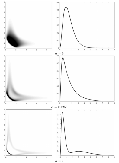
Figure 9: The support of the optimal pair density (left panels) for $N=3$ electrons with radial probability densities $4\pi r^{2}\rho_{\alpha}(r)/N$ (right panels) corresponding to different values of $\alpha$ in Eq. (108). We clearly see that for the Li atom density ($\alpha=1$) the optimal plan is concentrated on the SGS solution, which appears to be optimal in this case (see Fig. 1 in Ref. Seidl et al., 2007).

$\alpha$	LP	$\mathcal{H}$	SGS
0	1.2109	1.2122	1.2178
0.1429	1.2270	1.2284	1.2325
0.2857	1.2471	1.2506	1.2499
0.4286	1.2723	1.2741	1.2723
0.5714	1.3045	1.3064	1.3026
0.7143	1.3462	1.3483	1.3434
0.8571	1.3989	1.4019	1.3902
1	1.4663	1.469	1.4624

Table 1: Values of the expectation of $V_{ee}$ obtained by the Linear Programming approach (LP), the entropic method ($\mathcal{H}$) and the SGS maps for densities of the family (108) with different values of $\alpha$

VI Non-optimal solutions and functional derivative

For radially symmetric densities $\rho(r)$ with $\rho\in{\cal P}_{\rm SGS}$ (see the opening of section IV), the SGS co-motion functions ${\bf f}_{n}^{\rm SGS}[\rho](r)$ provide an optimal solution in Eq. (27), $V^{\rm SIL}_{ee}[\rho]=V^{\rm SGS}_{ee}[\rho]$. The functional $V^{\rm SGS}_{ee}[\rho]$, despite its highly non-local $\rho$-dependence in Eq. (57), has in this case the simple derivative

$$\frac{\delta V^{\rm SGS}_{ee}[\rho]}{\delta\rho(r)}=v_{\rm SGS}[\rho](r),$$ (109)

where the potential $v_{\rm SGS}[\rho](r)$ is readily evaluated from Eq. (40), which provides a powerful shortcut in solving the KS equations with the SCE functional as an approximation for exchange and correlation Mendl et al. (2014).

We shall now prove that Eqs. (109) and (40) are valid for a much more general class of radial densities that include but it is not limited to $\rho\in{\cal P}_{\rm SGS}$, provided that Eq. (114) below is satisfied. For densities $\rho\notin{\cal P}_{\rm SGS}$ the ${\bf f}_{n}^{\rm SGS}[\rho](r)$ do not yield an optimal solution, but, as we have seen from numerical experiments, $V^{\rm SGS}_{ee}[\rho]$ can still serve as a good model for the unknown functional $V^{\rm SIL}_{ee}[\rho]$. Our proof that even in this case the functional derivative is given by Eqs. (109) and (40) uses Eq. (57) for $V^{\rm SGS}_{ee}[\rho]$ and the property (131) of $v_{\rm SGS}[\rho](r)\equiv U(r)$.

Let $\rho_{0}(r)$ be a given radial density, $\rho_{0}\in{\cal P}_{\rm RAD}$, and $\xi(r)$ an arbitrary function with $\int d{\bf r}\,\xi(r)=0$. Considering the series of normalised radial densities

$$\rho_{\varepsilon}(r)=\rho_{0}(r)+\varepsilon\xi(r),$$ (110)

with a small parameter $\varepsilon\in{\mathbb{R}}$, we have to show that

$$\Delta \equiv V^{\rm SGS}_{ee}[\rho_{\varepsilon}]-V^{\rm SGS}_{ee}[\rho_{0}]$$ (111)

$$= \varepsilon\int_{0}^{\infty}dr\,J_{d}(r)\,\xi(r)\,v_{\rm SGS}[\rho_{0}](r)+O(\varepsilon^{2}).$$

Let $f^{\varepsilon}_{1}(r),\dotsc,f^{\varepsilon}_{N}(r)$ be the SGS radial co-motion functions for the density $\rho_{\varepsilon}(r)$. Writing $J_{d}(r)\,\rho_{\varepsilon}(r)=\mu_{\varepsilon}(r)$, Eq. (57) for $V^{\rm SGS}_{ee}[\rho]$ yields

$$\Delta = \int_{a^{\varepsilon}_{0}}^{a^{\varepsilon}_{1}}dr\,\mu_{\varepsilon}(r)\,V\Big{(}f^{\varepsilon}_{1}(r),\dotsc,f^{\varepsilon}_{N}(r)\Big{)}$$ (112)

$$- \int_{a^{0}_{0}}^{a^{0}_{1}}dr\,\mu_{0}(r)\,V\Big{(}f^{0}_{1}(r),\dotsc,f^{0}_{N}(r)\Big{)},$$

where $a^{\varepsilon}_{n}$ are the radii of Eq. (44) for the density $\rho_{\varepsilon}(r)$.

Using the monotonic function $N_{\rm e}^{\varepsilon}(r)=\int_{a^{\varepsilon}_{0}}^{r}ds\,\mu_{\varepsilon}(s)$ and its inverse $R_{\rm e}^{\varepsilon}(\nu)$, we may substitute $N_{\rm e}^{\varepsilon}(r)=\nu$ in the first integral, with $dr\,\mu_{\varepsilon}(r)=d\nu$, and $N_{\rm e}^{0}(r)=\nu$ in the second one, with $dr\,\mu_{0}(r)=d\nu$,

$$\Delta=\int_{0}^{1}d\nu\Big{[}V\Big{(}F^{\varepsilon}_{1}(\nu),\dotsc,F^{\varepsilon}_{N}(\nu)\Big{)}-V\Big{(}F^{0}_{1}(\nu),\dotsc,F^{0}_{N}(\nu)\Big{)}\Big{]},$$ (113)

where $F^{\varepsilon}_{n}(\nu)=f^{\varepsilon}_{n}\big{(}R_{\rm e}^{\varepsilon}(\nu)\big{)}$. When we assume that

$$F^{\varepsilon}_{n}(\nu)-F^{0}_{n}(\nu)=O(\varepsilon)\qquad\mbox{(for all $\nu\in[0,1]$)}$$ (114)

(see the discussion below), we may expand

$$\Delta=\sum_{n=1}^{N}\int_{0}^{1}d\nu\,V_{n}\Big{(}F^{0}_{1}(\nu),\dotsc,F^{0}_{N}(\nu)\Big{)}\big{[}F^{\varepsilon}_{n}(\nu)-F^{0}_{n}(\nu)\big{]}\\ +O(\varepsilon^{2}),$$ (115)

with the notation $V_{n}(r_{1},\dotsc,r_{N})=\frac{\partial}{\partial r_{n}}V(r_{1},\dotsc,r_{N})$. Now Eq. (131), with $v_{\rm SGS}[\rho_{0}](r)\equiv U(r)$, yields

$$\Delta = \sum_{n=1}^{N}\int_{0}^{1}d\nu\,U^{\prime}\big{(}F^{0}_{n}(\nu)\big{)}\big{[}F^{\varepsilon}_{n}(\nu)-F^{0}_{n}(\nu)\big{]}+O(\varepsilon^{2})$$ (116)

$$= \sum_{n=1}^{N}\int_{0}^{1}d\nu\Big{[}U\big{(}F^{\varepsilon}_{n}(\nu)\big{)}-U\big{(}F^{0}_{n}(\nu)\big{)}\Big{]}+O(\varepsilon^{2}),\qquad$$

where, in the second step, we have used Eq. (114) again.

Now, we re-substitute,

$$\Delta=\sum_{n=1}^{N}\Bigg{\{}\int_{a^{\varepsilon}_{0}}^{a^{\varepsilon}_{1}}dr\,\mu_{\varepsilon}(r)\,U\big{(}f^{\varepsilon}_{n}(r)\big{)}\\ -\int_{a^{0}_{0}}^{a^{0}_{1}}dr\,\mu_{0}(r)\,U\big{(}f^{0}_{n}(r)\big{)}\Bigg{\}}+O(\varepsilon^{2}),$$ (117)

and apply Eq. (55) to both integrals,

$$\Delta=\int_{a^{\varepsilon}_{0}}^{a^{\varepsilon}_{N}}dr\,\mu_{\varepsilon}(r)\,U(r)-\int_{a^{0}_{0}}^{a^{0}_{N}}dr\,\mu_{0}(r)\,U(r)+O(\varepsilon^{2}).$$ (118)

Since $\mu_{\varepsilon}(r)=0$ for $r\notin[a^{\varepsilon}_{0},a^{\varepsilon}_{N}]$, we obtain Eq. (111),

$$\Delta=\int_{0}^{\infty}dr\big{[}\mu_{\varepsilon}(r)-\mu_{0}(r)\big{]}\,U(r)+O(\varepsilon^{2}).$$ (119)

Discussion of Eq. (114): Eqs. (46) and (45) for $\nu\in[0,1]$ or, equivalently, for $a_{0}\leq r\leq a_{1}$ yield

$$F^{\varepsilon}_{1}(\nu)=R_{e}^{\varepsilon}(\nu),\hskip 17.07164pt F^{\varepsilon}_{2}(\nu)=R_{e}^{\varepsilon}(2-\nu),$$

$$F^{\varepsilon}_{3}(\nu)=R_{e}^{\varepsilon}(\nu+2), F^{\varepsilon}_{4}(\nu)=R_{e}^{\varepsilon}(4-\nu),$$

$$F^{\varepsilon}_{5}(\nu)=R_{e}^{\varepsilon}(\nu+4), F^{\varepsilon}_{6}(\nu)=R_{e}^{\varepsilon}(6-\nu),$$

$$\ldots\, (0\leq\nu\leq 1).$$ (120)

Therefore, Eq. (114) is true when the expansion

$$R_{\rm e}^{\varepsilon}(\nu)=R_{\rm e}(\nu)+\varepsilon\cdot X(\nu)+O(\varepsilon^{2})\qquad(\nu\in[0,N]),$$ (121)

with $R_{\rm e}(\nu)=R_{\rm e}^{0}(\nu)$, has a finite coefficient $X(\nu)$.

An expression for $X(\nu)$ can be found from

$$\nu\equiv N_{e}^{\varepsilon}\big{(}R_{e}^{\varepsilon}(\nu)\big{)}=\int_{a_{0}^{\varepsilon}}^{R_{e}^{\varepsilon}(\nu)}dr\,\mu_{\varepsilon}(r).$$ (122)

We consider the case when $a_{0}^{\varepsilon}=a_{0}$ is independent of $\varepsilon$. Taking the derivative $\frac{d}{d\varepsilon}$ and then setting $\varepsilon=0$ yields

$$0=\mu_{0}\big{(}R_{e}(\nu)\big{)}\frac{d}{d\varepsilon}R_{e}^{\varepsilon}(\nu)\Big{|}_{\varepsilon=0}+\int_{a_{0}}^{R_{e}(\nu)}dr\,J_{d}(r)\xi(r),$$ (123)

where we have used $\mu_{\varepsilon}(r)=J_{d}(r)[\rho_{0}(r)+\varepsilon\xi(r)]$. Writing $\int_{a_{0}}^{r}ds\,J_{d}(s)\xi(s)\equiv\Xi(r)$, we have

$$X(\nu)\equiv\frac{d}{d\varepsilon}R_{e}^{\varepsilon}(\nu)\Big{|}_{\varepsilon=0}=-\frac{\Xi(R_{e}(\nu))}{\mu_{0}(R_{e}(\nu))}.$$ (124)

Since $\mu_{0}(r)=N^{\prime}_{e}(r)$ and $N_{e}(R_{e}(\nu))\equiv\nu$, we may write

$$X(\nu)=-\Xi\big{(}R_{e}(\nu)\big{)}\,R^{\prime}_{e}(\nu).$$ (125)

Since $R_{e}(\nu)$ and, for any reasonable perturbation $\xi(r)$, also $\Xi(r)$ are bounded functions, $X(\nu)$ is finite for all $\nu\in[0,N]$ when $R^{\prime}_{e}(\nu)$ is. This is a sufficient condition for Eq. (114) to be true.

An example for a case where $R_{e}^{\prime}(\nu)$ is not finite is a density $\rho(r)$ with $\rho(r)=0$ in a finite shell $r_{1}\leq r\leq r_{2}$. Notice again that condition (114) is sufficient but not necessary, and thus its violation does not imply that Eq. (109) cannot hold also in this case.

VII Summary and conclusions

The strictly-correlated (or Monge) solution for the strong-interaction limit provides a physically transparent route to build exchange-correlation functionals with a very non-local density dependence. Its mathematical structure is very different from the usual one of current approximations (which are based on the local density, density gradients, Kohn-Sham local kinetic energy, Hartree-Fock exchange, etc.), and has already inspired new functionals that use some integrals of the density Wagner and Gori-Giorgi (2014); Zhou et al. (2015); Bahmann et al. (2016); Vuckovic et al. (2017).

In this context, an important question, which we have addressed here for the special case of spherically symmetric densities, is whether approximate co-motion functions (or maps) can provide reasonable solutions with a meaningful functional derivative that can be used in the Kohn-Sham equations. In particular, we have shown that

• The co-motion functions conjectured in Ref. Seidl et al., 2007 are not always optimal, but even in the case of non optimality yield an interaction energy that is numerically very close to the minimum one;

• It is very difficult to predict for which spherically symmetric densities the solution of Ref. Seidl et al., 2007 is the actual minimizer (see Fig. 9);

• Even when not optimal, the co-motion functions conjectured in Ref. Seidl et al., 2007 provide a well defined approximation for the Hartree-exchange-correlation energy whose functional derivative can still be computed via the powerful shortcut of Eq. (9).

The fact that a conceptually simple approximation such as SGS Seidl et al. (2007) yields very accurate results for the strong-interaction limit and allows us to compute easily the functional derivative of a highly non-local functional suggests that it might be possible to build new exchange-correlation functionals by using physically motivated approximate co-motion functions, a route that has not been really explored yet. Notice that the results for low density quantum dots of Fig. 1 of Ref. Mendl et al., 2014, which showed very good agreement between the self-consistent KS densities obtained with the SGS functional and the accurate Quantum Monte Carlo values, were obtained for cases in which the SGS co-motion functions are actually not optimal (as shown by a small negative eigenvalue in the Hessian, see Sec. IV.1.2). This is very promising, as it shows that a good approximation for the SIL can be very accurate for systems driven to low density when combined with the KS approach. In future works we will use our results and insight to improve the approximate exchange-correlation functionals proposed in Refs. Wagner and Gori-Giorgi, 2014; Zhou et al., 2015; Bahmann et al., 2016; Vuckovic et al., 2017.

Appendix A The function $V(r_{1},\dotsc,r_{N})$

According to the lines following Eq. (31), the value of the function $V(r_{1},\dotsc,r_{N})$ in Eq. (30) is the minimum electrostatic energy of $N$ equal classical point charges (electrons) that are confined to the surfaces of $N$ concentric spheres with radii $r_{1},\dotsc,r_{N}$, respectively. For its partial derivatives, we here use the notation

$$\frac{\partial V}{\partial r_{i}}=V_{i}(r_{1},\dotsc,r_{N}),\quad\frac{\partial^{2}V}{\partial r_{i}\partial r_{j}}=V_{ij}(r_{1},\dotsc,r_{N}).$$ (126)

A.1 General properties

With the origin ${\bf r}={\bf 0}$ at the center of these spheres, let $\{{\bf r}_{1},\dotsc,{\bf r}_{N}\}$, with $|{\bf r}_{n}|=r_{n}$ for $n=1,\dotsc,N$, be a set of electronic equilibrium positions. (By rigid rotation, an infinite number of equivalent sets can be obtained.) At equilibrium, the force on electron $k$, exerted by the $N-1$ other electrons, must point in radial direction,

$$\sum_{i(\neq k)=1}^{N}\frac{{\bf r}_{k}-{\bf r}_{i}}{|{\bf r}_{k}-{\bf r}_{i}|^{3}}\equiv-\frac{\partial C_{\rm Coul}}{\partial{\bf r}_{k}}=-V_{k}(r_{1},\dotsc,r_{N})\frac{{\bf r}_{k}}{r_{k}}.\qquad$$ (127)

Setting here $k=1$, ${\bf r}_{1}={\bf r}$, and using the SGS positions ${\bf r}_{i}={\bf f}^{\rm SGS}_{i}[\rho](r)$ for a density $\rho\in{\cal P}_{\rm RAD}$, Eq. (38) yields

$$\frac{d}{dr}v_{\rm SGS}[\rho](r)=V_{1}\Big{(}f^{\rm SGS}_{1}[\rho](r),\dotsc,f^{\rm SGS}_{N}[\rho](r)\Big{)}.$$ (128)

Obviously, the function $V$ has the symmetries

$$V(r_{1},\dotsc,r_{N}) = V(r_{\wp(1)},\dotsc,r_{\wp(N)}),$$ (129)

$$V_{k}(r_{1},\dotsc,r_{N}) = V_{\wp(k)}(r_{\wp(1)},\dotsc,r_{\wp(N)}),$$ (130)

where $\wp$ is any permutation of $1,\dotsc,N$. Therefore, writing $v_{\rm SGS}[\rho](r)=U(r)$ and $f^{\rm SGS}_{n}[\rho](r)=f_{n}(r)$, we find

$$U^{\prime}\big{(}f_{i}(r)\big{)}=V_{i}\big{(}f_{1}(r),\dotsc,f_{N}(r)\big{)}\quad(i=1,\dotsc,N).$$ (131)

Consequently, Eq. (41) yields in fact a constant,

$$\frac{d}{dr}\widetilde{E}(r) \equiv \frac{d}{dr}\Big{[}V\big{(}f_{1}(r),\dotsc,f_{N}(r)\big{)}-\sum_{i=1}^{N}U\big{(}f_{i}(r)\big{)}\Big{]}$$ (132)

$$= \sum_{i=1}^{N}\Big{[}V_{i}(f_{1},\dotsc,f_{N})-U^{\prime}(f_{i})\Big{]}f_{i}^{\prime}(r)\;=\;0.\qquad$$

A.2 The case $N=2$

In the case $N=2$, a minimum-energy configuration has the two charges on opposite sides of the origin, with mutual distance $r_{1}+r_{2}$. Therefore, we explicitly have

$$V(r_{1},r_{2})=\frac{1}{r_{1}+r_{2}}.$$ (133)

Eqs. (129), (130) and (127) are readily verified in this case. For Eq. (132), see Eq. (22) in Ref. Seidl (1999).

A.3 The case $N=3$

In the case $N=3$, a minimum-energy configuration has the three charges on a plane containing the origin. For $k=1,2$, let $\theta_{k}$ be the angle between ${\bf r}_{k}$ and ${\bf r}_{3}$. Then,

$$V(r_{1},r_{2},r_{3}) = \min_{\theta_{1},\theta_{2}}\widetilde{V}(r_{1},r_{2},r_{3},\theta_{1},\theta_{2}),$$ (134)

where, due to the cosine theorem,

$$\widetilde{V} \equiv \Big{[}r_{1}^{2}+r_{2}^{2}-2r_{1}r_{2}\cos(\theta_{1}+\theta_{2})\Big{]}^{-1/2}$$ (135)

$$+ \sum_{k=1}^{2}\Big{[}r_{k}^{2}+r_{3}^{2}-2r_{k}r_{3}\cos\theta_{k}\Big{]}^{-1/2}.$$

In the trivial case $r_{3}=0$, we find $\theta_{1}+\theta_{2}=\pi$ and

$$V(r_{1},r_{2},0)=\frac{1}{r_{1}+r_{2}}+\frac{1}{r_{1}}+\frac{1}{r_{2}}.$$ (136)

Finding the general function $V(r_{1},r_{2},r_{3})$ explicitly seems to be a difficult task.

Instead, we shall now evaluate $V$ and its partial derivatives $V_{i}$ and $V_{ij}$ for the case $r_{1},r_{2},r_{3}=a$, when the $N=3$ charges occupy one sphere with radius $a$ and at equilibrium make an equilateral triangle with side length $a\sqrt{3}$,

$$V(a,a,a)=\frac{\sqrt{3}}{a}.$$ (137)

The symmetry of this problem implies for $i=1,2,3$

$$V_{i}(a,a,a) = \frac{1}{3}\sum_{k=1}^{3}V_{k}(a,a,a)$$ (138)

$$= \frac{1}{3}\frac{d}{da}V(a,a,a)=-\frac{1}{\sqrt{3}}\,a^{-2},$$

and, since $V_{12}(a,a,a)=V_{23}(a,a,a)=V_{13}(a,a,a)$, as well as $V_{11}(a,a,a)=V_{22}(a,a,a)=V_{33}(a,a,a)$,

$$\frac{2}{\sqrt{3}}\,a^{-3} \equiv \frac{d}{da}V_{i}(a,a,a)$$ (139)

$$= \sum_{k=1}^{3}V_{ik}(a,a,a)$$

$$= V_{33}(a,a,a)+2V_{12}(a,a,a).$$

Since $V_{33}(a,a,a)=\frac{4}{5\sqrt{3}}\,a^{-3}$, Eq. (148) below, we have

$$V_{12}(a,a,a)=\frac{3}{5\sqrt{3}}\,a^{-3}.$$ (140)

In summary, we obtain the Taylor expansion

$$V(r_{1},r_{2},r_{3}) = \frac{\sqrt{3}}{a}\Big{[}1-\frac{u_{1}+u_{2}+u_{3}}{3a}$$ (141)

$$+ \frac{u_{1}u_{2}+u_{1}u_{3}+u_{2}u_{3}}{5a^{2}}+2\frac{u_{1}^{2}+u_{2}^{2}+u_{3}^{2}}{15a^{2}}$$

$$+ O\Big{(}\frac{u_{1}}{a},\frac{u_{2}}{a},\frac{u_{3}}{a}\Big{)}^{3}\Big{]},$$

where $u_{i}=r_{i}-a$.

To find $V_{33}(a,a,a)=\frac{d^{2}}{dr^{2}}V(a,a,r)|_{r=a}$, we observe that any equilibrium configuration with $r_{1}=r_{2}=a$ has equal angles $\theta_{1}=\theta_{2}\equiv\theta$. In this case, Eq. (135) reads

$$\widetilde{V}=\frac{1}{a}\Big{\{}\frac{1}{2\sin\theta}+\frac{2}{\sqrt{1+s^{2}-2s\cos\theta}}\Big{\}}\equiv\frac{\widetilde{W}(s,\theta)}{a},$$ (142)

with the new variable $s=\frac{r_{3}}{a}$. For $s=1$, the equilibrium angle is $\theta=\frac{2\pi}{3}$. For $\widetilde{W}(s,\frac{2\pi}{3}+\alpha)\equiv W(s,\alpha)$, the addition theorems yield

$$W(s,\alpha) = \frac{1}{\sqrt{3}\cos\alpha-\sin\alpha}$$ (143)

$$+2\Big{[}1+s^{2}+s\big{(}\cos\alpha+\sqrt{3}\sin\alpha\big{)}\Big{]}^{-1/2}$$

$$= W(s,0)+\sum_{n=1}^{\infty}W_{n}(s)\alpha^{n}.$$

The equilibrium angle $\alpha(s)$ is fixed by $\frac{\partial}{\partial\alpha}W(s,\alpha)=0$,

$$0=W_{1}(s)+2W_{2}(s)\alpha(s)+3W_{3}(s)\alpha(s)^{2}+\dotsb$$ (144)

Taking the derivative $\frac{d}{ds}$ yields

$$0 = W^{\prime}_{1}(s)+2\Big{[}W^{\prime}_{2}(s)\alpha(s)+W_{2}(s)\alpha^{\prime}(s)\Big{]}$$ (145)

$$+ 3\Big{[}W^{\prime}_{3}(s)\alpha(s)+2W_{3}(s)\alpha^{\prime}(s)\Big{]}\alpha(s)+\dotsb$$

Setting $s=1$ and using $\alpha(1)=0$, we obtain

$$\alpha^{\prime}(1)=-\frac{W^{\prime}_{1}(1)}{2W_{2}(1)}=-\frac{\sqrt{3}}{15},$$ (146)

where we have used $W_{1}(s)=\frac{1}{3}-s\sqrt{3}(1+s+s^{2})^{-3/2}$ and $W_{2}(s)=\frac{5}{6\sqrt{3}}+\frac{1}{4}(2s+11s^{2}+2s^{3})(1+s+s^{2})^{-5/2}$. Eventually, we find

$$V_{33}(a,a,a) \equiv \frac{d^{2}}{dr^{2}}V(a,a,r)\Big{|}_{r=a}$$ (147)

$$= \frac{1}{a^{2}}\frac{d^{2}}{ds^{2}}\,\frac{W\big{(}s,\alpha(s)\big{)}}{a}\Big{|}_{s=1}$$

$$= \frac{1}{a^{3}}\Big{[}\frac{\partial^{2}W}{\partial s^{2}}+2\frac{\partial^{2}W}{\partial s\partial\alpha}\alpha^{\prime}(s)+$$

$$\frac{\partial^{2}W}{\partial\alpha^{2}}\alpha^{\prime}(s)^{2}+\frac{\partial W}{\partial\alpha}\alpha^{\prime\prime}(s)\Big{]}\Big{|}_{s=1}.\qquad$$

The partial derivatives of $W=W(s,\alpha)$ are readily evaluated from Eq. (143). As expected, $\frac{\partial W}{\partial\alpha}|_{s=1}=0$. With Eq. (146), the remaining three terms in Eq. (147) yield

$$V_{33}(a,a,a)=\frac{4}{5\sqrt{3}}a^{-3}.$$ (148)

Appendix B The functions $S(x)$

For a given $N=2,3,4,\dotsc$, each real number $x\in[0,1]$ always has a unique representation in the form

$$x=\sum_{\ell=1}^{\infty}\frac{n_{\ell}}{N^{\ell}},\qquad n_{\ell}\in\{0,1,2,\dotsc,N-1\}.$$ (149)

$n_{\ell}$ is the $\ell$-th digit of the $N$-fraction representing $x$ (decimal fraction when $N=10$). We define $S(x)$ as the function that raises each digit of $x$ by 1. More precisely, in terms of the particular permutation $\wp$ with $\wp(n_{\ell})=n_{\ell}+1$ for $0\leq n_{\ell}\leq N-2$ and $\wp(N-1)=0$, we define

$$S(x)\equiv S\bigg{(}\sum_{\ell=1}^{\infty}\frac{n_{\ell}}{N^{\ell}}\bigg{)}=\sum_{\ell=1}^{\infty}\frac{\wp(n_{\ell})}{N^{\ell}}.$$ (150)

Since $\wp^{N}(n_{\ell})=n_{\ell}$, we then trivially have

$$S^{N}(x)\equiv\sum_{\ell=1}^{\infty}\frac{\wp^{N}(n_{\ell})}{N^{\ell}}=x.$$ (151)

Since $\{\wp(n_{\ell}),\wp^{2}(n_{\ell}),\dotsc,\wp^{N}(n_{\ell})\}=\{0,1,\dotsc,N-1\}$, we similarly obtain

$$\sum_{n=1}^{N}S^{n}(x) = \sum_{n=1}^{N}\left(\sum_{\ell=1}^{\infty}\frac{\wp^{n}(n_{\ell})}{N^{\ell}}\right)$$ (152)

$$= \sum_{\ell=1}^{\infty}\frac{1}{N^{\ell}}\left(\sum_{n=0}^{N-1}n\right)=\frac{N}{2}.$$

In the case $N=2$, Eq. (152) implies

$$S(x)=1-x.$$ (153)

In the cases $N\geq 3$, in contrast, $S(x)$ is a discontinuous function whose graph is a fractal.

To see this, we consider for $x\in[0,1]$ and $k=1,2,3,\dotsc$ the functions $T_{k}(x)$, that raise only the $k$-th digit of $x$ by 1 and leave all other digits unchanged. Formally,

$$T_{k}(x)=\sum_{\ell=1}^{k-1}\frac{n_{\ell}}{N^{\ell}}+\frac{\wp(n_{k})}{N^{k}}+\sum_{\ell=k+1}^{\infty}\frac{n_{\ell}}{N^{\ell}}.$$ (154)

An explicit expression, valid for $x<1$, is easily found: For $y\in{\mathbb{R}}$, let $[y]$ be the largest integer with $[y]\leq y$ and consider the function $U:{\mathbb{R}}\to{\mathbb{R}}$, $y\mapsto U(y)$, with

$$U(y)=\left\{\begin{array}[]{ccc}y+\frac{1}{N}&&\big{(}y-[y]<\frac{N-1}{N}\big{)},\\ &&\\ y-\frac{N-1}{N}&&\big{(}y-[y]\geq\frac{N-1}{N}\big{)}.\end{array}\right.$$ (155)

Then, for $0\leq x<1$, we have

$$T_{k}(x)=\frac{U(N^{k-1}x)}{N^{k-1}}\qquad(0\leq x<1).$$ (156)

$T_{1}(x)$, $T_{2}(x)$ and $T_{3}(x)$ are plotted in Fig. 10 for the cases $N=2$ and $N=3$. Obviously,

$$\lim_{k\to\infty}T_{k}(x)\equiv x.$$ (157)

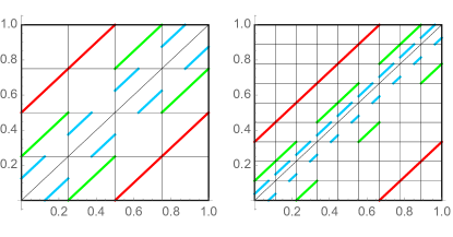
Figure 10: The functions $T_{1}(x)$, $T_{2}(x)$, and $T_{3}(x)$ (in red, green, and blue, respectively) for the cases $N=2$ (left panel) and $N=3$ (right panel).

By composition, we define further functions,

$$S_{k}(x)=T_{k}(T_{k-1}(\dotso\,T_{1}(x)\dotso))\qquad(k=1,2,3,\dotsc).$$ (158)

$S_{1}(x)$, $S_{2}(x)$ and $S_{3}(x)$ are plotted in Fig. 11 for the cases $N=2$ and $N=3$. By definition,

$$\lim_{k\to\infty}S_{k}(x)=S(x).$$ (159)

Fig. 11 clearly illustrates for $N=2$ that $S_{k}(x)\to 1-x$ as $k\to\infty$, while for $N=3$ the graph of $S_{k}(x)$ becomes a fractal in that limit.

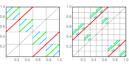
Figure 11: The functions $S_{1}(x)\equiv T_{1}(x)$, $S_{2}(x)$, and $S_{3}(x)$ (in red, green, and blue, respectively) for the cases $N=2$ (left panel) and $N=3$ (right panel).

Focusing on the case $N=3$, we now derive Eqs. (85) and (87). In terms of the equidistant numbers

$$x_{m}=\frac{m}{3^{k}},\qquad m\in\big{\{}0,1,2,\dotsc,3^{k}\big{\}},$$ (160)

we consider the intervals $I_{m}=[x_{m-1},x_{m})$.

Any $x\in I_{m}$ has a unique representation

$$x=\underbrace{\sum_{\ell=1}^{k}\frac{n_{\ell}}{3^{\ell}}}_{\displaystyle x_{m-1}}+\sum_{\ell=k+1}^{\infty}\frac{n_{\ell}(x)}{3^{\ell}},$$ (161)

where, for a fixed value of $m$, the first $k$ coefficients $n_{1},\dotsc,n_{k}$ do not depend on $x$. By definition, we have

$$S(x) = \sum_{\ell=1}^{k}\frac{\wp(n_{\ell})}{3^{\ell}}+\sum_{\ell=k+1}^{\infty}\frac{\wp(n_{\ell}(x))}{3^{\ell}}$$ (162)

$$= S(x_{m-1})+\sum_{\ell=k+1}^{\infty}\frac{\wp(n_{\ell}(x))-1}{3^{\ell}}.$$

In the second step, we have used $\wp(0)=1$, implying that

$$S(x_{m-1})=\sum_{\ell=1}^{k}\frac{\wp(n_{\ell})}{3^{\ell}}+\sum_{\ell=k+1}^{\infty}\frac{1}{3^{\ell}}.$$ (163)

The permutation $\wp$ in the case $N=3$ is given by

$$\wp(0)=1,\quad\wp(1)=2,\quad\wp(2)=0.$$ (164)

Averaging Eq. (162) over all $x\in I_{m}$ yields Eq. (87),

$$\big{\langle}S(x)\big{\rangle}_{m}=S(x_{m-1}),$$ (165)

since for each $\ell\geq k+1$, $\wp(n_{\ell}(x))$ assumes its values 0, 1 or 2 with equal probabilites, $\langle\wp(n_{\ell}(x))-1\rangle_{m}=0$. Moreover, for $x\in I_{m}$, we find Eq. (85),

$$\Big{|}S(x)-\big{\langle}S(x)\big{\rangle}_{m}\Big{|}\leq\sum_{\ell=k+1}^{\infty}\frac{1}{3^{\ell}}=\frac{1}{2\cdot 3^{k}}.$$ (166)

Appendix C Systematic minimization in Eq. (27)

C.1 Simplification for spherical densities $\rho(r)$

For convenience, we focus here on the case with $d=3$ dimensions. When $\rho$ is a spherical density, $\rho\in{\cal P}_{\rm RAD}$, any probability measure $\gamma\in\Pi({\mathbb{R}}^{3N},\rho)$, formally written as a regular function $\gamma({\bf r}_{1},\dotsc,{\bf r}_{N})$ here, corresponds to a simpler one $\beta\in\Pi({\mathbb{P}}^{N},\mu)$, given by

$$\beta(r_{1},\dotsc,r_{N})=r_{1}^{2}\dotsm r_{N}^{2}\int d\Omega_{1}\dotsi\int d\Omega_{N}\,\gamma({\bf r}_{1},\dotsc,{\bf r}_{N}).$$ (167)

Here, ${\mathbb{P}}={\mathbb{R}}_{0}^{+}$ and $\mu(r)=4\pi r^{2}\rho(r)$. $\beta$ has the $N$ identical marginals $\frac{\mu(r)}{N}$. In particular, we have

$$\langle V\rangle_{\gamma} = \int^{\mathrlap{\infty}}_{\mathrlap{0}}d{r_{1}}\,\dotsi\int^{\mathrlap{\infty}}_{\mathrlap{0}}d{r_{N}}\,\beta(r_{1},\dotsc,r_{N})\,V(r_{1},\dotsc,r_{N})$$ (168)

$$\equiv \langle V\rangle_{\beta},$$

and Eq. (27) can be written as Seidl et al. (2007)

$$V^{\rm SIL}_{ee}[\rho]\;=\;\min_{\beta\in\Pi({\mathbb{P}}^{N},\mu)}\big{\langle}V\big{\rangle}_{\beta}.$$ (169)

Example: The Monge (or SCE) type measure $\gamma=\gamma^{\rm SGS}$ describing the SGS ansatz of section III corresponds to

$$\beta^{\rm SGS}(r_{1},\dotsc,r_{N})=\frac{\mu(r_{1})}{N}\prod_{n=2}^{N}\delta\big{(}r_{n}-f^{\rm SGS}_{n}(r_{1})\big{)}.$$ (170)

Despite not looking symmetric at first glance, $\beta^{\rm SGS}$ does have the correct $N$ identical marginals: (i) Obviously, $\!\int\!d{r_{2}}\>\dotsi\!\int\!d{r_{N}}\>\,\beta^{\rm SGS}(r_{1},\dotsc,r_{N})=\frac{\mu(r_{1})}{N}$, and (ii) we also have, e.g.,

$$\!\int\!d{r_{1}}\>\!\int\!d{r_{3}}\>\dotsi\!\int\!d{r_{N}}\>\beta^{\rm SGS}(r_{1},\dotsc,r_{N})\\ =\!\int\!d{r_{1}}\>\frac{\mu(r_{1})}{N}\,\delta\big{(}r_{2}-f_{2}(r_{1})\big{)}=\frac{\frac{\mu(r_{0})}{N}}{\lvert f^{\prime}_{2}(r_{0})\rvert},\qquad$$ (171)

where, due to a well known rule for the $\delta$-function, $r_{0}$ is the radius satisfying $r_{2}-f_{2}(r_{0})=0$. Employing Eq. (35), we therefore correctly find

$$\frac{\frac{\mu(r_{0})}{N}}{\lvert f^{\prime}_{2}(r_{0})\rvert}=\frac{\mu\big{(}f_{2}(r_{0})\big{)}}{N}=\frac{\mu(r_{2})}{N}.$$ (172)

C.2 Application to the density $\rho_{a,\varepsilon}(r)$ of Eq. (58)

We shall now perform the minimization in Eq. (169) for the density $\rho=\rho_{a,\varepsilon}$ of Eq. (58), when $N=3$ and $\mu(r)=\mu_{a,\varepsilon}(r)\equiv 4\pi r^{2}\rho_{a,\varepsilon}(r)=\frac{N}{a\varepsilon}$ for $a\leq r\leq a(1+\varepsilon)$. Any $\beta\in\Pi({\mathbb{P}}^{3},\mu_{a,\varepsilon})$ has the identical marginals

$$\frac{\mu_{a,\varepsilon}(r_{k})}{3}\equiv\int^{\mathrlap{b}}_{\mathrlap{a}}d{r_{i}}\,\int^{\mathrlap{b}}_{\mathrlap{a}}d{r_{j}}\,\beta(r_{1},r_{2},r_{3})=\frac{1}{a\varepsilon},$$ (173)

where $b=a(1+\varepsilon)$ and $\{i,j,k\}=\{1,2,3\}$.

Substituting in Eq. (168) $r_{n}=a+\varepsilon ax_{n}$, $x_{n}\in[0,1]$, and rearranging quadratic terms in the Taylor expansion of $V(r_{1},r_{2},r_{3})$, Eq. (141), we obtain

$$\langle V\rangle_{\beta}=\int^{\mathrlap{1}}_{\mathrlap{0}}d{x_{1}}\,\int^{\mathrlap{1}}_{\mathrlap{0}}d{x_{2}}\,\int^{\mathrlap{1}}_{\mathrlap{0}}d{x_{3}}\,(\varepsilon a)^{3}\tilde{\beta}(x_{1},x_{2},x_{3})\times{}$$

$$\left[\sum_{k=1}^{3}v_{\rm sep}^{(\varepsilon)}(x_{k})+\frac{\sqrt{3}\varepsilon^{2}}{10a}(x_{1}+x_{2}+x_{3})^{2}+V_{\rm res}^{(\varepsilon)}\right],\quad$$ (174)

with $v_{\rm sep}^{(\varepsilon)}(x)=\frac{\sqrt{3}}{3a}(1-\varepsilon x+\frac{\varepsilon^{2}}{10}x^{2})$ and a residual term

$$V_{\rm res}^{(\varepsilon)}(x_{1},x_{2},x_{3})=O(\varepsilon^{3}).$$ (175)

For $\tilde{\beta}(\{x_{n}\})=\beta(\{a+\varepsilon ax_{n}\})$, Eq. (173) implies

$$\int^{\mathrlap{1}}_{\mathrlap{0}}d{x_{i}}\,\int^{\mathrlap{1}}_{\mathrlap{0}}d{x_{j}}\,\tilde{\beta}(x_{1},x_{2},x_{3})=\frac{1}{(\varepsilon a)^{3}}\qquad(i\neq j),$$ (176)

and the first term in Eq. (174) can be integrated, yielding

$$\sum_{k=1}^{3}\int^{\mathrlap{1}}_{\mathrlap{0}}d{x_{k}}\,v_{\rm sep}^{(\varepsilon)}(x_{k})=\frac{\sqrt{3}}{a}\Big{[}1-\frac{\varepsilon}{2}+\frac{\varepsilon^{2}}{30}\Big{]},$$ (177)

cf. Eq. (28) for separable interactions. Since this result does not depend on $\beta$, Eq. (169) now reads

$$V_{ee}^{\rm SIL}[\rho_{a,\varepsilon}]=\frac{\sqrt{3}}{a}\Big{[}1-\frac{\varepsilon}{2}+\frac{\varepsilon^{2}}{30}\Big{]}+\\ +\min_{\beta\in\Pi({\mathbb{P}}^{3},\mu_{a,\varepsilon})}\Big{\langle}\frac{\sqrt{3}\varepsilon^{2}}{10a}C_{h}+V_{\rm res}^{(\varepsilon)}\Big{\rangle}_{\beta},$$ (178)

where, in terms of the convex function $h(x)=x^{2}$,

$$C_{h}(x_{1},x_{2},x_{3}) \equiv (x_{1}+x_{2}+x_{3})^{2}$$ (179)

$$= h(x_{1}+x_{2}+x_{3}).$$

Any series of minimizers $\beta_{\varepsilon}$ in Eq. (178) converges for $\varepsilon\to 0$ to a minimizer of $\langle C_{h}\rangle$, since $V_{\rm res}^{(\varepsilon)}=O(\varepsilon^{3})$,

$$V_{ee}^{\rm SIL}[\rho_{a,\varepsilon}]=\frac{\sqrt{3}}{a}\Big{[}1-\frac{\varepsilon}{2}+\frac{\varepsilon^{2}}{30}\Big{]}+\\ +\frac{\sqrt{3}\varepsilon^{2}}{10a}\min_{\beta\in\Pi({\mathbb{P}}^{3},\mu_{a,\varepsilon})}\big{\langle}C_{h}\big{\rangle}_{\beta}+O(\varepsilon^{3}).$$ (180)

In the next section we study the minimization problem for $\big{\langle}C_{h}\big{\rangle}$, showing necessary and sufficient conditions that a minimizer should satisfy, which are violated by the SGS ansatz (for details and a complete proof see Gerolin (2016)). In particular this will imply that SGS solutions are also not minimizers for $V_{ee}^{\rm SIL}[\rho_{a,\varepsilon}]$ if $\varepsilon$ is small enough.

Moreover, we also show three different examples of minimizers for the repulsive harmonic cost in the one-dimensional case that can be used as trial plans for $V_{ee}^{\rm SIL}[\rho_{a,\varepsilon}]$ for small $\varepsilon$.

A similar proof of the fact that SGS minimizers are not always minimizers in (1)) was also obtained by Colombo and Stra Colombo and Stra (2016), who also showed that $\rho\in{\cal P}_{\rm SGS}\neq\emptyset$.

C.3 Cost $h(x_{1}+x_{2}+x_{3})$ with $h$ convex

Now, we consider cost functions $C_{h}(x_{1},x_{2},x_{3})=h(x_{1}+x_{2}+x_{3})$, $h$ convex. We will show that for this class of cost functions, we can construct examples of $SCE$-type minimizers and non $SCE$-type minimizers.

To find a minimizer of $\langle C_{h}\rangle_{\beta}$, we consider a particular $\beta=\beta_{0}\in\Pi({\mathbb{P}}^{3},\mu_{a,\varepsilon})$ which is concentrated on the hyperplane $H=\{(x_{1},x_{2},x_{3})\,|\,x_{1}+x_{2}+x_{3}=NX\}$, thus fixing the average value $X$ of the $N=3$ coordinates $x_{1},x_{2},x_{3}$. In this case, we obviously have

$$\int(x_{1}+x_{2}+x_{3})\,d\beta_{0}=NX,\qquad\langle C_{h}\rangle_{\beta_{0}}=h(NX).$$ (181)

For a general $\beta\in\Pi({\mathbb{P}}^{3},\mu_{a,\varepsilon})$, Eq. (28) implies

$$\int(x_{1}+x_{2}+x_{3})\,d\beta=\sum_{k=1}^{N}\int_{a}^{b}dr_{k}\,\frac{\mu_{a,\varepsilon}(r_{k})}{N}\,x_{k}\equiv N\bar{x}.$$ (182)

Consequently, the fixed average value $X$, dictated by $\beta_{0}$, must satisfy $X=\bar{x}\equiv\frac{\bar{r}-a}{\varepsilon a}=\frac{1}{2}$, with the barycenter $\bar{r}$ of the density $\mu_{a,\varepsilon}(r)$,

$$\bar{r}\equiv\int_{a}^{b}dr\,\frac{\mu_{a,\varepsilon}(r)}{N}\,r=\frac{1}{\varepsilon a}\frac{b^{2}-a^{2}}{2}=\frac{a+b}{2}.$$ (183)

Moreover, Jensen’s inequality for convex functions yields

$$\langle C_{h}\rangle_{\beta} \equiv \int h(x_{1}+x_{2}+x_{3})\,d\beta$$ (184)

$$\geq h\left(\int(x_{1}+x_{2}+x_{3})\,d\beta\right)$$

$$= h(N\bar{x})\equiv h(NX)=\langle C_{h}\rangle_{\beta_{0}}.$$

In other words, $\beta_{0}$ is a minimizer,

$$\min_{\beta\in\Pi({\mathbb{P}}^{3},\mu_{a,\varepsilon})}\langle C_{h}\rangle_{\beta}=h(N\bar{x})=\Big{(}3\cdot\frac{1}{2}\Big{)}^{2}=\frac{9}{4},$$ (185)

and Eq. (180) yields

$$V_{ee}^{\rm SIL}[\rho_{a,\varepsilon}]=\frac{\sqrt{3}}{a}\Big{[}1-\frac{\varepsilon}{2}+\frac{31}{120}\varepsilon^{2}+O(\varepsilon^{3})\Big{]}.$$ (186)

We shall now construct different examples for measures $\beta_{0}\in\Pi({\mathbb{P}}^{3},\mu_{a,\varepsilon})$ that are concentrated on the hyperplane $H$ and, therefore, are minimizers of $\langle C_{h}\rangle_{\beta}$ in Eq. (180). For all these examples, we conclude

$$\langle V\rangle_{\beta_{0}}=V_{ee}^{\rm SIL}[\rho_{a,\varepsilon}]+O(\varepsilon^{3}).$$ (187)

C.3.1 An SCE-type minimizer

We now use the fractal co-motion functions $f^{\rm FRC}_{n}(r)$ of Eq. (77) to construct an SCE-type probability measure $\beta^{\rm FRC}$ with the identical marginals $\frac{\mu_{a,\varepsilon}(r)}{N}\equiv\frac{1}{\varepsilon a}$, implying that $\beta^{\rm FRC}\in\Pi({\mathbb{P}}^{3},\mu_{a,\varepsilon})$. In other words, despite being fractal, the co-motion functions $f^{\rm FRC}_{n}(r)$ do belong to an SCE state with the smooth density $\rho_{a,\varepsilon}(r)$ of Eq. (58).

In a second step, we shall see further below, that $\beta^{\rm FRC}$ is a minimizer of $\langle C_{h}\rangle_{\beta}$ in Eq. (180).

The fractal function $S(x)$ in Eq. (77) is the (uniform) limit $k\to\infty$ of the piecewise linear functions $S_{k}(x)$ in Eq. (158). Replacing in Eq. (77) $S(x)$ with $S_{k}(x)$, for some finite $k\in{\mathbb{N}}$, we obtain piecewise linear functions

$$f^{\rm FRC}_{k,1}(r) \equiv r,$$ (188a)

$$f^{\rm FRC}_{k,2}(r) =a+\varepsilon a\cdot S_{k}\Bigl{(}\frac{r-a}{\varepsilon a}\Bigr{)},$$ (188b)

$$f^{\rm FRC}_{k,3}(r) =a+\varepsilon a\cdot S_{k}\Bigl{(}S_{k}\Bigl{(}\frac{r-a}{\varepsilon a}\Bigr{)}\Bigr{)},$$ (188c)

for $r\in[a,b]$, with piecewise constant derivatives

$$\frac{d}{dr}f^{\rm FRC}_{k,n}(r)=1,\qquad r\in(c_{m-1},c_{m}),$$ (189)

where $c_{m}=a+m\frac{b-a}{3^{k}}$ and $m=1,\dotsc,3^{k}$. For $k=2$, these three functions are plotted in Fig. 12 (upper panel).

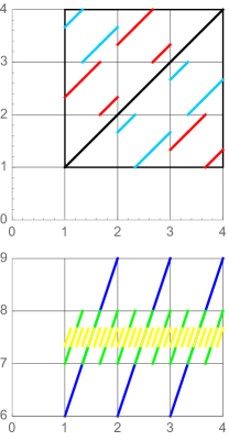
Figure 12: Upper panel: The functions $f^{\rm FRC}_{k,1}(r)=r$, $f^{\rm FRC}_{k,2}(r)$, and $f^{\rm FRC}_{k,3}(r)=f^{\rm FRC}_{k,2}(f^{\rm FRC}_{k,2}(r))$ for $k=2$ (in black, red and blue, respectively) in the case $a=1$, $\varepsilon=3$ when $r\in[1,4]$.
Lower panel: The functions $\psi^{\rm FRC}_{k}(r)=\sum_{n=1}^{3}f^{\rm FRC}_{k,n}(r)$, for $k=1$ (dark-blue), $k=2$ (green) and $k=3$ (yellow), indicating that the limiting function is a constant, $\psi^{\rm FRC}_{\infty}(r)=\frac{15}{2}$.

For a given $k\geq 2$, consider for any radial interval $I=[r_{A},r_{B}]\subseteq[a,b]$ the “strictly correlated” subset

$$\Omega(I)=\left\{\Big{(}r,f^{\rm FRC}_{k,2}(r),f^{\rm FRC}_{k,3}(r)\Big{)}\,\Big{|}\,r\in I\right\}\subseteq{\mathbb{P}}^{3}$$ (190)

of the radial configuration space ${\mathbb{P}}^{3}=\{(r_{1},r_{2},r_{3})\}$. A particular probability measure $\beta_{k}^{\rm FRC}$ on ${\mathbb{P}}^{3}$ is specified when we assign to the subsets $\Omega(I)$ the probabilities

$$p_{\Omega(I)}\equiv\int_{\Omega(I)}d\beta_{k}^{\rm FRC}=\frac{r_{B}-r_{A}}{b-a},$$ (191)

since then $p_{\Omega([a,b])}=1$, and any subset $\Omega\subset{\mathbb{P}}^{3}$ with $\Omega\cap\Omega([a,b])=\emptyset$ has zero probability. This means that the probability measure $\beta_{k}^{\rm FRC}$ is of the SCE-type.

Now, it is easy to see that $\beta^{\rm FRC}_{k}\in\Pi({\mathbb{P}}^{3},\mu_{a,\varepsilon})$: In the configurations $(r_{1},r_{2},r_{3})\in\Omega(I)$, each one of the two coordinates $r_{2}$ and $r_{3}$ covers a finite set of no more than $3^{k}$ disjoint subintervals of $[a,b]$. Due to Eq. (189), the lengths of these disjoint intervals in both cases add up to the length $r_{B}-r_{A}$ of $I$. Therefore, $r_{1}$, $r_{2}$, and $r_{3}$ all have the same uniform radial probability density

$$\frac{p_{\Omega(I)}}{r_{B}-r_{A}}=\frac{1}{b-a}=\frac{1}{\varepsilon a}\equiv\frac{\mu_{a,\varepsilon}(r)}{N}.$$ (192)

Furthermore, any SCE-type $\beta\in\Pi({\mathbb{P}}^{3},\mu_{a,\varepsilon})$ is concentrated on the hyperplane $H$ with $r_{1}+r_{2}+r_{3}=3\bar{r}\equiv 3\frac{a+b}{2}$, and therefore is a minimizer in Eq. (185), when its radial co-motion functions $f_{n}(r)$ add up to a constant.

$$\sum_{n=1}^{3}f_{n}(r)=3\bar{r}\equiv 3\frac{a+b}{2}\qquad(a\leq r\leq b).$$ (193)

This condition is violated by the SGS co-motion functions $f^{\rm SGS}_{n}(r)$ for the density $\rho_{a,\varepsilon}$, see Eq. (62), but also by the present ones $f^{\rm FRC}_{k,n}(r)$, see the lower panel of Fig. 12. In the limit $k\to\infty$, however, when the fractal functions $f^{\rm FRC}_{n}(r)$ of Eq. (77) are recovered, the condition is satisfied, see Eq. (78).

C.3.2 Non-SCE type minimizers

We now consider (Example 4.13 in Di Marino et al. ) a probability measure $\beta_{0}$ with the (almost continuous) co-motion functions $f^{\rm VIO}_{1}(r)\equiv r$ and

$$f_{2}^{\rm VIO}(r) = \left\{\begin{array}[]{cc}r+\bar{r}-a&\quad(a\leq r<\bar{r})\\ r+a-\bar{r}&\quad(\bar{r}\leq r\leq b)\end{array}\right\},$$ (196)

$$f_{3}^{\rm VIO}(r) = \left\{\begin{array}[]{cc}2a+b-2r&\quad(a\leq r<\bar{r})\\ a+2b-2r&\quad(\bar{r}\leq r\leq b)\end{array}\right\}.$$ (199)

Since they satisfy Eq. (193), this $\beta_{0}$ is concentrated on $H$ and therefore a minimizer. However, the functions $f_{n}^{\rm VIO}(r)$ violate the group relations of section III.4. They do not describe a true SCE state, since $f_{3}^{\rm VIO}(r)$ is not an injective function, relating each radius $r_{3}=f_{3}^{\rm VIO}(r_{1})$ to two different values of $r_{1}$. Consistently, these functions do not satisfy the SCE basic differential equation (35).

Another minimizer $\beta_{0}\in\Pi({\mathbb{P}}^{N},\mu)$ (concentrated on $H$) which is not of the SCE type at all, is given by

$$\beta_{0}(r_{1},r_{2},r_{3})=\frac{4}{(\varepsilon a)^{3}}\delta(r_{1}+r_{2}+r_{3}-3\bar{r})\times$$

$$\times\max\Big{(}|r_{1}-\bar{r}|,|r_{2}-\bar{r}|,|r_{3}-\bar{r}|\Big{)}.$$ (200)

The $\delta$-function guarantees that $\beta_{0}$ is concentrated on $H$ and therefore is certainly a minimizer in Eq. (180). However, it is not of the SCE type, since each one of the radii $r_{2}$ and $r_{3}$ can, at fixed radius $r_{1}$, assume arbitrary values. Only their sum $r_{2}+r_{3}$ is fixed by $r_{1}$.

To show that $\beta_{0}$ has the correct uniform marginals $\frac{\mu(r_{k})}{N}=\frac{1}{\varepsilon a}$, it is convenient to switch from $r_{n}\in[a,b]$ to shifted coordinates $s_{n}=r_{n}-\bar{r}\in[-c,c]$, where $c=\frac{1}{2}\varepsilon a$,

$$\tilde{\beta}_{0}(s_{1},s_{2},s_{3})=\frac{4}{(\varepsilon a)^{3}}\delta(s_{1}+s_{2}+s_{3})\max\Big{(}|s_{1}|,|s_{2}|,|s_{3}|\Big{)}.$$ (201)

Obviously, it is sufficient to consider

$$\frac{\mu(r_{1})}{N} = \int_{-c}^{c}ds_{2}\int_{-c}^{c}ds_{3}\,\tilde{\beta}_{0}(s_{1},s_{2},s_{3})$$ (202)

$$= \frac{4}{(\varepsilon a)^{3}}\int_{-c}^{c}ds_{2}\,\theta\Big{(}c-|s_{1}+s_{2}|\Big{)}\times$$

$$\times\max\Big{(}|s_{1}|,|s_{2}|,|s_{1}+s_{2}|\Big{)}.$$

Here, $\theta$ is the Heavyside step function, with $\theta(s)=1$ for $s\geq 0$ and $\theta(s)=0$ otherwise. We first consider the case $s_{1}\geq 0$, when $\theta(c-|s_{1}+s_{2}|)=0$ for $s_{2}>c-s_{1}$,

$$\frac{\mu(r_{1})}{N} = \frac{4}{(\varepsilon a)^{3}}\int_{-c}^{c-s_{1}}ds_{2}\,\max\Big{(}|s_{1}|,|s_{2}|,|s_{1}+s_{2}|\Big{)}$$ (203)

$$= \frac{4}{(\varepsilon a)^{3}}\int_{-c}^{-s_{1}}ds_{2}|s_{2}|$$

$$+ \frac{4}{(\varepsilon a)^{3}}\int_{-s_{1}}^{0}ds_{2}|s_{1}|$$

$$+ \frac{4}{(\varepsilon a)^{3}}\int_{0}^{c-s_{1}}ds_{2}|s_{1}+s_{2}|\qquad(s_{1}\geq 0).$$

In the latter three integrals, we may write, respectively, $|s_{2}|=-s_{2}$, $|s_{1}|=s_{1}$, $|s_{1}+s_{2}|=s_{1}+s_{2}$, to find

$$\frac{\mu(r_{1})}{N}=\frac{1}{\varepsilon a}.$$ (204)

A similar analysis yields the same result for $s_{1}\leq 0$.

Appendix D Hessian matrix in 3D

For the 3D treatment of the problem in section IV.1.2, we use spherical polar coordinates $\{r_{n},\theta_{n},\phi_{n}\}_{n=1,2,3}$ for the vectors ${\bf r}_{n}$ in Eq. (10). Then, Eq. (67) becomes

$$E^{\rm SGS}_{\rm pot}[\rho]({\bf r}_{1},{\bf r}_{2},{\bf r}_{3}) = {\cal C}(\{r_{n},\theta_{n},\phi_{n}\})-\sum_{i=1}^{3}U(r_{i})$$ (205)

$$\equiv {\cal E}(\{r_{n},\theta_{n},\phi_{n}\}),$$

where, instead of Eq. (68), we now have

$${\cal C}(\{r_{n},\theta_{n},\phi_{n}\})=\sum_{i=1}^{2}\sum_{j=i+1}^{3}\Big{[}r_{i}^{2}-2r_{i}r_{j}\cos\gamma_{ij}+r_{j}^{2}\Big{]}^{-1/2},$$ (206)

with the angle $\gamma_{ij}$ between the vectors ${\bf r}_{i}$ and ${\bf r}_{j}$,

$$\cos\gamma_{ij}=\sin\theta_{i}\sin\theta_{j}\cos(\phi_{i}-\phi_{j})+\cos\theta_{i}\cos\theta_{j}.$$ (207)

Writing $(r_{1},r_{2},r_{3},\phi_{1},\phi_{2},\phi_{3},\theta_{1},\theta_{2},\theta_{3})=(q_{1},\dotsc,q_{9})\equiv q$, the function ${\cal E}(q)$ should be minimum for $q=q(r)$,

$$q(r) = \Big{(}r,f_{2}(r),f_{3}(r),0,\tilde{\phi}_{2}(r),\tilde{\phi}_{3}(r),{\textstyle\frac{\pi}{2},\frac{\pi}{2},\frac{\pi}{2}}\Big{)}$$ (208)

$$= \Big{(}q_{1}(r),\dotsc,q_{9}(r)\Big{)}.$$

The corresponding Hessian matrix $H^{9\times 9}(r)$, given by

$$H_{\alpha\beta}^{9\times 9}(r)=\frac{\partial^{2}{\cal E}(q)}{\partial q_{\alpha}\partial q_{\beta}}\Big{|}_{q=q(r)}\qquad(\alpha,\beta=1,\dotsc,9),$$ (209)

has block form: When $q_{\alpha}\in\{r_{1},r_{2},r_{3},\phi_{1},\phi_{2},\phi_{3}\}$ and $q_{\beta}\in\{\theta_{1},\theta_{2},\theta_{3}\}$, we easily verify from Eq. (206) that

$$H_{\alpha\beta}^{9\times 9}(r)\equiv\frac{\partial^{2}{\cal C}(q)}{\partial q_{\alpha}\partial q_{\beta}}\Big{|}_{q=q(r)}=0.$$ (210)

On the other hand, we obviously have

$$H_{\alpha\beta}^{9\times 9}(r)=H_{\alpha\beta}(r)\qquad(\alpha,\beta\leq 6),$$ (211)

with the corresponding $(6\times 6)$-matrix $H(r)$ from the 2D treatment of section IV.1.2. Consequently, six eigenvalues of $H^{9\times 9}(r)$ are identical with the ones of $H(r)$, and the remaining three eigenvalues are identical with the ones of the $(3\times 3)$-matrix $H^{(\theta)}(r)$, given by

$$H_{ij}^{(\theta)}(r)=\frac{\partial^{2}{\cal C}(q)}{\partial\theta_{i}\partial\theta_{j}}\Big{|}_{q=q(r)}\qquad(i,j=1,2,3).$$ (212)

The frequencies $\omega_{\alpha}$ of the new eigenmodes $e_{7,8,9}$ are obtained from the eigenvalues $m\,\omega_{\alpha}^{2}$ of the $(3\times 3)$-matrix $K^{(\theta)}(r)=M^{-1}H^{(\theta)}M^{-1}$, with the diagonal matrix $M={\rm diag}(r,f_{2}(r),f_{3}(r))$.

Appendix E An entropic inequality

Consider the $N-$marginals Monge-Kantorovich (namely $V_{ee}^{\rm SIL}$) problem with the Coulomb cost and all marginals equal to $\rho({\bf r})$ (where we have assumed that $\rho$ is a measure absolutely continuous with respect the $d-$dimensional Lebesgue measure)

$$V_{ee}^{\rm SIL}[\rho]=\min_{\gamma\in\Pi({\mathbb{R}}^{Nd},\rho)}\langle C_{\rm Coul}\rangle_{\gamma},$$ (213)

and the entropic regularization

$$\mathscr{S}_{N,\text{T}}[\rho]\equiv\min_{\gamma\in\Pi({\mathbb{R}}^{Nd},\rho)}\mathcal{H}(\gamma|\eta_{\text{T}}),$$ (214)

where $\eta_{\text{T}}\equiv\frac{1}{L}\exp{(-\sum_{i<j}\frac{1}{\text{T}|{\bf r}_{i}-{\bf r}_{j}|})}\otimes_{i=1}^{K}d{\bf r}_{i}$ ($L$ is the normalization constant) and the relative entropy is defined as

$$\mathcal{H}(\mu|\nu)=\!\int\!d{{\bf r}}\>\mu\log(\frac{\mu}{\nu}).$$

We show now that problem (214) with a fixed parameter T is a lower bound of the Levy-Lieb functional.
Take a plan $\gamma({\bf r}_{1},\cdots,{\bf r}_{N})=|\psi({\bf r}_{1},\cdots,{\bf r}_{N})|^{2}$ (it is obvious that $\sqrt{\gamma}\in\text{H}^{1}({\mathbb{R}}^{Nd})$), then the Levy-Lieb functional $F^{LL}[\rho]$ reads as

$$F^{LL}[\rho]\equiv\inf_{\gamma\in\Pi({\mathbb{R}}^{Nd},\rho)}\dfrac{\hbar^{2}}{2}\!\int\!d{{\bf r}_{1}}\>\dotsi\!\int\!d{{\bf r}_{N}}\>|\nabla\sqrt{\gamma}|^{2}+\langle C_{\rm Coul}\rangle_{\gamma}.$$ (215)

We can establish the following result

Theorem E.1 (Entropy Lower bound,Di Marino and Nenna ; Nenna (2016)).

Let be $\rho\in\mathcal{P}({\mathbb{R}}^{d})$ and $\psi\in\text{H}^{1}({\mathbb{R}}^{Nd};{\mathbb{R}})$, then the following inequality holds

$$F^{LL}[\rho]\geq\mathscr{S}_{N,\text{T}}[\rho],$$ (216)

with $\text{T}=\dfrac{\pi\hbar^{2}}{2}$.

In order to prove theorem E.1 we need some useful results on the logarithmic Sobolev inequality (LSI) for the Lebesgue measure.

Corollary E.2 (Corollary 7.3, Gozlan and Léonard (2010)).

Let us consider $\nu\in\mathcal{P}(\mathbb{R}^{d})$ such that $\nu({\bf r})=e^{-V({\bf r})}$ with $\operatorname{D}^{2}V\geq\kappa Id$. Then, for every $f\geq 0$ such that $f\nu\in\mathcal{P}(\mathbb{R}^{d})$ we have that

$$\mathcal{H}(f\nu|\nu)\leq\frac{2}{\kappa}\int|\nabla\sqrt{f}|^{2}\,d\nu.$$ (217)

Notice that, thanks to the $1$-homogeneity of both sides of the inequality with respect to $f$, one can forget the constraint $f\nu\in\mathcal{P}({\mathbb{R}}^{d})$. Now we are ready to state our result for the Lebesgue measure:

Theorem E.3 (LSI,Di Marino and Nenna ; Nenna (2016)).

Let $f\geq 0$ be a function such that $\sqrt{f}\in\text{H}^{1}(\mathbb{R}^{d})$ and $f\mathcal{L}^{d}\in\mathcal{P}({\mathbb{R}}^{d})$. Then the following holds:

$$\mathcal{H}(f\mathcal{L}^{d}|\mathcal{L}^{d})\leq\frac{1}{\pi}\!\int\!d{{\bf r}_{1}}\>|\nabla\sqrt{f}|^{2}.$$ (218)

Proof.

The proof is rather simple: it relies on the observation that if $\int f\,d\nu\leq 1$ then $\mathcal{H}(f\nu|\nu)\geq\int f\log f\,d\nu$. In particular we can consider the measure $\nu_{{\bf r}_{2}}=e^{-\pi|{\bf r}_{1}-{\bf r}_{2}|^{2}}$. Since (218) is again $1$-homogeneous in both sides, we can suppose that $\!\int\!d{{\bf r}_{1}}\>f=1$. It is clear that, since $\nu_{{\bf r}_{2}}\leq\mathcal{L}^{d}$, we have that $\int f\,d\nu_{{\bf r}_{2}}\leq 1$ for every ${\bf r}_{2}$. In particular, we have that

$$\!\int\!d{\nu_{{\bf r}_{2}}}\>f\log f\ \leq\mathcal{H}(f\nu_{{\bf r}_{2}}|\nu_{{\bf r}_{2}}).$$

Now we can integrate this with respect to ${\bf r}_{2}$ and use that $\!\int\!d{{\bf r}_{2}}\>e^{-\pi|{\bf r}_{1}-{\bf r}_{2}|^{2}}=1$ to obtain

$$\!\int\!d{{\bf r}_{1}}\>f\log f\leq\!\int\!d{{\bf r}_{2}}\>\mathcal{H}(f\nu_{{\bf r}_{2}}|\nu_{{\bf r}_{2}}).$$

Now considering $V({\bf r}_{1})=\pi|{\bf r}_{1}-{\bf r}_{2}|^{2}$, we have $\operatorname{D}^{2}V=2\pi Id$ and in particular we have that (217) holds with $\kappa=2\pi$ and so we conclude

$$\begin{split}&\mathcal{H}(f\mathcal{L}^{d}|\mathcal{L}^{d})=\!\int\!d{{\bf r}_{1}}\>f\log f\leq\\ &\dfrac{1}{\pi}\int\int\,d\nu_{{\bf r}_{2}}\,d{\bf r}_{2}|\nabla\sqrt{f}|^{2}=\\ &\dfrac{1}{\pi}\!\int\!d{{\bf r}_{1}}\>|\nabla\sqrt{f}|^{2}.\end{split}$$ (219)

∎

Proof Theorem E.1.

Notice that by definition $\gamma\geq 0$ and $\gamma\in\text{H}^{1}({\mathbb{R}}^{Nd})$ so we can apply theorem E.3 and we have

$$\dfrac{\hbar^{2}}{2}\!\int\!d{{\bf r}_{1}}\>\dotsi\!\int\!d{{\bf r}_{N}}\>|\nabla_{{\bf r}}\sqrt{\gamma}|^{2}\geq\text{T}\mathcal{H}(\gamma|\mathcal{L}^{dN}),$$ (220)

where $\text{T}\equiv\dfrac{\pi\hbar^{2}}{2}$. It follows that

$$\begin{split}&\!\int\!d{{\bf r}_{1}}\>\dotsi\!\int\!d{{\bf r}_{N}}\>|\nabla_{{\bf r}}\sqrt{\gamma({\bf r}_{1}\cdots{\bf r}_{N})}|^{2}+\\ &\!\int\!d{{\bf r}_{1}}\>\dotsi\!\int\!d{{\bf r}_{N}}\>\sum_{i<j}\dfrac{1}{|{\bf r}_{i}-{\bf r}_{j}|}\gamma({\bf r}_{1}\cdots{\bf r}_{N})\geq\\ &\text{T}\mathcal{H}(\gamma|\mathcal{L}^{dN})+\!\int\!d{{\bf r}_{1}}\>\dotsi\!\int\!d{{\bf r}_{N}}\>\sum_{i<j}\dfrac{1}{|{\bf r}_{i}-{\bf r}_{j}|}\gamma({\bf r}_{1}\cdots{\bf r}_{N})=\\ &\mathcal{H}(\gamma|\eta_{\text{T}}),\end{split}$$ (221)

where $\eta_{\text{T}}=\exp{(-\sum_{i<j}\frac{1}{\text{T}|{\bf r}_{i}-{\bf r}_{j}|})}\otimes_{i=1}^{N}d{{\bf r}_{i}}$ (notice that w.l.o.g. we can normalize $\eta_{\text{T}}$ in order to have a probability measure). Then, the inequality (216) easily follows. ∎

References

- Seidl (1999) M. Seidl, Phys. Rev. A 60, 4387 (1999).
- Seidl et al. (1999) M. Seidl, J. P. Perdew, and M. Levy, Phys. Rev. A 59, 51 (1999).
- Seidl et al. (2007) M. Seidl, P. Gori-Giorgi, and A. Savin, Phys. Rev. A 75, 042511 (2007).
- Gori-Giorgi et al. (2009) P. Gori-Giorgi, G. Vignale, and M. Seidl, J. Chem. Theory Comput. 5, 743 (2009).
- Levy (1979) M. Levy, Proc. Natl. Acad. Sci. U.S.A. 76, 6062 (1979).
- Cotar et al. (2013) C. Cotar, G. Friesecke, and C. Klüppelberg, Comm. Pure Appl. Math. 66, 548 (2013).
- Colombo and Di Marino (2013) M. Colombo and S. Di Marino, in Annali di Matematica Pura ad Applicata (Springer, Berlin Heidelberg, 2013) pp. 1–14.
- Malet and Gori-Giorgi (2012) F. Malet and P. Gori-Giorgi, Phys. Rev. Lett. 109, 246402 (2012).
- Malet et al. (2013) F. Malet, A. Mirtschink, J. C. Cremon, S. M. Reimann, and P. Gori-Giorgi, Phys. Rev. B 87, 115146 (2013).
- Mendl et al. (2014) C. B. Mendl, F. Malet, and P. Gori-Giorgi, Phys. Rev. B 89, 125106 (2014).
- Colombo et al. (2015) M. Colombo, L. De Pascale, and S. Di Marino, Can. J. Math. 67, 350 (2015).
- Buttazzo et al. (2012) G. Buttazzo, L. De Pascale, and P. Gori-Giorgi, Phys. Rev. A 85, 062502 (2012).
- Mirtschink et al. (2012) A. Mirtschink, M. Seidl, and P. Gori-Giorgi, J. Chem. Theory Comput. 8, 3097 (2012).
- Vuckovic et al. (2016) S. Vuckovic, T. J. P. Irons, A. Savin, A. M. Teale, and P. Gori-Giorgi, J. Chem. Theory Comput. 12, 2598 (2016).
- Malet et al. (2015) F. Malet, A. Mirtschink, C. B. Mendl, J. Bjerlin, E. O. Karabulut, S. M. Reimann, and P. Gori-Giorgi, Phys. Rev. Lett. 115, 033006 (2015).
- Colombo and Stra (2016) M. Colombo and F. Stra, Math. Models Methods Appl. Sci. 26, 1025 (2016).
- Note (1) is a compact set. Consequently, since is a linear (thus continuous) functional of , Eq. (17\@@italiccorr) is truly a minimum, not only an infimum.
- Monge (1781) G. Monge, Mémoire sur la théorie des déblais et des remblais (Histoire Acad. Sciences, Paris, 1781).
- Brenier (1991) Y. Brenier, Communications on pure and applied mathematics 44, 375 (1991).
- Caffarelli et al. (2002) L. Caffarelli, M. Feldman, and R. McCann, J. Amer. Math. Soc , 1 (2002).
- Trudinger and Wang (2001) N. Trudinger and X.-J. Wang, Calc. Var. Paritial Differential Equations , 19 (2001).
- Kantorovich (1942) L. V. Kantorovich, Dokl. Akad. Nauk. SSSR. 37, 227 (1942).
- De Pascale (2015) L. De Pascale, ESAIM: Mathematical Modelling and Numerical Analysis 49, 1643 (2015).
- Buttazzo et al. (2016) G. Buttazzo, T. Champion, and L. De Pascale, arXiv preprint arXiv:1608.08780 (2016).
- Cuturi (2013) M. Cuturi, in Advances in Neural Information Processing Systems (2013) pp. 2292–2300.
- Benamou et al. (2015) J.-D. Benamou, G. Carlier, M. Cuturi, L. Nenna, and G. Peyré, SIAM Journal on Scientific Computing 37, A1111 (2015).
- Benamou et al. (2016) J.-D. Benamou, G. Carlier, and L. Nenna, “A numerical method to solve multi-marginal optimal transport problems with coulomb cost,” in Splitting Methods in Communication, Imaging, Science, and Engineering, edited by R. Glowinski, S. J. Osher, and W. Yin (Springer International Publishing, Cham, 2016) pp. 577–601.
- Galichon and Salanié (2010) A. Galichon and B. Salanié, CEPR Discussion Paper (2010).
- Nenna (2016) L. Nenna, Numerical Methods for Multi-Marginal Opimal Transportation, Ph.D. thesis, Université Paris-Dauphine (2016).
- Cominetti and Martín (1994) R. Cominetti and J. S. Martín, Mathematical Programming 67, 169 (1994).
- Franklin and Lorentz (1989) J. Franklin and J. Lorentz, Linear Algebra and its Applications 114–115, 717 (1989).
- Georgiou and Pavon (2015) T. T. Georgiou and M. Pavon, Journal of Mathematical Physics 56, 033301 (2015).
- (33) S. Di Marino, A. Gerolin, and L. Nenna, pre-print arXiv:1506.04565 .
- Lewin and Lieb (2015) M. Lewin and E. H. Lieb, Phys. Rev. A 91, 022507 (2015).
- Seidl et al. (2016) M. Seidl, S. Vuckovic, and P. Gori-Giorgi, Mol. Phys. 114, 1076 (2016).
- Räsänen et al. (2011) E. Räsänen, M. Seidl, and P. Gori-Giorgi, Phys. Rev. B 83, 195111 (2011).
- Wagner and Gori-Giorgi (2014) L. O. Wagner and P. Gori-Giorgi, Phys. Rev. A 90, 052512 (2014).
- Zhou et al. (2015) Y. Zhou, H. Bahmann, and M. Ernzerhof, J. Chem. Phys. 143, 124103 (2015).
- Bahmann et al. (2016) H. Bahmann, Y. Zhou, and M. Ernzerhof, J. Chem. Phys. 145, 124104 (2016).
- Vuckovic et al. (2017) S. Vuckovic, T. J. P. Irons, L. O. Wagner, A. M. Teale, and P. Gori-Giorgi, Phys. Chem. Chem. Phys. (2017).
- Gerolin (2016) A. Gerolin, Multimarginal optimal transport and potential optimization problems for Schrödinger operators, Ph.D. thesis, Università degli studi di Pisa (2016).
- (42) S. Di Marino and L. Nenna, in preparation .
- Gozlan and Léonard (2010) N. Gozlan and C. Léonard, Markov Processes and Related Fields 16, 635 (2010).