Cross-Mode Interference Characterization in Cellular Networks with Voronoi Guard Regions

Abstract

Advances in cellular networks such as device-to-device communications and full-duplex radios, as well as the inherent elimination of intra-cell interference achieved by network-controlled multiple access schemes, motivates the investigation of the cross-mode interference properties under a guard region corresponding to the Voronoi cell of an access point (AP). By modeling the positions of interfering APs and user equipments (UEs) as Poisson distributed, analytical expressions for the statistics of the cross-mode interference generated by either APs or UEs are obtained based on appropriately defined density functions. The considered system model and analysis are general enough to capture many operational scenarios of practical interest, including conventional downlink/uplink transmissions with nearest AP association, as well as transmissions where not both communicating nodes lie within the same cell. Analysis provides insights on the level of protection offered by a Voronoi guard region and its dependence on type of interference and receiver position. Numerical examples demonstrate the validity/accuracy of the analysis in obtaining the system coverage probability for operational scenarios of practical interest.

I Introduction

Characterization of the interference experienced by the receivers of a wireless network is of critical importance for system analysis and design [1]. This is especially the case for the future cellular network, whose envisioned fundamental changes in its architecture, technology, and operation will have significant impact on the interference footprint [2]. Interference characterization under these new system features is of the utmost importance in order to understand their potential merits as well as their ability to co-exist.

Towards increasing the spatial frequency reuse, two of the most prominent techniques/features considered for the future cellular network are device-to-device (D2D) communications [3] and full-duplex (FD) radios [4]. Although promising, application of these techniques introduces additional, cross-mode interference. For example, an uplink transmission is no longer affected only by interfering uplink transmissions but also by interfering (inband) D2D and/or downlink transmissions. Although it is reasonable to expect that the current practice of eliminating intra-cell interference by employing coordinated transmissions per cell will also hold in the future [5], the continuously increasing density of APs and user equipments (UEs) suggest that inter-cell interference will be the major limiting factor of D2D- and/or FD-enabled cellular networks, rendering its statistical characterization critical.

I-A Previous Work

Stochastic geometry is by now a well accepted framework for analytically modeling interference in large-scale wireless networks [6]. Under this framework, most of the numerous works on D2D-enabled cellular networks (without FD radios) consider the interfering D2D nodes as uniformly distributed on the plane, i.e., there is no spatial coordination of D2D transmissions (see, e.g., [7, 8, 9, 10]). Building on the approach of [11], various works consider the benefits of employing spatially coordinated D2D transmissions where, for each D2D link in the system, a circular guard region (zone) is established, centered at either the receiver or transmitter, within which no interfering transmissions are performed [12, 13]. However, when the D2D links are network controlled [5], a more natural and easier to establish guard region is the (Voronoi) cell of a coordinating AP. Under a non-regular AP deployment [14], this approach results in a random polygon guard region, which makes the interference characterization a much more challenging task.

Interference characterization for this type of guard region has only been partially investigated in [15, 16, 17] and only for the case of conventional uplink transmissions with nearest AP association and one active UE per cell (with no cross-mode interference). As the positions of the interfering UEs are distributed as a Voronoi perturbed lattice process (VPLP) in this case [18, 19], which is analytically intractable, an approximation based on a Poisson point process (PPP) model with a heuristically proposed equivalent density is employed. This approach of approximating a complicated system model by a simpler one with appropriate parameters (in this case, by a PPP of a given density) was also used in [20] for the characterization of downlink systems (with no cross-mode interference as well). Reference [19] provides a rigorous characterization of the equivalent density of the UE-generated interference both from the “viewpoint” of an AP as well as its associated UE, with the latter case of interest in case of cross-mode interference. The analysis reveals significant differences in the equivalent densities corresponding to these two cases suggesting that the equivalent density is strongly dependent on the considered receiver position. Interference characterization for the case of arbitrary receiver position that may potentially lie outside the Voronoi guard region as, e.g., in the case of cross-cell D2D links [21], has not been investigated in the literature, let alone under cross-mode interference conditions.

Investigation of interference statistics under a cell guard region is also missing in the (much smaller) literature on FD-enabled cellular networks, which typically assumes no spatial coordination for the UE transmissions (see e.g., [22, 23, 24]).

I-B Contributions

This paper considers a stochastic geometry framework for modeling the cross-mode interference power experienced at an arbitrary receiver position due to transmissions by APs or UEs and under the spatial protection of a Voronoi guard region. Modeling the positions of interfererers (APs or UEs) as a Poisson point process, the statistical characterization of the cross-mode interference power is pursued via computation of its Laplace transform. The main contributions of the paper are the following.

• Consideration of a general system model, which allows for a unified analysis analysis of cross-mode interference statistics. By an appropriate choice of the system model parameters, the interference characterization is applicable to multiple operational scenarios, including conventional downlink/uplink communications with nearest AP association and spatially coordinated (cross-cell) D2D links where the transmitter-receiver pair does not necessarily lie in a single cell.

• Exact statistical characterization of AP-generated cross-mode interference, applicable, e.g., in the case where interference experienced at an AP is due to transmissions by other FD-enabled APs. An equivalent interferer density is given in a simple closed form, allowing for an intuitive understanding of the interfernece properties and its dependence on the position of the receiver relative to the position of the AP establishing the Voronoi guard region.

• Determination of a lower bound for the Laplace transform of UE-generated cross-mode interference power, applicable, e.g., in the case where a UE experiences interference due to other FD-enabled or D2D-operating UEs. The properties of the corresponding equivalent density of interferers is studied in detail, providing insights for various operational scenarios, including a rigorous justification of why the heuristic approaches previously proposed in [16, 17] for the analysis of the standard uplink communication scenario (with no cross-mode interfernece) are accurate.

Simulated examples indicate the accuracy of the analytical results also for cases where the positions of interferering UEs are VPLP distributed, suggesting their use as a basis for determination of performance as well as design of optimal resource allocation algorithms for future, D2D- and/or FD-enabled cellular networks.

I-C Notation

The origin of the two-dimensional plane $\mathbb{R}^{2}$ will be denoted as $o$. The Euclidean norm of $x\in\mathbb{R}^{2}$ is denoted as $|x|$ with operator $|\cdot|$ also used to denote the absolute value of a scalar or the Lebesgue measure (area) of a bounded subset of $\mathbb{R}^{2}$. The polar form representation of $x\in\mathbb{R}^{2}$ will be denoted as $(|x|,\angle x$) or $|x|\angle x$, where $\angle x$ is the principal branch of the angular coordinate of $x$ taking values in $[-\pi,\pi)$. The open ball in $\mathbb{R}^{2}$, centered at $x\in\mathbb{R}^{2}$ and of radius $R>0$, is denoted as $\mathcal{B}(x,R)\triangleq\{y\in\mathbb{R}^{2}:|y-x|<R\}$, whereas its boundary is denoted as $\mathcal{C}(x,R)\triangleq\{y\in\mathbb{R}^{2}:|y-x|=R\}$. $\mathbb{I}(\cdot)$ is the indicator ($0-1$) operator, $\mathbb{P}(\cdot)$ is the probability measure, and $\mathbb{E}(\cdot)$ is the expectation operator. Functions $\arccos(\cdot):[-1,1]\rightarrow[0,\pi]$ and $\arcsin(\cdot):[-1,1]\rightarrow[-\pi/2,\pi/2]$ are the principal branches of the inverse cosine and sine, respectively. The Laplace transform of a random variable $z$ equals $\mathcal{L}_{z}(s)\triangleq\mathbb{E}(e^{-sz}),$ for all $s\in\mathbb{R}$ for which the expectation exists.

II System Model

A large-scale model of a cellular network with APs and UEs positioned over $\mathbb{R}^{2}$ is considered. The positions of APs are modeled as a realization of a homogeneous PPP (HPPP) $\Phi_{a}\subset\mathbb{R}^{2}$ of density $\lambda_{a}>0$. All the communication scenarios considered in this paper involve three nodes, namely,

• a, so called, typical node, which, without loss of generality (w.l.o.g.), will be assumed that its position coincides with the origin $o$. The typical node is an AP if $o\in\Phi_{a}$ or a UE, otherwise

• the closest AP to the typical node, located at $x^{*}\triangleq\arg\min_{x\in\Phi_{a}}|x|$ ($x^{*}=o$ in case $o\in\Phi_{a}$, i.e., the typical node is an AP);

• a receiver located at an arbitrary position $x_{R}\in\mathbb{R}^{2}$. The receiver is an AP if $x_{R}\in\Phi_{a}$ or a UE, otherwise. The case $x_{R}=o$ is also allowed, meaning that the typical node is also the receiver.

Let $\mathcal{V}^{*}$ denote the Voronoi cell of the AP at $x^{*}$, generated by the Poisson-Voronoi tessellation of the plane from $\Phi_{a}$, i.e.,

$$\mathcal{V}^{*}\triangleq\left\{y\in\mathbb{R}^{2}:|y-x^{*}|<|y-x|\text{, for all }x\in\Phi_{a}\setminus\{x^{*}\}\right\}.$$

The goal of this paper is to characterize the interference power experienced at $x_{R}$ due to transmissions from nodes (APs or UEs) that lie outside $\mathcal{V}^{*}$, i.e., with $\mathcal{V}^{*}$ effectively forming a spatial guard region within which no interference is generated.

Let $\Phi_{u}\subset\mathbb{R}^{2}$ denote the point process representing the positions of the UEs in the system other than the typical node and receiver, and $I_{x_{R},a}$ and $I_{x_{R},u}$ denote the interference power experienced at $x_{R}$ due to transmissions by all APs and UEs in the system, respectively. Under the Voronoi guard region scheme described above, the standard interference power model is adopted in this paper, namely [1],

$$I_{x_{R},k}\triangleq\sum_{x\in\Phi_{k}\setminus\mathcal{V}^{*}}P_{k}g_{x}|x-x_{R}|^{-\alpha_{k}},k\in\{a,u\},$$ (1)

where $g_{x}\geq 0$ is the channel gain of a transmission generated by a node at $x\in\mathbb{R}^{2}$, assumed to be an independent of $x$, exponentially distributed random variable of mean $1$ (Rayleigh fading), $\alpha_{k}>2$ is the path loss exponent and $P_{k}>0$ is the transmit power, which, for simplicity, is assumed fixed and same for all nodes of the same type. Figure 1 shows an example realization of $\mathcal{V}^{*}$ and the positions of the interferers for the case $x_{R}\neq x^{*}\neq o$. Note that $\mathcal{V}^{*}$ is a random guard region as it depends on the positions of the APs, therefore, there is no guarantee that $x_{R}$ lies within $\mathcal{V}^{*}$, i.e., it holds $\mathbb{P}(x_{R}\in\mathcal{V}^{*})<1$, unless $x_{R}$ is a point on the line segment joining the origin with $x^{*}$ (inclusive).

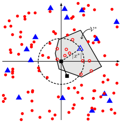
Figure 1: Random realization of the system model. APs and UEs are shown as triangle and circle markers, respectively. The typical node in this example is also a UE shown as a square. The shaded polygon area indicates the Voronoi guard region $\mathcal{V}^{*}$ within which no node (indicated by open marker) transmits. All nodes outside $\mathcal{V}^{*}$ (filled markers) generate interference that is experienced by the receiver of interest whose position ($x_{R})$ is indicated by an open diamond marker. This scenario may correspond to a (cross-cell) D2D link between typical node and receiver or to the receiver acting as relay aiding the donwlink or uplink communication of the typical node with its nearest AP.

The above model is general enough so that, by appropriately choosing $x_{R}$ and/or $x^{*}$, $I_{x_{R},a}$ and $I_{x_{R},u}$ correspond to many practical instances of (cross-mode) interference experienced in D2D/FD-enabled as well as conventional cellular networks. For example, for the case where $x^{*}\neq x_{R}\neq o$, Eq. (1) may correspond to the AP- and UE-generated interference power experienced by the receiver of a, potentially cross-cell, D2D link between the typical nodes at $o$ and $x_{R}$. Various other scenarios of practical interest are captured by the model, some of which are described in Table I. Note that from the scenarios identified in Table I, only the standard downlink and uplink scenarios have been considered previously in the literature [15, 16, 17, 25], however, without consideration of cross-mode interference, i.e., UE-generated and AP-generated interference for downlink and uplink transmissions, respectively. Reference [19] considers the UE-generated cross-mode interference experienced at the typical node in downlink mode, however, the results provided cannot not be straightforwardly generalized to the general case.

TABLE I: Special Cases of System Model

condition	scenario
$x_{R}\neq x^{*}$, $x^{*}\neq o$	General case. Corresponds to (a) a D2D link when the typical node sends data to the receiver or (b) to a relay-assisted cellular communication where the receiver acts a relay for the link between the typical node and it nearest AP (either downlink or uplink). The receiver is not guaranteed to lie within $\mathcal{V}^{*}$.
$x_{R}=o$, $x^{*}\neq o$	Typical node is a UE in receive mode and lies within $\mathcal{V}^{*}$. Represents a standard downlink when the nearest AP is transmitting data to the typical node/receiver.
$x_{R}=x^{*}$, $x^{*}\neq o$	Nearest AP to the typical node is in receive mode with the typical node lying in $\mathcal{V}^{*}$. Represents a standard uplink when the AP receives data from the typical node.
$x_{R}\neq o$, $x^{*}=o$	Typical node is an AP. When the typical node/AP is the one transmitting to the receiver, a non-standard downlink is established as $x_{R}$ is not necessarily lying within $\mathcal{V}^{*}$.
$x_{R}=x^{*}$, $x^{*}=o$	Typical node is an AP in receive mode; the position of the corresponding transmitter is unspecified and may as well lie outside $\mathcal{V}^{*}$, thus modeling a non-standard uplink.

For characterization of the performance of the communication link as well as obtaining insights on the effectiveness of the guard region $\mathcal{V}^{*}$ for reducing interference, it is of interest to describe the statistical properties of the random variables $I_{x_{R},a}$ and $I_{x_{R},u}$ . This is the topic of the following section, where the marginal statistics of $I_{x_{R},a}$ and $I_{x_{R},u}$ conditioned on $x^{*}$ and treating $x_{R}$ as a given, but otherwise free, parameter, are investigated in detail. Characterization of the joint distribution of $I_{x_{R},a}$ and $I_{x_{R},u}$ is left for future work.

Note that the respective unconditional interference statistics can be simply obtained by averaging over the distribution of $x^{*}$, which corresponds to a uniformly distributed $\angle x^{*}$ and a Rayleigh distributed $|x^{*}|$ of mean $1/(2\sqrt{\lambda_{a}})$ [27]. However, results conditioned on $x^{*}$ are also of importance on their own as they can serve as the mathematical basis for (optimal) resource allocation algorithms given network topology information, e.g., decide on whether the typical node employs D2D or cellular mode given knowledge of $x^{*}$.

For tractability purposes, the following assumption on the statistics of $\Phi_{u}$ will be considered throughout the analysis.

Assumption.

The positions of the (potentially) interfering UEs, $\Phi_{u}$, is a realization of an HPPP of density $\lambda_{u}>0$, that is independent of the positions of the APs, typical node, and receiver.

Remark: In general, this assumption is not exact since resource allocation and scheduling decisions over the entire network affect the distribution of interfering UE positions. For example, in the conventional uplink scenario with at least one UE per cell, the transmitting UE positions correspond to a VPLP process of density equal to $\lambda_{u}=\lambda_{a}$ [17, 19]. However, as also shown in [17, 19] for the standard uplink scenario, the HPPP assumption of the UE point process allows for a tractable, yet accurate approximation of the actual performance, which, as will be demonstrated in Sec. V, is also the case for other operational scenarios as well. For generality purposes, an arbitrary value $\lambda_{u}\neq\lambda_{a}$ is also allowed in the analysis, which can actually the case, e.g., in ultra dense networks with at most one UE allowed to transmit per cell, resulting in $\lambda_{u}<\lambda_{a}$ [26], and also serves as an approximate model for the case when some arbitrary/undefined coordination scheme is employed by other cells in the system (if at all), that may as well result in $\lambda_{u}>\lambda_{a}$.

III Interference Characterization

Towards obtaining a tractable characterization of the distribution of the (AP or UE) interference power, or, equivalently, its Laplace transform, the following standard result in PPP theory is first recalled [27].

Lemma 1.

Let $I\triangleq\sum_{x\in\tilde{\Phi}}Ph_{x}|x-z|^{-\alpha},z\in\mathbb{R}^{2}$, $P>0$, with $\tilde{\Phi}$ an inhomogeneous PPP of density $\lambda:\mathbb{R}^{2}\rightarrow[0,\infty)$, and $\{h_{x}\}_{x\in\Phi}$ i.i.d. exponential random variables of mean $1$. The Laplace transform of $I$ equals

$$\mathcal{L}_{I}(s) =\exp\left\{-\int_{\mathbb{R}^{2}}\lambda(x)\gamma(sP|x-z|^{-\alpha})dx\right\}$$ (2)

$$=\exp\left\{-2\pi\int_{0}^{\infty}\lambda_{z}(r)r\gamma(sPr^{-\alpha})dr\right\},$$ (3)

where $\gamma(t)\triangleq 1-\frac{1}{1+t}$, and the second equality holds only in the case of a circularly-symmetric density function w.r.t. point $z$, i.e., $\lambda(z+x)=\lambda_{z}(|x|)$, for an appropriately defined function $\lambda_{z}:[0,\infty)\rightarrow[0,\infty)$.

The above result provides a complete statistical characterization in integral form of the interference experienced at a position $z\in\mathbb{R}^{2}$ due to Poisson distributed interferers. Of particular interest is the case of a circularly-symmetric density, which only requires a single integration over the radial coordinate and has previously led to tractable analysis for various wireless network models of interest such as mobile ad hoc [1] and downlink cellular [25]. In the following, it will be shown that even though the interference model of Sec. II suggests a non circularly-symmetric interference density due to the random shape of the guard region, the Laplace transform formula of (3) holds exact for $I_{x_{R},a}$ and is a (tight) lower bound for $I_{x_{R},u}$ with appropriately defined circularly-symmetric equivalent density functions.

III-A AP-Generated Interference

Note that considering the Voronoi cell of a random AP at $x\in\Phi_{a}$ acting as a guard region has no effect on the distribution of the interfering APs. This is because the Voronoi cell of any AP is a (deterministic) function of $\Phi_{a}$, therefore, it does not impose any constraints on the realization of $\Phi_{a}$, apart from implying that the AP at $x$ does not produce interference. By well known properties of HPPPs [27], conditioning on the position $x$ of the non-interfering AP, has no effect on the distribution of the interfering APs. That is, the interfering AP positions are still distributed as an HPPP of density $\lambda_{a}$ as in the case without imposing any guard region whatsoever.

However, when it is the Voronoi cell of the nearest AP to the origin that is considered as a guard region, an implicit guard region w.r.t. AP-generated interference is formed. Indeed, the interfering APs, given the AP at $x^{*}$ is not interfering, are effectively distributed as an inhomogeneous PPP with density [25]

$$\tilde{\lambda}_{a}(x)=\lambda_{a}\mathbb{I}(x\notin\mathcal{B}(o,|x^{*}|)),x\in\mathbb{R}^{2},$$ (4)

i.e., an implicit circular guard zone is introduced around the typical node (see Fig. 1), since, if this was not the case, another AP could be positioned at a distance smaller than $|x^{*}|$ from the origin, which is impossible by assumption. This observation may be used to obtain the Laplace transform of the AP-generated interference experienced at $x_{R}$ directly from the formula of (2). However, the following result shows that the two-dimensional integration can be avoided as the formula of (3) is also valid in this case with an appropriately defined equivalent density function.

Proposition 2.

The Laplace transform, $\mathcal{L}_{I_{x_{R},a}}(s\mid x^{*})\triangleq\mathbb{E}(e^{-sI_{x_{R},a}}\mid x^{*})$, of the AP-generated interference power $I_{x_{R},a}$, conditioned on $x^{*}$, equals the right-hand side of (3) with $P=P_{a}$, $\alpha=\alpha_{a}$ and $\lambda_{z}(r)=\lambda_{x_{R},a}(r),r\geq 0$, where

$$\lambda_{x_{R},a}(r)\triangleq\begin{cases}\lambda_{a}&,r>|x^{*}|+|x_{R}|\\ \begin{cases}0&,|x^{*}|>|x_{R}|,\\ \lambda_{a}&,|x^{*}|<|x_{R}|,\end{cases}&,r\leq\left||x^{*}|-|x_{R}|\right|\\ \lambda_{a}/2&,|x^{*}|=|x_{R}|\\ \lambda_{a}\left(1-\frac{1}{\pi}\arccos\left(d\right)\right)&,\text{\emph{otherwise}},\end{cases}$$ (5)

with $d\triangleq\frac{r^{2}-(|x^{*}|^{2}-|x_{R}|^{2})}{2r|x_{R}|}$, for $x_{R}\neq o$, and

$$\lambda_{x_{R},a}(r)=\lambda_{a}\mathbb{I}(r\geq|x^{*}|),$$ (6)

for $x_{R}=o$.

Proof:

See Appendix A. ∎

The following remarks can be made:

1. The interference power experienced at an arbitrary position $x_{R}\neq o$ under the considered guard region scheme is equal in distribution to the interference power experienced at the origin without any guard region and with interferers distributed as an inhomogeneous PPP of an equivalent, $x_{R}$-depednent density given by (5).

2. Even though derivation of the statistics of $I_{x_{R},a}$ was conditioned on $x_{R}$ and $x^{*}$, the resulting equivalent inteferer density depends only on their norms $|x_{R}|$ and $|x^{*}|$. Although the indepedence from $\angle x^{*}$ might have been expected due to the isotropic property of $\Phi_{a}$ [1], there is no obvious reason why one would expect independence also from $\angle x_{R}$.

3. $\lambda_{x_{R},a}(r)$ is a decreasing function of $|x^{*}|$, corresponding to a (statistically) smaller AP interference power due to an increased guard zone area.

4. For $x_{R}=o$, corresponding to a standard downlink with interference generated from other donwlink transmissions, Prop. 2 coincides with the analysis of [25], as expected.

5. The Laplace transform of the interference in the case of $x_{R}\neq x^{*}\neq o$ was examined previously in [28]. However, the corresponding formulas appear as two-dimensional integrals that offer limited insights compared to the simpler and more intuitive equivalent density formulation given in Prop. 2.

6. The case $x_{R}=x^{*}\neq o$ corresponds to the nearest-neighbor transmission scenario considered in [29] where the validity of $\lambda_{x_{R},a}(r)$ in (5) as an equivalent density function for computation of the Laplace transform of the interference power was not observed.

7. In [30], the Laplace transform of the interference power experienced at $x_{R}\in\mathbb{R}^{2}$ due to a Poisson hole process, i.e., with interferers distributed as an HPPP over $\mathbb{R}^{2}$ except in the area covered by randomly positioned disks (holes), was considered. The holes were assumed to not include $x_{R}$ and a lower bound for the Laplace transform was obtained by considering only a single hole [30, Lemma 5], which coincides with the result of Prop. 2. This is not surprising as the positions of the APs, conditioned on $x^{*}$, are essentially distributed a single-hole Poisson process. Note that Prop. 2 generalizes [30, Lemma 5] by allowing $x_{R}$ to be covered by the hole and considers a different proof methodology.

Figure 2 shows the normalized density function $\lambda_{x_{R},a}(r)/\lambda_{a}$ for various values of $|x_{R}|$ and assuming that $|x^{*}|=1/(2\sqrt{\lambda_{a}})$, the expected distance from the nearest AP. It can be seen that the presence of the implicit circular guard region results in reducing the equivalent interferer density in certain intervals of the radial coordinate $r$, depending on the value of $|x_{R}|$. In particular, when $|x_{R}|<|x^{*}|$, it is guaranteed that no APs exist within a radius $|x^{*}|-|x_{R}|>0$ from $x_{R}$. In contrast, when $|x_{R}|>|x^{*}|$ there is no protection from APs in the close vicinity of $x_{R}$.

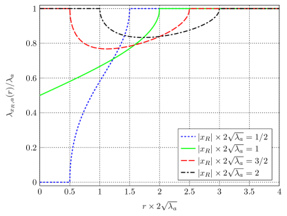
Figure 2: Equivalent radial density of interfering APs experienced at various $x_{R}\in\mathbb{R}^{2}$ , conditioned on $|x^{*}|=1/(2\sqrt{\lambda_{a}})$.

The case $|x_{R}|=|x^{*}|$ is particularly interesting since it corresponds to the case when the receiver is the AP at $x^{*}$, experiencing interference from other AP, e.g., when operating in FD. For $x^{*}\neq o$, corresponding to an uplink transmission by the typical node to its nearest AP, it can be easily shown that it holds

$$\lambda_{x^{*},a}(r)=\lambda_{a}\left(\frac{1}{2}+\frac{r}{2\pi|x^{*}|}\right)+\mathcal{O}(r^{3}),r\rightarrow 0,$$ (7)

i.e., the guard region results in the serving AP experiencing about half of the total interfering APs density in its close vicinity, which is intuitive as for asymptotically small distances from $x^{*}$ the boundary of the circular guard region in (4) can be locally approximated as a line that divides the plane in two halves, one with interferer density $\lambda_{a}$ and one with interferer density $0$. Figure 3 shows the normalized $\lambda_{x^{*},a}(r)$ for various values of $|x^{*}|$, where its linear asymptotic behavior as well as the advantage of a larger $|x^{*}|$ are clearly visible.

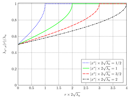
Figure 3: Equivalent radial density of interfering APs experienced at $x^{*}$.

III-B UE-Generated Interference

The positions of interfering UEs, conditioned on the realization of $\Phi_{a}$, are distributed as an inhomogeneous PPP of density

$$\tilde{\lambda}_{u}(x|\Phi_{a})=\lambda_{u}\mathbb{I}(x\notin\mathcal{V}^{*}),x\in\mathbb{R}^{2}.$$ (8)

Although the expression for $\tilde{\lambda}_{u}$ is very similar to the that of the density $\tilde{\lambda}_{a}$ of interfering APs given in (4), the random Voronoi guard region $\mathcal{V}^{*}$ appearing in (8) is significantly more complicated than the deterministic circular guard zone $\mathcal{B}(o,|x^{*}|)$, which renders the analysis more challenging. To simplify the following exposition, it will be assumed that a rotation of the Cartesian coordinate axes is performed such that $\angle x^{*}=0$. Note that this rotation has no effect in the analysis due to the isotropic property of the HPPP [1] and immediately renders the following results independent of the value of $\angle x^{*}$ in the original coordinate system.

Since it is of interest to examine the UE interference statistics conditioned only on $x^{*}$, a natural quantity to consider, that will be also of importance in the interference statistics analysis, is the probabilistic cell area (PCA) function $p_{c}(x\mid x^{*}),x\in\mathbb{R}^{2}$. This function gives the probability that a point $x\in\mathbb{R}^{2}$ lies within $\mathcal{V}^{*}$ conditioned only on $x^{*}$, i.e.,

$$p_{c}(x\mid x^{*}) \triangleq\mathbb{\mathbb{P}}(x\in\mathcal{V}^{*}\mid x^{*}).$$

Lemma 3.

For all $x\in\mathbb{R}^{2}$, the PCA function equals

$$p_{c}(x\mid x^{*})=\begin{cases}1&,|x|\leq|x^{*}|,\angle x=0,\\ e^{-\lambda_{a}|\mathcal{A}|}<1&,\text{\emph{otherwise}},\end{cases}$$

where $\mathcal{A}\triangleq\mathcal{B}(x,|x-x^{*}|)\setminus\mathcal{B}(o,|x^{*}|)$. For all $x\neq x^{*}$, it holds

$$|\mathcal{A}|\!=\!\begin{cases}r_{*}^{2}(|\angle x|\!+\!\theta_{*})\!-\!|x^{*}|^{2}|\angle x|\!+\!|x||x^{*}|\sin(|\angle x|)\!&,x^{*}\neq o,\\ \pi|x|^{2}\negmedspace&,x^{*}=o,\end{cases}$$

with $r_{*}\triangleq|x-x^{*}|=\sqrt{|x|^{2}+|x^{*}|^{2}-2|x||x^{*}|\cos(\angle x)}$ and

$$\theta_{*}\triangleq\begin{cases}\pi-\arcsin\left(\frac{|x|\sin(|\angle x|)}{r_{*}}\right)&,|x|\cos(\angle x)>|x^{*}|,\\ \arcsin\left(\frac{|x|\sin(|\angle x|)}{r_{*}}\right)&,|x|\cos(\angle x)\leq|x^{*}|.\end{cases}$$

Proof:

The probability that the point $x\in\mathbb{R}^{2}$ belongs to $\mathcal{V}^{*}$ is equal to the probability that there does not exist a point of $\Phi_{a}\setminus\{x^{*}\}$ within the set $\mathcal{A}$, which equals $e^{-\lambda_{a}\pi|\mathcal{A}|}$ [27]. For $|x|\leq|x^{*}|$ and $\angle x=0$, it is a simple geometrical observation that $\mathcal{A}=\textrm{\O}$, therefore, $|\mathcal{A}|=0$. When $x^{*}=o$, $\mathcal{A}=\mathcal{B}(x,|x|)\setminus\mathcal{B}(o,0)=\mathcal{B}(x,|x|)$, and, therefore, $|\mathcal{A}|=\pi|x|^{2}$. For all other cases, $|\mathcal{A}|$ can be computed by the same approach as in the proof of [31, Theorem 1]. The procedure is straightforward but tedious and is omitted. ∎

A simple lower bound for $p_{c}(x\mid x^{*})$ directly follows by noting that $\mathcal{A}\subseteq\mathcal{B}(x,|x-x^{*}|)$ for all $x\in\mathbb{R}^{2}$.

Corollary 4.

The PCA function is lower bounded as

$$p_{c}(x\mid x^{*})\geq e^{-\lambda_{a}\pi|x-x^{*}|^{2}},x\in\mathbb{R}^{2},$$ (9)

with equality if and only if $x^{*}=o$.

Remark: The right-hand side of (9) equals the probability that $x$ belongs to the Voronoi cell of the AP positioned at $x^{*}$ when the latter is not conditioned on being the closest AP to the origin or any other point in $\mathbb{R}^{2}$.

Figure 4 depicts $p_{c}(x\mid x^{*})$ for the case where $|x^{*}|=1/\sqrt{\lambda_{a}}$ (behavior is similar for other values of $|x^{*}|>0$). Note that, unless $x^{*}=o$, $p_{c}(x\mid x^{*})$ is not circularly symmetric w.r.t. any point in $\mathbb{R}^{2}$, with its form suggesting that points isotropically distributed in the vicinity of $x^{*}$ are more probable to lie within $\mathcal{V}^{*}$ than points isotropically distributed in the vicinity of $o$.

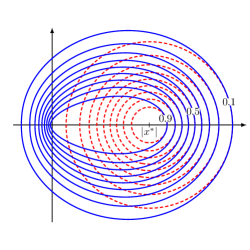
Figure 4: Contours of $p_{c}(x\mid x^{*})$ (solid lines), corresponding to probabilities $0.1$ to $0.9$ in steps of $0.1$, for $|x^{*}|=1/\sqrt{\lambda_{a}}$. The points of the line segment joining $o$ to $x^{*}$ are the only ones with $p_{c}(x|x^{*})=1$. The corresponding contours of $e^{-\lambda_{a}\pi|x-x^{*}|^{2}}$ are also shown (dashed lines).

The lower bound $e^{-\lambda_{a}\pi|x-x^{*}|^{2}},x\in\mathbb{R}^{2}$, is also shown in Fig. 4, clearly indicating the probabilistic expansion effect of the Voronoi cell of an AP, when the latter is conditioned on being the closest to the origin. This cell expansion effect is also demonstrated in Fig. 5 where the conditional average cell area, equal to

$$\mathbb{E}(|\mathcal{V}^{*}|\mid x^{*}) =\mathbb{E}\left(\left.\int_{\mathbb{R}^{2}}\mathbb{I}(x\in\mathcal{V}^{*})dx\right|x^{*}\right)$$

$$=\int_{\mathbb{R}^{2}}p_{c}(x|x^{*})dx,$$ (10)

is plotted as a function of the distance $|x^{*}|$, with the integral of (10) evaluated numerically using Lemma 3. Simulation results are also depicted serving as a verification of the validity of Lemma 3. It can be seen that the average area of the guard region increases with $|x^{*}|$, which implies a corresponding increase of the average number of UEs that lie within the region. However, as will be discussed in the following, even though resulting in more UEs silenced on average, an increasing $|x^{*}|$ does not necessarily imply improved protection from UE interference, depending on the receiver position.

The interference statistics of the UE-generated interference power are given in the following result.

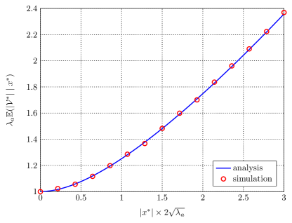
Figure 5: Average area of $\mathcal{V}^{*}$ conditioned on $x^{*}$ as a function of the (normalized) distance of $x^{*}$ from the origin.

Proposition 5.

The Laplace transform $\mathcal{L}_{I_{x_{R},u}}(s\mid x^{*})\triangleq\mathbb{E}(e^{-sI_{x_{R},u}}\mid x^{*})$ of the UE-generated interference power $I_{x_{R},u}$, conditioned on $x^{*}$, is lower bounded as the right-hand side of (3) with $P=P_{u}$, $\alpha=\alpha_{u}$ and $\lambda_{z}(r)=\lambda_{x_{R},u}(r),r\geq 0$, where

$$\lambda_{x_{R},u}(r)\triangleq\lambda_{u}\left(1-\frac{1}{2\pi}\int_{0}^{2\pi}p_{c}\left((r,\theta)+x_{R}\mid x^{*}\right)d\theta\right),$$ (11)

with $p_{c}(x\mid x^{*})$ as given in Lemma 3.

Proof:

See Appendix B. ∎

The following remarks can be made:

1. The statistics of the interfering UE point process when averaged over $\mathcal{V}^{*}$ (equivalently, over $\Phi_{a}\setminus\{x^{*}\}$) do not correspond to a PPP, even though this is the case when a fixed realization of $\mathcal{V}^{*}$ is considered. Therefore, it cannot be expected that Lemma 1 applies for $\mathcal{L}_{I_{x_{R},u}}(s\mid x^{*})$. However, as Prop. 5 shows, when the interfering point process is treated in the analysis as an PPP of an appropriately defined equivalent density function $\lambda_{x_{R},u}(r)$, a tractable lower bound for $\mathcal{L}_{I_{x_{R},u}}(s\mid x^{*})$ is obtained, which will be shown to be tight in the numerical results section.

2. For $x^{*}\neq o$, the non circularly-symmetric form of the PCA function results in an integral-form expression for the equivalent density $\lambda_{x_{R},u}(r)$ that depends in general on $\angle x_{R}$, in contrast to the case for $\lambda_{x_{R},a}(r)$ (see Sec. III.A, Remark 2). A closed form expression for the equivalent density is only available for $x^{*}=o$ discussed below.

3. When the receiver position is specified as $|x_{R}|\angle x_{R}$ with $\angle x_{R}$ uniformly distributed over $[-\pi,\pi)$, a straightforward extension of the proof of Prop. 5 results in the same lower bound for the conditioned Laplace transform of $I_{x_{R},u}$ as in Prop. 5, with $\lambda_{x_{R},u}(r)$ replaced by

   $$\lambda_{|x_{R}|,u}(r)\triangleq\frac{1}{2\pi}\int_{-\pi}^{\pi}\lambda_{x_{R},u}(r)d\angle x_{R},$$ (12)

   which is independent of $\angle x_{R}$.

Although $\lambda_{x_{R},u}(r)$ is not available in closed form when $x^{*}\neq o$, the numerical integration over a circular contour required in (11) is very simple. With $\lambda_{x_{R},u}(r),r\geq 0$, pre-computed, evaluation of the lower bound for $\mathcal{L}_{I_{x_{R},u}}(s\mid x^{*})$ is of the same (small) numerical complexity as the evaluation of $\mathcal{L}_{I_{x_{R},a}}(s\mid x^{*})$. Moreover, a closed-form upper bound for $\lambda_{x_{R},u}(r)$ is available, which can in turn be used to obtain a looser lower bound for $\mathcal{L}_{I_{x_{R},u}}(s\mid x^{*})$ that is independent of $\angle x_{R}$. The bound is tight in the sense that it corresponds to the exact equivalent density when $x^{*}=o$.

Proposition 6.

The equivalent density $\lambda_{x_{R},u}(r)$ of Prop. 5 is upper bounded as

$$\lambda_{x_{R},u}(r)\leq\lambda_{u}\left[1-e^{-\lambda_{a}\pi(|x^{*}|^{2}+|x_{R}|^{2}+r^{2})}\mathcal{I}_{0}(\lambda_{a}2\pi\bar{x}r)\right],$$ (13)

where $\bar{x}\triangleq\max(|x^{*}|,|x_{R}|)$ and $\mathcal{I}_{0}(\cdot)$ denotes the zero-order modified Bessel function of the first kind. Equality holds only when $x^{*}=o$.

Proof:

See Appendix C. ∎

An immediate observation of the above result is that, given $x_{R}$, the equivalent interfering UE density decreases for any $x^{*}\neq o$ compared to the case $x^{*}=o$. This behavior is expected due to the cell expansion effect described before. However, as the bound of (13) is independent on $\angle x_{R}$, it does not offer clear information on how the interferering UE density changes when different values of $x^{*}\neq o$ are considered for a given $x_{R}$. In order to obtain futher insights on the UE-generated interference properties, $\lambda_{x_{R},u}(r)$ is investigated in detail in the following section for certain special instances of $x_{R}$ and/or $x^{*}$, which are of particular interest in cellular networks.

IV Analysis of Special Cases of UE-Generated Interference

IV-A $x_{R}=x^{*}$

This case corresponds to a standard uplink cellular transmission with nearest AP association, no intra-cell interference, and interference generated by UEs outside $\mathcal{V}^{*}$ operating in uplink and/or D2D mode. This case was previously investigated in [16, 17] for $\lambda_{u}=\lambda_{a}$, with heuristically introduced equivalent densities averaged over $x^{*}$ (i.e., these densities are not expected to be valid for an arbitrary value of $x^{*}$). In this section, a more detailed investigation of the equivalent density properties is provided.

For this case, a tighter upper bound than the one in Prop. 6 is available for $\lambda_{x^{*},u}(r)$, which, interestingly, is independent of $|x^{*}|$, in the practical case when $x^{*}\neq o$.

Lemma 7.

For $x_{R}=x^{*}$, the equivalent density $\lambda_{x_{R},u}(r)=\lambda_{x^{*},u}(r)$ of Prop. 5 is upper bounded as

$$\lambda_{x^{*},u}(r)\leq\lambda_{u}\left(1-e^{-\lambda_{a}\pi r^{2}}\right),$$ (14)

with equality if and only if $x^{*}=o$.

Proof:

Follows by replacing the term $p_{c}\left((r,\theta)+x_{R}\mid x^{*}\right)=p_{c}\left((r,\theta)+x^{*}\mid x^{*}\right)$ appearing in (11) with its bound given in Cor. 4, which evaluates to $e^{-\lambda_{a}\pi r^{2}}$. ∎

The bound of (14) indicates that $\lambda_{x^{*},u}(r)$ tends to zero at least as fast as $\mathcal{O}(r^{2})$ for $r\rightarrow 0$, irrespective of $x^{*}$. The following exact statement on the asymptotic behavior of $\lambda_{x^{*},u}(r)$ shows that $\lambda_{x^{*},u}(r)\sim cr^{2},r\rightarrow 0$, with the value of $c$ independent of $|x^{*}|$ when $x^{*}\neq o$.

Proposition 8.

For $x_{R}=x^{*}$, the equivalent density $\lambda_{x_{R},u}(r)=\lambda_{x^{*},u}(r)$ of Prop. 5 equals

$$\lambda_{x^{*},u}(r)=\lambda_{u}\lambda_{a}b\pi r^{2}+\mathcal{O}(r^{3}),r\rightarrow 0,$$ (15)

with $b=1$ for $x^{*}=o$ and $b=1/2$ for $x^{*}\neq o$.

Proof:

For $x^{*}=o$, the result follows directly from Lemma 7. For $x^{*}\neq o$, it can be shown by algebraic manipulation based on Lemma 3, that the term $p_{c}\left((r,\theta)+x_{R}\mid x^{*}\right)=p_{c}\left((r,\theta)+x^{*}\mid x^{*}\right)$ appearing in (11) equals

$$\lambda_{u}\lambda_{a}\left(q\pi+(-1)^{q}\arccos(\sin(\theta))+\cos(\theta)\sin(\theta)\right)r^{2}+\mathcal{O}(r^{3}),$$

for $r\rightarrow 0$, where $q=0$ for $\theta\in[-\pi,-\pi/2]\cup[\pi/2,\pi)$ and $q=1$ for $\theta\in(-\pi/2,\pi/2)$. Substituting this expression in (11) and performing the integration leads to the result. ∎

Equation (15) indicates that imposing a guard region $\mathcal{V}^{*}$ when $x^{*}\neq o$ reduces the interfering UE density by half in the close vicinity of $x^{*}$, compared to the case $x^{*}=o$. This effect is similar to the behavior of $\lambda_{x^{*},a}(r)$ discussed in Sec. III. A. However, $\lambda_{x^{*},a}(0)=\lambda_{a}/2$ , whereas $\lambda_{x^{*},u}(0)=0$, clearly demonstrating the effectiveness of the guard region for reducing UE-generated interference in the vicinity of $x^{*}$.

For non-asymptotic values of $r$, the behavior of $\lambda_{x^{*},u}(r)$ can only be examined by numerical evaluation of (11). Figure 6 depicts the normalized equivalent density $\lambda_{x^{*},u}(r)/\lambda_{u}$ for various values of $|x^{*}|$ in the range of practical interest $[0,3/(2\sqrt{\lambda_{a}})]$ (note that $\mathbb{P}(|x^{*}|>3/(2\sqrt{\lambda_{a}}))=e^{-\lambda_{a}\pi\left(3/(2\sqrt{\lambda_{a}})\right)^{2}}\approx 8.5\times 10^{-4})$. It can be seen that for non-asymptotic values of $r$, $\lambda_{x^{*},u}(r)$ is a decreasing function of $|x^{*}|$ for all $r>0$, corresponding to a reduced UE-generated interference. This is expected since, as evident from Fig. 4, the cell expansion effect with increasing $|x^{*}|$ can only improve the interference protection at $x^{*}$.

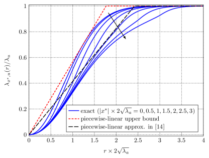
Figure 6: Equivalent density function $\lambda_{x^{*},u}(r)$ for various $|x^{*}|$ (solid curves), with the direction of the arrow corresponding to increasing $|x^{*}|$. A piecewise-linear approximation and bound are also shown.

Interestingly, the dependence of $\lambda_{x^{*},u}(r)$ on $|x^{*}|$, although existing, can be seen to be rather small. This observation, along with Prop. 8, strongly motivates the consideration of a single curve as an approximation to the family of curves in Fig. 6. A natural approach is to consider the upper bound of (14), which has the benefit of being available in closed form. This is essentially the approach that was heuristically employed in [17] without observing that it actually corresponds to a (tight) bound for the equivalent interferer density.

Another approach is to consider a piecewise-linear curve, which, in addition to having a simple closed form, results in a closed form approximate expression for the bound of $\mathcal{L}_{I_{x^{*},u}}(s\mid x^{*})$ as given below (details are straightforward and omitted).

Lemma 9.

With the piecewise-linear approximation

$$\lambda_{x^{*},u}(r)\approx\lambda_{u}\min\left(\delta r,1\right),r\geq 0,$$ (16)

for some $\delta>0$, the lower bound for $\mathcal{L}_{I_{x^{*},u}}(s\mid x^{*})$ equals

$$\exp\left\{-\lambda_{u}\pi\left[C(P_{u}s)^{2/\alpha}+\frac{1}{\delta^{2}}\left(\frac{2}{3}\tilde{F}\left(3\right)-\tilde{F}\left(2\right)\right)\right]\right\}$$

where $C\triangleq(2\pi/\alpha)/\sin(2\pi/\alpha)$ and $\tilde{F}(x)\triangleq{}_{2}F_{1}\left(1,\frac{x}{\alpha},1+\frac{x}{\alpha},\frac{-1}{sP_{u}\delta^{\alpha}}\right)$ with ${}_{2}F_{1}\left(\cdot\right)$ denoting the hypergeometric function.

A piecewise-linear approximation as in (16) was heuristically proposed in [16] for a slightly more general system model than the one considered here. A closed form formula for $\delta$ was provided, only justified as obtained by means of curve fitting without providing any details on the procedure. For the system model considered in this paper, this formula results in $\delta\approx 0.82687\sqrt{\lambda_{a}}$ and the corresponding piecewise-linear approximation of the equivalent density is also depicted in Fig. 6. It can be seen that this approximation is essentially an attempt to capture the average behavior of $\lambda_{x^{*},u}(r)$ over $|x^{*}|$, thus explaining its good performance reported in [16]. However, it is not clear why this particular value of $\delta$ is more preferable than any other (slightly) different value. A more rigorous approach for the selection of $\delta$ is to consider the tightest piecewise-linear upper bound for $\lambda_{x^{*},u}(r)$, which leads to another (looser) lower bound for $\mathcal{L}_{I_{x_{R},u}}(s\mid x^{*})$. This bound corresponds to a value of $\delta\approx 1.13118\sqrt{\lambda_{a}}$ , found by numerical optimization, and is also shown in Fig. 6.

Remark: In [19], the case $x_{R}=x^{*}=o$ with VPLP distributed interferering UEs of density $\lambda_{u}=\lambda_{a}$ is considered. It is shown that the resulting interference properties, averaged over $x^{*}$, are approximately similar to the properties of the interference generated by PPP distributed interferers of an equivalent density $\lambda_{a}(1-e^{-\frac{12}{5}\lambda_{a}\pi r^{2}})=\frac{12}{5}\lambda_{a}^{2}\pi r^{2}+\mathcal{O}(r^{3})$. It is noted that, in the asymptotic ($r\rightarrow 0$) regime, the equivalent density of Prop. 8 is smaller but has the same scaling order. This suggest that the analysis of this section is a reasonable approximation also for the VPLP case. This is verified numerically in Sec. V.

IV-B $x^{*}=o$

This case corresponds to the typical node being an AP, i.e., a typical AP. Note that, in contrast to the cases when $x^{*}\neq o$, the Voronoi cell of the typical AP is not conditioned to cover any point in $\mathbb{R}^{2}$, therefore, no cell expansion effect is observed and, for $x_{R}\neq o$, it is possible that the receiver lies outside the guard region. Note that when it is the typical node/AP that is transmitting to the receiver, the resulting operational scenario is different from the standard downlink with nearest AP association [25] where the receiver lies within the Voronoi cell of the serving AP by default. This scenario may arise, for example, in case of D2D communications, where both communicating UEs receive data (e.g., control information) from the same AP.

The equivalent interfering UE density is given in Prop. 6 and is depicted in Fig. 7 for various values of $|x_{R}|$. Note that the case $x_{R}=o$ corresponds to the typical AP in receive mode, whereas for $x_{R}\neq o$ the typical AP transmits. It can be seen that increasing $|x_{R}|$ effectively results in reduced protection in the close vicinity of the receiver since the latter is more probable to lie near the edge or even outside the Voronoi guard region.

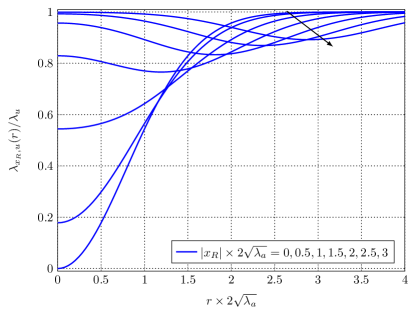
Figure 7: Equivalent density function $\lambda_{x_{R},u}(r)$ when $x^{*}=o$ with the direction of the arrow corresponding to increasing values of $|x_{R}|$.

IV-C $x_{R}=o$

This case corresponds to the typical node being at receive mode. One interesting scenario which corresponds to this case is downlink cellular transmission with nearest AP association, where interference is due to transmitting UEs (e.g., in uplink or D2D mode) that lie outside the serving cell.

When $x^{*}=o$, the setup matches the case $x_{R}=x^{*}$ with $x^{*}=o$, discussed above, and it holds $\lambda_{o,u}(r|x^{*})=\lambda_{u}\left(1-e^{-\lambda_{a}\pi r^{2}}\right)$. For $x^{*}\neq o$, the asymptotic behavior of $\lambda_{o,u}(r|x^{*})$ can be obtained by the same approach as in the proof of Prop. 8.

Proposition 10.

For $x^{*}\neq o$ the equivalent density function $\lambda_{x_{R},u}(r)=\lambda_{o,u}(r|x^{*})$ of Prop. 5 equals

$$\lambda_{o,u}(r)=\lambda_{u}\lambda_{a}\frac{8}{\pi}|x^{*}|r+\mathcal{O}(r^{2}),r\rightarrow 0.$$

In stark contrast to the behavior of $\lambda_{x^{*},u}(r)$, $\lambda_{o,u}(r)$ tends to $0$ only linearly (instead of quadradically) as $r\rightarrow 0$ when $x^{*}\neq o$, and with a rate that is also proportional to (instead of independent of) $|x^{*}|$. This implies that the typical node is not as well protected from interfering UEs as its nearest AP, experiencing an increased equivalent interferer density in its close vicinity as $|x^{*}|$ increases. This can be understood by noting that with increasing $|x^{*}|$, the origin, although contained in a guard region of (statistically) increasing area, is more probable to lie near the cell edge (Fig. 1 demonstrates such a case.)

The strong dependence of $\lambda_{o,u}(r)$ on $|x^{*}|$ observed for $r\rightarrow 0$ also holds for all values of $r$. This is shown in Fig. 8 where the numerically evaluated $\lambda_{o,u}(r)$ is depicted for the same values of $|x^{*}|$ as those considered in Fig. 6. It can be seen that $\lambda_{o,u}(r)$ increases with $|x^{*}|$ for all $r$ up to approximately $1-1.5$ times the average value of $|x^{*}|$ (equal to $1/(2\sqrt{\lambda_{a}})$), whereas it decreases with $|x^{*}|$ for greater $r$ .

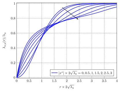
Figure 8: Equivalent density function $\lambda_{o,u}(r)$ for various $|x^{*}|$, with the direction of the arrow corresponding to increasing $|x^{*}|$.

This behavior of $\lambda_{o,u}(r)$, especially for $r\rightarrow 0$, does not permit the use of single function to be used as a reasonable approximation or bound for $\lambda_{o,u}(r)$, irrespective of $|x^{*}|$, as was done for the case for $\lambda_{x^{*},u}(r)$. Noting that the upper bound of (13) has the same value whenever $|x^{*}|$ or $|x_{R}|$ are zero, it follows that the curves shown in Fig. 7 with $|x_{R}|$ replaced by $|x^{*}|$ are upper bounds for the corresponding curves of Fig. 8. Unfortunately, it can be seen that the bound is very loose for small $r$ and/or large $|x^{*}|$.

Remark: In [19], the case $x_{R}=o$ with VPLP distributed interferering UEs of density $\lambda_{u}=\lambda_{a}$ is considered. It is shown that the resulting interference properties, averaged over $x^{*}$, are approximately similar to the properties of the interference generated by PPP distributed interferers of (equivalent) density $\lambda_{a}(1-e^{-\frac{9}{4}\sqrt{\lambda_{a}}\pi r}+\frac{1}{2}r^{2}e^{-\frac{5}{4}\lambda r^{2}})=\frac{9}{4}\lambda_{a}^{3/2}\pi r+\mathcal{O}(r^{2})$. As an approximation of this case, the equivalent density of Prop. 10 can be averaged over $|x^{*}|$ resulting in $\frac{4}{\pi}\lambda_{a}^{3/2}\pi r+\mathcal{O}(r^{2})$. It can be seen that the approximation is able to capture the asymptotic scaling of the actual density, even though with a slightly smaller factor, suggesting the validity of the analysis as a reasonable approximation for this case as well.

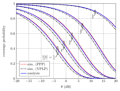
(a)

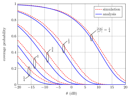
(b)

Figure 9: Coverage probability of the link between the typical node and an isotropically positioned receiver under UE interference for (a) $\lambda_{u}=\lambda_{a}$, (b) $\lambda_{u}=10\lambda_{a}$.

IV-D $|x_{R}|\in(0,|x^{*}|),\angle x_{R}=0$

The previous cases demonstrate how different the properties of the UE-generated interference become when different receiver positions are considered. This observation motivates the question of which receiver position is best protected from UE interference given the positions $o$ and $x^{*}\neq o$ of the typical node and nearest AP, respectively. This question is relevant in, e.g., relay-aided cellular networks where the communication between a UE and its nearest AP is aided by another node (e.g., an inactive UE) [32]. Although the performance of a relay-aided communication depends on multiple factors including the distances among the nodes involved and considered transmission scheme [33], a reasonable choice for the relay position is the one experiencing less interference.

By symmetry of the system geometry, this position should lie on the line segment joining the origin with $x^{*}$ (inclusive). However, as can be seen from Figs. 6 and 8, the shape of the equivalent interferer density does not allow for a natural ordering of the different values of $x_{R}$. For example, $\lambda_{x^{*},u}(r)$ is smaller than $\lambda_{o,u}(r)$ for small $r$, whereas the converse holds for large $r$. Noting that the receiver performance is mostly affected by nearby generated interference [1], a natural criterion to order the interfering UE densities for varying $x_{R}$ is their asymptotic behavior as $r\rightarrow 0$. For $|x_{R}|=|x^{*}|$ and $|x_{R}|=o$, this is given in Props. 8 and 10, respectively. For all other positions the asymptotic density is given by the following result.

Proposition 11.

For $|x_{R}|\in(0,|x^{*}|),\angle x_{R}=0$, and $x^{*}\neq o$, the equivalent density function $\lambda_{x_{R},u}(r)$ of Prop. 5 equals

$$\lambda_{x_{R},u}(r)=\lambda_{u}\lambda_{a}\frac{8}{9\pi}\frac{(|x^{*}|/|x_{R}|)^{2}}{|x^{*}|-|x_{R}|}r^{3}+\mathcal{O}(r^{4}),r\rightarrow 0.$$ (17)

It follows that the optimal receiver position must have $|x_{R}|\in(0,|x^{*}|)$ since, in this case, the density scales as $\mathcal{O}(r^{3})$ instead of $\mathcal{O}(r)$ and $\mathcal{O}(r^{2})$ when $|x_{R}|=0$ and $|x_{R}|=|x^{*}|$, respectively. Its value can be easily obtained by minimization of the expression in (17) w.r.t. $|x_{R}|$.

Corollary 12.

The receiver position that experiences the smallest equivalent UE interferer density in its close vicinity lies on the line segment joining the origin to $x^{*}$ and is at distance $|x^{*}|/\sqrt{2}$ from the origin. The corresponding equivalent density equals $\lambda_{x_{R},u}(r)=\lambda_{u}\lambda_{a}\frac{32}{9\pi}r^{3}+\mathcal{O}(r^{4}),r\rightarrow 0$.

V Numerical Examples

In this section, numerical examples will be given, demonstrating the performance of various operational scenarios in cellular networks that can be modeled as special cases of the analysis presented in the previous sections. The system performance metric that will be considered is $\mathcal{L}_{I_{x_{R},k}}(\rho^{\alpha_{k}}\theta|x^{*})$, with $k\in\{a,u\}$ depending on whether AP- or UE-generated interference is considered, with $\rho>0$, $\theta>0$ given. Note that this metric corresponds to the coverage probability that the signal-to-interference ratio (SIR) at $x_{R}$ is greater than $\theta$, when the distance between transmitter and receiver is $\rho$, the direct link experiences a path loss exponent $a_{k}$ and Rayleigh fading, and the transmit power is equal to $P_{k}$ [1]. For simplicity and w.l.o.g., all the following examples correspond to $\lambda_{a}=1$ and $\alpha_{a}=\alpha_{u}=4$.

The analytical results of the previous sections will be compared against simulated system performance where, in a single experiment, the distribution of interfering APs and UEs is generated as follows. Given the AP position closest to the origin, $x^{*}$, the interfering AP positions are obtained as a realization of a PPP of density as in (4). Afterwards, an independent realization of a HPPP of density $\lambda_{u}$ is generated, which, after removing the points lying within $\mathcal{V}^{*}$, represents the interferering UE positions.

In addition, for cases where the UE-generated interference is of interest, a VPLP process of density $\lambda_{u}=\lambda_{a}$ is also simulated, corresponding to scenarios where one UE from each Voronoi cell in the system transmits (as in the standard uplink scenario with nearest AP association).

V-A D2D Link not Necessarily Contained in a Single Cell

In this example, UE-generated inteference is considered at a receiver position $x_{R}\neq o$ with $\angle x_{R}$ uniformly distributed in $[-\pi,\pi)$ and $\rho=|x_{R}|$. This case may model a D2D link where the typical node is a UE that directly transmits to a receiver isotropically distributed at a distance $|x_{R}|>0$ . A guard region $\mathcal{V}^{*}$ is established by the closest AP to the typical node, however, it is not guaranteed to include $x_{R}$, i.e., the D2D nodes may not be contained within the same cell, which is a common scenario that arises in practice, referred to as cross-cell D2D communication [21].

With interference generated from other UEs in D2D and/or uplink mode, a lower bound for $\mathcal{L}_{I_{x_{R},u}}(\rho^{\alpha_{u}}\theta|x^{*})$ can be obtained using Prop. 5 with an equivalent density function $\lambda_{|x_{R}|,u}(r)$ as given in (12). Figure 9 shows this lower bound for $\lambda_{u}=\lambda_{a}$ (Fig. 9a) and $\lambda_{u}=10\lambda_{a}$ (Fig. 9b). The position $x^{*}$ is assumed to be isotropically distributed with $|x^{*}|=1/(2\sqrt{\lambda_{a}})$ and various values of the ratio $|x_{R}|/|x^{*}|$ are considered. It can be seen that, compared to the simulation under the PPP interference assumption, the quality of the analytical lower bound depends on $\lambda_{u}$. For $\lambda_{u}=\lambda_{a}$, it is very close to the exact coverage probability, whereas for $\lambda_{u}=10\lambda_{a}$, it is reasonably tight and able to capture the behavior of the exact coverage probability over varying $|x_{R}|$. Also, for $\lambda_{u}=\lambda_{a}$ and a VPLP interference, the analytical expression provides a reasonably accurate approximation for the performance of this analytically intractable case. As expected, performance degradation is observed with increasing $|x_{R}|$, due to both increasing path loss of the direct link as well as increased probability of the receiver lying outside $\mathcal{V}^{*}$.

V-B AP-to-D2D-Receiver Link

In this example, AP-generated inteference is considered at a receiver position $x_{R}\neq o$ with $\angle x_{R}$ uniformly distributed in $[-\pi,\pi)$ and $\rho=|x^{*}-x_{R}|$. This case is similar to the previous, however, considering AP-generated interference and the receiver at $x_{R}$ receiving data from the AP node at $x^{*}$. This case models the scenario where the typical node establishes a D2D connection with a node at $x_{R}$, and the AP at $x^{*}$ sends data to $x_{R}$ via a dedicated cellular link (e.g., for control purposes or for implementing a cooperative transmission scheme). Note that, in contrast to the previous case, the link distance $\rho$ is random and equal to $\rho=|x^{*}|+|x_{R}|-2|x^{*}||x_{R}|\cos\psi$, with $\psi$ uniformly distributed in $[-\pi,\pi)$. The exact coverage probability of this link can be obtained using Prop. 2 followed by a numerically computed expectation over $\psi$.

Figure 10 shows $\mathbb{E}(\mathcal{L}_{I_{x_{R},a}}(\rho^{\alpha_{a}}\theta|x^{*}))$ for an isotropically distributed $x^{*}$ with $|x^{*}|=1/(2\sqrt{\lambda_{a}})$, and for various values of the ratio $|x_{R}|/|x^{*}|$. Note that the case $|x_{R}|=0$ corresponds to the standard downlink transmission model with nearest AP association [25]. Monte Carlo evaluation of the coverage probability (not shown here) perfectly matches the analytical curves. It can be seen that increasing $|x_{R}|$ reduces the coverage probability for small SIR but increases it for high SIR. This is in direct proportion to the behavior of the equivalent interferer density $\lambda_{x_{R},a}(r)$ with increasing $|x_{R}|$ shown in Fig. 2.

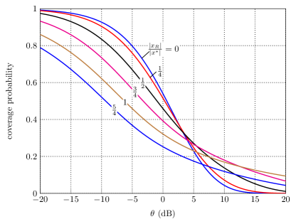
Figure 10: Coverage probability for the link between the AP positioned at $x^{*}$ ($|x^{*}|=1/(2\sqrt{\lambda_{a}})$) and an isotropicaly positioned receiver.

V-C Uplink with Nearest AP Association

In this example, UE-generated interference is considered at a receiver position $x_{R}=x^{*}$ with $\rho=|x^{*}|$ and $\lambda_{u}=\lambda_{a}$ corresponding to the conventional uplink transmission scenario with nearest AP association and one active UE per cell (no cross-mode interference). Figure 11 shows the lower bound of $\mathcal{L}_{I_{x_{R},u}}(\rho^{\alpha_{u}}\theta|x^{*})$ obtained by Prop. 5 as well as the looser, but more easily computable, lower bound obtained using the closed form expression given in Lemma 7 with $\delta=1.13118\sqrt{\lambda_{a}}$ (resulting in the tightest bound possible with a piecewise-linear equivalent density function). The coverage probability is computed for an AP at a distance $|x^{*}|$=$c/(2\sqrt{\lambda_{a}})$ from the typical node with $c=1/2,1,2$, roughly corresponding to a small, average, and large uplink distance (performance is independent of $\angle x^{*}$).

As was the case in Fig. 9a, Prop. 5 provides a very tight lower bound for the actual coverage probability (under the PPP model for the interfering UE positions). The bound of Lemma 7, although looser, is nevertheless a reasonable approximation of the performance, especially for smaller values of $|x^{*}|$. Compared to the VPLP model, the PPP model provides an optimistic performance prediction that is, however, reasonably tight, especially for large $|x^{*}|$. This observation motivates its usage as a tractable approximation of the actual inteference statistics as was also reported in [16, 17]. Interestingly, the bound of Lemma 7 happens to provide an even better approximation for the VPLP performance for $|x^{*}|$ close to or smaller than $1/(2\sqrt{\lambda_{a}})$.

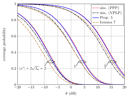
Figure 11: Coverage probability of the uplink between the typical node its nearest AP ($\lambda_{u}=\lambda_{a}$).

V-D Effect of Guard Region on UE-Generated Interference Protection

In order to see the effectiveness of a Voronoi guard region for enhancing link quality under UE-generated interference, the performance under the following operational cases is examined.

• Case A (no guard region is imposed): This results in the standard transmission model under an HPPP of interferers positions of density $\lambda_{u}$ [1]. The exact coverage probability is well known (see, e.g., [1, Eq. 3.29]).

• Case B (transmitter imposes a Voronoi guard region): This case corresponds to $x^{*}=o$, $x_{R}\neq o$, modeling an non-standard downlink transmission (see also description in Table I).

• Case C (receiver imposes a Voronoi guard region): This case corresponds to $x_{R}=x^{*}=o$ modeling an non-standard uplink transmission (see also description in Table I)

Cases B and C correspond to the analysis considered in Sec. V. B. Assuming the same link distance $\rho$ for all cases, Fig. 12 shows the analytically obtained coverage probability (exact for Case A, lower bound for Cases B and C), assuming $\lambda_{u}=\lambda_{a}$. It can be seen that imposing a Voronoi guard region (Cases B and C) is always beneficial, as expected. However, for large link distances, Case B provides only marginal gain as the receiver is very likely to be located at the edge or even outside the guard region. In contrast, the receiver is always guaranteed to be protected under case C, resulting in the best performance and significant gains for large link distances.

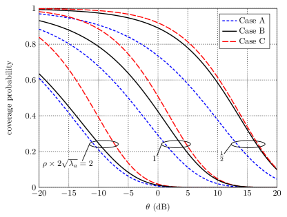
Figure 12: Coverage probability under UE interference for the links corresponding to the cases described in Sec. V. D.

VI Conclusion

This paper considered the analytical characterization of cross-mode inter-cell interference experienced in future cellular networks. By employing a stochastic geometry framework, tractable expressions for the interference statistics were obtained that are exact in the case of AP-generated interference and serve as a tight lower bound in the case of UE-generated interference. These expressions are based on appropriately defined equivalent interferer densities, which provide an intuitive quantity for obtaining insights on how the interference properties change according to the type of interference and receiver position. The considered system model and analysis are general enough to capture many operational scenarios of cellular networks, including conventional downlink/uplink transmissions with nearest AP association as well as D2D transmissions between UEs that do not necessarily lie in the same cell. The analytical expressions of this paper can be used for sophisticated design of critical system aspects such as mode selection and resource allocation towards getting the most out D2D- and/or FD-enabled cellular communications. Interesting topics for future research is investigation of the joint properties of AP- and UE-generated interference, consideration of different transmit powers for uplink and D2D UE transmissions, as well as extension of the analysis to the case of heterogeneous, multi-tier networks.

Appendix A Proof of Proposition 2

Let $\tilde{\Phi}_{a}\triangleq\Phi_{a}\setminus\{x^{*}\}$ denote the interfering AP point process. Given $x^{*}$, $\tilde{\Phi}_{a}$ is an inhomogeneous PPP of density $\tilde{\lambda}_{a}(x),x\in\mathbb{R}^{2}$, defined in (4). Density $\tilde{\lambda}_{a}(x)$ is circularly symmetric w.r.t. $x_{R}=o$, which, using Lemma 1, directly leads to the Laplace transform expression of (3) with radial density as in (6). Considering the case $x_{R}\neq o$, it directly follows from Lemma 1 and (2) that

$$\mathcal{L}_{I_{x_{R},a}}(s) =\exp\left\{-\int_{\mathbb{R}^{2}}\tilde{\lambda}_{a}(x+x_{R})\gamma(sP_{a}|x|^{-\alpha_{a}})dx\right\}$$

by a change of integration variable. By switching to polar coordinates (centered at $o$) for the integration, the right-hand side of (3) results with $P=P_{a}$, $\alpha=\alpha_{a}$ and $\lambda_{x_{R}}(r)=\lambda_{x_{R},a}(r)$, where

$$\lambda_{x_{R},a}(r) =\frac{1}{2\pi}\int_{0}^{2\pi}\tilde{\lambda}_{a}((r,\theta)+x_{R})d\theta$$

$$=\frac{\lambda_{a}}{2\pi}\int_{0}^{2\pi}\mathbb{I}\left\{(r,\theta)+x_{R}\notin\mathcal{B}(o,|x^{*}|)\right\}d\theta$$

$$=\frac{\lambda_{a}}{2\pi}\int_{0}^{2\pi}\mathbb{I}\left\{(r,\theta)\notin\mathcal{B}(-x_{R},|x^{*}|)\right\}d\theta$$

$$=\frac{\lambda_{a}}{2\pi}\int_{0}^{2\pi}\mathbb{I}\left\{(r,\theta)\notin\mathcal{B}((|x_{R}|,0),|x^{*}|)\right\}d\theta,$$

with $x_{R}$ representing the polar coordinates of the receiver in the first equality, with a slight abuse of notation. The last equality follows by noting that the integral does not depend on the value of $\angle x_{R}$. Evaluation of the final integral is essentially the evaluation of an angle (see Fig. 13), which can be easily obtained by elementary Euclidean geometry, resulting in the expression of (5).

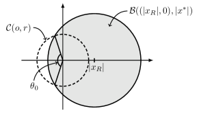
Figure 13: Geometrical figure depicting the angle $\theta_{0}$, which is equal to quantity $\int_{0}^{2\pi}\mathbb{I}\left((r,\theta)\notin\mathcal{B}((|x_{R}|,0),|x^{*}|)\right)d\theta$ appearing in the proof of Prop. 2.

Appendix B Proof of Proposition 5

It holds

$$\mathcal{L}_{I_{x_{R},u}}(s\mid x^{*})$$

$$= \mathbb{E}\left(\mathbb{E}\left(e^{-sI_{x_{R},u}}\mid\Phi_{a}\right)\mid x^{*}\right)$$

$$\stackrel{{\scriptstyle(a)}}{{=}} \mathbb{E}\left(\left.\exp\left\{-\int_{\mathbb{R}^{2}}\tilde{\lambda}_{u}(x|\Phi_{a})\gamma(sP_{u}|x-x_{R}|^{-\alpha_{u}})dx\right\}\right|x^{*}\right)$$

$$\geq \exp\left\{-\int_{\mathbb{R}^{2}}\mathbb{E}\left(\tilde{\lambda}_{u}(x+x_{R}|\Phi_{a})\mid x^{*}\right)\gamma(sP_{u}|x|^{-\alpha_{u}})dx\right\},$$

where $(a)$ follows by noting that, conditioned on $\Phi_{a}$, the interfering UE point process equals $\Phi_{u}\setminus\mathcal{V}^{*}$, which is distributed as an inhomogeneous PPP of density $\tilde{\lambda}_{u}(x|\Phi_{1}),x\in\mathbb{R}^{2}$ as given in (8), and using Lemma 1. The inequality is an application of Jensen’s inequality with a change of integration variable. Result follows by noting that $\mathbb{E}\left(\tilde{\lambda}_{u}(x|\Phi_{a})\mid x^{*}\right)=\lambda_{u}\left[1-p_{c}(x\mid x^{*})\right]$ and switching to polar coordinates for the integration.

Appendix C Proof of Proposition 6

Replacing the PCA function in (11) with its lower bound as per Cor. 4 results in the equivalent density bound

$$\lambda_{x_{R},u}(r)$$

$$\leq \lambda_{u}\left(1-\frac{1}{2\pi}\int_{0}^{2\pi}e^{-\lambda_{a}\pi|(r,\theta)+x_{R}-x^{*}|^{2}}d\theta\right)$$

$$\stackrel{{\scriptstyle(a)}}{{\leq}} \lambda_{u}\left(1-\frac{e^{-\lambda_{a}\pi|x^{*}|^{2}}}{2\pi}\int_{0}^{2\pi}e^{-\lambda_{a}\pi|(r,\theta)+x_{R}|^{2}}d\theta\right)$$

$$\stackrel{{\scriptstyle(b)}}{{=}} \lambda_{u}\left(1-\frac{e^{-\lambda_{a}\pi|x^{*}|^{2}}}{2\pi}\int_{0}^{2\pi}e^{-\lambda_{a}\pi|(r,\theta)+(|x_{R}|,0)|^{2}}d\theta\right)$$

$$\stackrel{{\scriptstyle(c)}}{{=}} \lambda_{u}\left(1-\frac{e^{-\lambda_{a}\pi(|x^{*}|^{2}+|x_{R}|^{2}+r^{2})}}{2\pi}\int_{0}^{2\pi}e^{\lambda_{a}\pi 2r|x_{R}|\cos\theta}d\theta\right),$$

where $(a)$ follows by application of the triangle inequality, $(b)$ by noting that the integral is independent of $\angle x_{R}$ and $(c)$ since $|(r,\theta)+(|x_{R}|,0)|^{2}=r^{2}+|x_{R}|^{2}-2r|x_{R}|\cos(\pi-\theta)$ (cosine law). The integral in the last equation is equal to $2\pi\mathcal{I}_{0}(\lambda_{a}2\pi|x_{R}|r)$. By exchanging the roles $x^{*}$ and $x_{R}$ in $(a)$ and following the same reasoning, another upper bound of the form of $(c)$ results, with the only difference that the integrand has $|x^{*}|$ instead of $|x_{R}|$ and evaluates to $2\pi\mathcal{I}_{0}(\lambda_{a}2\pi|x^{*}|r)$. Considering the minimum of these two bounds leads to (13).

References

- [1] M. Haenggi and R. K. Ganti, “Interference in Large Wireless Networks,” Found. Trends Netw., vol. 3, no. 2, pp. 127–248, 2008.
- [2] F. Boccardi, R. W. Heath, A. Lozano, T. L. Marzetta, and P. Popovski, “Five disruptive technology directions for 5G,” IEEE Commun. Mag., vol. 52, pp. 74–80, Feb. 2014.
- [3] K. Doppler, M. Rinne, C. Wijting, C. Ribeiro, and K. Hugl, “Device-to-Device Communication as an Underlay to LTE-Advanced Networks,” IEEE Commun. Mag., vol. 50, no. 3, pp. 170–177, Mar. 2012.
- [4] A. Sabharwal, P. Schniter, D. Guo, D. Bliss, S. Rangarajan, and R. Wich- man, “In-band full-duplex wireless: Challenges and opportunities,” IEEE J. Select. Areas Commun., vol. 32, pp. 1637–1652, Sept. 2014.
- [5] L. Lei and Z. Zhong, “Operator controlled device-to-device communications in LTE-Advanced networks,” IEEE Wireless Commun., vol. 19, no. 3, pp. 96–104, Jun. 2012.
- [6] M. Haenggi, J. G. Andrews, F. Baccelli, O. Dousse, and M. Franceschetti, “Stochastic geometry and random graphs for the analysis and design of wireless networks,” IEEE J. Select. Areas Commun., vol. 27, pp. 1029-1046, Sept. 2009.
- [7] Q. Ye, M. Al-Shalash, C. Caramanis, and J. G. Andrews, “Resource optimization in device-to-device cellular systems using time-frequency hopping,” IEEE Trans. Wireless Commun., vol. 13, no. 10, pp. 5467–5480, Oct. 2014.
- [8] X. Lin, J. G. Andrews, and A. Ghosh, “Spectrum sharing for device-to-device communication in cellular networks,” IEEE Trans. Wireless Commun., vol. 13, no. 12, pp. 6727–6740, Dec. 2014.
- [9] N. Lee, X. Lin, J. G. Andrews, and R. W. Heath, Jr., “Power control for D2D underlaid cellular networks: Modeling, algorithms and analysis,” IEEE J. Sel. Areas Commun., vol. 33, no. 1, pp. 1–13, Jan. 2015.
- [10] S. Stefanatos, A. Gotsis, and A. Alexiou, “Operational region of D2D communications for enhancing cellular network performance,” IEEE Trans. Wireless Commun., vol. 14, no. 11, pp. 5984–5997, Nov. 2015.
- [11] A. Hasan and J. G. Andrews, “The guard zone in wireless ad hoc networks,” IEEE Trans. Wireless Commun., vol. 6, no.3, pp. 897–906, Mar. 2007.
- [12] G. George, R. K. Mungara, and A. Lozano, “An Analytical Framework for Device-to-Device Communication in Cellular Networks,” IEEE Trans. Wireless Commun., vol. 14, no. 11, pp. 6297–6310, Nov. 2015.
- [13] Z. Chen and M. Kountouris, “Decentralized opportunistic access for D2D underlaid cellular networks,” Jul. 2016. [Online]. Available: http://arxiv.org/abs/1607.05543.
- [14] J. G. Andrews, R. K. Ganti, N. Jindal, M. Haenggi, and S. Weber, “A primer on spatial modeling and analysis in wireless networks,” IEEE Commun. Mag., vol. 48, no. 11, pp. 156–163, Nov. 2010.
- [15] H. ElSawy and E. Hossain, “On stochastic geometry modeling of cellular uplink transmission with truncated channel inversion power control,” IEEE Trans. Wireless Commun., vol. 13, no. 8, pp. 4454–4469, Aug. 2014.
- [16] H. Lee, Y. Sang, and K. Kim, “On the uplink SIR distributions in heterogeneous cellular networks,” IEEE Commun. Lett., vol. 18, no. 12, pp. 2145–2148, Dec. 2014.
- [17] S. Singh, X. Zhang, and J. G. Andrews, “Joint rate and SINR coverage analysis for decoupled uplink-downlink biased cell associations in HetNets,” IEEE Trans. Wireless Commun., vol. 14, no. 10, pp. 5360–5373, Oct. 2015.
- [18] B. Błaszczyszyn and D. Yogeshwaran, “Clustering comparison of point processes with applications to random geometric models,” in Stochastic Geometry, Spatial Statistics and Random Fields, vol. 2120, Lecture Notes in Mathematics. Cham, Switzerland: Springer-Verlag, 2015, pp. 31–71.
- [19] M. Haenggi, “User point processes in cellular networks,” IEEE Wireless Commun. Lett., vol. 6, no. 2, pp. 258–261, Apr. 2017.
- [20] M. Di Renzo, W. Lu, and P. Guan, “The intensity matching approach: A tractable stochastic geometry approximation to system-level analysis of cellular networks,” IEEE Trans. Wireless Commun., vol. 15, no. 9, pp. 5963–5983, Sep. 2016.
- [21] H. Zhang, Y. Ji, L. Song, and H. Zhu “Hypergraph based resource allocation for cross-cell device-to-device communications,” in Proc. IEEE Int. Conf. Commun. (ICC), Kuala Lumpur, Malaysia, May 2016, pp. 1–6.
- [22] Z. Tong and M. Haenggi, “Throughput analysis for full-duplex wireless networks with imperfect self-interference cancellation,” IEEE Trans. Commun., vol. 63, no. 11, pp. 4490–4500, Nov. 2015.
- [23] C. Psomas, M. Mohammadi, I. Krikidis, and H. A. Suraweera, “Impact of directionality on interference mitigation in full-duplex cellular networks,” IEEE Trans. Wireless Commun., vol. 16, no. 1, pp. 487–502, Jan. 2017.
- [24] K. S. Ali, H. ElSawy, and M.-S. Alouini, “Modeling cellular networks with full-duplex D2D communication: a stochastic geometry approach,” IEEE Trans. Commun., vol. 64, no. 10, pp. 4409–4424, Oct. 2016.
- [25] J. G. Andrews, F. Baccelli, and R. K. Ganti, “A tractable approach to coverage and rate in cellular networks,” IEEE Trans. Commun., vol. 59, no. 11, pp. 3122–3134, Nov. 2011.
- [26] S. Stefanatos and A. Alexiou, “Access Point density and bandwidth partitioning in ultra-dense wireless networks,” IEEE Trans. Commun., vol. 62, no. 9, pp. 3376–3384, Sept. 2014.
- [27] F. Baccelli and B. Błaszczyszyn, Stochastic Geometry and Wireless Networks. Delft, The Netherlands: Now Publishers Inc., 2009.
- [28] Z. Chen and M. Kountouris, “Guard zone based D2D underlaid cellular networks with two-tier dependence,” 2015 IEEE International Conference on Communication Workshop (ICCW), London, 2015, pp. 222-227.
- [29] M. Haenggi, “The local delay in poisson networks,” IEEE Trans. Inf. Theory, vol. 59, pp. 1788–1802, Mar. 2013.
- [30] Z. Yazdanshenasan, H. S. Dhillon, M. Afshang, and P. H. J. Chong, “Poisson hole process: theory and applications to wireless networks,” IEEE Trans. Wireless Commun., vol. 15, no. 11, pp. 7531–7546, Nov. 2016.
- [31] S. Sadr and R. S. Adve, “Handoff rate and coverage analysis in multi-tier heterogeneous networks,” IEEE Trans. Wireless Commun., vol. 14, no. 5, pp. 2626–2638, May 2015.
- [32] H. E. Elkotby and M. Vu, “Uplink User-Assisted Relaying Deployment in Cellular Networks,” IEEE Trans. on Wireless Commun., vol. 14, no. 10, pp. 5468–5483, Oct. 2015.
- [33] A. E. Gamal and Y.-H. Kim, Network Information Theory, Cambridge University Press, 2012.