PyCaMa: Python for cash management

Abstract

Selecting the best policy to keep the balance between what a company holds in cash and what is placed in alternative investments is by no means straightforward. We here introduce PyCaMa, a Python module for multiobjective cash management based on linear programming that allows to derive optimal policies for cash management with multiple bank accounts in terms of both cost and risk of policies.

1 Motivation and significance

Cash managers usually deal with multiple banks to receive payments from customers and to send payments to suppliers. Operating such a cash management system implies a number of transactions between accounts, what is called a policy, to maintain the system in a safe state, meaning that there exists enough cash balance to face payments and avoid an overdraft. In addition, optimal policies allow to keep the sum of both transaction and holding costs at a minimum. However, cash managers may be interested not only in cost but also in the risk of policies. Hence, risk analysis can also be incorporated as an additional goal to be minimized in cash management. As a result, deriving optimal policies in terms of both cost and risk within systems with multiple bank accounts is not an easy task. To this end, we here introduce PyCaMa, a software tool to provide such optimal policies.

Despite the recent advances in cash management da Costa Moraes et al. (2015), there is a lack of supporting software to aid the transition from theory to practice. In order to fill this gap, we provide a cash management module in Python for practitioners interested in building decision support systems for cash management. In addition, this software allows to tackle open research questions such as: (i) managing multiple bank accounts Baccarin (2009); (ii) the impact of cash flow forecasting accuracy in the cost of policies Gormley and Meade (2007); Salas-Molina et al. (2017); (iii) the utility of different risk measures in cash management Salas-Molina et al. (2016); and (iv) robust optimization Soyster (1973); Ben-Tal and Nemirovski (2002).

In practice, cash management systems can be represented as a set of bank accounts and a set of transactions between them. These systems can be introduced in PyCaMa by means of an incidence matrix establishing the relationship between allowed transactions and bank accounts. Once a cash management system is defined, cash managers should describe the current cost structure including fixed and variable costs for each transaction, and holding costs for each bank account. If available, PyCaMa also accepts cash flow forecasts to reduce the uncertainty about the future Stone (1972); Gormley and Meade (2007). In addition, minimum balances for each account can be set for precautionary purposes. Finally, PyCaMa provides optimal policies for a given planning horizon by solving a linear program using a state-of-the-art mathematical programming solver such as Gurobi Gurobi Optimization, Inc (2016).

Summarizing, PyCaMa is a Python-Gurobi tool aimed to automate multiobjective decision making in cash management. To the best of our knowledge, PyCaMa is the first software tool to solve the multiobjective cash management problem with multiple bank accounts. PyCaMa contributes to support cash management decision-making: (i) by empowering cash managers to derive optimal cash policies within a real-world context in which cash management systems with multiple bank accounts are the rule rather than the exception; and (ii) by providing a computational finance framework that can be used either as a tool for empirical research or as a benchmarking for further research in cash management. Next, we describe the optimization problem that PyCaMa solves.

2 The cash management problem with multiple bank accounts

In order to formulate the problem, we first define a cash management system as a set of bank accounts and their relationship such as the one depicted in Figure 1. Any cash management system with $m$ bank accounts and $n$ allowed transactions can be represented by an $n\times m$ incidence matrix $A$, with element $a_{ij}=1$ if transaction $i$ adds cash to account $j$, $a_{ij}=-1$ if transaction $i$ removes cash from account $j$, and $a_{ij}=0$ when no transaction is allowed between accounts. In the usual case of linear transaction costs between accounts with a fixed part $\gamma_{0}$, and a variable part $\gamma_{1}$, the transaction cost function $\Gamma(\boldsymbol{x}_{t})$ at time $t$ is defined as:

$$\Gamma(\boldsymbol{x}_{t})=\boldsymbol{\gamma}_{0}^{T}\cdot\boldsymbol{z}_{t}+\boldsymbol{\gamma}_{1}^{T}\cdot\boldsymbol{x}_{t}$$ (1)

where $\boldsymbol{z}_{t}$ is an $n\times 1$ binary vector with element $z_{i}$ set to one if the $i$-th element of $\boldsymbol{x}_{t}$ is not null, and zero otherwise; $\boldsymbol{\gamma}_{0}$ is a $n\times 1$ vector of fixed transaction costs for each transaction; and $\boldsymbol{\gamma}_{1}$ is a $n\times 1$ vector of variable transaction costs. On the other hand, the expected holding cost function at time $t$ is usually expressed as:

$$H(\boldsymbol{\hat{b}}_{t})=\boldsymbol{v}^{T}\cdot\boldsymbol{\hat{b}}_{t}$$ (2)

where $\boldsymbol{v}$ is an $m\times 1$ column vector with the $j$-th element set to the holding cost per money unit for account $j$.

Figure 1: A cash management system with three accounts.

2.1 Single objective optimization: cost

Consider now a cash planning horizon of $\tau$ time steps, e.g., the next 5 working days. Within a single cost objective, given an initial cash balance $\boldsymbol{b}_{0}$, the solution to the problem, namely, the policy $X=\langle\boldsymbol{x}_{1},\boldsymbol{x}_{2},\ldots,\boldsymbol{x}_{\tau}\rangle$ that minimizes the sum of transaction and holding costs, up to the time step $\tau$, can be obtained by solving the following linear program:

$$\operatorname{min}\sum_{t=1}^{\tau}c(\boldsymbol{x}_{t})=\sum_{t=1}^{\tau}\left(\Gamma(\boldsymbol{x}_{t})+\boldsymbol{v}^{T}\cdot\boldsymbol{\hat{b}}_{t}\right)$$ (3)

subject to:

$$\boldsymbol{\hat{b}}_{t-1}+\boldsymbol{\hat{f}}_{t}+A^{T}\boldsymbol{x}_{t}=\boldsymbol{\hat{b}}_{t}$$ (4)

$$\boldsymbol{\hat{b}}_{t}\geq\boldsymbol{\hat{b}}_{min}$$ (5)

$$\boldsymbol{x}_{t}\in\mathbb{R}_{\geq 0}^{n}$$ (6)

$$t=1,2,\ldots,\tau$$ (7)

where $\boldsymbol{\hat{b}}_{t-1}$ and $\boldsymbol{\hat{b}}_{t}$ are $m\times 1$ vectors with previous and current balances for each account, respectively; $\boldsymbol{\hat{f}}_{t}$ is an $m\times 1$ vector with expected net cash flows for each account; and finally, $\boldsymbol{x}_{t}$ is an $n\times 1$ vector with the set of transactions (control actions) occurred at time $t$; and $\boldsymbol{\hat{b}}_{min}$ is a $m\times 1$ vector of minimum cash balances.

2.2 Multiobjective optimization: cost and risk

However, cash managers may also be interested in the risk of cash management policies Salas-Molina et al. (2016). Similarly to the definition of Conditional Value-at-Risk in Rockafellar and Uryasev (2002), we consider the Conditional Cost-at-Risk ($CCaR$) measure of policy $X$, which we define as the conditional excess expectation above a particular cost reference $c_{0}$ as follows:

$$CCaR(X,c)=E[c(\boldsymbol{x}_{t})|c(\boldsymbol{x}_{t})>c_{0}],\hskip 5.69054pt\forall\boldsymbol{x}_{t}\in X.$$ (8)

An additional advantage of $CCaR$ is that it is a coherent measure of risk in the sense of Artzner et al. (1999). Minimizing $CCaR$ is equivalent to minimize the sum of the positive deviation of cost above reference $c_{0}$. As a result, we next incorporate $CCaR$ as an additional goal to be optimized through the following multiobjective linear program in which cost-risk preferences are expressed by means of weights $w_{1}$ and $w_{2}$:

$$\operatorname{min}\hskip 5.69054pt\left[\frac{w_{1}}{C_{max}}\sum_{t=1}^{n}c(\boldsymbol{x}_{t})+\frac{w_{2}}{R_{max}}\sum_{t=1}^{n}\delta_{t}^{+}\right]$$ (9)

subject to:

$$\boldsymbol{\hat{b}}_{t-1}+\boldsymbol{\hat{f}}_{t}+A^{T}\boldsymbol{x}_{t}=\boldsymbol{\hat{b}}_{t}$$ (10)

$$\boldsymbol{\hat{b}}_{t}\geq\boldsymbol{\hat{b}}_{min}$$ (11)

$$c(\boldsymbol{x}_{t})-\delta_{t}^{+}\leq c_{0}$$ (12)

$$\sum_{t=1}^{n}c(\boldsymbol{x}_{t})\leq C_{max}$$ (13)

$$\sum_{t=1}^{n}\delta_{t}^{+}\leq R_{max}$$ (14)

$$\boldsymbol{x}_{t}\in\mathbb{R}_{\geq 0}^{n}$$ (15)

$$w_{1}+w_{2}=1$$ (16)

$$t=1,2,\ldots,\tau$$ (17)

where $\delta_{t}^{+}$ is an auxiliary variable used to measure deviations from a cost reference as in goal programming Aouni et al. (2014). $C_{max}$ and $R_{max}$ can be regarded as budget limitations for both cost and risk, leading to unfeasible policies when these constraints are no satisfied.

3 Software description

Since the cash management problem is an optimization problem, PyCaMa is based on linear programming to provide optimal policies. However, it is important to highlight that the linear programs described in Section 2.1 (only for cost) and in Section 2.2 (for both cost and risk) should be considered as baseline models that can be used for benchmarking purposes.

A cash management system, a cost structure and a set of minimum balances are sufficient to create an instance of the multibank class. It is assumed that cash managers are able to produce cash flow forecasts for each bank account as an additional input to the problem. Otherwise, forecasts must be set to zero. Next, given an initial condition and a set of cash flow forecasts for the immediate future, cash managers can derive optimal policies either in terms of only cost or in terms of both cost an risk.

3.1 Software architecture

PyCaMa is organized around the multibank class. An instance of this class is initialized by means of different data structures in Python such as: (i) a list of $m$ banks; (ii) a list of $n$ transactions; (iii) an $n\times m$ incidence matrix $A$, establishing the cash management system; (iv) two dictionaries linking transactions and both fixed ($\boldsymbol{\gamma}_{0}$) and variable ($\boldsymbol{\gamma}_{1}$) transaction costs; (v) a dictionary linking each bank account to holding costs in vector $\boldsymbol{v}$; (vi) a list with $m$ minimum cash balances in $\boldsymbol{\hat{b}}_{min}$; as follows:

⬇

1myproblem = multibank(banks, trans, A, g0, g1, v, b_min)

Once a multibank object is created, a number of methods are implemented to provide cash managers with useful functionalities that we next describe.

3.2 Software functionalities

Cash managers can retrieve the main characteristics of the cash management system they are dealing with by using function describe. All the input data is then shown for descriptive purposes. The main functionality of PyCaMa is function solvecost, which provides a solution (if any) for the linear program encoded by equations (3)-(7). Given a list of length $m$ with an initial condition $\boldsymbol{b}_{0}$, and a $\tau\times m$ matrix $F$ of forecasts (with elements set to zero if not available) obtained by concatenating vectors $\boldsymbol{\hat{f}}_{t}$ with $t$ ranging in $1,2,\ldots,\tau$, the optimal policy is obtained by executing:

⬇

1solution_1 = myproblem.solvecost(b0, F)

If the linear program has a feasible solution, function solvecost returns its optimal policy for each transaction and time step. Otherwise, solvecost warns the user that it was unable to find a solution. In addition, a $\tau\times n$ matrix with the optimal policy, and a $\tau\times m$ matrix with optimal balances derived from the last optimization can be retrieved by means of functions policy and balance, respectively, and the last objective value by calling the attribute objval of the multibank object.

Furthermore, cash managers interested in minimizing not only cost but also the risk of policies measured by the $CCaR$, can call the function solverisk, which provides a solution (if any) for the linear program encoded by equations (9)-(17), given $b_{0}$ and $F$, a cost reference $c_{0}$, $C_{max}$ and $R_{max}$ budget limitations, and weights $w_{1}$ and $w_{2}$, by executing:

⬇

1solution_2 = myproblem.solverisk(b0, F, c0, Cmax, Rmax, w1, w2)

Summarizing, the Python input and outputs of PyCaMa are shown in Table I.

Table I: Python inputs and outputs of PyCaMa

Inputs	Outputs	Function or attribute
List of banks	Description of the system	describe
List of transactions	Cost optimal policy list	solvecost
Incidence matrix	Cost-Risk optimal policy list	solverisk
Dictionary of transaction costs	Last optimal policy matrix	policy
Dictionary of holding costs	Last optimal balance matrix	balance
List of minimum balances	Last objective value	objval
Matrix of forecasts	Cost budget	costmax
List of initial cash balances	Risk budget	riskmax
Cost reference	Cost reference	costref
Cost and risk maximum budgets	Cost weight	costweight
Cost and risk weights	Risk weight	riskweight

4 An illustrative example

Consider again the cash management system of Figure 1 with two current bank accounts 1 and 2, and an investment account 3. Temporary idle cash balances can be invested in short-term marketable securities and bonds through an investment account 3 with an average return of 3.6% per annum, equivalent to 0.01% per day. This is equivalent to set a holding cost 0.01% per day for both accounts 1 and 2. Transactions are allowed between all three accounts and charged with fixed ($\gamma_{0}$) and variable ($\gamma_{1}$) costs determining the cost structure detailed in Table II.

Table II: Cost structure data for the example.

Transaction	$\gamma_{0}$ (€)	$\gamma_{1}$ (%)	Account	$v$ (%)
1	50	0	1	0.01
2	50	0	2	0.01
3	100	0.01	3	0
4	50	0.001
5	100	0.01
6	50	0.001

Assume also that a hypothetical cash manager can obtain forecasts with a maximum cumulative error of 2 million euros for a planning horizon of five days. As a result, she sets a minimum cash balance of 2 million for accounts 1 and 2. Given a initial cash balance $b_{0}=\left[5,8,12\right]$, for accounts 1, 2 and 3, she aims to derive the optimal policy for the next five days. To this end, let us assume that she obtains the next matrix of forecasts (with figures in millions of euros) by applying some predictive method as in Salas-Molina et al. (2017).

$$F=\left[\begin{array}[]{rrrrr}1&-3&0\\ 1&-9&0\\ 6&6&0\\ -1&4&0\\ -3&6&0\\ \end{array}\right].$$ (18)

An instance of the multibank class is created by introducing all the required input data as follows:

⬇

1from PyCaMa import * # Import module

2banks = [1, 2, 3] # Bank accounts

3trans = [1, 2, 3, 4, 5, 6] # Transactions

4g0 = {1:50, 2:50, 3:100, 4:50, 5:100, 6:50} # Fixed costs

5g1 = {1:0, 2:0, 3:100, 4:10, 5:100, 6:10} # Variable costs

6bmin = [2, 2, 0] # Minimum balances

7v = {1:100, 2:100, 3:0} # Holding costs

8A = np.array([[ 1, -1, 0, 0, 1, -1],

9 [-1, 1, 1, -1, 0, 0],

10 [ 0, 0, -1, 1, -1, 1]]).T # Incidence matrix

11myproblem = multibank(banks, trans, A, g0, g1, v, bmin)

Then, cash managers can derive the optimal policy by executing function $solvecost(b_{0},F)$:

⬇

1b0 = [5, 8, 12] # Initial balance

2F = np.array([[ 1, -3, 0], # Forecast matrix

3 [ 1, -9, 0],

4 [ 6, 6, 0],

5 [-1, -4, 0],

6 [-1, 6, 0]])

7solution_1 = myproblem.solvecost(b0, F) # Solution

A more compact representation of the optimal policy and balances can be obtained by calling functions policy and balance, which is ready to be visualized through common plotting commands in Python as shown in Figure 2. The same instance of the multibank class problem can now be solved in terms of cost and risk by setting a cost reference $c_{0}=3,000$ €, budget limits $C_{max}=5,000$ €, $R_{max}=5,000$ €, and weights $w_{1}=w_{2}=0.5$, and by executing $solverisk(b_{0},F,c_{0},C_{max},R_{max},w_{1},w_{2})$, resulting in a slightly different policy.

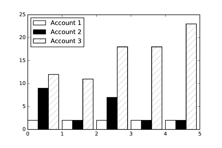
Figure 2: Optimal balances for the cost minimization example.

5 Impact

PyCaMa is a cash management tool that can be used either to automate decision-making in cash management or to support scientific discovery in the context of computational finance. More precisely, PyCaMa is a promising tool to tackle the following set of open research questions:

• The cash management problem with multiple bank accounts. There is a lack of research about multidimensional cash management systems with the exception of Baccarin (2009), who followed a rigorous theoretical approach. PyCaMa offers a suitable way to follow a more practical approach by providing support for research on actual-world scenarios.

• The impact of cash flow forecasting accuracy. Although the utility of forecasts in cash management was initially demonstrated by Gormley and Meade (2007) and confirmed by (Salas-Molina et al., 2017), both approaches were restricted to a single bank account. PyCaMa allows to extend this analysis to cash management systems with multiple bank accounts. As a result, PyCaMa represents a tool to find the best forecasting models and their potential benefits derived from improving predictive accuracy.

• The utility of different risk measures. A multiobjective approach to the cash management problem has been recently proposed in Salas-Molina et al. (2016) in which the risk of alternative policies is measured by the standard deviation of daily costs. The utility of alternative risk measures can be evaluated by easily extending PyCaMa to consider different risk measures.

• Robust optimization. Two robust approaches to optimization problems were proposed by Soyster (1973) and Ben-Tal and Nemirovski (2002) to deal with uncertainty. PyCaMa can be used to help researchers compare existing and new robust approaches to the cash management problem in terms of both cost and risk.

Moreover, under the realistic assumption of time-varying circumstances, cash managers and researchers are allowed to modify the cost structure to analyze to what extent a change in any of the parameters of the cost structure leads to different optimal policies and, ultimately, to a variation in the cost (and risk) of managing cash. It is also important to highlight that, since Miller and Orr (1966) different optimization models have been proposed based on a set of bounds. Determining such bounds may be problematic in practice due to the strong assumptions made on the probability distribution of cash flows. PyCaMa do not assume any particular form of the cash flow generating process allowing an unconstrained optimization procedure in the sense that no restriction is placed neither on the form of the policy nor on the distribution of cash flows. As a result, we expect that PyCaMa will be progressively adopted by cash managers and researchers as a more efficient tool to automate decision-making in cash management.

6 Conclusions

In this paper, we have introduced PyCaMa, a Python module for cost and risk multiobjective optimization within a context of cash management systems with multiple bank accounts. PyCaMa solves the cash management problem when it is formulated as a linear program that aims to minimize either only cost or both cost and risk of cash policies. PyCaMa is implemented through the Gurobi Python modeling environment as a powerful and flexible way to allow an easy integration of its functionality in a more general application. Through an illustrative example, we have shown the key features of PyCaMa, and we have demonstrated how PyCaMa allows users to model complex cash management systems in an intuitive manner transforming a graphical representation in an optimization model ready to find a solution and to further experimentation. We firmly believe that PyCaMa can be a helpful tool for academic research and financial decision-support software development in the field of short-term financial planning. Natural extensions of PyCaMa include the implementation of different forecasting techniques and additional measures of risk to be added to the current functionality.

References

- Aouni et al. (2014) Aouni, B., Colapinto, C., and La Torre, D. (2014). Financial portfolio management through the goal programming model: Current state-of-the-art. European Journal of Operational Research, 234(2):536–545.
- Artzner et al. (1999) Artzner, P., Delbaen, F., Eber, J.-M., and Heath, D. (1999). Coherent measures of risk. Mathematical finance, 9(3):203–228.
- Baccarin (2009) Baccarin, S. (2009). Optimal impulse control for a multidimensional cash management system with generalized cost functions. European Journal of Operational Research, 196(1):198–206.
- Ben-Tal and Nemirovski (2002) Ben-Tal, A. and Nemirovski, A. (2002). Robust optimization–methodology and applications. Mathematical Programming, 92(3):453–480.
- da Costa Moraes et al. (2015) da Costa Moraes, M. B., Nagano, M. S., and Sobreiro, V. A. (2015). Stochastic cash flow management models: A literature review since the 1980s. In Decision Models in Engineering and Management, pages 11–28. Springer International Publishing.
- Gormley and Meade (2007) Gormley, F. M. and Meade, N. (2007). The utility of cash flow forecasts in the management of corporate cash balances. European Journal of Operational Research, 182(2):923–935.
- Gurobi Optimization, Inc (2016) Gurobi Optimization, Inc (2016). Gurobi optimizer reference manual.
- Miller and Orr (1966) Miller, M. H. and Orr, D. (1966). A model of the demand for money by firms. The Quarterly journal of economics, pages 413–435.
- Rockafellar and Uryasev (2002) Rockafellar, R. T. and Uryasev, S. (2002). Conditional value-at-risk for general loss distributions. Journal of Banking and Finance, 26(7):1443–1471.
- Salas-Molina et al. (2017) Salas-Molina, F., Martin, F. J., Rodríguez-Aguilar, J. A., Serrà, J., and Arcos, J. L. (2017). Empowering cash managers to achieve cost savings by improving predictive accuracy. International Journal of Forecasting, 33(2):403–415.
- Salas-Molina et al. (2016) Salas-Molina, F., Pla-Santamaria, D., and Rodriguez-Aguilar, J. A. (2016). A multi-objective approach to the cash management problem. Annals of Operations Research, pages 1–15.
- Soyster (1973) Soyster, A. L. (1973). Technical note—convex programming with set-inclusive constraints and applications to inexact linear programming. Operations research, 21(5):1154–1157.
- Stone (1972) Stone, B. K. (1972). The use of forecasts and smoothing in control limit models for cash management. Financial Management, 1(1):72.