Non-Invertibility of spectral x-ray photon counting data with pileup

Abstract

In the Alvarez-Macovski method [R.E. Alvarez and A. Macovski, Phys. Med. Biol., 1976, 733-744], the attenuation coefficient is approximated as a linear combination of functions of energy multiplied by coefficients that depend on the material composition at points within the object. The method then computes the line integrals of the basis set coefficient from measurements with different x-ray spectra. This paper shows that the transformation from photon counting detector data with pileup to the line integrals can become ill-conditioned under some circumstances leading to highly increased noise.

Methods: An idealized model that includes pileup and quantum noise is used. The noise variance of the line integral estimates is computed using the Cramèr-Rao lower bound (CRLB). The CRLB is computed as a function of object thickness for photon counting detector data with three and four bin pulse height analysis (PHA) and low and high pileup.

Results: With four bin PHA data the transformation is well conditioned with either high or low pileup. With three bin PHA and high pileup, the transformation becomes ill-conditioned for specific values of object attenuation. At these values the CRLB variance increases by approximately $10^{5}$ compared with the four bin PHA or low pileup results. The condition number of the forward transformation matrix also shows a spike at those attenuation values.

Conclusion: Designers of systems using counting detectors should study the stability of the line integral estimator output with their data.

Key Words: photon counting, pileup, spectral x-ray, dual energy, spectral x-ray, energy selective, Cramèr-Rao lower bound

I INTRODUCTION

This paper studies the stability of the Alvarez-Macovski method[1] with x-ray photon counting data with pileup. The method uses an expansion of the x-ray attenuation coefficient as a linear combination of functions of energy multiplied by constants that depend only on the material composition at points in the object. Transmission measurements with multiple x-ray spectra are then used to estimate the line integrals of the basis set coefficients. With a photon counting detector, the transmitted photons are analyzed with pulse height analysis[2](PHA) so that each bin provides a separate measurement spectrum.

In order to focus on fundamental effects, the noise in the line integral estimates is computed using an idealized model that only includes pileup and quantum noise. In the computation, the transmitted spectra are first computed using realistic models of the x-ray tube source spectrum[3] and tabulated attenuation coefficients[4]. The recorded photon counts with pileup are then computed using a non-paralyzable model of the recorded photon counts with pileup[2]. In the model, the recorded energies are assumed to be the sum of the energies of the photons incident during the dead time period. The recorded energy data are measured using pulse height analysis with ideal rectangular energy bins. The PHA bin counts are the input data to the A-vector estimator.

The probability distribution of the PHA bin counts with pileup is modeled as multivariate normal with parameters that depend on the spectrum of the photons incident on the detector and the pileup parameter[5]. A universal limit on the A-vector estimate noise variance is computed using the Cramèr-Rao lower bound (CRLB), which is the minimum covariance for any unbiased estimator[6]. The CRLB is computed from the multivariate normal parameters[6] as a function of object thickness for photon counting detector data with three or four bin PHA with low and high pileup.

The results show that with high pileup three bin PHA data the noise variance exhibits a sharp peak at specific object thicknesses. The peak does not appear with four bin PHA data or three bin data with low pileup. The peak variance is approximately $10^{5}$ times the values for the same thicknesses in the cases without the instability.

II METHODS

II-A The Alvarez-Macovski method

For biological materials and an externally administered high atomic number contrast agent, we can approximate the x-ray attenuation coefficient $\mu(\mathbf{r},E)$ accurately with a three function basis set[7]

$$\mu(\mathbf{r},E)=a_{1}(\mathbf{r})f_{1}(E)+a_{2}(\mathbf{r})f_{2}(E)+a_{3}(\mathbf{r})f_{3}(E).$$ (1)

In this equation, $a_{i}(\mathbf{r})$ are the basis set coefficients and $f_{i}(E)$ are the basis functions, $i=1\ldots 3$. As implied by the notation, the coefficients $a_{i}(\mathbf{r})$ are functions only of the position $\mathbf{r}$ within the object and the functions $f_{i}(E)$ depend only on the x-ray energy $E$. If there is more than one high atomic number material present, we can extend the basis set to higher dimensions.

Neglecting scatter, the expected value of the number of transmitted photons $\lambda_{k}$ with an effective measurement spectrum $S_{k}(E)$ is

$$\lambda_{k}=\int S_{k}(E)e^{-\int\mu\left(\mathbf{r},E\right)d\mathbf{r}}dE$$ (2)

where the line integral in the exponent is on a line from the x-ray source to the detector. For idealized PHA data, the effective spectrum for each energy bin is

$$S_{k}\left(E\right)=S_{incident}\left(E\right)\Pi_{k}\left(E\right)$$ (3)

where $S_{incident}\left(E\right)$ is the x-ray spectrum incident on the detector and $\Pi_{k}\left(E\right)$ is a rectangle function equal to one inside the energy bin and zero outside.

Using the decomposition, Eq. 1, the line integral in Eq. 2 is

$$\int\mu\left(\mathbf{r},E\right)d\mathbf{r}=A_{1}f_{1}(E)+A_{2}f_{2}(E)+A_{3}f_{3}(E).$$ (4)

where $A_{i}=\int a_{i}\left(\mathbf{r}\right)d\mathbf{r},\ i=1\ldots 3$ are the line integrals of the basis set coefficients. The $A_{i}$ are summarized as the components of the A-vector, $\mathbf{A}$, and the measurements by a vector, $\mathbf{N}$, whose components are the photon counts with each effective spectrum. Since the body transmission is exponential in $\mathbf{A}$, we can approximately linearize the measurements by taking logarithms. The results is the log measurement vector $\mathbf{L}=-\log(\mathbf{N/\mathbf{N_{0}}})$, where $\mathbf{N_{0}}$ is the expected value of the measurements with no object in the beam and the division means that corresponding members of the vectors are divided.

Equations 2 define a relationship between $\mathbf{A}$ and the expected value of the measurement vector, $\mathbf{L(A)}$. For x-ray measurements with noise, we can use a statistical estimator to invert the relationship and to compute the best estimate of $\hat{\mathbf{A}}$ from the measurements $\mathbf{L}$ taking into account the probability distribution of the noise.

II-B The CRLB for A-vector noise

In general, the estimator noise depends on its implementation but we can derive fundamental limits on x-ray system performance by using the Cramèr-Rao lower bound (CRLB)[1, 5]. The CRLB is the minimum covariance for any unbiased estimator and is a fundamental limit from statistical estimator theory[6]. It is the inverse of the Fisher information matrix $\mathbf{F}$ whose elements are

$$F_{ij}=-\left\langle\frac{\partial^{2}\mathcal{L}}{\partial A_{i}\partial A_{j}}\right\rangle$$ (5)

where $\mathcal{L}$ is the logarithm of the likelihood and the symbol $\left\langle\ \right\rangle$ denotes the expected value.

A large number of detected photons are required for material selective x-ray imaging and therefore we can model the measurements as having a multivariate normal distribution[5]. Kay[8] shows that the Fisher matrix for multivariate normal measurements with expected value $\mathbf{\left\langle L(A)\right\rangle}$ and covariance $\mathbf{C_{L}}$ has elements

$$\begin{array}[]{ccc}F_{ij}&=&\left[\frac{\partial\mathbf{\left\langle L(A)\right\rangle}}{\partial A_{i}}\right]^{T}\mathbf{C_{L}^{-1}}\left[\frac{\partial\mathbf{\left\langle L(A)\right\rangle}}{\partial A_{j}}\right]+\\ &&\frac{1}{2}tr\left[\mathbf{C_{L}^{-1}}\frac{\partial\mathbf{C_{L}}}{\partial A_{i}}\mathbf{C_{L}^{-1}}\frac{\partial\mathbf{C_{L}}}{\partial A_{j}}\right]\end{array}$$ (6)

where the $tr\left[\right]$ is the trace of a matrix.

For x-ray data, the first term in the Fisher matrix is much larger than the second [5]. Ignoring the second term, the Fisher matrix is

$$\mathbf{F_{const.cov.}=M^{T}C_{L}^{-1}M}$$ (7)

where $\mathbf{M}$ is the gradient matrix

$$\mathbf{M=}\frac{\partial\mathbf{\left\langle L(A)\right\rangle}}{\partial\mathbf{A}}$$ (8)

with elements $M_{ij}=\nicefrac{{\partial L_{i}}}{{\partial A_{j}}}$.

Notice that $\mathbf{M}$ is also the system matrix of a linearized first order model of the measurements about an operating point $\mathbf{\bar{A}}$

$$\mathbf{L}(\mathbf{A})=\mathbf{L(\overline{A})}+\mathbf{\frac{\partial L}{\partial A}(A-\overline{A})+\cdots}$$ (9)

so that

$$\mathbf{\delta L}_{with\ noise}=\mathbf{M\delta A+w}$$

where $\mathbf{\delta L}=\mathbf{L}(\mathbf{\overline{A}+\delta A})-\mathbf{L(\overline{A})}$ , $\delta\mathbf{A=A-\overline{A}}$, and $\mathbf{w}$ is multivariate normally distributed measurement noise. If $\mathbf{M}$ is not invertible then we cannot estimate the $\mathbf{A}$ vector from the spectral measurements. In general, $\mathbf{M}$ is invertible in a mathematical sense but, as will be shown in later sections, with pileup it can become ill-conditioned leading to large increases in the noise variance.

II-C Physical model of photon counting detector data with pileup

The idealized model for photon counting data with pileup is described in detail in a previous paper[5] and is summarized here. The detector output with pileup is modeled with the dead time parameter, $\tau$[2], which is the minimum time between two photons that are recorded as separate events. Two models of pileup are commonly used. In both of the models, the detector is assumed to start in a “live” state. With the arrival of a photon, the detector enters a separate state where it does not count additional photons. In the first model, called non-paralyzable, the time in the separate state is assumed to be fixed and independent of the arrival of any other photons during the dead time. In the second model, called paralyzable, the arrival of photons extends the time in the non-counting state. Both models give similar recorded counts at low rates but give different results at high rates where the probability of multiple interactions during the dead time becomes significant. The non-paralyzable model will be used here. Measurements by Taguchi et al.[9] indicate it is more accurate at higher count rates with their detectors. It also leads to simpler analytical results[10].

A model is also needed for the recorded energies with pileup. One approach is to assume that the recorded energy is proportional to the integral of the sensor charge pulses during the dead time[9]. An idealization of this model is to assume that the recorded energy is the sum of the energies of the photons that arrive during the dead time regardless of how close the arrival of a photon to the end of the period[11]. The idealized model assumes that the photon energy is converted completely into charge carriers so there are no losses due to Compton or Rayleigh scattering and all K-fluorescence radiation is re-absorbed within the sensor. All of the carriers are assumed to be collected so there is no charge trapping or charge sharing with nearby detectors.

II-D Probability distribution of PHA data with pileup

The probability distribution of the PHA bin counts is modeled as multivariate normal with the expected value and covariance in Table I. This model can be shown to be accurate for the number of x-ray photons required for material selective imaging[5].

The parameters in the Table are defined as follows: the expected value of the total number of photons incident on the detector during the measurement time is

$$\lambda=\int S_{incident}(E)dE$$ (10)

where $S_{incident}(E)$ is the spectrum of the x-ray photons incident on the detector. This spectrum can be computed for an object with A-vector $\mathbf{A}$ using Equations 2 and 4. The average rate of photons incident on the detector is $\rho$ and the pileup parameter, $\eta=\rho\tau$, is the expected number of photons arriving during a dead time period, $\tau$. The total number of photons recorded by the detector in all PHA bins with pileup is $N_{rec}$ and the number recorded in PHA bin $k$ is $N_{rec,k}$. Notice that with non-zero $\eta$, the non-Poisson factor $D$ is not zero so the recorded counts are not Poisson distributed.

Table I: PHA with pileup probability distribution parameters. The distribution is multivariate normal with the expected value and covariance shown. In the table, $\lambda$ is the expected number of photons incident on the detector during the measurement time, $\eta$ is the expected number of photons arriving during a dead time period, $N_{rec}$ is the total number of photons recorded by the detector in all PHA bins and $N_{rec,k}$ is the number recorded in PHA bin $k$.

	no pileup		with pileup
$\lambda=\int S_{incident}(E)dE$	$\left\{0<E_{1}<\ldots<E_{nbins}\right\}$
photon number spectrum	$S(E)$		$S_{rec}(E)=\lambda p_{rec}(E)$
normalized spectrum	$p(E)=S(E)/\lambda$		$p_{rec}(E)=\sum_{k=0}^{\infty}\frac{\eta^{k}}{k!}e^{-\eta}\left(p^{(k)}*p\right)$
bin probabilities	$P_{k}=\int_{E_{k-1}}^{E_{k}}p(E)dE$		$P_{rec,k}=\int_{E_{k-1}}^{E_{k}}p_{rec}(E)dE$
expected total counts	$\left\langle N\right\rangle=\lambda$		$\left\langle N_{rec}\right\rangle=\frac{\lambda}{1+\eta}$
variance total counts	$var(N)=\lambda$		$var(N_{rec})=\frac{\lambda}{\left(1+\eta\right)^{3}}$
non-Poisson factor	$D=0$		$D=var(N_{rec})-\left\langle N_{rec}\right\rangle$
expected bin counts	$\left\langle N_{k}\right\rangle=\lambda P_{k}$		$\left\langle N_{rec,k}\right\rangle=\left\langle N_{rec}\right\rangle P_{rec,k}$
variance bin counts	$var(N_{k})=\lambda P_{k}$		$var(N_{rec,k})=\left\langle N_{rec}\right\rangle P_{rec,k}+DP_{rec,k}^{2}$
covariance bin counts	$0$		$cov(N_{j},N_{k})_{j\neq k}=P_{rec,j}P_{rec,k}D$

These formulas were validated using a Monte Carlo simulation[5].

If the probability of a zero recorded photon count value is negligible, which is the case with the large expected values of counts required for material selective imaging, the logarithm of the data is also normally distributed with parameters [12]

$$\left\langle\mathbf{L}\right\rangle=log(\left\langle\mathbf{N}\right\rangle/\mathbf{N_{0}})$$

$$var\left(\mathbf{L}\right)=\frac{var\left(\mathbf{N}\right)}{\left\langle\mathbf{N}\right\rangle^{2}}$$ (11)

$$cov\left(\log(N_{1}),\log(N_{2})\right)=\frac{cov(N_{1},N_{2})}{\left\langle N_{1}\right\rangle\left\langle N_{2}\right\rangle}.$$

II-E Matrix condition number

As discussed in Sec. II-B, $\mathbf{M}$ is the system matrix at an operating point for the computation of the $\mathbf{A}$ vector from the measurements, $\mathbf{L}$. The condition of this matrix measures the size of the perturbation of the solution $\mathbf{\delta A}$ for a small perturbation of the measurement $\mathbf{\delta L}$. If the matrix is ill-conditioned then there are large $\mathbf{\delta A}$ perturbations for small $\mathbf{\delta L}$ and the noise in the A-vector estimates will be large.

The condition of a matrix is discussed in chapter 12 of Trefethen and Bau[13]. It is typically quantified by the condition number, $\kappa$, that is equal to one for a well conditioned matrix and is large for an ill-conditioned matrix. If the matrix $\mathbf{M}$ is square and invertible, its condition number is

$$\kappa=\left\|\mathbf{M}\right\|\left\|\mathbf{M^{-1}}\right\|.$$ (12)

If $\mathbf{M}$ is not square, then the pseudo-inverse is used for the second factor in Eq. 12.

Using the 2-norm, the condition number is equal to the ratio of the largest and smallest singular values for either a square or rectangular matrix.

II-F Optimal PHA energy bins

The PHA bins used in the simulation were computed with an algorithm that maximized the A-vector SNR with the CRLB as the covariance

$$SNR^{2}=(\mathbf{\delta A)}^{T}\mathbf{C_{A,CRLB}^{-1}\mathbf{(\delta A)}}$$

The algorithm used as a signal $\mathbf{\delta A}=\left[0,\ 0,\ -1\right]^{T}$. That is, the imaging task was to detect changes in the third A-vector components with other components fixed. The results were not changed for signals resulting from changes to the other components. The SNR was optimized by exhaustively searching all possible bin widths summing to the maximum energy in the spectrum with an increment of 3 keV. The transmitted spectrum for an A-vector in the center of the test object region described in Sec. II-G was used.

II-G The test object

The performance of the spectral x-ray system was computed for objects with A-vectors on three lines through the A-vector space as shown in Fig. 1. These correspond to a set of thicknesses of objects with three compositions. The x-ray attenuation coefficient of the material of each object is approximated using Eq. 1. Summarizing the coefficients as the components of the $\mathbf{a}$ vector, the line integrals are $\mathbf{A=a}W$, where $W$ is the thickness with units corresponding to attenuation coefficient, for example $g/cm^{2}$. The A-vectors for each material therefore fall on a straight line through the origin in A-vector space. The end points of the lines used in the simulations, which also specify the ratios of the $\mathbf{a}$ vector coefficients, were $\left[16,\ 1.2,\ 0.1\right]$, $\left[5,\ 0.9,\ 0.1125\right]$, and $\left[16,\ 0.375,\ 0.1\right]$ $g/cm^{2}$. Fig. 1 shows a three dimension plot of the lines.

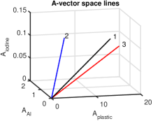
Fig. 1: Three lines in A-vector space used in the Monte Carlo simulation. Each line is the A-vectors of different thicknesses of a material with a specific $\mathbf{a}$ vector of coefficients in its attenuation coefficient expansion.

The test object attenuates the x-ray beam before it is incident on the detector so the rate of photon arrivals on the detector and therefore the pileup parameter, $\eta$, decreases as the object thickness increases along the lines in A-vector space.

II-H Compute CRLB for test object

A 120 kilovolt x-ray tube spectrum was computed using the TASMIP algorithm of Boone and Seibert[3]. The number of photons incident on the object for each detector element or pixel was set to $10^{6}$. The measurement time was assumed to be 10 milliseconds so the rate of photons incident on the detector with no object in the beam was $10^{8}$ photons per second. With detector deadtimes of 10 and 1 nanoseconds the zero object thickness pileup parameter, $\eta_{0}$, had values of 1 or 0.1.

The attenuation coefficients of the calibration phantom materials described in Sec. II-G were used as the basis functions of energy in Eq. 1. With this choice, the A-vectors were the thicknesses of each of the materials in the calibration phantom[14]. The attenuation coefficients of the materials were computed as the fraction by weight of each element in the chemical formula multiplied by the attenuation coefficient of that element. The elements’ attenuation coefficients were computed by piece-wise continuous Hermite polynomial interpolation of the standard Hubbell-Seltzer tables[4].

For a single A-vector on one of the lines in Fig. 1, the TASMIP x-ray tube spectrum and the basis material attenuation coefficients were used with Eq. 10 to compute the spectrum and the expected value of the total number of transmitted photons incident on the detector sensor during the measurement time. The sensor was assumed to be perfectly absorbing so the charge signal of each photon was proportional to the photon energy. Pulse height analysis was performed for the total energy of the photons incident on the sensor during the measurement time. As described in Sec. II-F, the PHA energy response functions were computed with an algorithm that maximized the SNR with no pileup and were assumed to be perfect rectangles. The CRLB was computed for three and four bin PHA.

The CRLB was computed numerically by approximating the derivatives in Eq. 7 from the first central difference. For example, to compute $\mathbf{\Delta L}$ we first compute the spectra through the object with attenuation $\mathbf{A}$ and then with $\mathbf{A+}\Delta\mathbf{A}$. The transmitted spectra are not affected by pileup since they occur before the measurement. These transmitted spectra are then used to compute the expected values of the measurements with pileup using the formulas in Sec. II-D.

II-I $\mathbf{M}$ condition number for test object

As discussed in Sec. II-E, we would expect the estimator noise variance to be large if the $\mathbf{M}$ matrix is ill-conditioned, that is, it has a large condition number. This was verified by simultaneously plotting the normalized $A_{1}$ variance and the $\mathbf{M}$ condition number along the three lines in A-vector space.

II-J $\mathbf{M}$ condition in 3D A-vector space

The CRLB and condition numbers showed sharp peaks in plots along the lines in A-vector space. To better characterize the behavior, the $\mathbf{M}$ matrix condition number was computed in three dimensional A-vector space. This was done by computing the $\mathbf{L}$ values with pileup on a 3D grid of points. The $\mathbf{M}$ matrices at each of the points were computed using the Matlab $gradient$ function, which approximates the gradient using the first central difference of the $\mathbf{L}$ vector data on the neighboring points. The condition number of the $\mathbf{M}$ at each point was then computed with the Matlab $cond$ function.

Two dimension data of the condition numbers in the $\left(A_{1},A_{2}\right)$ planes were extracted for each of the $A_{3}$ values. The local maxima in the 2D condition number data were found using the Matlab $imregionalmax$ function and their three dimension coordinates were saved. A three dimension plot of the positions of the peak values in the three dimension A-vector space was then created.

The pileup parameters $\eta$ on the A-vector space plane of peak condition numbers were computed.

II-K PHA data for large pileup case

To gain some insight into the cause of the non-invertibility, the relationship between the peaks in condition number and the count data in each of the PHA bins were computed as a function of object thickness by plotting the expected bin count values along the A-vector line for material 3 (see Fig. 1) in separate graphs.

III RESULTS

III-A CRLB for three and four bin PHA

Figures 3 and 3 show the CRLB noise variance as a function of position along the three lines in A-vector space in Fig. 1. In both figures, the zero object thickness pileup parameter, $\eta_{0}$, is 1 count per dead time, a relatively large value. Fig. 2 is for four bin PHA and Fig. 3 is for three bin.

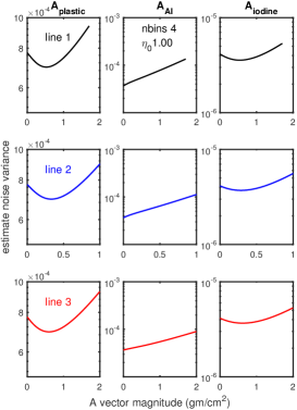
Fig. 2: Four bin PHA CRLB noise variance as a function of object thickness along the three lines in A-vector space in Fig. 1. There was a large, zero thickness pileup parameter, $\eta_{0}=1$.

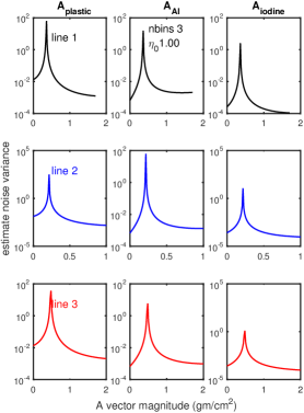
Fig. 3: Three bin PHA CRLB noise variance with $\eta_{0}=1$ as a function of object thickness. Note the peaks. They have variance values more than $10^{5}$ times larger than the 4-bin PHA variance in Fig. 2 for comparable thickness. A logarithmic y-axis scale is used.

Fig. 4 shows the estimates’ CRLB variance for three bin PHA with a relatively small zero thickness pileup parameter, $\eta_{0}=0.1$.

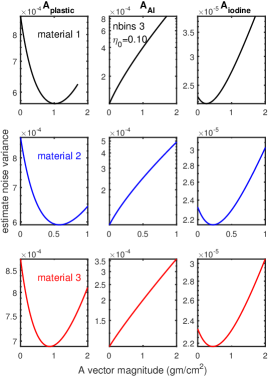
Fig. 4: Three bin PHA CRLB noise variance with low pileup, $\eta_{0}=0.1$. Compare with the high pileup case in Fig. 3. Notice that with low pileup there are no peaks in the variance. [5].

III-B M condition number and CRLB variance peaks

Fig. 5 shows plots of the $\mathbf{M}$ matrix condition number and the CRLB as a function of position on line 1. Note that the peaks in variance coincide with a large condition number i.e. ill-conditioned matrix.

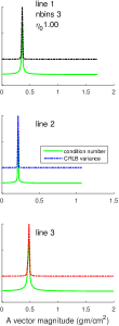
Fig. 5: CRLB variance peak coincides with M condition number peak. Plotted is the $A_{1}$ variance and the $\mathbf{M}$ condition number as a function of object thickness. For visualization, the values are normalized by dividing by the maximum and offset by subtracting 0.5 from the normalized condition numbers. The y-axis scale is linear.

III-C Three dimension plot of A-vectors of M condition number peaks

Fig. 6 shows the $\mathbf{M}$ matrix condition numbers on three planes in A-vector space displayed as gray scale images. The images show the $(A_{1},A_{2})$ planes for $A_{3}$ values of .02, .04, and .06 $g/cm^{2}$.

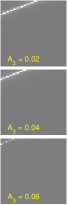
Fig. 6: Gray scale images of M matrix condition numbers on three planes in A-space. The images show the $(A_{1},A_{2})$ planes for $A_{3}$ values of .02, .04, and .06 $g/cm^{2}$.

Fig. 7 shows a 3D plot of the A-vectors of the peaks detected in the M matrix condition numbers images shown in Fig. 6. There are two views of the best fit plane. The side view in the bottom panel shows that the peaks are very close to the plane.

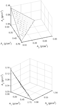
Fig. 7: Three dimension plot of M condition number peaks. The peaks are the black dots and the gray triangle is the best fit plane. Two views of the plane are shown. The top panel shows the peaks and the plane in a front view. The bottom panel is an edge-on view illustrating that the peaks are very close to the best fit plane.

Fig. shows the histogram of the pileup parameter $\eta$ on the plane of the peak variance in Fig. 7.

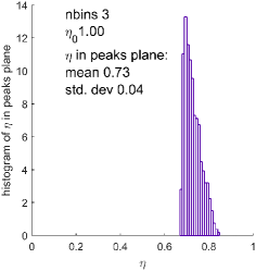
Fig. 8: Histogram of the pileup parameter $\eta$ on the plane of the peak variance in Fig. 7.

III-D PHA bin counts and estimator variance vs. object thickness

Fig. 9 shows the $\mathbf{L}$ vector components and the $A_{3}$ estimate variance as a function of the object thickness for line 3 in Fig. 1.

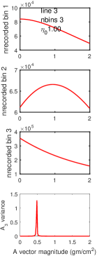
Fig. 9: The recorded photon counts for each PHA bin and the estimator variance as a function of the object thickness for line 3 in Fig. 1. The number of PHA bins is 3 and the zero thickness pileup parameter, $\eta_{0}=1$. The y-axis scale is linear.

IV DISCUSSION

Fig. 3 shows that with large pileup the three bin PHA data the CRLB variance exhibits a sharp peak that does not occur with the four bin PHA data results in Fig. 2. The peak is approximately $10^{5}$ times larger than four bin PHA variance at comparable object thickness. It is due to large pileup since the variance with three bin PHA data but with a small pileup parameter in Fig. 4 does not exhibit the peak.

Fig. 5 shows that the peak in variance coincides with a peak in the condition number of the $\mathbf{M}$ matrix. The reason for this is clear from the constant covariance approximation to the Fisher matrix in Eq. 7, $\mathbf{\left(M^{T}C_{L}^{-1}M\right)^{-1}}$. If $\mathbf{M}$ is ill-conditioned then the CRLB variance, which is its inverse, will be large.

Fig. 4 shows that, even though there are no peaks in variance with low pileup, the variance first decreases and then goes through a minimum as the object thickness increases. This is particularly evident in the $A_{plastic}$ component. This is contrary to the behavior with zero pileup where the variance increases monotonically with object thickness. With pileup, the pileup parameter $\eta$ decreases as object thickness increases because the rate of photon arrivals on the detector decreases. The decrease in pileup parameter causes the condition number of the $\mathbf{M}$ matrix to improve so even though the photon counts are decreasing the condition number improvement compensates and the A-vector variance decreases for small object thicknesses. As the object thickness increases above the initial range, the condition number does not decrease rapidly enough to compensate for the lower photon count and the noise variance increases.

The figures in Sec. III-C show that the $\mathbf{M}$ condition number peaks occur on a plane in 3D A-vector space. This implies that the inverse $\mathbf{L(A)}$ transformation becomes ill-conditioned for a specific attenuation. The histogram of the pileup parameter $\eta$ values on the plane in Fig. 8 shows that the values are approximately the same, $0.73\pm 0.04.$

The PHA bin count data for the three bin PHA, high pileup case in Fig. 9 show that the second bin data are not invertible since the curve has a zero derivative with respect to the A-vector magnitude plotted on the x-axis. The shape of the bin counts curve is due to the fact that, as the object thickness increases, the count rate and therefore the amount of pileup decreases rapidly. With less pileup there are fewer cases where the recorded energy is due to two or more photons. This tends to decrease the relative number of counts in the third high energy bin and to increase the relative number of counts in the first and second lower energy bins.

Notice however that the peak in variance and therefore $\mathbf{M}$ condition number, shown in the bottom panel of Fig. 9 does not occur at the zero derivative A-vector magnitude value but somewhat below that value.

High pileup severely distorts the recorded data and reduces its information content compared with the non-pileup case. The other defects of photon counting detectors noted in the Introduction also reduce the information content and it is reasonable that they may also lead to increased estimator noise variance. Therefore, designers of systems using these detectors should study the statistical properties of their data and conduct studies of the implication for the stability of the estimator output.

V CONCLUSION

Photon counting data with pileup can lead to sharply increased noise variance in the estimates of the line integrals of the basis set coefficients in the Alvarez-Macovski method. The increased noise occurs with high pileup three bin data but does not occur with four bin data or either three or four bin PHA data with low pileup. The peaks in noise variance occur for specific object attenuation. State of the art detectors have pileup as well as other defects so they may also exhibit the spikes in noise variance found in this study.

References

- [1] R. E. Alvarez and A. Macovski, “Energy-selective reconstructions in X-ray computerized tomography,” Phys. Med. Biol. 21, 733–44, (1976). [Online]. Available: http://dx.doi.org/10.1088/0031-9155/21/5/002
- [2] G. F. Knoll, Radiation Detection and Measurement, 3rd ed., Hoboken, N.J.: Wiley, 2000.
- [3] J. M. Boone and J. A. Seibert, “An accurate method for computer-generating tungsten anode x-ray spectra from 30 to 140 kV,” Med. Phys. 24, 1661–70, (1997). [Online]. Available: http://dx.doi.org/10.1118/1.597953
- [4] J. H. Hubbell, “Review of photon interaction cross section data in the medical and biological context,” Phys. Med. Biol. 44, R1–R22, (1999). [Online]. Available: http://dx.doi.org/10.1088/0031-9155/44/1/001
- [5] R. E. Alvarez, “Signal to noise ratio of energy selective x-ray photon counting systems with pileup,” Med. Phys. 41, no. 11, 111909, (2014). [Online]. Available: http://dx.doi.org/10.1118/1.4898102
- [6] S. M. Kay, Fundamentals of Statistical Signal Processing, Volume I: Estimation Theory , Upper Saddle River, NJ: Prentice Hall PTR, 1993, Ch. 3.
- [7] R. E. Alvarez, “Dimensionality and noise in energy selective x-ray imaging,” Med. Phys. 40, no. 11, 111909, (2013). [Online]. Available: http://dx.doi.org/10.1118/1.4824057
- [8] S. M. Kay, Fundamentals of Statistical Signal Processing, Volume I: Estimation Theory , Upper Saddle River, NJ: Prentice Hall PTR, 1993, Sec. 4.5.
- [9] K. Taguchi, M. Zhang, E. C. Frey, X. Wang, J. S. Iwanczyk, E. Nygard, N. E. Hartsough, B. M. W. Tsui, and W. C. Barber, “Modeling the performance of a photon counting x-ray detector for CT: energy response and pulse pileup effects,” Med. Phys. 38, 1089–1102, (2011). [Online]. Available: http://dx.doi.org/10.1118/1.3539602
- [10] D. F. Yu and J. A. Fessler, “Mean and variance of single photon counting with deadtime,” Phys. Med. Biol. 45, 2043–2056, (2000). [Online]. Available: http://dx.doi.org/10.1088/0031-9155/45/7/324
- [11] A. S. Wang, D. Harrison, V. Lobastov, and J. E. Tkaczyk, “Pulse pileup statistics for energy discriminating photon counting x-ray detectors,” Med. Phys. 38, 4265–4275, (2011). [Online]. Available: http://dx.doi.org/10.1118/1.3592932
- [12] Papoulis, Athanasios, Probability, Random Variables, and Stochastic Processes, McGraw-Hill, 1965.
- [13] L. N. Trefethen and D. Bau, Numerical Linear Algebra, Philadelphia: SIAM, 1997.
- [14] R. E. Alvarez and E. J. Seppi, “A comparison of noise and dose in conventional and energy selective computed tomography,” IEEE Trans. Nucl. Sci. NS-26, 2853–2856, (1979). [Online]. Available: http://www.dx.doi.org/10.1109/TNS.1979.4330549