A new computational method for a model of C. elegans biomechanics: Insights into elasticity and locomotion performance

Abstract.

An organism’s ability to move freely is a fundamental behaviour in the animal kingdom. To understand animal locomotion requires a characterisation of the material properties, as well as the biomechanics and physiology. We present a biomechanical model of C. elegans locomotion together with a novel finite element method. We formulate our model as a nonlinear initial-boundary value problem which allows the study of the dynamics of arbitrary body shapes, undulation gaits and the link between the animal’s material properties and its performance across a range of environments. Our model replicates behaviours across a wide range of environments. It makes strong predictions on the viable range of the worm’s Young’s modulus and suggests that animals can control speed via the known mechanism of gait modulation that is observed across different media.

1. Introduction

1.1. Background

Active motility and animal locomotion are fundamental for the survival of life forms across all scales. At the microscale, cells and microorganisms most commonly occupy fluid habitats often near surfaces. To orient themselves and navigate in their environments such microorganisms employ active swimming. In this low Reynolds number regime (Reynolds number $(\mathrm{Re})$ less than one), where viscous forces dominate over inertial forces, the scallop theorem (Purcell, 1977) prohibits self-propelled locomotion for time-reversal symmetric sequences of body postures (Taylor, 1952). It is therefore no accident that at this scale, locomotion most commonly relies on undulations, or the propagation of waves along the body or parts thereof, that break time-reversal symmetry (Cohen and Boyle, 2010).

Of particular interest in the study of undulatory locomotion and its neural basis is the roundworm (nematode) Caenorbabditis elegans. The animal’s invariant anatomy (959 nongonadal cells in the adult hermaphrodite of which exactly 302 are neurons), fully annotated cell lineage, genome and nervous system and its well characterised behaviours make it a leading model organism in neurobiology, developmental and molecular biology. With small size, an elegant periodic gait, and experimental tractability, this animal has also captured the interest of physicists, computer scientists and engineers, as a model system for active swimming, neuromechanics and biorobotics. While in the wild, C. elegans grows mostly in rotten vegetation, it is grown extensively in laboratories, where it is cultured on the surface of agar gels. With a length of $1\,\mathrm{mm}$ and up to $2\,\mathrm{Hz}$ undulation frequency, the worm can have a $\mathrm{Re}\approx 1$ in water based buffer solutions - approaching the upper bounds for a low $\mathrm{Re}$ treatment (Montenegro-Johnson et al., 2016). On agar, as well as in liquid, C. elegans move by propagating undulatory waves from head to tail to generate forward thrust (Gray and Lissmann, 1964; Croll, 1970; Pierce-Shimomura et al., 2008; Berri et al., 2009; Fang-Yen et al., 2010; Lebois et al., 2012). Body wall muscles, lining the dorsal and ventral sides of the body generate bending.

Close inspection of C. elegans crawling on the surface of an agar gel reveals a thin film of liquid on the surface and surrounding the animals. As the animal moves, surface tension presses it strongly against the gel surface (Wallace, 1968). To move, the animal carves a groove in the gel along its path, and in so doing, it leaves approximately periodic tracks in its wake. As the worm moves forwards, it overcomes the gel’s yield stress with its head, allowing the rest of the body to follow more easily. In contrast, motion normal to the body surface is strongly resisted. For a sufficiently stiff gel, the net result is functionally quite similar to locomotion in a solid channel (Fang-Yen et al., 2010; Berri et al., 2009). In contrast, in a Newtonian environment, such as buffer solution, normal and tangential forces are of comparable magnitude. The modulation of locomotory gait as a function of the properties of the fluid environment has been the focus of extensive work (Berri et al., 2009; Fang-Yen et al., 2010; Sznitman et al., 2010a; Sauvage et al., 2011; Cohen and Sanders, 2014), highlighting the importance of biomechanical models, as well as neurological and fluid models, of this important system (Niebur and Erdös, 1991; Boyle et al., 2012; Sznitman et al., 2010a; Fang-Yen et al., 2010; Cohen and Sanders, 2014; Szigeti et al., 2014; Palyanov et al., 2016; Montenegro-Johnson et al., 2016).

1.2. Model

In this work we present a continuum model of C. elegans biomechanics and derive a new numerical method that allows for simulations of arbitrary locomotion gaits. The model is based on previous formulations of bending in elastic beams given by Landau and Lifschitz (1975, Sec. 17-20) and Guo and Mahadevan (2008) which was originally applied to the locomotion of sandfish in granular media and has also been applied to the locomotion of C. elegans in Newtonian media, for example, see (Sznitman et al., 2010a; Fang-Yen et al., 2010).

In contrast to these previous approaches, we will use an inextensibility constraint derived from conservation of mass to close the model and thus allow the exploration of kinematic properties, including body postures predicted by the model as well as crawling speeds. Furthermore, we derive a new presentation of the model which yields a formulation better-suited to numerical computations to solve the full nonlinear system of equations.

1.3. Numerical method

We will solve the model using a novel parametric finite element method. In this approach the midline curve of the worm is approximated by a piecewise linear curve and the local length constraint is enforced using a piecewise constant line tension in a so-called mixed finite element method. A semi-implicit time stepping strategy is used which produces a linear system of equation to solve at each time step. Our approach builds on the method of Dziuk et al. (2002) for the elasticae equations which have a global length constraint instead of our local constraint. A key step in the method is to introduce a new variable for curvature which permits the use of piecewise linear finite elements. A semi-discrete error bound is provided by Deckelnick and Dziuk (2009). For models without the local length constraint, moving the nodes purely according to the model may result in very distorted mesh points which may lead to break down of the method. Barrett et al. (2010, 2011) introduce an artificial tangential motion which avoids this type of break down. A separate approach using a $C^{1}$-splines which capture the curvature directly in a conforming method for an inextensible elastic beam has been studied by Bartels (2013). Here, the local length constraint ensures that the mesh points do not become too distorted.We propose a different formulation of the constraint equation which leads to a more accurate and robust numerical scheme whilst also working with the simpler finite element spaces. A review of different finite element approaches to geometric partial differential equations is given by Deckelnick et al. (2005).

1.4. Outline

We will demonstrate the applicability of the method in simulations to investigate biomechanical properties of the worm, to investigate body shapes during rhythmic forward locomotion and to illustrate the capacity of the active body to generate non-undulatory body shapes, reminiscent of omega turns, which the worm uses to reorient Gray et al. (2005). Furthermore we will investigate limits of physical properties and movement envelope of the animal through different media which will show the evolutionary trade offs involved.

The rest of the manuscript proceeds as follows. In Section 2, we introduce the model of Guo and Mahadevan (2008) with our new closing assumptions. Our focus in this section is to provide sufficient detail to see where important biological details are included. This section includes details of a non-dimensionalisation which allows us to consider important parameter relationships. Section 3 presents the numerical method and also provides mathematical results to show the key properties of the numerical scheme. We conclude, in Section 4, with numerical results to show how the model and numerical scheme can be used to simulate important parameter regimes.

2. Model

We present the model in detail in order to demonstrate where important biological details are included which could be controlled in appropriate experimental assays. We aim to write the model in a way that is suitable for numerical computations so work with a parametrisation which is not necessarily an arc-length parametrisation.

In C. elegans and other nematodes, the body is well approximated by a tapered cylinder. A body cavity with high hydrostatic pressure ensures that the volume of the worm is approximately conserved. A viscoelastic cuticle encapsulates the animal. 95 body wall muscles line the body in four quadrants. The muscles are driven by motor neurons in the head and along the body. Muscles are attached to the cuticle, such that their contractions induce bending. The neuromuscular connectivity pattern along the body restricts muscle contractions to the dorso-ventral plane, limiting experimental studies and models to date to two dimensions. To move, the animal lies on its left or right side, propagating body waves in the dorso-ventral plane, opposite the direction of motion. As we focus on nematodes, we therefore assume that the worm is positioned on its side (Hart, 2006).

For a sufficiently slender worm, a model of a viscoelastic beam captures the key properties of the biomechanics and kinematics of the locomotion embedding in fluid which vary across a wide range of viscosities (Fang-Yen et al., 2010) and effective viscoelasticities (Berri et al., 2009; Boyle et al., 2012). More recent models have instead modelled a cylindrical shell (Sznitman et al., 2010a) highlighting the finite aspect ratio of the animal (length to diameter ratio $\approx 12$) with attached muscles promoting the direct actuation of the thin cuticle. Here, we model the cuticle by a thin viscoelastic shell, and derive the effective force equations on the midline of the body. Note that throughout, our reference to the elasticity of the cuticle is used only loosely. Strictly speaking, our elasticity term couples contributions for the cuticle and the interior of the worm. Further work is needed to decouple these contributions (Gilpin et al., 2015).

We assume that the geometry of the worm at time can be described through a parametrisation in cylindrical geometry:

$$\mathcal{W}(t):=\{\boldsymbol{x}(u,t)+B(0,R(u)):u\in[0,1]\}\subset\mathbb{R}^{3},$$

where $\boldsymbol{x}(\cdot,t)\colon[0,1]\to\mathbb{R}^{2}\times\{0\}$ is a smooth parametrisation of the midline $\mathcal{C}(t)$ of $\mathcal{W}(t)$, $R(u)$ is the radius of the worm at $\boldsymbol{x}(u,t)$ and $B(0,R(u))$ is a disk radius $R(u)$ in the normal plane to $\mathcal{C}(t)$ at $\boldsymbol{x}(u,t)$. We assume that the radius of the worm is fixed in time but may vary along the parametrised length of the worm $u$ and that the worm has a constant density $\varrho$.

We will choose the dimensionless variable $u$ a material coordinate which corresponds monotonically to a body coordinate. Tracking a point $\boldsymbol{x}(u,t)$ in time corresponds to following a fixed marker within the worm. Thus $u$ is an anatomically and physiologically relevant physical variable. Here, we take $\boldsymbol{x}(0,t)$ and $\boldsymbol{x}(1,t)$ to denote the head and tail of the animal, respectively. The choice of a potentially non-arclength parametrisation allows us to naturally impose the forces resulting from internal pressure whilst also giving greater flexibility when working with this geometry in a computational setting. Furthermore, the choice of parametrisation provides a much more general framework for following material coordinates in a wider variety of soft-bodied locomotion including when considering organisms which vary in length (Paoletti and Mahadevan, 2014).

2.1. Geometry

We denote by $\boldsymbol{\tau}$ the unit tangent vector, by $\boldsymbol{\nu}$ the unit normal vector in the plane $\mathbb{R}^{2}\times\{0\}$ and by $\boldsymbol{\kappa}(u,t)$ the vector curvature of $\mathcal{C}(t)$. We can define these essential geometric quantities using the parametrisation of the midline $\boldsymbol{x}$:

(1a) $$\boldsymbol{\tau}(u,t)=\boldsymbol{\tau}(\boldsymbol{x}(u,t),t) =\frac{\boldsymbol{x}_{u}(u,t)}{\left|\boldsymbol{x}_{u}(u,t)\right|},\quad\boldsymbol{\nu}(u,t)=\boldsymbol{\nu}(\boldsymbol{x}(u,t),t)=\left(\frac{\boldsymbol{x}_{u}(u,t)}{\left|\boldsymbol{x}_{u}(u,t)\right|}\right)^{\perp}$$

(1b) $$\boldsymbol{\kappa}(u,t)=\boldsymbol{\kappa}(\boldsymbol{x}(u,t),t) =\frac{1}{\left|\boldsymbol{x}_{u}(u,t)\right|}\frac{\partial}{\partial u}\boldsymbol{\tau}(u,t)=\frac{1}{\left|\boldsymbol{x}_{u}(u,t)\right|}\frac{\partial}{\partial u}\left(\frac{\boldsymbol{x}_{u}(u,t)}{\left|\boldsymbol{x}_{u}(u,t)\right|}\right),$$

where we choose the orientation $(\xi_{1},\xi_{2},0)^{\perp}:=(-\xi_{2},\xi_{1},0)$ for the normal vector. It can be shown that the vector curvature points in the normal direction so that if $\boldsymbol{\kappa}\neq 0$, we can decompose $\boldsymbol{\kappa}=\kappa\boldsymbol{\nu}$ to determine the (signed) scalar curvature $\kappa$. The scalar curvature sign depends on the local convexity/concavity of the worm with respect to the choice of orientation of $\boldsymbol{\nu}$. The relevant quantities are shown in Figure 1.

Remark 1.

In previous work on C. elegans locomotion the Frenet frame has been used to define the unit normal vector field as $\boldsymbol{\nu}:=\boldsymbol{\kappa}/\left|\boldsymbol{\kappa}\right|$ (Stephens et al., 2008). The above definition remains valid when $\boldsymbol{\kappa}=0$ and chooses a consistent normal direction.

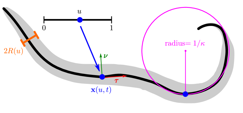
Figure 1. A sample worm posture marked up with our geometric description. The worm outline $\mathcal{W}$ in the plane is shown in grey and the midline $\mathcal{C}$ is shown in black which is parametrised by $\boldsymbol{x}$ with width $2R$. The tangent vector $\boldsymbol{\tau}$ (red) and normal vector $\boldsymbol{\nu}$ (green) are shown. The pink osculating circle shows the radius of curvature which is the inverse of the absolute value of the scalar curvature and is equal to $\pm\left|\kappa\right|$

.

Although we will write our model with respect to the parameter $u$, we will also make use of an arc-length parameter $s=s(u)$ defined by

$$s=s(u)=\int_{0}^{u}\left|\boldsymbol{x}_{u}\right|\,\mathrm{d}u.$$

In particular $\partial/\partial s=\left|\boldsymbol{x}_{u}\right|^{-1}\partial/\partial u$. The variable $s$ represents the physical length along the body.

2.2. Derivation of equations

Conservation laws

We start by considering conservation of mass and recall that we have assumed that the density of the worm, $\varrho$, is constant. Let $\Gamma(t)$ be a portion of the worm that follows the motion of $\mathcal{W}(t)$ then

$$\frac{d}{dt}\int_{\Gamma(t)}\varrho\,\mathrm{d}\Gamma=\varrho\frac{d}{dt}\int_{\Gamma(t)}\,\mathrm{d}\Gamma=0.$$

In particular for $\Gamma(t)=\{\boldsymbol{x}(u,t)+B(0,R(u)):u\in(u_{1},u_{2})\}$ for arbitrary $0\leq u_{1}<u_{2}\leq 1$, we see that since $R(u)$ is fixed in time and $\varrho$ is a constant that

$$\frac{d}{dt}\int_{\Gamma(t)}\varrho\,\mathrm{d}\Gamma=\varrho\frac{d}{dt}\int_{u_{1}}^{u_{2}}\pi R(u)^{2}\left|\boldsymbol{x}_{u}\right|\,\mathrm{d}u=\varrho\int_{u_{1}}^{u_{2}}\pi R(u)^{2}\boldsymbol{\tau}\cdot\boldsymbol{x}_{u,t}\,\mathrm{d}u=0.$$

Since this equation holds for all $0\leq u_{1}<u_{2}\leq 1$ and $\varrho,R(u)>0$, we have that

(2) $$\frac{d}{dt}\left|\boldsymbol{x}_{u}\right|=\boldsymbol{\tau}\cdot\boldsymbol{x}_{u,t}=0.$$

We may integrate (2) forwards in time to see that $\left|\boldsymbol{x}_{u}\right|$ is invariant in time. This implies that the length of the midline curve is fixed. If the initial condition is a proportional to an arc-length parametrisation, then the parametrisation is proportional to an arc-length parametrisation at all times. We will use this in Section 3 to impose a parametrisation which is approximately proportional to arc-length. We will not directly substitute the initial values of $\left|\boldsymbol{x}_{u}\right|$ into our geometry since we wish to be able to track the errors in our approximation.

We denote by $\boldsymbol{F}$ the internal force resultant, $\boldsymbol{M}=(0,0,M)$ the internal moment resultant, and by $\boldsymbol{K}$ the external force per unit length at each cross section. Neglecting inertia (Fang-Yen et al., 2010; Berri et al., 2009) conservation of linear and angular momentum give the relations that (Landau and Lifschitz, 1975, Eq. 19.2,19.3)

(3) $$\boldsymbol{F}_{s}+\boldsymbol{K}=0,\qquad\boldsymbol{M}_{s}+\boldsymbol{\tau}\times\boldsymbol{F}=0,$$

We decompose $\boldsymbol{F}=p\boldsymbol{\tau}+N\boldsymbol{\nu}$ into transverse shear force $N$ and tangential force (line tension) $p$ and the moment $M=M^{p}+M^{a}$ into passive $M^{p}$ and active $M^{a}$ components.

Interaction with the environment

We model the worm’s interaction with the its surrounding fluid using slender body theory. In a low Reynolds number, Newtonian environment where the fluid boundaries effect are negligible, the environmental forces can be described using a Stokes system. The fluid system can be solved using the Stokeslet which reduces to normal $(K_{\boldsymbol{\nu}})$ and tangential $(K_{\boldsymbol{\tau}})$ drag coefficients. This simplified formulation is also known as resistive force theory (Gray and Hancock, 1955). A key property of this system is the ratio of drag coefficients, $K:=K_{\boldsymbol{\nu}}/K_{\boldsymbol{\tau}}$.

Lighthill (1976) derived that, in water-like buffer solution, $\boldsymbol{K}$ should be given by

(4) $$\boldsymbol{K}=-K_{\boldsymbol{\nu}}(\boldsymbol{x}_{t}\cdot\boldsymbol{\nu})\boldsymbol{\nu}-K_{\boldsymbol{\tau}}(\boldsymbol{x}_{t}\cdot\boldsymbol{\tau})\boldsymbol{\tau},\quad K_{\boldsymbol{\nu}}=\frac{2\pi\mu}{\log(2\alpha/R)},K_{\boldsymbol{\tau}}=\frac{4\pi\mu}{\log(2\alpha/R)+0.5},$$

where $\mu$ is the dynamic viscosity of the fluid ($\approx 1\,\,\mathrm{mPa}\,\,\mathrm{s}$ for water), and $R$ is the radius of the body. The factor $\alpha$ depends on the precise waveform of undulations. For sinusoidal and sufficiently small amplitude undulations with $\lambda=1.5\,\mathrm{mm}$, Lighthill (1976) showed that $\alpha\approx 0.09\lambda$. Note that the ratio $K$ is purely geometric entity in Newtonian fluids (independent of viscosity).

Remark 2.

Note that our definitions of $K_{\boldsymbol{\nu}}$ and $K_{\boldsymbol{\tau}}$ differ from Boyle et al. (2012) by a factor of $L$ since $\boldsymbol{K}$ is force per unit length.

Following Berri et al. (2009), we will assume that the resistive force description is permissible in the case of select viscoelastic (non-Newtonian) fluids. As in this regime (4) no longer applies, we will use experimentally derived coefficients.

Recent works by Schulman et al. (2014) have used an extension of this theory to include the so-called wall effects from small scale swimmers moving near the boundary of the surrounding fluid. Rabets et al. (2014) have also considered a nonlinear correction to this linear theory to account for nonlinear force-velocity relationships induced by viscoelastic effects in the surrounding fluid. In this work, we assume that we remain in the linear regime as predicted by slender body theory and validated by (Berri et al., 2009) and limit our consideration to locomotion far from boundaries, so that wall effects are negligible.

Passive moment

The passive moment is given by considering the stress over the disc $B(0,R(u))$ centered at each point along the midline:

$$M^{p}(u,t)=\int_{B(0,R(u))}\rho\sigma\,\mathrm{d}A,$$

where $\rho$ is the distance to the centre of $B(0,R(u))$, $\sigma$ is the stress, $\mathrm{d}A$ is the area element in $B(0,R(u))$. The passive properties of the worm are given by assuming a linear Voigt model for the visco-elastic cuticle (Fung, 1993; Linden, 1974) so that

$$\sigma=E\epsilon+\eta\epsilon_{t},$$

where $\epsilon$ is the strain, $E$ is the Young’s modulus of the cuticle, and $\eta$ is the viscosity of the cuticle. Since the mechanical stress arises in the cuticle, we have that $\sigma$ is zero away from the thin cuticle. This continuum model of the viscoelastic properties of the cuticle more naturally captures the forces given by the parallel springs and dampers in the articulated model of Boyle et al. (2012).

Assuming that we only allow deformations along the body (no rotational or radial deformations), we can compute from our cylindrical parametrisation that (Landau and Lifschitz, 1975, Sec. 17)

$$\epsilon(u,\rho,t)=\rho\kappa(u,t).$$

Here, we use a reference configuration of a straight line of length $L$ and applied the conservation of mass. We infer that the passive moment is given by

(5) $$M^{p}=EI_{2}\kappa+\eta I_{2}\kappa_{t}.$$

Here $I_{2}$ is the second moment of area of the cuticle given by

$$I_{2}(u)=\int_{B(0,R(u))}\rho^{2}\,\mathrm{d}A=\frac{\pi}{2}\left[(R+r_{\mathrm{cuticle}}/2)^{4}-(R-r_{\mathrm{cuticle}}/2)^{4}\right],$$

where $r_{\mathrm{cuticle}}$ is the thickness of the cuticle.

Remark 3.

Recent experimental evidence has shown that the properties of the cuticle may not follow such a simple relationship. Backholm et al. (2015b) propose that a power-law fluid model which was shown to be in good agreement with experimental results. For this preliminary work, we pursue this simple model and leave more complicated constitutive relations to future work.

Internal pressure

We have modelled our worm in an idealised situation by strictly enforcing a strict inextensibility constraint (2). In this situation, instead of using a constitutive relation for the resulting line tension of $\mathcal{C}$, which we denote by $p\boldsymbol{\tau}$, we treat the magnitude of the line tension as a dynamic variable and must be determined from the other equations in our model (Coomer et al., 2001). In this way, we see that $p\boldsymbol{\tau}$ may be considered as the effective force resulting from internal pressure, or mathematically a Lagrange multiplier, which enforces mass conservation. We note that such a treatment of pressure is conventional in fluid mechanics (Batchelor, 2000).

Model and boundary conditions

We consider the above equations over a fixed time interval $[0,T]$. We assume that a smooth initial condition $\boldsymbol{x}_{0}$ is given which satisfies $\left|\boldsymbol{x}_{0,u}\right|\geq\gamma>0$ for some positive constant $\gamma$. Combining the conservation laws (2) and (3) with the external force (4) and passive moment (5) leads to the following system of equations which we now write with respect to the parameter $u$:

Given an initial condition $\boldsymbol{x}_{0}$ and an active moment $M^{a}$, find $\boldsymbol{x}\colon[0,1]\times(0,T)\to\mathbb{R}^{2}\times\{0\}$ and $p\colon[0,1]\times(0,T)\to\mathbb{R}$ such that

(6) $$K_{\boldsymbol{\nu}}(\boldsymbol{x}_{t}\cdot\boldsymbol{\nu})\boldsymbol{\nu}+K_{\boldsymbol{\tau}}(\boldsymbol{x}_{t}\cdot\boldsymbol{\tau})\boldsymbol{\tau}-\frac{1}{\left|\boldsymbol{x}_{u}\right|}(p\boldsymbol{\tau})_{u}$$

$$+\frac{1}{\left|\boldsymbol{x}_{u}\right|}\left(\frac{EI_{2}}{\left|\boldsymbol{x}_{u}\right|}\kappa_{u}\boldsymbol{\nu}+\frac{\eta I_{2}}{\left|\boldsymbol{x}_{u}\right|}\kappa_{tu}\boldsymbol{\nu}+\frac{1}{\left|\boldsymbol{x}_{u}\right|}M^{a}_{u}\boldsymbol{\nu}\right)_{u} =0$$

$$\boldsymbol{\tau}\cdot\boldsymbol{x}_{tu} =0$$

$$\boldsymbol{x}(\cdot,0) =\boldsymbol{x}_{0}.$$

We close the system by imposing zero moment and zero force at the two boundary ends:

$$-p\boldsymbol{\tau}+\left(\frac{EI_{2}}{\left|\boldsymbol{x}_{u}\right|}\kappa_{u}+\frac{\eta I_{2}}{\left|\boldsymbol{x}_{u}\right|}\kappa_{tu}+\frac{1}{\left|\boldsymbol{x}_{u}\right|}M^{a}_{u}\right)\boldsymbol{\nu} =0 \mbox{ for }u=0,1,$$

$$EI_{2}\kappa+\eta I_{2}\kappa_{t}+M^{a} =0 \mbox{ for }u=0,1.$$

Active moment

We conclude this section with a brief discussion of the active moment. In previous studies of worm locomotion, authors have developed integrated models which close the loop by including a nervous system which takes input from the body shape and outputs muscle deformations which lead to an active moment. In C. elegans, body wall muscles line the cuticle (or body wall). We assume a smooth and uniform muscle configuration along the body such that the muscle midline parametrisation is identical to that of the worm’s cuticle $u$. In Boyle et al. (2012), the muscle and cuticle lengths were considered as one. In contrast, here, we allow muscle lengths to drive the bending dynamics of the passive cuticle.

Consider a fixed muscle configuration so that $M^{a}(u,t)=M^{a}(u)$ and suppose the body of the worm is allowed to relax to stationary posture. As time tends to infinity, we see that

$$M^{a}=-EI_{2}\kappa.$$

In other words, for a stationary worm, the active moment is proportional to the resulting curvature. Indeed, we can take the same scaling and consider that $M^{a}$ is a preferred curvature in a similar fashion to the models of Helfrich (1973) for elastic lipid bilayers. We denote the preferred curvature arising from the muscle activation profile by $\beta$ and will use the relation $M^{a}=-EI_{2}\beta$.

Many previous experimental (Feng et al., 2004; Cronin et al., 2005; Karbowski et al., 2006; Ramot et al., 2008; Berri et al., 2009) and theoretic studies (Boyle et al., 2012; Butler et al., 2014; Backholm et al., 2015a) have characterised the muscle activation profile for forwards locomotion. The undulations of the animal are well described by a travelling wave for which the undulation amplitude, angular frequency and wavelength all vary with the resistivity of the fluid environment (Berri et al., 2009). For simplicity (neglecting the variation of wavelength along the body), we take the preferred curvature $\beta$ to be given by a periodic travelling wave of the form:

(7) $$\beta(u,t)=\beta_{0}(u)\Psi\left(\frac{2\pi Lu}{\lambda}-2\pi t\omega\right),$$

where $\Psi$ is a $2\pi$-periodic function, $\beta_{0}$ is the amplitude, $\lambda$ is the wavelength of undulations and $\omega$ is the angular frequency. Note that here, the driving force $\beta$ follows the material coordinate $u$ (corresponding to the physiological muscle locations).

2.3. Non-dimensionalisation and parameter choices

In this section, we introduce characteristic values for certain parameters in order to identify key relations within the system. In this way, we translated from important parameters for individual components of the model to important parameters of the system. All used parameters are given with references in Table 1.

The anatomy of the worm is very well characterised and highly consistent across individuals (Corsi, 2015). We take $L=1\,\mathrm{mm}$ and $R_{\mathrm{cuticle}}=0.5\,\mathrm{\mu m}$. The radius of the worm is typically given by $\bar{R}=40\,\mathrm{\mu m}$, but in fact varies along its length. We describe this using the function

$$R(u)=\bar{R}\frac{2\big{(}(\varepsilon/L+u)(\varepsilon/L+1-u)\big{)}^{\frac{1}{2}}}{{1+2\varepsilon/L}}$$

where $\varepsilon$ is a small distance chosen to regularise so that the worm always has strictly positive radius. The function is chosen to approximate the anatomical shape of the worm when the material coordinate $u$ is approximately proportional to arc-length (see below).

The material parameters of the worm are less well characterised with some estimates varying five order in magnitude. Of particular interest here is the choice of Young’s modulus $E$ for the cuticle of the worm, with estimates varying from $\approx 1\,\mathrm{kPa}$ (similar to that of sea anemonies) to $\approx 100\,\mathrm{MPa}$ roughly corresponding to the stiffness of rubber (Vogel, 1988; Vincent and Wegst, 2004). By comparison, the elasticity of elastin (a key constituent of vertebrate skin and connective tissue) is estimated at $\approx 1\,\mathrm{MPa}$. Insect cuticles alone, from different animals, developmental stages and conditions, cover a vast range of $E$ values from $\approx 10\,\mathrm{kPa}$ in some larvae to even to $\approx 10\,\mathrm{GPa}$.

The first approach to determining the elastic behaviour of the worm was by Park et al. (2007). The authors used a piezoresistive displacement clamp and saw a linear relationship between force and displacement and that the elasticity of the cuticle shell dominates the worm’s body stiffness. They estimate a value of $E$ to be $380\,\mathrm{MPa}$. However, the authors also note that the stiffness of the cuticle is likely to be different in the longitudinal and circumferential directions and likely that the longitudinal bending constant is lower. Another approach was given by Sznitman et al. (2010a) who fitted parameters in a simplified version of the model presented in this paper to high speed video recordings of freely moving worms. Based on an assumed ansatz for the muscle activation profile, they estimate that $E=3.77\pm 0.62\,\mathrm{kPa}$ and $\eta=-860.2\pm 99.4\,\mathrm{Pa}\,\mathrm{s}$ and that these values may vary with the environmental conditions (viscosity of the surrounding fluid) (Sznitman et al., 2010b). However, these results are sensitive to the choice of muscle activation ansatz and do not decouple passive and active muscle effects. A third approach was given by Fang-Yen et al. (2010) to augment the procedure of Sznitman et al. (2010a) by trapping the head of the worm in a micropipette with a second micropipette used to deflect the worm. The authors then studied the relaxation time of the worm’s shape. Using the simplified version of our model, they estimated that $E=13\,\mathrm{MPa}$ and $\eta<68\,\mathrm{kPa}\,\mathrm{s}$. More recently, Backholm et al. (2013) have use a similar micropipette deflection technique with an alternative model that estimates $E=1.3\pm 0.3\,\mathrm{MPa}$. Discounting, the extreme values due to different possible side effects of the methodologies used we will take values of $E=10\,\mathrm{MPa}$ and $\eta=50\,\mathrm{kPa}\,\mathrm{s}$ (except where otherwise stated).

We consider a range of different viscous and viscoelastic fluid environments. For Newtonian media, $K\approx 1.5$ and the viscosity values range experienced in common experimental conditions varies by more than 6 orders of magnitude (Fang-Yen et al., 2010). Parameter values for two special cases of the lower limiting case of buffer solution (denoted liquid) and viscosity yielding similar locomotion to that found on agar are given in Table 1. For non-Newtonian media, we limit ourselves to linear viscoelastic fluids, in which the undulations are well described by the ratio of drag coefficients $K_{\mathrm{liquid}}\leq K<100$ (Berri et al., 2009), but the corresponding values of effective drag coefficients are not well known (Boyle et al., 2012).

For liquid we can use the formulae given in (4) to determine the local drag coefficients experienced by the worm. Using the viscosity of liquid ($\mu\approx 1\,\mathrm{mPa}\,\mathrm{s}$) and typical dimensions of the worm’s locomotion ($q=0.09\lambda=1.35\cdot 10^{-4}\,\mathrm{m}$, $L=1\,\mathrm{mm}$) and typical radius $\bar{R}$ to give

$$K_{\boldsymbol{\nu},\mathrm{liquid}}=5.2\cdot 10^{-3}\,\mathrm{kg}\,\mathrm{m}^{-1}\,\mathrm{s}^{-1},\qquad K_{\boldsymbol{\tau},\mathrm{liquid}}=3.3\cdot 10^{-3}\,\mathrm{kg}\,\mathrm{m}^{-1}\,\mathrm{s}^{-1}.$$

For agar, Wallace (1969) estimated the tangential drag coefficients by measuring the force required to pull glass fibres of similar dimension to C. elegans across the surface of the gel. This method has been augmented by Niebur and Erdös (1991) and Berri et al. (2009) to give the coefficients we will use in this work. The process results in:

$$K_{\boldsymbol{\nu},\mathrm{agar}}=128\,\mathrm{kg}\,\mathrm{m}^{-1}\,\mathrm{s}^{-1},\qquad K_{\boldsymbol{\tau},\mathrm{agar}}=3.2\,\mathrm{kg}\,\mathrm{m}^{-1}\,\mathrm{s}^{-1}.$$

Parameter	Name	Typical value	Notes and references
$L$	Worm length	$1\,\mathrm{mm}$	Corsi (2015)
$\bar{R}$	Worm radius	$40\,\mathrm{\mu m}$	Corsi (2015)
$r_{\mathrm{cuticle}}$	Cuticle width	$0.5\,\mathrm{\mu m}$	Park et al. (2007);
			Sznitman et al. (2010a)
$E$	Young’s modulus	$10\,\mathrm{MPa}$	Park et al. (2007);
			Sznitman et al. (2010a);
			Fang-Yen et al. (2010);
			Backholm et al. (2013)
$\eta$	Cuticle viscosity	$50\,\mathrm{kPa}\,\mathrm{s}$	Sznitman et al. (2010a);
			Fang-Yen et al. (2010)
$(K_{\boldsymbol{\nu}},K_{\boldsymbol{\tau}})_{\mathrm{liquid}}$	Drag coefficients	$(5.2,3.3)\cdot 10^{-3}\,\mathrm{kg}\,\mathrm{m}^{-1}\,\mathrm{s}^{-1}$	Lighthill (1976);
	(buffer solution)		Boyle et al. (2012)
$(K_{\boldsymbol{\nu}},K_{\boldsymbol{\tau}})_{\mathrm{agar}}$	Drag coefficients (agar)	$(128,3.2)\,\mathrm{kg}\,\mathrm{m}^{-1}\,\mathrm{s}^{-1}$	Boyle et al. (2012)
$\beta_{0}$	Muscle wave amplitude (agar)	$8\,\mathrm{mm}^{-1}$	Boyle et al. (2012)
$(\omega,\lambda)_{\mathrm{liquid}}$	Muscle wave properties (7)	$(1.76\,\mathrm{s}^{-1},1.54\,\mathrm{mm})$	Fang-Yen et al. (2010)
	(buffer solution)
$(\omega,\lambda)_{\mathrm{agar}}$	Muscle wave properties (7)	$(0.30\,\mathrm{s}^{-1},0.65\,\mathrm{mm})$	Fang-Yen et al. (2010)
	(agar)

Table 1. List of used parameters with sources.

With typical values for each of the parameters fixed, we can now rescale the equations. We take a characteristic length scale $x_{c}$, characteristic time scale $t_{c}$ and characteristic line tension $p_{c}$ and introduce new non-dimensional variables by

$$\tilde{\boldsymbol{x}}=\boldsymbol{x}/x_{c},\qquad\tilde{t}=t/t_{c},\qquad\tilde{p}=p/p_{c},$$

Note that $u$ is already non-dimensional and these scalings induce a new scaled curvature $\tilde{\kappa}=\kappa x_{c}$ and final time $\tilde{T}=T/t_{c}$. Since $r_{\mathrm{cuticle}}\ll\bar{R}$, we see that

$$I_{2}\approx 2\pi R^{3}r_{\mathrm{cuticle}},$$

which we rescale as

$$\tilde{I}_{2}(u)=I_{2}/I_{c}=\frac{8\big{(}(\varepsilon/L+u)(\varepsilon/L+1-u)\big{)}^{3/2}}{(1+2\varepsilon/L)^{3}},\qquad\mbox{ where }I_{c}=2\pi\bar{R}^{3}r_{\mathrm{cuticle}}.$$

Note that $\tilde{I}_{2}(L/2)=1$. The values in Table 1 give that $I_{c}=2.0\cdot 10^{-19}\,\mathrm{m}^{4}$. We nondimensionalise the preferred curvature due the muscle forcing as:

$$\tilde{\beta}(u,t)=(\beta_{0}x_{c})\Psi\left(\frac{2\pi u}{\tilde{\lambda}}-2\pi\tilde{t}\tilde{\omega}\right),$$

where $\tilde{\lambda}=\lambda/L$ and $\tilde{\omega}=\omega t_{c}$.

For freely moving worms on agar, we choose:

$$x_{c}=L=1.0\,\mathrm{mm},\qquad t_{c}=1/\omega=3.3\,\mathrm{s},\qquad p_{c}=\frac{K_{\boldsymbol{\nu},\text{agar}}x_{c}^{2}}{t_{c}}=9.6\cdot 10^{-7}\,\mathrm{N}.$$

This results in:

$$K(\tilde{\boldsymbol{x}}_{\tilde{t}}\cdot\tilde{\boldsymbol{\nu}})\tilde{\boldsymbol{\nu}}+(\tilde{\boldsymbol{x}}_{\tilde{t}}\cdot\tilde{\boldsymbol{\tau}})\tilde{\boldsymbol{\tau}}-\frac{1}{\left|\tilde{\boldsymbol{x}}_{u}\right|}(\tilde{p}\tilde{\boldsymbol{\tau}})_{u}\qquad\qquad$$

$$+e\frac{1}{\left|\tilde{\boldsymbol{x}}_{u}\right|}\left(\frac{\tilde{I}_{2}}{\left|\tilde{\boldsymbol{x}}_{u}\right|}(\tilde{\kappa}-\tilde{\beta})_{u}\tilde{\boldsymbol{\nu}}\right)_{u}+\tilde{\eta}\frac{1}{\left|\tilde{\boldsymbol{x}}_{u}\right|}\left(\frac{\tilde{I}_{2}}{\left|\tilde{\boldsymbol{x}}_{u}\right|}\tilde{\kappa}_{\tilde{t}u}\tilde{\boldsymbol{\nu}}\right)_{u} =0$$

$$\left.-\tilde{p}\tilde{\boldsymbol{\tau}}+e\left(\frac{\tilde{I}_{2}}{\left|\tilde{\boldsymbol{x}}_{u}\right|}(\tilde{\kappa}-\tilde{\beta})_{u}\right)\tilde{\boldsymbol{\nu}}\right|_{u=0,1} =0$$

$$\left.e\tilde{I_{2}}(\tilde{\kappa}-\tilde{\beta})\right|_{u=0,1} =0$$

$$=0$$

$$\tilde{\boldsymbol{\tau}}\cdot\frac{1}{\left|\tilde{\boldsymbol{x}}_{u}\right|}\tilde{\boldsymbol{x}}_{\tilde{t}u} =0$$

$$\tilde{\boldsymbol{x}}(\cdot,0) =\tilde{\boldsymbol{x}}_{0},$$

where

$$K:=K_{\boldsymbol{\nu},\mathrm{agar}}/K_{\boldsymbol{\tau},\mathrm{agar}}=39,\qquad e:=\frac{EI_{c}t_{c}}{x_{c}^{4}K_{\boldsymbol{\tau},\mathrm{agar}}}=1.0$$

$$\qquad\mbox{ and }\qquad\tilde{\eta}:=\frac{\eta I_{c}}{x_{c}^{4}K_{\boldsymbol{\tau},\mathrm{agar}}}=1.6\cdot 10^{-3}\ll 1.$$

The results in agar are consistent with findings of Niebur and Erdös (1991); Fang-Yen et al. (2010) and Boyle et al. (2012) that internal viscosity of the worm is negligible for locomotion in sufficiently resistive environments. We remark, however, that by considering the worm’s locomotion in buffer solution we would recover $\tilde{\eta}\approx 1$ and so internal viscosity is important in this case. Motivated by this, in this study, we focus our attention on conditions where $\tilde{\eta}\ll 1$. By neglecting viscous contributions, we are able to focus on contributions of internal elastic forces on the dynamics of the body.

In what follows, we proceed with the non-dimensional formulation, but revert to original variable labels. The resulting system we consider is as follows. Given an initial condition $\boldsymbol{x}_{0}$ and an active muscle moment $\beta$, find $\boldsymbol{x}\colon[0,1]\times[0,T]\to\mathbb{R}^{2}\times\{0\}$ and $p\colon[0,1]\times[0,T]\to\mathbb{R}$ such that

(8) $$K(\boldsymbol{x}_{t}\cdot\boldsymbol{\nu})\boldsymbol{\nu}+(\boldsymbol{x}_{t}\cdot\boldsymbol{\tau})\boldsymbol{\tau}-\frac{1}{\left|\boldsymbol{x}_{u}\right|}(p\boldsymbol{\tau})_{u}$$

$$+\frac{e}{\left|\boldsymbol{x}_{u}\right|}\left(\frac{I_{2}}{\left|\boldsymbol{x}_{u}\right|}(\kappa-\beta)_{u}\boldsymbol{\nu}\right)_{u} =0$$

$$\boldsymbol{\tau}\cdot\boldsymbol{x}_{tu} =0$$

$$\left.-p\boldsymbol{\tau}+e\left(\frac{I_{2}}{\left|\boldsymbol{x}_{u}\right|}(\kappa-\beta)_{u}\right)\boldsymbol{\nu}\right|_{u=0,1} =0$$

$$\left.eI_{2}(\kappa-\beta)\right|_{u=0,1} =0$$

$$\boldsymbol{x}(\cdot,0) =\boldsymbol{x}_{0}.$$

3. Numerical methods

The key idea of the numerical method is to first the equations in a suitable weak formulation which results in three variables to solve for: parametrisation $\boldsymbol{x}$, curvature difference $\boldsymbol{y}=\boldsymbol{\kappa}-\beta\boldsymbol{\nu}$ and pressure $p$. The parametrisation and curvature difference are transferred to discrete representation by their values at the nodes of a mesh, with piecewise linear interpolation between, and pressure is transferred to a piecewise constant variable. The time discretisation is similar to a first-order backward Euler discretisation, however we treat the geometric terms explicitly (i.e. using the values from the previous time step). The result is a system of linear equations (saddle point problem) to solve at each time step where the solution approximates the solution of the nonlinear model.

3.1. Weak formulation

We take a smooth test function $\boldsymbol{\phi}\colon[0,1]\to\mathbb{R}^{2}\times\{0\}$ and take the scalar product of (8) with $\boldsymbol{\phi}$ and integrate with respect to the measure $(\left|\boldsymbol{x}_{u}\right|\,\mathrm{d}u)$ to see

$$\int_{0}^{1}(K\boldsymbol{x}_{t}\cdot\boldsymbol{\nu}\boldsymbol{\nu}+\boldsymbol{x}_{t}\cdot\boldsymbol{\tau}\boldsymbol{\tau})\cdot\boldsymbol{\phi}\left|\boldsymbol{x}_{u}\right|\,\mathrm{d}u-\int_{0}^{1}(p\boldsymbol{\tau})_{u}\cdot\boldsymbol{\phi}\,\mathrm{d}u\\ +e\int_{0}^{1}\left(\frac{I_{2}}{\left|\boldsymbol{x}_{u}\right|}(\kappa-\beta)_{u}\boldsymbol{\nu}\right)_{u}\cdot\boldsymbol{\phi}\,\mathrm{d}u=0$$

We integrate by parts all but the first term (the boundary terms disappear due to the boundary condition):

(9) $$\int_{0}^{1}(K\boldsymbol{x}_{t}\cdot\boldsymbol{\nu}\boldsymbol{\nu}+\boldsymbol{x}_{t}\cdot\boldsymbol{\tau}\boldsymbol{\tau})\cdot\boldsymbol{\phi}\left|\boldsymbol{x}_{u}\right|\,\mathrm{d}u+\int_{0}^{1}p\boldsymbol{\tau}\cdot\boldsymbol{\phi}_{u}\,\mathrm{d}u\\ -e\int_{0}^{1}\frac{I_{2}}{\left|\boldsymbol{x}_{u}\right|}(\kappa-\beta)_{u}\boldsymbol{\nu}\cdot\boldsymbol{\phi}_{u}\,\mathrm{d}u=0$$

In addition, for the incompressible constraint we multiply by a smooth function $q$:

(10) $$\int_{0}^{1}q\boldsymbol{\tau}\cdot\boldsymbol{x}_{tu}\,\mathrm{d}u=0.$$

The formulation of (9) and (10) takes an initial condition for $\boldsymbol{x}$ and active moment $\beta$ as data. The problem is to find the two unknowns $\boldsymbol{x}$ and $p$ from the two equations such that these equations hold for all smooth functions $\boldsymbol{\phi}$ and $q$.

3.2. Semi-discrete finite element method

We discretise in space using a mixed $P_{1}$-$P_{0}$ mixed finite element method. The key ideas for the numerical scheme is to augment a parametric finite element method which uses piecewise linear functions for elasticae proposed by Dziuk et al. (2002), analysed by Deckelnick and Dziuk (2009), with piecewise constant functions for the pressure term. We believe this approach is well suited due to the saddle point nature of the equations. We denote spatially discrete quantities with a subscript $h$ which relates to the mesh spacing.

We divide the parameter domain $(0,1)$ into $N$ intervals given by $e_{j}=[u_{j},u_{j+1}]$ for $j=0,\ldots,N-1$ where $0=u_{0}<u_{1}<\ldots<u_{N}=1$. We denote by $h_{j}=u_{j+1}-u_{j}$ the element size of each element and $h=\max_{j}h_{j}$. The space $V_{h}$ is the space of continuous vector valued piecewise linear finite element functions:

$$V_{h}:=\{\boldsymbol{\phi}_{h}\in C(0,1;\mathbb{R}^{2}\times\{0\}):\boldsymbol{\phi}_{h}|_{e_{j}}\mbox{ is affine, for }j=0,\ldots,N-1\}.$$

Here, $\boldsymbol{\phi}_{h}|_{e_{j}}$ denotes the restriction of $\boldsymbol{\phi}_{h}$ to the domain $e_{j}=[u_{j},u_{j+1}]$. We denote by $I_{h}$ the standard interpolation operator from continuous functions into $V_{h}$. We also use the notation $V_{h,0}$ for the subspace of finite element functions in $V_{h}$ which take the value zero at $u=0,1$. The space $Q_{h}$ is the space of scalar valued piecewise constant functions:

$$Q_{h}:=\{q_{h}\in L^{2}(0,1):q_{h}|_{e_{j}}\mbox{ is constant for }j=0,\ldots,N-1\}.$$

For a discrete parametrisation $\boldsymbol{x}_{h}\in V_{h}$, we can take an element-wise derivative of $\boldsymbol{x}_{h}$ to define the discrete tangent vector given by $\boldsymbol{\tau}_{h}:=\boldsymbol{x}_{h,u}/\left|\boldsymbol{x}_{h,u}\right|$. This is a piecewise constant vector valued function. In our semi-discrete scheme, we use $\boldsymbol{\tau}_{h}$ in order to define local tangential and normal projections $\mathbb{P}_{\tau}^{h}$ and $\mathbb{P}_{\nu}^{h}$ given by

$$\mathbb{P}_{\tau}^{h}\boldsymbol{\xi}=(\boldsymbol{\xi}\cdot\boldsymbol{\tau}_{h})\boldsymbol{\tau}_{h},\qquad\mathbb{P}_{\nu}^{h}\boldsymbol{\xi}=\boldsymbol{\xi}-(\boldsymbol{\xi}\cdot\boldsymbol{\tau}_{h})\boldsymbol{\tau}_{h}.$$

We also require a discrete normal in order to compute the muscle forcing terms. In fact, we will require a discrete normal at each node, hence we will compute with the mean of the normal vector on each side of the node:

$$\tilde{\boldsymbol{\nu}}_{h}(u_{j})=\begin{cases}\boldsymbol{\tau}_{h}^{\perp}(e_{0})&\mbox{ for }j=0\\ \frac{1}{2}\left(\boldsymbol{\tau}_{h}^{\perp}(e_{j})+\boldsymbol{\tau}_{h}^{\perp}(e_{j+1})\right)&\mbox{ for }j=1,\ldots,N-1\\ \boldsymbol{\tau}_{h}^{\perp}(e_{N})&\mbox{ for }j=N.\end{cases}$$

Note this it is not possible to directly take a derivative of $\boldsymbol{\tau}_{h}$ in order to define a discrete curvature vector. Instead we use a weak form. Multiplying the Laplace-Beltrami identity (1b) by a smooth function $\boldsymbol{\psi}$ which is zero at 0 and 1 gives:

$$\int_{0}^{1}\boldsymbol{\kappa}\cdot\boldsymbol{\psi}\left|\boldsymbol{x}_{u}\right|\,\mathrm{d}u=-\int_{0}^{1}\frac{\boldsymbol{x}_{u}}{\left|\boldsymbol{x}_{u}\right|}\cdot\boldsymbol{\psi}_{u}\,\mathrm{d}u.$$

We will use a new variable $\boldsymbol{y}=\boldsymbol{\kappa}-\beta\boldsymbol{\nu}$. This results in a second-order splitting scheme (Elliott et al., 1989) which allows the use of non-conforming piecewise linear finite element functions. We also use mass lumping (Thomée, 1984) in order to further simplify the resulting system of equations. We use the notations

(11) $$(\boldsymbol{\xi},\boldsymbol{\eta})_{h}=I_{h}(\boldsymbol{\xi}\cdot\boldsymbol{\eta}),\qquad\left|\boldsymbol{\xi}\right|_{h}^{2}=(\boldsymbol{\xi},\boldsymbol{\xi})_{h}.$$

We assume we are given an initial condition $\boldsymbol{x}_{h,0}\in V_{h}$ that satisfies $\left|\boldsymbol{x}_{h,0}\right|\geq\gamma>0$ for some positive constant $\gamma$. In the analysis, we take an initial value for $\boldsymbol{y}_{h,0}\in V_{h,0}$ given as the solution of

$$\int_{0}^{1}(\boldsymbol{y}_{h,0},\boldsymbol{\psi}_{h})_{h}\left|\boldsymbol{x}_{h,0,u}\right|\,\mathrm{d}u+\int_{0}^{1}\frac{1}{\left|\boldsymbol{x}_{h,0,u}\right|}\boldsymbol{x}_{h,0,u}\cdot\boldsymbol{\psi}_{h,u}\,\mathrm{d}u$$

$$+\int_{0}^{1}(\beta\tilde{\boldsymbol{\nu}}_{h},\boldsymbol{\psi}_{h})_{h}\left|\boldsymbol{x}_{h,0,u}\right|\,\mathrm{d}u =0 \mbox{ for all }\boldsymbol{\psi}_{h}\in V_{h,0}.$$

The semi-discrete scheme is: Given $\boldsymbol{x}_{h,0}$ and a muscle activation forcing function $\beta$, find for all $t\in[0,T]$, $\boldsymbol{x}_{h}(\cdot,t)\in V_{h}$, $\boldsymbol{y}_{h}(\cdot,t)\in V_{h,0}$ and $p_{h}(\cdot,t)\in Q_{h}$ such that

(12a) $$\int_{0}^{1}(K\mathbb{P}_{\nu}^{h}+\mathbb{P}_{\tau}^{h})(\boldsymbol{x}_{h,t},\boldsymbol{\phi}_{h})_{h}\left|\boldsymbol{x}_{h,u}\right|\,\mathrm{d}u$$

$$+\int_{0}^{1}p_{h}\boldsymbol{\tau}_{h}\cdot\boldsymbol{\phi}_{h,u}\,\mathrm{d}u-e\int_{0}^{1}\frac{I_{2}}{\left|\boldsymbol{x}_{h,u}\right|}\mathbb{P}_{\nu}^{h}\boldsymbol{y}_{h,u}\cdot\boldsymbol{\phi}_{h,u} =0 \mbox{ for all }\boldsymbol{\phi}_{h}\in V_{h}$$

(12b) $$\int_{0}^{1}(\boldsymbol{y}_{h},\boldsymbol{\psi}_{h})_{h}\left|\boldsymbol{x}_{h,u}\right|\,\mathrm{d}u+\int_{0}^{1}\frac{1}{\left|\boldsymbol{x}_{h,u}\right|}\boldsymbol{x}_{h,u}\cdot\boldsymbol{\psi}_{h,u}\,\mathrm{d}u$$

$$+\int_{0}^{1}(\beta\tilde{\boldsymbol{\nu}}_{h},\boldsymbol{\psi}_{h})_{h}\left|\boldsymbol{x}_{h,u}\right|\,\mathrm{d}u =0 \mbox{ for all }\boldsymbol{\psi}_{h}\in V_{h,0}$$

(12c) $$\int_{0}^{1}\boldsymbol{\tau}_{h}\cdot\boldsymbol{x}_{h,u,t}q_{h}\,\mathrm{d}u =0 \mbox{ for all }q_{h}\in Q_{h}.$$

We immediately see that the length constraint is satisfied. Indeed, testing (12c) with $q_{h}=\chi_{e_{j}}/h_{j}$ the characteristic function of $e_{j}$ weighted by the inverse of its length,for all $j=1,\ldots,N-1$, we see that

(13) $$\left|\boldsymbol{x}_{h,u}\right|_{t}=\int_{0}^{1}\boldsymbol{\tau}_{h}\cdot\boldsymbol{x}_{h,u,t}\chi_{e_{j}}/h_{j}\,\mathrm{d}u=0.$$

Hence, $\left|\boldsymbol{x}_{h,u}\right|_{t}\equiv 0$ everywhere in space and time.

Lemma 1.

Assume that $I_{2}=1$ is constant in space and time, then any solution $(\boldsymbol{x}_{h},\boldsymbol{y}_{h},p_{h})$ satisfies the stability estimate

(14) $$\sup_{t\in[0,T]}\frac{e}{2}\int_{0}^{1}\left|\boldsymbol{y}_{h}\right|_{h}^{2}\left|\boldsymbol{x}_{h,u}\right|\,\mathrm{d}u+\int_{0}^{T}\int_{0}^{1}\left|\boldsymbol{x}_{h,t}\right|_{h}^{2}\left|\boldsymbol{x}_{h,u}\right|\,\mathrm{d}u\,\mathrm{d}t\\ \leq\frac{e}{2}\int_{0}^{1}\left|\boldsymbol{y}_{h,0}\right|^{2}\left|\boldsymbol{x}_{h,u}\right|\,\mathrm{d}u+ce\int_{0}^{T}\int_{0}^{1}\left|(\beta\tilde{\boldsymbol{\nu}}_{h})_{t}\right|_{h}^{2}\left|\boldsymbol{x}_{h,u}\right|\,\mathrm{d}u\,\mathrm{d}t.$$

Proof.

We start by testing (12a) with $\boldsymbol{\phi}_{h}=\boldsymbol{x}_{h,t}$ and sum with the result of testing (12c) with $q_{h}=-p_{h}$ to see

$$\int_{0}^{1}(K\mathbb{P}_{\nu}+\mathbb{P}_{\tau})(\boldsymbol{x}_{h,t},\boldsymbol{x}_{h,t})_{h}\left|\boldsymbol{x}_{h,u}\right|\,\mathrm{d}u-e\int_{0}^{1}\frac{1}{\boldsymbol{x}_{h,u}}\mathbb{P}_{\nu}^{h}\boldsymbol{y}_{h,u}\boldsymbol{x}_{h,t,u}\,\mathrm{d}u=0.$$

Next, we take a time derivative of (12b) and then test with $\boldsymbol{\psi}_{h}=\boldsymbol{y}_{h}$, and apply the identity $\left|\boldsymbol{x}_{h,u}\right|_{t}=0$, to see

$$\int_{0}^{1}(\boldsymbol{y}_{h},\boldsymbol{y}_{h,t})_{h}\left|\boldsymbol{x}_{h,u}\right|\,\mathrm{d}u+\int_{0}^{1}\frac{1}{\left|\boldsymbol{x}_{h,u}\right|}\mathbb{P}_{\nu}^{h}\boldsymbol{x}_{h,u,t}\cdot\boldsymbol{y}_{h,u}\,\mathrm{d}u\\ +\int_{0}^{1}((\beta\tilde{\boldsymbol{\nu}}_{h})_{t},\boldsymbol{y}_{h})_{h}\left|\boldsymbol{x}_{h,u}\right|\,\mathrm{d}u=0.$$

Combining the two previous equations, along the with length constraint gives:

$$\frac{e}{2}\frac{d}{dt}\int_{0}^{1}\left|\boldsymbol{y}_{h}\right|_{h}^{2}\left|\boldsymbol{x}_{h,u}\right|\,\mathrm{d}u+\int_{0}^{1}(K\mathbb{P}_{\nu}^{h}+\mathbb{P}_{\tau}^{h})\left|\boldsymbol{x}_{h,t}\right|_{h}^{2}\left|\boldsymbol{x}_{h,u}\right|\,\mathrm{d}u\\ =-e\int_{0}^{1}((\beta\tilde{\boldsymbol{\nu}}_{h})_{t},\boldsymbol{y}_{h})_{h}\left|\boldsymbol{x}_{h,u}\right|\,\mathrm{d}u.$$

The result then follows using a Young’s inequality, the fact that $K\geq 1$ and a Grönwall inequality. ∎

3.3. Time discretisation

We use a semi-implicit time discretisation which results in a linear system of equations to solve at each time step. This idea was first suggested in the context of geometric partial differential equations by Dziuk (1990). The key idea is that geometric terms should be treated explicitly. Throughout this section we will assume, for simplicity, that $\left|\boldsymbol{x}_{0,h,u}\right|=1$.

For simplicity, we set a fixed time step $\Delta t$ and partition the time interval by $0=t^{0}<t^{1}<\ldots<t^{M}=T$ where $t^{k+1}-t^{k}=\Delta t$ for $k=0,1,\ldots,M-1$. We propose the following time discretisation: Given $\boldsymbol{x}_{h,0}\in V_{h}$ and a muscle forcing $\boldsymbol{\beta}$, for $k=0,1,\ldots,M$, find $\boldsymbol{x}_{h}^{k+1}\in V_{h}$, $\boldsymbol{y}_{h}^{k+1}\in V_{h,0}$ and $p_{h}^{k+1}\in Q_{h}$ such that

(15a) $$\int_{0}^{1}(K\mathbb{P}_{\nu}^{k}+\mathbb{P}_{\tau}^{k})\left(\frac{\boldsymbol{x}^{k+1}-\boldsymbol{x}^{k}}{\Delta t},\boldsymbol{\phi}_{h}\right)_{h}\left|\boldsymbol{x}_{u}^{k}\right|\,\mathrm{d}u$$

$$+\int_{0}^{1}p_{h}^{k+1}\boldsymbol{\tau}_{h}^{k}\cdot\boldsymbol{\phi}_{h,u}\,\mathrm{d}u-e\int_{0}^{1}\frac{I_{2}}{\left|\boldsymbol{x}_{h,u}^{k}\right|}\mathbb{P}_{\nu}^{k}\boldsymbol{y}_{h,u}^{k+1}\cdot\boldsymbol{\phi}_{h,u} =0 \mbox{ for all }\boldsymbol{\phi}_{h}\in V_{h}$$

(15b) $$\int_{0}^{1}\left(\boldsymbol{y}_{h}^{k+1},\boldsymbol{\psi}_{h}\right)_{h}\left|\boldsymbol{x}_{h,u}^{k}\right|\,\mathrm{d}u+\int_{0}^{1}\frac{1}{\left|\boldsymbol{x}_{u}^{k}\right|}\boldsymbol{x}_{h,u}^{k+1}\cdot\boldsymbol{\psi}_{h,u}\,\mathrm{d}u$$

$$+\int_{0}^{1}(\beta(t^{k+1})\tilde{\boldsymbol{\nu}}_{h}^{k},\boldsymbol{\psi}_{h})_{h}\left|\boldsymbol{x}_{h,u}^{k}\right|\,\mathrm{d}u =0 \mbox{ for all }\boldsymbol{\psi}_{h}\in V_{h,0}$$

(15c) $$\int_{0}^{1}(\boldsymbol{\tau}_{h}^{k}\cdot\boldsymbol{x}_{h,u}^{k+1}-1)q_{h}\,\mathrm{d}u =0 \mbox{ for all }q_{h}\in Q_{h}.$$

In addition to the usual time discretisation, we have chosen to integrate the constraint equation forwards in time. This gives us more control over the length element $\mu^{k}=\left|\boldsymbol{x}_{h,u}^{k}\right|$ as shown in the following Lemma.

Lemma 2.

If there exists a solution such that $\left|\boldsymbol{\tau}_{h}^{k+1}-\boldsymbol{\tau}_{h}^{k}\right|<2$, then

(16) $$1\leq\mu^{k+1}=\frac{1}{1-\frac{1}{2}\left|\boldsymbol{\tau}_{h}^{k+1}-\boldsymbol{\tau}_{h}^{k}\right|^{2}}.$$

Proof.

Equation (15c) with $q_{h}=\chi_{e_{j}}$, the characteristic function of $e_{j}$, gives the element-wise identity

$$\boldsymbol{\tau}_{h}^{k}\cdot\boldsymbol{x}_{h,u}^{k+1}=1$$

Then using the definition of $\mu^{k+1}$, we have

$$\mu^{k+1} =\boldsymbol{\tau}_{h}^{k+1}\cdot\boldsymbol{x}_{h,u}^{k+1}=(\boldsymbol{\tau}_{h}^{k+1}-\boldsymbol{\tau}_{h}^{k})\cdot\boldsymbol{x}_{h,u}^{k+1}+1$$

$$=\mu^{k+1}(1-\boldsymbol{\tau}_{h}^{k+1}\cdot\boldsymbol{\tau}_{h}^{k})+1=\frac{1}{2}\mu^{k+1}\left|\boldsymbol{\tau}_{h}^{k+1}-\boldsymbol{\tau}_{h}^{k}\right|^{2}+1.$$

Since $\frac{1}{2}\mu^{k+1}\left|\boldsymbol{\tau}_{h}^{k+1}-\boldsymbol{\tau}_{h}^{k}\right|^{2}\geq 0$, we have $\mu^{k+1}\geq 1$. Furthermore if $\left|\boldsymbol{\tau}_{h}^{k+1}-\boldsymbol{\tau}_{h}^{k}\right|^{2}<2$, this equation can be rearranged to see the desired result. ∎

Remark 4.

An alternative scheme could replace (15c) with

(15c’) $$\int_{0}^{1}q_{h}\boldsymbol{\tau}_{h}^{k}\cdot\left(\boldsymbol{x}_{h,u}^{k+1}-\boldsymbol{x}_{h,u}^{k}\right)\,\mathrm{d}u =0 \mbox{ for all }q_{h}\in Q_{h}.$$

In this case, similar calculations would give that

$$\mu^{k+1}=\frac{\mu^{k}}{1-\frac{1}{2}\left|\boldsymbol{\tau}_{h}^{k+1}-\boldsymbol{\tau}_{h}^{k}\right|^{2}}.$$

This would imply that $(\mu^{k})$ is increasing and this is strict unless subsequent solutions are equal. In general, using (15c’) results in an increasing error in the constraint equation and potentially unstable solution. However, the error will be small in the special (trivial) case with no muscle forcing $\beta=0$.

3.4. Matrix formulation

The finite element formulation allows the above analytical results, however the precise implementation of the method can be more clearly seen when written in matrix form. First, we introduce a nodal basis $\{\boldsymbol{e}_{d}\phi_{j}\}_{d=1,2,j=0,N+1}$ of $V_{h}$ given by $\phi_{j}(u_{i})=\delta_{ij}$ (the standard hat functions) and $\{\boldsymbol{e}_{d}\}$ the standard unit basis of $\mathbb{R}^{2}$.

We decompose $\boldsymbol{x}_{h}^{k},\boldsymbol{y}_{h}^{k}$ and $p_{h}^{k}$ by

$$\boldsymbol{x}^{k}_{h}(u)=\sum_{j=0}^{N}\boldsymbol{x}^{k}_{j}\phi_{j}(u),\quad\boldsymbol{y}^{k}_{h}(u)=\sum_{j=1}^{N-1}\boldsymbol{y}^{k}_{j}\phi_{j}(u),\quad p_{h}^{k}(u)=\sum_{j=0}^{N-1}p^{k}_{j}\chi_{e_{j}}(u).$$

To write down the scheme as a system of linear equations of the nodal values $\{\boldsymbol{x}_{j}^{k}\},\{\boldsymbol{y}_{j}^{k}\}$ and $\{p_{j}^{k}\}$, we introduce the element wise variables:

$$q^{k}_{i}=\left|\boldsymbol{x}^{k}_{i+1}-\boldsymbol{x}^{k}_{i}\right|, \qquad\boldsymbol{\tau}^{k}_{i}=\boldsymbol{\tau}_{h}^{k}(e_{i})$$

$$\mathbb{P}^{k}_{i}\boldsymbol{\xi}=\boldsymbol{\xi}-(\boldsymbol{\tau}^{k}_{i}\cdot\boldsymbol{\xi})\boldsymbol{\tau}^{k}_{i}, \qquad\mathbb{D}^{k}_{i}\boldsymbol{\xi}=K\boldsymbol{\xi}+(1-K)(\boldsymbol{\tau}^{k}_{i}\cdot\boldsymbol{\xi})\boldsymbol{\tau}^{k}_{i},$$

and further denote by $u_{j\pm 1/2}=(u_{j}+u_{j\pm 1})/2$. Then given a forcing function $\beta$ and a previous solution $\{\boldsymbol{x}_{i}^{k}\}$, we compute $\{q^{k}_{i}\},\{\boldsymbol{\tau}^{k}_{i}\},\{\mathbb{P}^{k}_{i}\}$ and $\mathbb{D}^{k}_{i}$ and find $\{\boldsymbol{x}_{i}^{k+1}\},\{\boldsymbol{y}_{i}^{k+1}\}$ and $\{p_{i}^{k+1}\}$ as the solution of the linear system:

$$\left(q_{0}^{k}\mathbb{D}^{k}_{0}\right)\frac{\boldsymbol{x}_{0}^{k+1}-\boldsymbol{x}_{0}^{k}}{\Delta t}+\left(-\boldsymbol{\tau}^{k}_{0}p_{0}^{k+1}\right)+e\left(I_{2}(u_{1/2})\mathbb{P}^{k}_{0}\frac{\boldsymbol{y}_{1}^{k+1}-\boldsymbol{y}_{0}^{k+1}}{q_{0}^{k}}\right)=0\qquad$$

$$\left(q_{i-1}^{k}\mathbb{D}^{k}_{i-1}+q_{i}^{k}\mathbb{D}^{k}_{i}\right)\frac{\boldsymbol{x}_{i}^{k+1}-\boldsymbol{x}_{i}^{k}}{\Delta t}+\left(\boldsymbol{\tau}^{k}_{i-1}p_{i-1}^{k+1}-\boldsymbol{\tau}^{k}_{i}p_{i}^{k+1}\right)\qquad\qquad\qquad\qquad$$

$$+e\left(I_{2}(u_{i-1/2})\mathbb{P}^{k}_{i-1}\frac{\boldsymbol{y}_{i-1}^{k+1}-\boldsymbol{y}_{i}^{k+1}}{q_{i-1}^{k}}+I_{2}(u_{i+1/2})\mathbb{P}^{k}_{i}\frac{\boldsymbol{y}_{i+1}^{k+1}-\boldsymbol{y}_{i}^{k+1}}{q_{i}^{k}}\right)=0\qquad$$

$$\mbox{ for }i=1,\ldots,N-1$$

$$\left(q_{N-1}^{k}\mathbb{D}^{k}_{N-1}\right)\frac{\boldsymbol{x}_{N}^{k+1}-\boldsymbol{x}_{N}^{k}}{\Delta t}+\left(\boldsymbol{\tau}^{k}_{N-1}p_{N-1}^{k+1}\right)\qquad\qquad\qquad\qquad$$

$$+e\left(I_{2}(u_{N-1/2})\mathbb{P}^{k}_{N-1}\frac{\boldsymbol{y}_{N-1}^{k+1}-\boldsymbol{y}_{N}^{k+1}}{q_{N-1}^{k}}\right)=0\qquad$$

$$\boldsymbol{y}_{0}^{k+1}+\beta(u_{0},t^{k+1})\tilde{\boldsymbol{\nu}}_{0}^{k}=0\qquad$$

$$\left(q_{i-1}^{k}+q_{i}^{k}\right)\boldsymbol{y}_{i}^{k+1}+\left(\frac{\boldsymbol{x}_{i-1}^{k+1}-\boldsymbol{x}_{i}^{k+1}}{q_{i-1}^{k}}+\frac{\boldsymbol{x}_{i+1}^{k+1}-\boldsymbol{x}_{i}^{k+1}}{q_{i}^{k}}\right)\qquad\qquad\qquad\qquad$$

$$+\left(q_{i-1}^{k}+q_{i}^{k}\right)\beta(u_{i},t^{k})\tilde{\boldsymbol{\nu}}^{k}_{i}=0\qquad$$

$$\mbox{ for }i=1,\ldots,N-1$$

$$\boldsymbol{y}_{N}^{k+1}+\beta(u_{N},t^{k+1})\tilde{\boldsymbol{\nu}}_{N}^{k}=0\qquad$$

$$\frac{\boldsymbol{x}_{i+1}^{k}-\boldsymbol{x}_{i}^{k}}{q_{i}^{k}}\cdot(\boldsymbol{x}_{i+1}^{k+1}-\boldsymbol{x}_{i}^{k+1})-1=0\qquad$$

$$\mbox{ for }i=0,\ldots,N-1.$$

The resulting matrix system is solved by a direct sparse solver. For the numerical experiments presented in this paper we use the software package UMFPACK (Davis, 2004).

4. Results

In what follows, we first demonstrate the numerical stability of the model, before applying the model to address questions about C. elegans material properties and its forward locomotion. Here, we compute in nondimensional form but show results with respect to the dimensioned variables. In particular $\bar{\eta}=0$, i.e. body damping due to internal viscosity is neglected. In all simulations our initial condition is taken to be proportional to arc-length and use $\Delta t=10^{-3}$ and $128$ points along the body.

4.1. Model validation

Convergence tests demonstrate good error bounds for long-time simulations

To show the numerical properties of our scheme we take a test problem where $\beta$ is given by a travelling sine-wave:

$$\beta(u,t)=\pi\sin(1.5\pi u-2\pi t).$$

For the purpose of validating the numerical scheme, we restrict ourselves to the parameters $K=e=I_{2}=1$. We take the initial condition to be a straight line: $\boldsymbol{x}_{0}(u)=(u,0)$ and run until $T=10$. We refer to the implementation using (15c) to be the measure constraint and (15c’) to be the velocity constraint. We simulate our model with $\Delta t=10^{-1},10^{-2},10^{-3},10^{-4}$ and $h=2^{-16},2^{-32},2^{-64},2^{-128}$ for both forms of the constraint equation.

We track over time the energy $\mathcal{E}(\boldsymbol{x}_{h},\boldsymbol{y}_{h})$ given by

$$\mathcal{E}^{k}=\mathcal{E}(\boldsymbol{x}_{h}^{k},\boldsymbol{y}_{h}^{k})=\int_{0}^{1}\left|\boldsymbol{y}_{h}^{k}\right|_{h}^{2}\left|\boldsymbol{x}_{h,u}^{k}\right|\,\mathrm{d}u,$$

(see (11) for the definition of lumped absolute value $\left|\cdot\right|_{h}$) and the error in the constraint equation:

$$\mathcal{Z}^{k}=\max_{(0,1)}\left|1-\mu^{k}\right|.$$

Results are shown in Tables 2 and Figure 2. We first see that the convergence in the time step $\Delta t$ is much slower than in the spatial step $h$. In particular, we see large errors in the constraint equation for the velocity constraint approach. This is consistent with our analysis. By choosing to apply the constraint to the measure instead of the velocity we see that not only is the constraint more accurately enforced but the error in the shape of the worm’s body is also lower. This implies long simulations can be run stably and that the errors in body shape and thrust remain bounded.

In simulations starting from a straight line configuration, there is a short time where the body readjusts towards the usual periodic gait. In this time, the body is often rotated. However, after this initial transient we do not see any further rotations. As a result in all subsequent calculations we will adjust the coordinate system to remove this transient rotation.

	Measure constraint		Velocity constraint
$\Delta t$	$\mathcal{E}^{M}$	$\mathcal{Z}^{M}$	$\mathcal{E}^{M}$	$\mathcal{Z}^{M}$
$10^{-1}$	$8.143\phantom{\cdot 10^{-0}}$	$2.981\cdot 10^{-1}$	$1.068\cdot 10^{2}$	$4.746\phantom{\cdot 10^{-0}}$
$10^{-2}$	$6.434\cdot 10^{-1}$	$1.395\cdot 10^{-3}$	$5.728\cdot 10^{1}$	$1.679\phantom{\cdot 10^{-0}}$
$10^{-3}$	$4.119\cdot 10^{-1}$	$1.425\cdot 10^{-5}$	$5.782\cdot 10^{-1}$	$8.385\cdot 10^{-2}$
$10^{-4}$	$3.969\cdot 10^{-1}$	$1.427\cdot 10^{-7}$	$4.097\cdot 10^{-1}$	$7.681\cdot 10^{-3}$

	Measure constraint		Velocity constraint
$h$	$\mathcal{E}^{M}$	$\mathcal{Z}^{M}$	$\mathcal{E}^{M}$	$\mathcal{Z}^{M}$
$2^{-4}$	$3.250\phantom{\cdot 10^{-0}}$	$1.164\cdot 10^{-7}$	$3.352\phantom{\cdot 10^{-0}}$	$5.299\cdot 10^{-3}$
$2^{-5}$	$1.063\phantom{\cdot 10^{-0}}$	$1.220\cdot 10^{-7}$	$1.100\phantom{\cdot 10^{-0}}$	$6.469\cdot 10^{-3}$
$2^{-6}$	$5.473\cdot 10^{-1}$	$1.278\cdot 10^{-7}$	$5.662\cdot 10^{-1}$	$6.679\cdot 10^{-3}$
$2^{-7}$	$3.969\cdot 10^{-1}$	$1.427\cdot 10^{-7}$	$4.097\cdot 10^{-1}$	$7.681\cdot 10^{-3}$

Table 2. Convergence results for our test problem. Errors are given at the final time step. The first table varies $\Delta t$ whilst keeping $h=2^{-7}$ fixed. The second table varies $h$ whilst keeping $\Delta t=10^{-4}$ fixed.

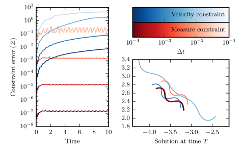
Figure 2. Convergence results in $\Delta T$ for a test problem. Left shows the error in the constraint over time $(\mathcal{Z}^{k})$ and right shows the solution $\boldsymbol{x}_{h}^{M}$ at the final time. The colours are indicated by the colour bar at the top right. Red plots correspond to the measure constraint and blue plots correspond to the velocity constraint.

The model replicates expected forward locomotion behaviours over a wide range of conditions and parameter values

To explore the dependence of the model on parameters, we ask, first, whether model implementation with default parameters from the literature (Table 1) can replicate reported locomotion behaviours. To simulate forward locomotion, we set the muscle activation function $\beta$ to be given in dimensional form by a travelling sine-wave with a decaying amplitude

(17) $$\beta(u,t) =\beta_{0}(u)\sin(2\pi uL/\lambda-2\pi\omega t),$$

$$\beta_{0}(u) =\big{(}10(1-u)+6u\big{)}\,\mathrm{mm}^{-1},\,\lambda=0.65\,\mathrm{mm},\,\omega=0.30\,\mathrm{s}^{-1}.$$

where $u$ follows a material point along the worm (varying from 0 at the head to 1 in the tail). The choice of $\beta_{0}$ reflects the maximum curvatures exhibited by a worm during forwards locomotion, see Boyle et al. (2012, Fig. 3, agar), and typical wavelength from during a crawling gate (Berri et al., 2009; Fang-Yen et al., 2010).

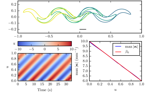
Figure 3. Simulation results for forced forward locomotion. The top panel shows simulated body postures in time, in response to crawling like muscle forcing at times $0,5,10,15\,\mathrm{s}$ (from blue to yellow). The initial condition is fixed to remove any transient behaviour. The axis are in mm with a $0.1\,\mathrm{mm}$ scale bar shown. The bottom left panel shows the travelling waves of curvature along the body. The bottom right panel shows the maximum curvature at each point along the body (after the initial transient), as compared to the muscle forcing function. Recall that $u=0$ denotes the head and $u=1$ the end of the tail.

Figure 3 features both typical body postures and a plot showing the curvature along the body for agar like external fluid forces. The postures show a near-sinosoidal configuration with curvature travelling from head to tail down the body. We see that the maximum curvature along the body follows the desired curvature imposed by the muscle forcing. In other words, as expected for agar like conditions and sufficiently high body elasticity, the passive body properties enable the body curvature to closely follow the muscle activation. Note in particular, the negligible transient time before stable undulations are observed, suggesting that the model would perform robustly in dynamics environments or under various modulations of internal or external forcing. Thus the model is able to replicate experimentally observed locomotion body postures for realistic choices of parameter values.

Next to validate the model of the linear viscoelastic environment, we test whether the thrust generated by the worm during forward locomotion agrees with reported values on agar. Simulations under agar like conditions (with a ratio of drag coefficients $K=39$) generate an absolute speed of $0.16\,\mathrm{mm}/\,\mathrm{s}$ which compares well with previously observed speeds ($0.137\pm 0.014\,\mathrm{mm}/\,\mathrm{s}$, Yemini et al. 2013).

The model performs well over a wide range parameters and body shapes

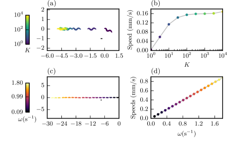
Figure 4. Modulation of the locomotion by internal and external parameters: $K$ (a,b), $\omega$ (c,d). The left column of plots (a,c) show the final shape after $28.3\,\mathrm{s}$ starting with the head at $(0,0)$. All axes are in $\,\mathrm{mm}$ with a $0.1\,\mathrm{mm}$ scale bar in the bottom right of each plot. The right column of plots (b,d) show the average speed during the trial (ignoring undulations).

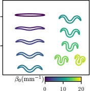
Figure 5. Simulation results for different strengths of muscle forcing $\beta_{0}$. All plots show the final shape after $33.3\,\mathrm{s}$ starting from a straight line configuration, and subject to constant forcing $\beta$. The shapes have been moved on the plot to demonstrate the different postures.

C. elegans can independently modulate its undulation frequency and waveform, within some limits. Furthermore, gait modulation (correlated across frequency and waveform) is observed as a function of the viscosity (or viscoelasticity) of the fluid environment. In our model, we are able to vary these properties independently in order to test the range of behaviours the model can generate. Figure 4(c,d) shows worms simulated with the same forcing function, but variable undulation frequencies from $0.1\,\mathrm{s}^{-1}$ to $1.8\,\mathrm{s}^{-1}$. This covers the range of parameters from Table 1. The model copes well with the full range of undulation frequencies, with the body curvature following the forcing for all. In other words, different values of $\omega$ lead to different resulting speeds but with similar body postures. By contrast, changing the wavelength of undulations $\lambda$, leads to a range of different postures as well as speeds (see Figure 7(a)). As expected, for a given waveform, for low frequencies the faster the undulation, the faster the speed. Specifically, for low values of $\omega$, we find a linear relationship between undulation frequency and forward speed, indicating that the undulation frequency merely scales the effective time of the simulation.

Next we use the model to validate behaviours across a range of external viscoelasticities by varying the ratio of drag coefficients $K$, while keeping the undulation waveform and frequency fixed. We simulated forward locomotion for $K$ ranging from 1 to 10,000. Specifically, we vary $K_{\boldsymbol{\nu}}$ whilst keeping $K_{\boldsymbol{\tau}}$ fixed. Thus an increase in $K$ corresponds to a stiffer medium. We see a lack of thrust for $K=1$, and maximum thrust for the largest values of $K$. We further find that for $K\approx 100$, the distance travelled saturates, thus increasing $K$ has a negligible effect on speed. Note for this choice of $E$, varying the ratio of environmental parameters $K\lesssim 100$ does not significantly affect the body postures in our simulations in this parameter range. This corresponds to the theory of Gray and Lissmann (1964) who that for sufficiently small undulations that the ratio $K$ dictates the forward progress per undulation (or conversely the percentage ‘slip’ relative to the background media). For $K=1$, we see total slip and for $K\sim 100$, we see minimal slip. For $K\gtrsim 1000$, the environment is too stiff for the worms muscles to overcome and less thrust is produced. Note that we expect the worm not to be able to locomote in $K\approx 1000$, which suggests that our value $E=10\,\mathrm{MPa}$ is too high (see below).

Finally, we probe the flexibility of our method in generating arbitrary body shapes. To do this, we simulate our model with similar muscle forcing function (17) but setting the amplitude of preferred undulations $\beta_{0}(u)=\beta_{0}$ to constant values from $0$-$20\,\mathrm{mm}^{-1}$. The results are shown in Figure 5. We see that as we increase $\beta_{0}$ the posture is increasingly curved. Note that for the highest value of $\beta_{0}$, the body of the worm self intersects which is not precluded from our assumptions on the fluid dynamics. This shows the highest curvatures that the model can capture. The ability to arbitrarily and reliably modulate the driving force suggests a powerful tool to study a variety of behaviours (for example, omega turns) as well as biophysical properties of muscle and cuticle over development in wild type animals, as well in animal models of disease.

4.2. Insight on nematode locomotion

The model places constraints on the range of viable material properties of the worm

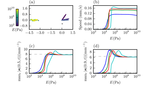
Figure 6. The effect of Young’s modulus ($E$) on locomotion. (a) The final body shape after $28.3\,\mathrm{s}$ starting with the head at $(0,0)$. Only $E$ varies. All other parameters fixed. (b) The average speed during the trial (ignoring undulations) for varying $E$ for different values of $K$ (Blue $K=10$, green $K=39$, red $K=100$, cyan $K=1000$). (c,d) Maximum curvature achieved at the centre of the body ($u=0.5$) and near the tail ($u=0.9$) for different values of $K$ (the same colours as (b)). The dashed grey line represents $\beta_{0}(u)$.

A key question is whether the key free parameter of the model, the Young’s modulus $E$, may be constrained by the model. For the above simulations, we chose a Young’s modulus of $E=10\,\mathrm{MPa}$. However the range of reported values ranges over five orders of magnitude. We therefore asked how the ability of muscle forcing to impose body curvature depends on internal elasticity. To answer this question, we repeated the above simulations varying $E$ from $1\,\mathrm{kPa}$ to $10\,\mathrm{GPa}$ with $K$ from $10$ to $1000$ (see Figure 6).

For low values of the Young’s modulus, $E$, the worm is not sufficiently stiff to overcome the external environmental stiffness which results in a large error between the curvature of the worm and the preferred curvature. The lack of generated curvature results in almost no forwards thrust. In contrast, for high values of $E$ the desired curvature is exactly achieved which leads to forwards locomotion. We note that for intermediate values of $E$, the curvature is higher than the muscle activation profile ($\beta_{0}$), which leads to even higher speeds.

The values in Table 1 list $K=39$ for agar. For $K=10$-$39$, we require that the worm’s internal elasticity suffices to generate high thrust and high curvatures. For these values, we see the transition from low to high thrust and high to low curvature difference around $E\approx 10\,\mathrm{kPa}$ (Figures 6(b,c,d) green line). We explore $K=1000$, which corresponds to $(K_{\boldsymbol{\nu}},K_{\boldsymbol{\tau}})=(3200,3.2)\cdot\,\mathrm{kg}\,\mathrm{m}^{-1}\,\mathrm{s}^{-1}$ and much larger drag than $10\,\mathrm{Pa}\,\mathrm{s}$, thus we expect to see low locomotion speeds here and for the worm to struggle to generate curvature. For $K=1000$, we see the transition from low to high thrust and high to low curvature error around $E\approx 1\,\mathrm{MPa}$ (Figures 6(b,c,d) cyan line). Combining these conservative bounds we give an estimate of $10\,\mathrm{kPa}\lesssim E\lesssim 1\,\mathrm{MPa}$.

The model suggests that the worm modulates its waveform to maintain speed

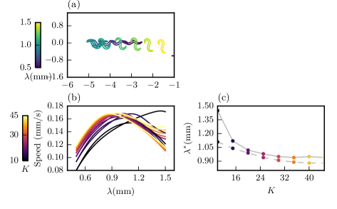
Figure 7. The undulation wavelength modulates locomotion speed. (a) The final body shape after $28.3\,\mathrm{s}$ starting with the head at $(0,0)$. Only $\lambda$ varies. All other parameters fixed. (b) The average speed during the trial (ignoring undulations) for varying $\lambda$ for different values of $K$. (c) The optimal choice of $\lambda=\lambda^{*}$ for each $K$. The solid line represents $E=10\,\mathrm{MPa}$, the dashed line represents $E=1\,\mathrm{MPa}$.

Finally we asked how wavelength modulation affects locomotion speed in different viscoelastic media. Changing the wavelength of undulations $\lambda$ (Figure 7) shows a wide range of body postures and swimming speeds. Berri et al. (2009) reported a smooth decrease of the wavelength, amplitude and frequency of undulations as the worm locomotes through increasingly resistive media, corresponding to increasing $K$. Similar forms of smooth gait modulation spanning the swim-crawl transition have also been observed for Newtonian and near-Newtonian media (Fang-Yen et al., 2010; Montenegro-Johnson et al., 2016; Lebois et al., 2012). We find that different choices of $K$ correspond to different optimal wavelengths. For agar like environments, our model yields a maximum speed for a wavelength of $\lambda_{\mathrm{opt}}(K=39)=0.9\,\mathrm{mm}$. The optimal wavelength (higher than the wavelength reported under similar conditions) appears relatively insensitive to the choice of $E$ (at $1\,\mathrm{MPa}$ and up), but depends more strongly on the choice of waveform. As $K$ is reduced, we find a that the optimal wavelength increases significantly to $\lambda_{opt}(K=10)=1.5\,\mathrm{mm}$, commensurate with a swimming wavelength (Table 1). As expected, in these low resistance environments, the optimal wavelength depends strongly on the material properties of the worm. The qualitative correspondence of the above results with the observed waveform modulation in the swim-crawl transition suggests that the worm must modulate its undulation wavelength to maximise speed across a range of environments. The simulations are repeated at $E=1\,\mathrm{MPa}$ to show qualitatively the same results, and quantitatively the similar results for sufficiently resistive environments, $K\geq 20$.

5. Discussion

In all animals, the shape of the organism is determined by integrating the effects of internal driving forces (muscle actuation) and the interaction of the passive body with its external environment. The combined action of active and passive moments in determining body shape is particularly important in the study of active swimming and undulatory locomotion, where spatio-temporal feedback about the shape of the body can stabilise the motion, facilitate adaptation and modulation of posture, and – in C. elegans – even generate the rhythmic patterns of neuromuscular activity underlying locomotion. An integrated study of locomotion in any such system requires a flexible, stable and efficient model of the biomechanics to interface to model nervous systems. To date, no such model exists.

To address this need, we have detailed a biomechanical model for undulatory locomotion of slender bodies, applied to a case study of C. elegans. The model incorporates the collective passive viscoelasticity of the tissue, an active moment, and drag forces capturing the interaction of the organism with the environment at low Reynolds numbers. In this model, the body of the worm is represented by a tapered elongated shell, driven by periodic travelling waves of muscle contraction. Effective force equations on the midline of the body are derived. While the force equations have been adapted from the literature (Landau and Lifschitz, 1975; Guo and Mahadevan, 2008), in themselves they yield an underdetermined system of equations. To close the system, we further consider conservation of mass which leads to a local length constraint. Our continuum description and closing assumption leads to a nonlinear initial-boundary value problem, which we solve for an anatomically meaningful parametrisation. Parameter values for the geometry of the body, passive and active moments, and the environmental forces are taken from anatomical and behavioural data from the literature.

Our finite element approach allows us to directly solve the non-linear system of equations and in this way differs from previous continuous models of C. elegans biomechanics (Sznitman et al., 2010a; Fang-Yen et al., 2010). This approach ensures the high accuracy and stability of the model and permits the simulations of arbitrarily large (even non-physical) curvatures. To this end, we have presented a new numerical method based on a mixed piecewise-linear piecewise-constant finite element method and semi-implicit time stepping. We have shown the robustness of the scheme analytically through a semi-discrete stability bound and good equi-distribution properties for the fully discrete scheme. Numerical experiments show the accuracy of the method. Our simulations demonstrate that the numerical methodology is robust with respect to a large variety of body shapes and has improved stability over previous articulated models (Ding et al., 2012; Boyle et al., 2012) (see in particular Boyle et al. (2012, Fig. 4C) which shows a large, behaviourally significant region of parameter space is unachievable with the authors’ approach). To our knowledge, the only other formulation of a C. elegans model with the potential to generate complex waveforms and high curvature postures relies on particle system simulations (Palyanov et al., 2016). It is our hope that the model presented here offers similar flexibility and generalisability, but with significantly lower computational overheads.

We contrast our approach with two previous approaches to computational modelling of C. elegans locomotion. First, Boyle et al. (2012) used a discrete models in which an articulated body is modelled as a repeating pattern of springs and dampers. The continuous nature of the elastic beam is particularly appealing since it more closely mimics the continuous, non-segmented body of nematodes and provides a more robust simulation framework. Second, the OpenWorm consortium (Szigeti et al., 2014) has built a cell-scale reconstruction of the worm and uses smoothed particle hydrodynamics (SPH) in order to capture physical forces (Palyanov et al., 2016). By comparison to the SPH approach, this work assumes simplified fluid dynamics and uniform density; this allows us to reduce the required number of degrees of freedom by four orders of magnitude which in turn yields a more efficient method.

The stability of the model with respect to exogenous (fluid) and endogenous (body and forcing) parameters and its ability to reliably generate dynamics with high curvature postures make it suitable for further studies of the biomechanics of this and other soft bodied systems. In particular, the choice of parametrisation provides a general framework for following material coordinates along a body (as distinct from the conventional arc-length parametrisations). In C. elegans and other side-to-side undulators in which the shape of the body is conserved locally, our formulation allows us to naturally impose the forces resulting from internal pressure. In larvae and other peristaltic undulators, distances are not locally conserved along the body, and the application of this formulation may therefore offer a powerful numerical framework for modelling similar systems.

In C. elegans, the model is particularly well suited to the study of a range of biological behaviours (e.g., locomotion, coiling and turning) and biological variants (e.g., disease models, genetic knock-out animals, developing or ageing animals) in a realistic biomechanical framework and across a wide range of Newtonian and viscoealstic physical environments that may be approximately described by drag forces. Potential examples of applications for C. elegans, where current simulators would fail include coilers, loopy worms, omega turns and more.

The model allows us, not only to generate a large range of body shapes, but also to probe relevant exogeneous and endogenous parameters of the system. In particular, our model allows us to address a long-standing open question in C. elegans: estimating the effective elasticity of the body. Our model places a estimates on the elasticity of the tissue (Young’s modulus $E\gtrsim 10\,\mathrm{kPa},E\lesssim 1\,\mathrm{MPa}$), required to overcome realistic resistive forces and generate forward thrust. These results are consistent the estimate of Backholm et al. (2013) with prior qualitative experimental observations but higher than the estimate of Sznitman et al. (2010a) and lower than the estimates of Park et al. (2007); Fang-Yen et al. (2010).

If the Young’s modulus is too low, this would restrict the behavioural repertoire of the worm. In particular, we are able to set a lower bound on the Young’s modulus by requiring that the worm can both bend and generate thrust in agar-like conditions. Conversely, we set an upper bound based on behavioural observations that the worm fails to generate thrust in sufficiently resistive environments. Intuitively, the stiffer the cuticle, the higher the power-output of the muscles required to achieve the desired bending. Furthermore, for agar like environments, the locomotion of the worm is not power limited (Berri et al., 2009). However, resistive force theory suggests that the worm must considerably increase its muscle power to navigate through increasingly resistive media so that at sufficiently high viscosity or viscoelasticity, power limitations dominate. Thus, it is not known whether a higher Young’s modulus may incur a prohibitive material cost, a prohibitive muscle power, or whether such high viscoelasticity environments are sufficiently rare in the worm’s natural habitat to preclude such a need. Finally, we show that for a given choice of Young’s modulus, waveform modulation allows worms to optimise speed as they maneuvre through different viscous and viscoelastic environments.

Combined, the generality of the model and combination of analysis and numerical simulations that demonstrate the good properties of our method, suggest broad applicability for the simulation of locomotory behaviours in non-segmented soft-bodied systems and predictions of not only body shapes but also swimming speeds. Future extensions of the numerical scheme include effectively capturing internal viscosity. This will allow the model to also be used in lower resistance environments and, for example, capture in more detail the transition from crawling to swimming.

This work focuses on the biomechanical aspects of locomotion and stops short of integrating the dynamics of the nervous system which is responsible for the rhythmic control that activates the muscles, and thus generates the locomotion. Instead, we use prescribed muscle activation functions similarly to Sznitman et al. (2010a) to actuate the passive body. Our formulation of the model lays the ground for a robust and efficient integration of closed-loop control including nervous system, body and environment. The efficiency and stability displayed by this numerical approach suggest that an appropriate integrated approach, including neuromuscular control and proprioceptive feedback could make predictions about non-undulatory behaviours such as complex navigation and motion through granular or heterogeneous environments.

References

-
Backholm et al. (2015a)
Backholm, M., Kasper, A. K. S., Schulman, R. D., Ryu, W. S., Dalnoki-Veress,
K., sep 2015a. The effects of viscosity on the undulatory
swimming dynamics of C. elegans. Physics of Fluids 27 (9), 091901.
URL http://dx.doi.org/10.1063/1.4931795 -