Convergence analysis of an explicit splitting method for laser plasma interaction simulations

Abstract

Convergence of a triple splitting method originally proposed in TuePLH10 ; Lil10 for the solution of a simple Vlasov-Maxwell system, that describes laser plasma interactions with overdense plasmas, is analyzed. For classical explicit integrators it is the large density parameter that would impose a restriction on the time step size to make the integration stable. The triple splitting method contains an exponential integrator in its central component and was specifically designed for systems that describe laser plasma interactions and overcomes this restriction. We rigorously analyze a slightly generalized version of the original method. This analysis enables us to identify modifications of the original scheme, such that a second order convergent scheme is obtained.

1 Introduction

We consider the numerical solution of a simplified Vlasov-Maxwell system of equations, describing laser plasma interactions with an overdense plasma. After discretizing in space for a fixed spatial grid parameter $\Delta x$ a system of ordinary differential equations is obtained. The situation we wish to consider now is slightly unusual as it is the overdense plasma and not the space discretization that gives rise to fast oscillations in the solution. And hence it would be the plasma frequency that would impose a step size restriction in explicit Runge-Kutta or multistep methods. To overcome the restriction on the time step size due the plasma frequency a triple splitting method with filter functions was introduced by Liljo and Tückmantel, Pukhov, Liljo and Hochbruck in Lil10 ; TuePLH10 for this model problem. An astute choice of filter functions results in a method that shows excellent behavior in numerical experiments. Numerical experiments in TuePLH10 indicate convergence of second order in the time step size $\tau$ independent of the plasma density $\rho$. A more detailed experiment, which is reported in Section 8.1, reveals that the method from TuePLH10 is not second order in $\tau$ independent of the plasma density $\rho$, but is merely stable.

By our convergence analysis of the triple splitting we are able to formulate conditions on the filter functions to obtain second order convergence in $\tau$ independent of the plasma density $\rho$. These conditions can be fulfilled by slightly modifying the choice of the filter functions originally proposed in Lil10 ; TuePLH10 .

As the triple splitting is an explicit integrator the method certainly can not be expected to be convergent uniformly in $\Delta x\to 0$. Thus our aim here is to prove convergence independent of the large plasma density $\rho$ but not independent of the spatial discretization parameter $\Delta x$.

In a nutshell the plan for the convergence proof is as follows: The triple splitting for the impulse of the plasma density $\mathbf{p}$, the electric field $\mathbf{e}$ and the magnetic flux $\mathbf{b}$ will be reformulated as a two step method for $\mathbf{e}$ only with some sort of “natural” filter. Perturbing the initial values this reformulation allows to estimate the error in $\mathbf{e}$ using a result from Hairer, Lubich and Wanner (HaiLW06, , Theorem XIII.4.1). We then show that the perturbation in the initial values is small enough, such that by a stability argument convergence for $\mathbf{e}$ is obtained. The estimates for the magnetic flux $\mathbf{b}$ and the impulse $\mathbf{p}$ are obtained by a judicious combination of ideas borrowed from Grimm and Hochbruck GriH06 with trigonometric identities. The present paper is based on the first part of the PhD thesis Jan15 .

2 Physical problem and spatial discretization

Consider the propagation of a short laser pulse in vacuum targeted at a plasma around a thin foil. The electric field $\mathbf{e}$ and the magnetic flux $\mathbf{b}$ describing the laser are governed by Maxwell’s equations. In this simple model the plasma is modeled as a fluid by the electron number density $\rho$ (number of electrons per volume) and the probability density function of the impulses of the electrons $\mathbf{p}$. The laser plasma interactions with an overdense plasma ($\rho\gg 1$) and a linear response of the plasma to the laser is modeled by

$$\partial_{t}\mathbf{p} =\mathbf{e}, x\in B,t>0,$$ (1a)

$$\partial_{t}\mathbf{e} =\nabla\times\mathbf{b}-f^{2}\rho\mathbf{p}, x\in B,t>0,$$ (1b)

$$\partial_{t}\mathbf{b} =-\nabla\times\mathbf{e}, x\in B,t>0.$$ (1c)

Here $f=2\pi e$, where $e$, the electron charge, is a constant. $B$ is the computational domain, a box, containing the plasma and the support of the initial values. The vacuum permittivity (electric constant) and permeability (magnetic constant) are set to $1$. In our simplified model plasma only oscillates locally, thus its impulses $\mathbf{p}$ also oscillate, but the density $\rho$, remains constant. There are two further essential assumptions. We assume that the electrons move slowly, such that relativistic effects can be neglected, i.e. the velocity field of the plasma $\mathbf{v}$ is proportional to the impulse $\mathbf{p}$. Secondly we neglect the magnetic Lorentz force $\mathbf{v}\times\mathbf{b}$. These rather restrictive assumptions make the model (1) linear. A more detailed derivation of the model may be found in TuePLH10 ; Tue13 .

Equation (1) has to be supplemented with boundary conditions and initial values. The theory developed below applies to the case of perfect magnetic conductor (PMC), perfect electric conductor (PEC) or periodic boundary conditions, which guarantee that the “curl curl” operator is self-adjoint HipKT12 .

As we only discuss the convergence of the semi-discrete problem in the following, the solution of the spatially discretized equations will again be denoted by $\mathbf{p}$, $\mathbf{e}$ and $\mathbf{b}$. Discretizing in space with the Yee scheme or curl-conforming finite elements we denote by $\mathbf{C}_{E}$ and $\mathbf{C}_{B}$ discrete versions of the “curl” applied to $\mathbf{e}$ and $\mathbf{b}$ respectively. Note that these curl-operators are allowed to be different and should be different. The electric field $\mathbf{e}$ can conveniently be interpreted as a differential $1$-form, then $\mathbf{C}_{E}$ is a discrete version of “curl”. Whereas in this context $\mathbf{b}$ has to be interpreted as differential $2$-form, such that $\mathbf{C}_{B}$ is as discrete version of “*curl*”, where * is the Hodge operator Hip02 .

The multiplication with $f^{2}\rho$ is discretized by a matrix $\mathbf{\Omega}^{2}$. In case of the Yee scheme $\mathbf{\Omega}^{2}$ is a diagonal matrix. In case one uses curl-conforming finite elements, $\mathbf{\Omega}^{2}$ is a positive semidefinite matrix and mass matrices arise on the right hand side of (1). In what follows we will assume that $\mathbf{\Omega}^{2}$ is a diagonal matrix with only one positive eigenvalue. Generalizations to a non-diagonal but symmetric positive semidefinite discretization $\mathbf{\Omega}^{2}$ of the multiplication operator will be discussed in Section 7.

If space is scaled to the wave number and time to the laser frequency the spatially discretized equations are

$$\partial_{t}\mathbf{p} =\mathbf{e}, t>0,$$ (2a)

$$\partial_{t}\mathbf{e} =\mathbf{C}_{B}\mathbf{b}-\mathbf{\Omega}^{2}\mathbf{p}, t>0,$$ (2b)

$$\partial_{t}\mathbf{b} =-\mathbf{C}_{E}\mathbf{e}, t>0.$$ (2c)

Assuming for the moment that $\rho$ vanishes, a right traveling pulse with width parameter $\sigma_{0}=10$ and wavelength $1$ solving (1) is given by

$$\mathbf{e}_{y}=\mathbf{b}_{z}=a_{0}\exp\left(-\frac{(2\pi[(x-\bar{x})-t])^{2}}{2\sigma_{0}^{2}}\right)\cos(2\pi[(x-\bar{x})-t]),$$ (3)

$$\mathbf{e}_{x}\equiv\mathbf{e}_{z}\equiv\mathbf{b}_{x}\equiv\mathbf{b}_{y}\equiv 0.$$

If we set $t=0$, $\bar{x}=10$ and $a_{0}=1$ in (3) initial values for a pulse centered at $10$ with amplitude $1$ are obtained.

The plasma is located away from the initial location of the pulse by choosing $\rho=10^{8}$ for $x\in[20,21]$ and $\rho=0$ elsewhere. This leads to a total reflection of the laser pulse on the edge of the plasma. Figure 1 shows different snap shots of the simulation.

Figure 1: Solution of (1) with the laser pulse from (3) as initial value. Impulse $\mathbf{p}_{y}$ (green), electric field $\mathbf{e}_{y}$ (red), magnetic flux $\mathbf{b}_{z}$ (blue) and electron density $\rho$ (magenta) scaled to one. First graphic ($t=0$): Initial data, second ($t=5$): propagation of the pulse in vacuum, third ($t=10$): total reflection at the foil, fourth ($t=20$): back propagation

3 Numerical scheme and filter functions

To solve the spatially discretized equations (2) we use the triple splitting method proposed by Liljo and Tückmantel, Pukhov, Liljo and Hochbruck in Lil10 ; TuePLH10 . To this end the right hand side is split into three terms

$$\partial_{t}\left[~{}\begin{matrix}\mathbf{p}\\ \mathbf{e}\\ \mathbf{b}\end{matrix}~{}\right] =\left[~{}\begin{matrix}0\\ 0\\ -\mathbf{C}_{E}\mathbf{e}\end{matrix}~{}\right] + \left[~{}\begin{matrix}0\\ \mathbf{C}_{B}\mathbf{b}\\ 0\end{matrix}~{}\right] + \left[~{}\begin{matrix}0&1\\ -\mathbf{\Omega}^{2}&0\\ &&0\end{matrix}~{}\right]\left[~{}\begin{matrix}\mathbf{p}\\ \mathbf{e}\\ \mathbf{b}\end{matrix}~{}\right]:=f_{1}+f_{2}+f_{3}.$$

The fully discrete scheme is a symmetric triple splitting obtained by taking the exact flows of the split equations (i.e. with only one $f_{i}$ as right hand side) as propagators. As already observed in Lil10 ; TuePLH10 due to resonances this is not sufficient for convergence independent of $\rho$. To introduce filter functions is a widely used mean to avoid resonance effects, see e.g. Garcia-Archilla1998 ; HocL99 ; Hairer2001 ; GriH06 ; HaiLW06 . We follow Lil10 ; TuePLH10 , introduce filter functions symmetrically and obtain the following numerical scheme

$$\mathbf{b}_{n+\frac{1}{2}} =\mathbf{b}_{n}-\tfrac{\tau}{2}{\color[rgb]{0,0,1}\psi_{B}(\tfrac{\tau}{2}\mathbf{\Omega})}\mathbf{C}_{E}{\color[rgb]{0.2,0.5,0.02}\phi_{E}(\tfrac{\tau}{2}\mathbf{\Omega})}\mathbf{e}_{n},$$ (4a)

$$\mathbf{e}_{n}^{+} =\mathbf{e}_{n}+\tfrac{\tau}{2}{\color[rgb]{0.2,0.5,0.02}\psi_{E}(\tfrac{\tau}{2}\mathbf{\Omega})}\mathbf{C}_{B}{\color[rgb]{0,0,1}\phi_{B}(\tfrac{\tau}{2}\mathbf{\Omega})}\mathbf{b}_{n+\frac{1}{2}},$$ (4b)

$$\left[~{}\begin{matrix}\mathbf{p}_{n+1}\\ \mathbf{e}_{n+1}^{-}\end{matrix}~{}\right] =\left[~{}\begin{matrix}\cos(\tau\mathbf{\Omega})&\tau\operatorname{sinc}(\tau\mathbf{\Omega})\\ -\mathbf{\Omega}\sin(\tau\mathbf{\Omega})&\cos(\tau\mathbf{\Omega})\\ \end{matrix}~{}\right]\left[~{}\begin{matrix}\mathbf{p}_{n}\\ \mathbf{e}_{n}^{+}\end{matrix}~{}\right],$$ (4c)

$$\mathbf{e}_{n+1} =\mathbf{e}_{n+1}^{-}+\tfrac{\tau}{2}{\color[rgb]{0.2,0.5,0.02}\psi_{E}(\tfrac{\tau}{2}\mathbf{\Omega})}\mathbf{C}_{B}{\color[rgb]{0,0,1}\phi_{B}(\tfrac{\tau}{2}\mathbf{\Omega})}\mathbf{b}_{n+\frac{1}{2}},$$ (4d)

$$\mathbf{b}_{n+1} =\mathbf{b}_{n+\frac{1}{2}}-\tfrac{\tau}{2}{\color[rgb]{0,0,1}\psi_{B}(\tfrac{\tau}{2}\mathbf{\Omega})}\mathbf{C}_{E}{\color[rgb]{0.2,0.5,0.02}\phi_{E}(\tfrac{\tau}{2}\mathbf{\Omega})}\mathbf{e}_{n+1}.$$ (4e)

For $i\in\{E,B\}$ we require $\psi_{i}$, $\phi_{i}$ to be even, analytic functions such that $\psi_{i}(z),\phi_{i}(z)\to 1$ for $z\to 0$.

In the following section we state assumptions on the physical data and the spatial discretization that are necessary for the convergence proof.

4 Assumptions

The following assumptions are not too restrictive from a theoretical physics point of view. They are fulfilled for example in the situation considered in Lil10 ; TuePLH10 simulating the reflection of a laser pulse by a plasma.

Assumption 1

We assume that

1. the product $\mathbf{C}_{B}\mathbf{C}_{E}=:-\mathbf{G}=-\mathbf{G}^{T}$ is symmetric, positive semidefinite,

2. $\mathbf{\Omega}$ is a diagonal matrix given by

   $$\mathbf{\Omega}=\left[~{}\begin{matrix}0&0\\ 0&\widetilde{\omega}\operatorname{Id}\end{matrix}~{}\right],\qquad\widetilde{\omega}\gg 1$$ (5)

   and

3.  
   

   $$\|\mathbf{C}_{E}\|\leq C_{c},\ \text{and}\ \|\mathbf{C}_{B}\|\leq C_{c},\quad\text{such that}\quad\|\mathbf{G}\|\leq C_{g}:=C_{c}^{2}$$ (6)

   for a constant $C_{c}$ independent of $\widetilde{\omega}$.

The symmetry and negative semi-definiteness of $\mathbf{G}$ comes quite natural, provided that the continuous “curl curl” operator is self-adjoint and positive semi-definite, which is the case for appropriate boundary conditions such as perfect electric conductor (PEC), perfect magnetic conductor (PMC) or periodic boundary conditions, see HipKT12 . Condition (5) implies that the matrix $\mathbf{\Omega}$ has only one (large) non-zero eigenvalue $\widetilde{\omega}>0$. In our case it is given by the density parameter, i.e. $\widetilde{\omega}=f\sqrt{\rho}$. This is an essential restriction, which is only needed in the proof of Theorem 6.2. A modification of our proof, that only requires $\mathbf{\Omega}$ to be symmetric positive semi-definite, is given by Buchholz and Hochbruck in BucH15 and will be discussed in Section 7. Estimates (6) imply that we do not obtain error bounds uniformly in the spatial discretization parameter, e.g. the mesh width. As mentioned already in the introduction this would indeed be impossible for our integration scheme since it reduces to the Störmer-Verlet method in case of no material ($\rho\equiv 0$), which is known to be conditionally stable only. Assumption 1 is for example satisfied if the curl operators with periodic boundary conditions are discretized using a Yee-scheme and a step function $\rho$ is evaluated point-wise.

Additionally we need some bounds on the initial data $\mathbf{e}_{0},\mathbf{b}_{0}$ and $\mathbf{p}_{0}$ to obtain stable solutions as discussed in Section 6.1:

Assumption 2

We assume that

$$\|\mathbf{\Omega}\mathbf{e}_{0}\|^{2}\leq\tfrac{2}{3}H_{0},\quad\|\mathbf{C}_{B}\mathbf{b}_{0}\|^{2}\leq\tfrac{1}{3}\min\{1,\tfrac{4}{C_{4}^{2}}\}H_{0},\quad\|\mathbf{\Omega}^{2}\mathbf{p}_{0}\|^{2}\leq\tfrac{1}{3}H_{0},$$ (7)

$$-\left<\mathbf{e}_{0},\mathbf{G}\mathbf{e}_{0}\right>=\|\mathbf{C}_{E}\mathbf{e}_{0}\|^{2}\leq 2H_{0},\qquad\|\mathbf{e}_{0}\|^{2}\leq H_{0},$$ (8)

$$\|\mathbf{b}_{0}\|^{2}\leq H_{0}\quad\mbox{and}\quad\|\mathbf{\Omega}^{2}\mathbf{C}_{B}\mathbf{b}_{0}\|^{2}\leq H_{0},$$ (9)

for constants $H_{0}$ and $C_{4}$ independent of $\widetilde{\omega}$.

A bound with respect to multiplication with $\mathbf{\Omega}$ implies, that the initial data are sufficiently far away from the plasma, such that the product of the field strength and the density is bounded independent of the density. Bounds with respect to multiplications with $\mathbf{C}_{B}$ or $\mathbf{C}_{E}$ maybe seen as smoothness conditions for the initial data.

5 Main theorem

For our convergence result we need conditions on the filter functions, which we collect below. As in TuePLH10 we require

$$\phi_{B}\equiv\psi_{B}\equiv 1.$$ (10)

The following bounds for the filter functions are required for second order convergence of the scheme (4)

$$|(\cos(z)+1)\psi_{E}(\tfrac{1}{2}z)| \leq C_{1}\operatorname{sinc}^{2}(\tfrac{1}{2}z),$$ (11a)

$$|\phi_{E}(\tfrac{1}{2}z)| \leq C_{2}|\operatorname{sinc}(\tfrac{1}{2}z)|,$$ (11b)

$$|(\cos(z)+1)\psi_{E}(\tfrac{1}{2}z)\phi_{E}(\tfrac{1}{2}z)| \leq C_{3}|\operatorname{sinc}(z)|,$$ (11c)

$$|(\cos(z)+1)\psi_{E}(\tfrac{1}{2}z)| \leq C_{4}|\operatorname{sinc}(z)|,$$ (11d)

$$\left|\operatorname{sinc}(z)-\tfrac{1}{2}(\cos(z)+1)\psi_{E}(\tfrac{1}{2}z)\right| \leq C_{5}z^{2}|\operatorname{sinc}(z)|,$$ (11e)

$$|\operatorname{sinc}(z)-\phi_{E}(\tfrac{1}{2}z)| \leq C_{6}|z\sin(\tfrac{1}{2}z)|,$$ (11f)

$$|\psi_{E}(z)| \leq C_{7}$$ (11g)

and

$$|\operatorname{sinc}^{2}(\tfrac{1}{2}z)-\operatorname{sinc}(z)\phi_{E}(\tfrac{1}{2}z)| \leq C_{8}\sin^{2}(\tfrac{1}{2}z).$$ (11h)

With these conditions we obtain our main result

Theorem 5.1

Let $\mathbf{C}_{B},\mathbf{C}_{E}$ and $\mathbf{\Omega}$ be such that Assumption 1 is fulfilled. Consider the numerical solution of the system (2) by the splitting method (4) with time step size $\tau$ satisfying $\tau\leq\tau_{0}$, for sufficiently small $\tau_{0}$ independent of $\widetilde{\omega}$ with $\tau\widetilde{\omega}\geq c_{0}>0$. If the initial values satisfy conditions (7) to (9) with a constant $H_{0}$ independent of $\widetilde{\omega}$ and the filter functions satisfy (11a)-(11h) then for $t_{n}:=t_{0}+n\tau\leq T$ we obtain the following second order estimates for the errors

$$\|\mathbf{p}_{n}-\mathbf{p}(t_{n})\|\leq C\tau^{2},\quad\|\mathbf{e}_{n}-\mathbf{e}(t_{n})\|\leq C\tau^{2},\quad\|\mathbf{b}_{n}-\mathbf{b}(t_{n})\|\leq C\tau^{2}.$$ (12)

The constant $C$ is independent of  $\widetilde{\omega}$, $\tau$, $n$ or derivatives of the solution, but depends on $(T-t_{0})$ and the constants $C_{1},...,C_{8}$ and $C_{c}$ in (6) and $H_{0}$.

The assumption $\tau\widetilde{\omega}\geq c_{0}>0$ is the interesting case and is no restriction as otherwise we are in the case of classical convergence analysis. The proof is given in Section 6.

Choice of the filter functions

Tückmantel et. al. TuePLH10 propose the choice

$$\phi_{E}=\psi_{E}=z\mapsto\operatorname{sinc}(z),\qquad\phi_{B}\equiv\psi_{B}\equiv 1,$$ (13)

which satisfies conditions (11b) to (11h). It does not obey condition (11a) but only the weaker estimate $|(\cos(z)+1)\psi_{E}(\tfrac{1}{2}z)|\leq C_{0}\operatorname{sinc}(\tfrac{1}{2}z)$. Detailed numerical tests in Section 8.1 for this choice reveal sharp resonances a even multiples of $\pi/\omega$, which where not observed in TuePLH10 .

We propose the new choice

$$\phi_{E}=z\mapsto\operatorname{sinc}(z),\qquad\psi_{E}=z\mapsto\operatorname{sinc}^{2}(z),\qquad\phi_{B}\equiv\psi_{B}\equiv 1,$$ (14)

which also statisfies the first filter condition (11a) and thus by Theorem 5.1 results in second order error bounds. The detailed proof that the filter functions (14) meet all of conditions (11) can be found in (Jan15, , Section 4.12).

These two choices of filter functions are used on the numerical experiment in Section 8.1. Figure 2 there shows the error for the scheme (4), without filter (None), with the filter choice (14) (New), which yields a second order scheme uniformly in $\omega$, and with the filter choice (13) (Orig) which violates (11a) and shows sharp resonances and a breakdown of the method if $\tau\widetilde{\omega}$ is close to even multiples of $\pi$.

Remark 1

Theorem 4.19 of Jan15 claims that for the filter choice (13) one obtains convergence of order one in $\tau$ independent of $\omega$. This however is shown to be wrong by our numerical tests in Section 8.1. Theorem 4.19 of Jan15 was derived in an analogous way to the second order result presented below. It is based on a supplementary first order convergence result for the two step method (22) given in (HaiLW06, , Theorem XIII.4.1) for the weakened filter assumption $|(\cos(z)+1)\psi_{E}(\tfrac{1}{2}z)|\leq C_{0}\operatorname{sinc}(\tfrac{1}{2}z)$ replacing (11a), see also Remark 2 below.

6 Proof of Theorem 5.1

The proof is divided into four steps. First we reformulate the scheme (4) as a two step method for the electric field $\mathbf{e}$ only. With this reformulation we can apply an already known error estimate to control the error in the electric field after modifying the intitial values. Based on the error bound for $\mathbf{e}$ error bounds for $\mathbf{b}$ and $\mathbf{p}$ are obtained. A more detailed proof can be found in (Jan15, , Chapter 4).

6.1 Reformulation

From equation (2) one obtains an equation for electric field

$$\partial_{tt}\mathbf{e}(t)=-\mathbf{\Omega}^{2}\mathbf{e}(t)+\mathbf{G}\mathbf{e}(t),$$ (15a)

$$\mathbf{e}(t_{0})=\mathbf{e}_{0},\quad\partial_{t}\mathbf{e}(t_{0})=\mathbf{C}_{B}\mathbf{b}(t_{0})-\mathbf{\Omega}^{2}\mathbf{p}(t_{0}):=\dot{}\mathbf{e}_{0}$$ (15b)

with Hamiltonian

$$\mathcal{H}(\mathbf{e},\mathbf{f})=\tfrac{1}{2}\|\mathbf{f}\|^{2}+\tfrac{1}{2}\|\mathbf{\Omega}\mathbf{e}\|^{2}-\tfrac{1}{2}\left<\mathbf{e},\mathbf{G}\mathbf{e}\right>=\tfrac{1}{2}\|\mathbf{f}\|^{2}+\tfrac{1}{2}\|\mathbf{\Omega}\mathbf{e}\|^{2}+\tfrac{1}{2}\|\mathbf{C}_{E}\mathbf{e}\|^{2}.$$ (16)

From Assumption 2 we deduce the stability estimates

$$\mathcal{H}(\mathbf{e}(t),\partial_{t}\mathbf{e}(t)) \leq 2H_{0},$$ (17)

$$\|\mathbf{e}(t)\| \leq(1+2(T-t_{0}))\sqrt{H_{0}},$$ (18)

$$\|\mathbf{b}(t)\| \leq(1+2(T-t_{0}))\sqrt{H_{0}}$$ (19)

for $t_{0}\leq t\leq T$. The latter two can be obtained by expressing $\mathbf{e}(t)$ and $\mathbf{b}(t)$ with the fundamental theorem of calculus and exploiting that the integrands $\partial_{t}\mathbf{e}$ and $-\mathbf{C}_{E}\mathbf{e}$ are both bounded by the Hamiltonian. The variation of constants formula gives the following representation of the solution $\mathbf{e}$ of (15b) starting from $t^{\prime}$ with initial data $\mathbf{e}(t^{\prime})$ and $\partial_{t}\mathbf{e}(t^{\prime})$

$$\mathbf{e}(t)= \cos((t-t^{\prime})\mathbf{\Omega})\mathbf{e}(t^{\prime})+(t-t^{\prime})\operatorname{sinc}((t-t^{\prime})\mathbf{\Omega})\partial_{t}\mathbf{e}(t^{\prime})$$

$$+(t-t^{\prime})\int_{0}^{1}(t-t^{\prime})(1-\xi)\operatorname{sinc}((t-t^{\prime})(1-\xi)\mathbf{\Omega})\mathbf{G}\mathbf{e}(t^{\prime}(1-\xi)+t\xi)\operatorname{d}\!\xi$$ (20)

and similar for $$\partial_{t}\mathbf{e}$$

$$\partial_{t}\mathbf{e}(t)= -\mathbf{\Omega}\sin((t-t^{\prime})\mathbf{\Omega})\mathbf{e}(t^{\prime})+\cos((t-t^{\prime})\mathbf{\Omega})\partial_{t}\mathbf{e}(t^{\prime})$$

$$+(t-t^{\prime})\int_{0}^{1}\cos((t-t^{\prime})(1-\xi)\mathbf{\Omega})\mathbf{G}\mathbf{e}(t^{\prime}(1-\xi)+t\xi)\operatorname{d}\!\xi.$$ (21)

For an $\mathbf{e}$-only formulation for the numerical scheme, we use (4a), (4b) and (4c) to eliminate $\mathbf{b}_{n+1},\mathbf{e}_{n}^{+}$ and $\mathbf{e}_{n+1}^{-}$ from (4d)

$$\mathbf{e}_{n+1} =-\mathbf{\Omega}\sin(\tau\mathbf{\Omega})\mathbf{p}_{n}+\cos(\tau\mathbf{\Omega})\mathbf{e}_{n}+\tau\tfrac{1}{2}(\cos(\tau\mathbf{\Omega})+\operatorname{Id})\psi_{E}(\tfrac{\tau}{2}\mathbf{\Omega})\mathbf{C}_{B}\phi_{B}(\tfrac{\tau}{2}\mathbf{\Omega})\mathbf{b}_{n}$$

$$\qquad\qquad+\tau^{2}\tfrac{1}{4}(\cos(\tau\mathbf{\Omega})+\operatorname{Id})\psi_{E}(\tfrac{\tau}{2}\mathbf{\Omega})\mathbf{C}_{B}\phi_{B}(\tfrac{\tau}{2}\mathbf{\Omega})\psi_{B}(\tfrac{\tau}{2}\mathbf{\Omega})\mathbf{C}_{E}\phi_{E}(\tfrac{\tau}{2}\mathbf{\Omega})\mathbf{e}_{n}.$$

The filter functions $\psi_{i},\phi_{i}$, $i\in\{E,B\}$ are even and hence the matrix-functions that are applied to $\mathbf{p}_{n}$ and $\mathbf{b}_{n}$ are uneven as functions of $\tau$, whereas the matrix-functions that are applied to $\mathbf{e}_{n}$ are even in $\tau$. This observation results in the two step formulation

$$\mathbf{e}_{n+1}-2\cos(\tau\mathbf{\Omega})\mathbf{e}_{n}+\mathbf{e}_{n-1}$$

$$\qquad\qquad=\tau^{2}\tfrac{1}{2}(\cos(\tau\mathbf{\Omega})+\operatorname{Id})\psi_{E}(\tfrac{\tau}{2}\mathbf{\Omega})\mathbf{C}_{B}\phi_{B}(\tfrac{\tau}{2}\mathbf{\Omega})\psi_{B}(\tfrac{\tau}{2}\mathbf{\Omega})\mathbf{C}_{E}\phi_{E}(\tfrac{\tau}{2}\mathbf{\Omega})\mathbf{e}_{n}$$

To obtain a formulation close to the two step form of (HaiLW06, , Chapter XIII) we use (10) and get rid of the filter functions “between” the two curl operators

$$\mathbf{e}_{n+1}-2\cos(\tau\mathbf{\Omega})\mathbf{e}_{n}+\mathbf{e}_{n-1} =\tau^{2}\tfrac{1}{2}(\cos(\tau\mathbf{\Omega})+\operatorname{Id})\psi_{E}(\tfrac{\tau}{2}\mathbf{\Omega})\mathbf{G}\phi_{E}(\tfrac{\tau}{2}\mathbf{\Omega})\mathbf{e}_{n}.$$ (22)

Again with (10) the equations for $\mathbf{b}$ and $\mathbf{p}$ of the numerical scheme finally read

$$\mathbf{p}_{n+1} =\cos(\tau\mathbf{\Omega})\mathbf{p}_{n}+\tau\operatorname{sinc}(\tau\mathbf{\Omega})\mathbf{e}_{n}+\tau^{2}\tfrac{1}{2}\operatorname{sinc}(\tau\mathbf{\Omega})\psi_{E}(\tfrac{\tau}{2}\mathbf{\Omega})\mathbf{C}_{B}\mathbf{b}_{n}$$

$$\qquad-\tau^{3}\tfrac{1}{4}\operatorname{sinc}(\tau\mathbf{\Omega})\psi_{E}(\tfrac{\tau}{2}\mathbf{\Omega})\mathbf{G}\phi_{E}(\tfrac{\tau}{2}\mathbf{\Omega})\mathbf{e}_{n},$$ (23)

and

$$\mathbf{b}_{n+1} =\mathbf{b}_{n}-\tau\tfrac{1}{2}\mathbf{C}_{E}\phi_{E}(\tfrac{\tau}{2}\mathbf{\Omega})\left(\mathbf{e}_{n}+\mathbf{e}_{n+1}\right)\!.$$ (24)

6.2 Error in the electric field

We want to apply Theorem 4.1 (HaiLW06, , Chapter XIII) to estimate the error in the electric field. Unfortunately this requires a distinct first time step, that our scheme (4) does not fulfill. To circumvent this problem we perturb the initial value for the derivative of the $\mathbf{e}$-field, which then yields the correct scheme. For an estimate with the original initial values we use a stability estimate for the exact solution.

The following theorem restates (HaiLW06, , Theorem XIII.4.1) adapted to the situation at hand.

Theorem 6.1

Let $\mathbf{\Omega}$ and $\mathbf{G}$ be as in Assumption 1. Consider the solution of equation (15a) for the electric field by method (22) with step size $\tau\leq\tau_{0}$ for a sufficiently small $\tau_{0}$ independent of $\widetilde{\omega}$ with $\tau\widetilde{\omega}\geq c_{0}>0$. We denote the exact solution by $\mathbf{e}\,\!^{\prime}(t)$, and the numerical solution by $\mathbf{e}_{n}\,\!^{\prime}$. The first time step is computed via

$$\mathbf{e}_{1}\,\!^{\prime}=\cos(\tau\mathbf{\Omega})\mathbf{e}_{0}\,\!^{\prime}+\tau\operatorname{sinc}(\tau\mathbf{\Omega})\dot{\mathbf{e}}_{0}\,\!^{\prime}+\tau^{2}\tfrac{1}{4}(\cos(\tau\mathbf{\Omega})+\operatorname{Id})\psi_{E}(\tfrac{\tau}{2}\mathbf{\Omega})\mathbf{G}\phi_{E}(\tfrac{\tau}{2}\mathbf{\Omega})\mathbf{e}_{0}\,\!^{\prime},$$ (25)

where

$$\mathbf{e}_{0}\,\!^{\prime}:=\mathbf{e}_{0},\ \text{ and }\ \dot{\mathbf{e}}_{0}\,\!^{\prime}:=\chi(\tau\mathbf{\Omega})\mathbf{C}_{B}\mathbf{b}_{0}-\mathbf{\Omega}^{2}\mathbf{p}_{0}$$ (26)

with

$$\chi(z):=\tfrac{1}{2}\frac{\cos(z)+1}{\operatorname{sinc}(z)}\psi_{E}(\tfrac{1}{2}z)$$ (27)

and $\mathbf{e}_{0}$ and $\mathbf{b}_{0}$ and $\mathbf{p}_{0}$ are such that conditions (7) hold true.

If conditions (11a), (11b), (11c) and (11d) are satisfied with constants independent of $\widetilde{\omega}$ for the even entire filter functions $\psi_{E},\phi_{E}:\mathbb{R}_{\geq 0}\to\mathbb{R}$ with $\psi_{E}(0)=\phi_{E}(0)=1$ we obtain

$$\|\mathbf{e}_{n}\,\!^{\prime}-\mathbf{e}\,\!^{\prime}(t_{n})\|\leq C\tau^{2}\qquad\textup{for}\qquad t_{n}:=t_{0}+n\tau\leq T$$

with a constant $C$ independent of $n$, $\tau$ and $\tilde{\omega}$ but depending on the $(T-t_{0})$ and the constants $H_{0}$, $C_{g}$ and $C_{1},...,C_{3}$.

Proof

The filter functions of (HaiLW06, , Theorem XIII.4.1) are

$$\psi(z):=\tfrac{1}{2}(\cos(z)+1)\psi_{E}(\tfrac{1}{2}z),\qquad\phi(z):=\phi_{E}(\tfrac{1}{2}z),\forall~{}z\in\mathbb{C}.$$ (28)

As $\mathbf{G}$ is symmetric we can write $\mathbf{G}\mathbf{e}=\nabla U(\mathbf{e})$ with $U=\tfrac{1}{2}\mathbf{e}^{T}\mathbf{G}\mathbf{e}$. From condition (11d) we obtaion that $\chi$ is bounded by $C_{4}$. The factor $4/C_{4}^{2}$ in the estimate for $\mathbf{C}_{B}\mathbf{b}_{0}$ in (7) guaranties the estimate for the initial oscillatory energy for the perturbed initial values. Hence all assumptions of (HaiLW06, , Theorem XIII.4.1) are fulfilled and its application completes the proof. ∎

Remark 2

In (HaiLW06, , Theorem XIII.4.1) it is claimed that one would obtain

$$\|\mathbf{e}_{n}\,\!^{\prime}-\mathbf{e}\,\!^{\prime}(t_{n})\|\leq C\tau,$$

if only the weaker estimate $|\psi(z)|\leq C_{0}|\operatorname{sinc}(\tfrac{1}{2}z)|$ instead of $|\psi(z)|\leq C_{1}\operatorname{sinc}(\tfrac{1}{2}z)^{2}$ holds. Numerical experiments with a linear $g$ i.e. $g(\mathbf{e})=\mathbf{G}\mathbf{e}$ as the one considered in Section 8.2 are a counterexample to this claim. It is this weaker estimate that is fulfilled by the filter choice (13).

Remark 3

By perturbing $\dot{\mathbf{e}}_{0}$ of (15b) to $\dot{\mathbf{e}}_{0}\,\!^{\prime}$ of (26) we have

$$\mathbf{e}_{n}=\mathbf{e}_{n}\,\!^{\prime},\qquad\forall~{}n\geq 0,$$

when computing $\mathbf{e}_{n}$ with the original scheme (4) and $\mathbf{e}_{n}\,\!^{\prime}$ with the method described in Theorem 6.1, so we can replace the numerical solution there by scheme (4).

To control the perturbation we apply the stability estimate of Lemma 1 to the exact solution and obtain $\|\mathbf{e}(t)-\mathbf{e}\,\!^{\prime}(t)\|\leq C\tau^{2}$, again with $C$ independent of $n$, $\tau$ and $\widetilde{\omega}$.

Lemma 1

Consider the exact solution $\Delta\mathbf{e}(t)$ of (15a) with the initial values $\Delta\mathbf{e}(t_{0})=0$ and $\partial_{t}\Delta\mathbf{e}(t_{0})=(\operatorname{Id}-\chi(\tau\mathbf{\Omega}))\mathbf{C}_{B}\mathbf{b}_{0}$ for a given $\mathbf{b}_{0}$ and $\chi$ from (27) such that Assumption 1 holds.

If the filter functions $\psi_{E},\phi_{E}:\mathbb{R}_{\geq 0}\to\mathbb{R}$ are entire functions with $\psi_{E}(0)=\phi_{E}(0)=1$ satisfying (10) and (11e) with constant $C_{5}$ independent of $\widetilde{\omega}$, then

$$\|\Delta\mathbf{e}(t)\|\leq C\tau^{2}$$

with a constant $C$ independent of $n$, $\tau$ and $\widetilde{\omega}$, but depending on $(T-t_{0})$, $C_{5}$ and $H_{0}$.

Proof

By Assumption 1 the matrices $-\mathbf{G}$ and $\mathbf{\Omega}^{2}$ are both symmetric positive semidefinite, so are their sum and we can define the symmetric positive semidefinite matrix $\mathbf{B}:=\sqrt{\mathbf{\Omega}^{2}-\mathbf{G}}$. Using the matrix sinc function the exact solution is

$$\Delta\mathbf{e}(t) =\cos((t-t_{0})\mathbf{B})\Delta\mathbf{e}(t_{0})+(t-t_{0})\operatorname{sinc}((t-t_{0})\mathbf{B})\partial_{t}\Delta\mathbf{e}(t_{0})$$

$$=(t-t_{0})\operatorname{sinc}((t-t_{0})\mathbf{B})(\operatorname{Id}-\chi(\tau\mathbf{\Omega}))\mathbf{C}_{B}\mathbf{b}_{0}.$$

Since $|z\operatorname{sinc}(z)|\leq 1$, $z\geq 0$, we only have to control the real part. Condition (11e) yields

$$|1-\chi(z)|\leq C_{5}z^{2}\quad\Rightarrow\quad\|(\operatorname{Id}-\chi(\tau\mathbf{\Omega}))\mathbf{C}_{B}\mathbf{b}_{0}\|\leq C_{5}\tau^{2}\|\mathbf{\Omega}^{2}\mathbf{C}_{B}\mathbf{b}_{0}\|.$$

This gives the desired bound for $C=(T-t_{0})C_{5}\sqrt{H_{0}}$.∎

Combining Theorem 6.1 and Lemma 1 the error estimate for the electric field is obtained:

Theorem 6.2

Let $\mathbf{G}$, $\mathbf{\Omega}$ and the initial values $\mathbf{p}_{0}$, $\mathbf{e}_{0}$ and $\mathbf{b}_{0}$ be as in Assumptions 1 and 2. Consider the numerical solution of (2) with the scheme (4) with step size $\tau$ satisfying $\tau\leq\tau_{0}$ for sufficiently small $\tau_{0}$ independent of $\widetilde{\omega}$ and $\tau\widetilde{\omega}\geq c_{0}>0$. Denote the exact solution for the electric field by $\mathbf{e}(t)$ and the numerical one by $\mathbf{e}_{n}$.

If the filter functions satisfy (10) and the assumptions (11a) to (11e) for constants independent of $\widetilde{\omega}$, the

$$\|\mathbf{e}_{n}-\mathbf{e}(t_{n})\|\leq C\tau^{2}\qquad\textup{for}\qquad t_{n}:=t_{0}+n\tau\leq T$$

with a constant $C$ independent of $n$, $\tau$ and $\omega$ but depending on the $(T-t_{0})$ and the constants $H_{0}$, $C_{g}$ and $C_{1},...,C_{5}$.

Proof

By Remark 3 scheme (4) with adjusted initial value (26) with (27) is the same as the two step scheme with the first step (25) from Theorem 6.1. We again call the perturbed exact solution $\mathbf{e}\,\!^{\prime}(t)$. Since $\mathbf{e}(t_{0})-\mathbf{e}\,\!^{\prime}(t_{0})=0=\Delta\mathbf{e}(t_{0})$ and $\partial_{t}\mathbf{e}(t_{0})-\partial_{t}\mathbf{e}\,\!^{\prime}(t_{0})=\partial_{t}\Delta\mathbf{e}(t_{0})$ from Lemma 1 we have $\|\Delta\mathbf{e}(t_{n})\|\leq C\tau^{2}$. From this and with Theorem 6.1 we then obtain

$$\|\mathbf{e}_{n}-\mathbf{e}(t_{n})\|\leq\|\mathbf{e}\,\!^{\prime}_{n}-\mathbf{e}\,\!^{\prime}(t_{n})\|+\|\Delta\mathbf{e}(t_{n})\|\leq C\tau^{2}.$$

The constant $C$ has the stated dependencies. ∎

6.3 Error in the magnetic flux

To estimate the error in the magnetic flux $\mathbf{b}$, filter assumption (11f) is needed.

Theorem 6.3

Suppose the assumptions of Theorem 6.2 hold and additionally assume (11f) holds with $C_{6}$ independent of $\widetilde{\omega}$. Then for $t_{n}:=t_{0}+n\tau\leq T$

$$\|\mathbf{b}_{n}-\mathbf{b}(t_{n})\|\leq C\tau^{2}$$

with a constant $C$ independent of $n$, $\tau$ and $\omega$ but depending on the $(T-t_{0})$ and the constants $H_{0}$, $C_{g}$ and $C_{1}$ to $C_{6}$.

Proof

From equations (2c) and (24) we obtain the recursion of the error in $\mathbf{b}$

$$\mathbf{b}(t_{n+1})-\mathbf{b}_{n+1}=\mathbf{b}(t_{n})-\mathbf{b}_{n}-\frac{\tau}{2}\mathbf{C}_{E}\left(2\int_{0}^{1}\mathbf{e}(t_{n}+\tau s)\operatorname{d}\!s-\phi_{E}(\tfrac{\tau}{2}\mathbf{\Omega})(\mathbf{e}_{n}+\mathbf{e}_{n+1})\right).$$

Applying the variation of constants formula (20) to (15a) for the argument $t_{n}+\tau s=t_{n+1}-(1-\tau)s$ to expand around $t_{n}$ and at the same time around $t_{n+1}$ we obtain for the term in parentheses

$$2\int_{0}^{1}\mathbf{e}(t_{n}+\tau s)\operatorname{d}\!s-\phi_{E}(\tfrac{\tau}{2}\mathbf{\Omega})(\mathbf{e}_{n}+\mathbf{e}_{n+1})$$

$$=\left(\int_{0}^{1}\cos(\tau s\mathbf{\Omega})\operatorname{d}\!s-\phi_{E}(\tfrac{\tau}{2}\mathbf{\Omega})\right)\mathbf{e}(t_{n})+\left(\int_{0}^{1}\cos(\tau(s-1)\mathbf{\Omega})\operatorname{d}\!s-\phi_{E}(\tfrac{\tau}{2}\mathbf{\Omega})\right)\mathbf{e}(t_{n+1})$$

$$\qquad\qquad+\tau\left(\int_{0}^{1}s\operatorname{sinc}(\tau s\mathbf{\Omega})\operatorname{d}\!s~{}\partial_{t}\mathbf{e}(t_{n})+\int_{0}^{1}(s-1)\operatorname{sinc}(\tau(s-1)\mathbf{\Omega})\operatorname{d}\!s~{}\partial_{t}\mathbf{e}(t_{n+1})\right)$$

$$\qquad\qquad+\tau^{2}\left(\int_{0}^{1}s^{2}I_{n}^{+}(\tau,s)\operatorname{d}\!s+\int_{0}^{1}(1-s)^{2}I_{n+1}^{-}(\tau,s)\operatorname{d}\!s\right)$$

$$\qquad\qquad+\phi_{E}(\tfrac{\tau}{2}\mathbf{\Omega})\left((\mathbf{e}(t_{n})-\mathbf{e}_{n})+(\mathbf{e}(t_{n+1})-\mathbf{e}_{n+1})\right),$$

where $I^{+}_{n}$ and $I^{-}_{n+1}$ are bounded independently of $\widetilde{\omega}$ containing the convolution terms of the variation of constants formula. Here we use the boundedness of $\operatorname{sinc}$ and the bounds on $\mathbf{e}(t)$ from (18).

Computing the integrals and adding up the errors of all time steps yields

$$\mathbf{b}(t_{n})-\mathbf{b}_{n}=$$

$$-\frac{\tau}{2}\mathbf{C}_{E}\sum_{l=0}^{n-1}\left[\left(\operatorname{sinc}(\tau\mathbf{\Omega})-\phi_{E}(\tfrac{\tau}{2}\mathbf{\Omega})\right)\mathbf{e}(t_{l})+\left(\operatorname{sinc}(\tau\mathbf{\Omega})-\phi_{E}(\tfrac{\tau}{2}\mathbf{\Omega})\right)\mathbf{e}(t_{l+1})\right]$$ (29a)

$$-\frac{\tau^{2}}{2}\mathbf{C}_{E}\sum_{l=0}^{n-1}\left[\operatorname{cosc}(\tau\mathbf{\Omega})\partial_{t}\mathbf{e}(t_{l})-\operatorname{cosc}(\tau\mathbf{\Omega})\partial_{t}\mathbf{e}(t_{l+1})\right]$$ (29b)

$$-\frac{\tau^{3}}{2}\mathbf{C}_{E}\sum_{l=0}^{n-1}\left[\int_{0}^{1}s^{2}I_{l}^{+}(\tau,s)\operatorname{d}\!s+\int_{0}^{1}(1-s)^{2}I_{l+1}^{-}(\tau,s)\operatorname{d}\!s\right]$$ (29c)

$$-\frac{\tau}{2}\mathbf{C}_{E}\sum_{l=0}^{n-1}\phi_{E}(\tfrac{\tau}{2}\mathbf{\Omega})\left[(\mathbf{e}(t_{l})-\mathbf{e}_{l})+(\mathbf{e}(t_{l+1})-\mathbf{e}_{l+1})\right].$$ (29d)

with the even entire function $\operatorname{cosc}:=z\mapsto\int_{0}^{1}\cos((1-\xi)z)\xi\operatorname{d}\!\xi$ satisfying $z^{2}\operatorname{cosc}(z)=1-\cos(z)$ and $|\operatorname{cosc}(z)|\leq\tfrac{1}{2}$, $z\in\mathbb{R}$.

We use the bound (11b) on $\phi_{E}$, the bound on $\mathbf{C}_{E}$ and the $\mathcal{O}(\tau^{2})$ estimate of Theorem 6.2 to bound (29d) by $C\tau^{2}$, where we loose one factor $\tau$ due to summing up. The bound for (29c) follows from the boundedness of $I^{\pm}_{l}$. (29b) is a telescopic sum, so we do not loose a $\tau$ by summing up. The boundedness of the Hamiltonian in (17) yields a bound for the $\partial_{t}\mathbf{e}(t)$. The boundedness of $\operatorname{cosc}$ then yields the second order estimate for (29b).

To control (29a) we apply the variation of constants formula (20), with $t^{\prime}=t_{0}$ to obtain $\mathbf{e}(t_{l})$.

$$\eqref{eq:errorB_E}=\frac{\tau}{2}\mathbf{C}_{E}\sum_{l=0}^{n-1}\left[\operatorname{sinc}(\tau\mathbf{\Omega})-\phi_{E}(\tfrac{\tau}{2}\mathbf{\Omega})\right](\mathbf{e}(t_{l})+\mathbf{e}(t_{l+1}))$$

$$=\frac{\tau}{2}\mathbf{C}_{E}\sum_{l=0}^{n-1}\left[\operatorname{sinc}(\tau\mathbf{\Omega})-\phi_{E}(\tfrac{\tau}{2}\mathbf{\Omega})\right]\left[\cos(l\tau\mathbf{\Omega})+\cos((l+1)\tau\mathbf{\Omega})\right]\mathbf{e}_{0}$$ (30a)

$$+\frac{\tau}{2}\mathbf{C}_{E}\sum_{l=0}^{n-1}\left[\operatorname{sinc}(\tau\mathbf{\Omega})-\phi_{E}(\tfrac{\tau}{2}\mathbf{\Omega})\right]\left[l\tau\operatorname{sinc}(l\tau\mathbf{\Omega})+(l+1)\tau\operatorname{sinc}((l+1)\tau\mathbf{\Omega})\right]\dot{}\mathbf{e}_{0}$$ (30b)

$$+\tau\mathbf{C}_{E}\sideset{}{{}^{\prime}}{\sum}_{l=0}^{n}\left[\operatorname{sinc}(\tau\mathbf{\Omega})-\phi_{E}(\tfrac{\tau}{2}\mathbf{\Omega})\right]\left[l^{2}\tau^{2}\int_{0}^{1}(1-\xi)\operatorname{sinc}(l\tau(1-\xi)\mathbf{\Omega})\mathbf{G}\mathbf{e}(t_{0}+\tau l\xi)\right],$$ (30c)

where the prime in the summation indicates that the first and last term are weighted by $\tfrac{1}{2}$. At first sight the norm of each of the three terms (30a,b,c) seems to be in $\mathcal{O}(1)$.

To show that they are actually in $\mathcal{O}(\tau^{2})$ we use the identities

$$\cos(lz)=\frac{\sin((l+\tfrac{1}{2})z)-\sin((l-\tfrac{1}{2})z)}{2\sin(\tfrac{1}{2}z)},\,\,l\operatorname{sinc}(lz)=-\frac{\cos((l+\tfrac{1}{2})z)-\cos((l-\tfrac{1}{2})z)}{2z\sin(\tfrac{1}{2}z)}.$$

These allow to simplify the sum of cosines and sincs in (30a) and (30b) respectively.

$$\left(\operatorname{sinc}(z)-\phi_{E}(\tfrac{1}{2}z)\right) \left(\sum_{l=0}^{n-1}\cos(lz)+\sum_{l=1}^{n}\cos(lz)\right)$$ (31)

$$=\sin(nz)\cos(\tfrac{1}{2}z)z\frac{\operatorname{sinc}(z)-\phi_{E}(\tfrac{1}{2}z)}{z\sin(\tfrac{1}{2}z)},$$

$$\left(\operatorname{sinc}(z)-\phi_{E}(\tfrac{1}{2}z)\right) \left(\sum_{l=0}^{n-1}l\operatorname{sinc}(lz)+\sum_{l=1}^{n}l\operatorname{sinc}(lz)\right)$$

$$=-(\cos(nz)-1)\cos(\tfrac{1}{2}z)\frac{\operatorname{sinc}(z)-\phi_{E}(\tfrac{1}{2}z)}{z\sin(\tfrac{1}{2}z)}$$

The trigonometric functions multiplying the fractions on the right hand sides above are bounded, such that it suffices to control

$$\chi_{0}(z):=\frac{\operatorname{sinc}(z)-\phi_{E}(\tfrac{1}{2}z)}{z\sin(\tfrac{1}{2}z)}.$$

This is the place where we finally use the new filter assumption (11f) to obtain

$$|\chi_{0}(z)|\leq C_{6},$$ (32)

such that potential new singularities are controlled. We obtain

$$\|\eqref{eq:errorBvoc_cos}\|\leq\tfrac{\tau}{2}C_{c}\|\sin(n\tau\mathbf{\Omega})\cos(\tfrac{1}{2}\tau\mathbf{\Omega})\|\|\chi_{0}(\tau\mathbf{\Omega})\tau\mathbf{\Omega}\mathbf{e}_{0}\|\leq\tfrac{\tau}{2}C_{c}C_{6}\tau\sqrt{\tfrac{2}{3}H_{0}},$$ (33)

since $\sin$ and $\cos$ are bounded by one, $\chi_{0}$ by $C_{6}$ and $||\mathbf{\Omega}\mathbf{e}_{0}||$ by $\tfrac{2}{3}H_{0}$, cf. (7). Likewise we have

$$\|\eqref{eq:errorBvoc_sinc}\|\leq\tfrac{1}{2}\tau^{2}C_{c}\|(\cos(n\tau\mathbf{\Omega})-\operatorname{Id})\cos(\tfrac{1}{2}\tau\mathbf{\Omega})\|\|\chi_{0}(\tau\mathbf{\Omega})\dot{}\mathbf{e}_{0}\|\leq\tfrac{1}{2}\tau^{2}C_{c}2C_{6}\sqrt{2H_{0}},$$ (34)

where $\dot{}\mathbf{e}_{0}$ is bounded by the Hamiltonian in (17).

This way we used the filter function $\phi_{E}$ to filter periodic singularities. This is the reason why we need $\operatorname{sinc}$ terms on the right hand side of the filter assumptions. For the remainder we use it to filter out higher order singularities in a neighborhood of zero, that leads to factors of $z$ on the right hand side in the filter assumptions.

It remains to bound the integral term of the summand (30c), that is we need an $\mathcal{O}(1)$ bound on

$$J_{l}:=\tau\mapsto l^{2}\vartheta_{0}(\tau\mathbf{\Omega})\int_{0}^{1}(1-\xi)\operatorname{sinc}(l\tau(1-\xi)\mathbf{\Omega})f(\xi)\operatorname{d}\!\xi$$ (35)

for

$$f:=\xi\mapsto\mathbf{G}\mathbf{e}(t_{0}+\tau l\xi),$$ (36)

and the auxillary functions

$$\vartheta_{i}(z):=\frac{\operatorname{sinc}(z)-\phi_{E}(\tfrac{1}{2}z)}{z^{i}},\qquad i\in\{0,1,2\}.$$ (37)

These functions $\vartheta$ satisfy the relations

$$z\vartheta_{i}(z)=\vartheta_{i-1}(z),\qquad i\in\{1,2\}.$$ (38)

where the first one in turn yields

$$l\vartheta_{0}(z)(1-\xi)\operatorname{sinc}(l(1-\xi)z)=\vartheta_{1}(z)\sin(l(1-\xi)z).$$

The filter assumption (11f) applied directly gives an $\mathcal{O}(1)$ bound on $\vartheta_{1}$, which in turn leads to a $\mathcal{O}(n)$ bound on $J_{l}$ for $l=1,\dots,n$ and thus to a first order estimate for the magnetic flux.

To improve this estimate we use the identity $z\operatorname{sinc}(z)=\sin(z)$ which gives an even sharper estimate on the filtering abilities of $\phi_{E}$ by

$$|\operatorname{sinc}(z)-\phi_{E}(\tfrac{1}{2}z)|\leq C_{6}|\tfrac{1}{2}z^{2}\operatorname{sinc}(\tfrac{1}{2}z)|\leq\tfrac{1}{2}C_{6}z^{2}$$ (39)

and thus an $\mathcal{O}(1)$ bound on $\vartheta_{2}$, since the $\operatorname{sinc}$ function is bounded by one.

To make use of this estimate we use

$$\vartheta_{1}(z)l\sin(l(1-\xi)z)\stackrel{{\scriptstyle\eqref{eq:errorB_E_Integral_thetaRelations}}}{{=}}\vartheta_{2}(z)lz\sin(l(1-\xi)z)=\frac{\partial}{\partial\xi}\vartheta_{2}(z)\cos(l(1-\xi)z).$$

Integration by parts of $J_{l}$ yields

$$\int_{0}^{1}\vartheta_{1}(z)l\sin(l(1-\xi)z)f(t_{0}+l\tau\xi)\operatorname{d}\!\xi= \bigl{[}\vartheta_{2}(z)\cos(l(1-\xi)z)f(t_{0}+l\tau\xi)\bigr{|}_{\xi=0}^{\xi=1}$$

$$-\int_{0}^{1}\vartheta_{2}(z)\cos(l(1-\xi)z)\frac{\partial f}{\partial\xi}(t_{0}+l\tau\xi)l\tau\operatorname{d}\!\xi.$$

Since by definition of $f$ in (36) we have

$$\tfrac{\operatorname{d}}{\operatorname{d}\!\xi}f=\xi\mapsto l\tau\mathbf{G}\partial_{t}\mathbf{e}(t_{0}+\tau l\xi)$$

this applies to $J_{l}$ by

$$J_{l}(\tau) =\vartheta_{2}(\tau\mathbf{\Omega})\mathbf{G}\mathbf{e}(t_{0}+l\tau)-\vartheta_{2}(\tau\mathbf{\Omega})\cos(l\tau\mathbf{\Omega})\mathbf{G}\mathbf{e}_{0}$$

$$\qquad\qquad-\int_{0}^{1}\vartheta_{2}(\tau\mathbf{\Omega})\cos(l\tau(1-\xi)\mathbf{\Omega})l\tau\mathbf{G}\partial_{t}\mathbf{e}(t_{0}+l\tau\xi)\operatorname{d}\!\xi.$$

The boundedness of $\mathbf{G}$ in Assumption 1 and the stability estimates in (17) and (18) allow to control $\mathbf{G}\mathbf{e}$ and $\mathbf{G}\partial_{t}\mathbf{e}$. All the matrix functions are bounded and $l\tau\leq T-t_{0}$ such that $J_{l}(\tau)$ is in $\mathcal{O}(1)$ with a constant independent of $\widetilde{\omega}$.

This concludes the proof for the error in the magnetic flux. ∎

Remark 4

By choosing $\phi_{E}(z)=\operatorname{sinc}(2z)$ the left hand side of (11f) and the term (29a) vanish, thus one may set $C_{6}=0$ and the above proof is simplified drastically. It is shown in Jan15 that the choice $\phi_{E}(z)=\operatorname{sinc}(2z)$ is indeed a valid choice and respects the filter conditions (11b), (11c), (11f) and (11h).

6.4 Error in the impulses

To conclude the proof of the main result, Theorem 5.1, we have to show the corresponding estimate for the error in the impulses. This is where the last two assumptions on the filter functions (11g) and (11h) enter.

Theorem 6.4

Suppose the assumptions of Theorem 6.3 hold. If (11g) and (11h) hold with $C_{7}$ and $C_{8}$ independent of $\widetilde{\omega}$ then

$$\|\mathbf{p}_{n}-\mathbf{p}(t_{n})\|\leq C\tau^{2}\qquad\textup{for}\qquad t_{n}:=t_{0}+n\tau\leq T,$$

with a constant $C$ independent of $n$, $\tau$ and $\omega$ but depending on the $(T-t_{0})$ and the constants $H_{0}$, $C_{g}$ and $C_{1}$ to $C_{8}$.

Proof

We start by expressing the impulses with the fundamental theorem of calculus applied to the differential equation for the impulses (2a). Applying (20) gives a formula for the exact solution of the electric field. The numerical solution is expressed by (23). Then the error in the $(n+1)$st step reads

$$\mathbf{p}(t_{n+1})-\mathbf{p}_{n+1} =\mathbf{p}(t_{n})+\tau\left(\int_{0}^{1}\cos(\tau s\mathbf{\Omega})\operatorname{d}\!s\mathbf{e}(t_{n})-\operatorname{sinc}(\tau\mathbf{\Omega})\mathbf{e}_{n}\right)$$

$$\qquad+\tau\int_{0}^{1}\tau s\operatorname{sinc}(\tau s\mathbf{\Omega})\operatorname{d}\!s\;\!\partial_{t}\mathbf{e}(t_{n})-\cos(\tau\mathbf{\Omega})\mathbf{p}_{n}$$

$$\qquad-\tfrac{\tau^{2}}{2}\operatorname{sinc}(\tau\mathbf{\Omega})\psi_{E}(\tfrac{\tau}{2}\mathbf{\Omega})\mathbf{C}_{B}\mathbf{b}_{n}+\tau^{3}I_{n}(\tau)$$

$$=\mathbf{p}(t_{n})+\tau\operatorname{sinc}(\tau\mathbf{\Omega})(\mathbf{e}(t_{n})-\mathbf{e}_{n})+\tau^{3}I_{n}(\tau)$$

$$\qquad+\tau^{2}\left(\operatorname{cosc}(\tau\mathbf{\Omega})\mathbf{C}_{B}\mathbf{b}(t_{n})-\tfrac{1}{2}\operatorname{sinc}(\tau\mathbf{\Omega})\psi_{E}(\tfrac{\tau}{2}\mathbf{\Omega})\mathbf{C}_{B}\mathbf{b}_{n}\right)$$ (40a)

$$\qquad-\tau^{2}\mathbf{\Omega}^{2}\operatorname{cosc}(\tau\mathbf{\Omega})\mathbf{p}(t_{n})-\cos(\tau\mathbf{\Omega})\mathbf{p}_{n},$$ (40b)

where

$$I_{n}(\tau):=\int_{0}^{1}s^{2}\int_{0}^{1}(1-\xi)\operatorname{sinc}(\tau s(1-\xi)\mathbf{\Omega})\mathbf{G}\mathbf{e}(t_{n}+\tau s\xi)\operatorname{d}\!\xi\operatorname{d}\!s$$

$$\hskip 142.26378pt-\tfrac{1}{4}\operatorname{sinc}(\tau\mathbf{\Omega})\psi_{E}(\tfrac{\tau}{2}\mathbf{\Omega})\mathbf{G}\phi_{E}(\tfrac{\tau}{2}\mathbf{\Omega})\mathbf{e}_{n}.$$ (41)

The $\operatorname{cosc}$ function was already used in (29b) for the estimate for $\mathbf{b}$ and can also be written as an integral over $\xi\operatorname{sinc}(\xi z)$. The filter estimate (11g) yields the boundedness of $\psi_{E}$, with $\|\mathbf{e}_{n}\|\leq\|\mathbf{e}(t_{n})\|+\|\mathbf{e}_{n}-\mathbf{e}(t_{n})\|$, the estimate for $\mathbf{e}$ of Theorem 6.2 and the stability estimate for the electric field (18) we obtain

$$\|I_{n}(\tau)\|\leq C_{I},$$ (42)

with a constant $C_{I}$ independent of $\widetilde{\omega}$, since $\tau\leq\tau_{0}$. For (40b) we use $z^{2}\operatorname{cosc}(z)=1-\cos(z)$ to retrieve

$$-\tau^{2}\mathbf{\Omega}^{2}\operatorname{cosc}(\tau\mathbf{\Omega})\mathbf{p}(t_{n})-\cos(\tau\mathbf{\Omega})\mathbf{p}_{n}=\cos(\tau\mathbf{\Omega})(\mathbf{p}(t_{n})-\mathbf{p}_{n})-\mathbf{p}(t_{n}),$$ (43)

for (40a) anlogously with $\operatorname{cosc}(2z)=\frac{1}{2}\operatorname{sinc}^{2}(z)$

$$\tau^{2}\left(\operatorname{cosc}(\tau\mathbf{\Omega})\mathbf{C}_{B}\mathbf{b}(t_{n})-\tfrac{1}{2}\operatorname{sinc}(\tau\mathbf{\Omega})\psi_{E}(\tfrac{\tau}{2}\mathbf{\Omega})\mathbf{C}_{B}\mathbf{b}_{n}\right)$$

$$\qquad\qquad\qquad\qquad=\frac{\tau^{2}}{2}\left((\operatorname{sinc}^{2}(\tfrac{\tau}{2}\mathbf{\Omega})-\operatorname{sinc}(\tau\mathbf{\Omega})\psi_{E}(\tfrac{\tau}{2}\mathbf{\Omega}))\mathbf{C}_{B}\mathbf{b}(t_{n})\right.$$

$$\qquad\qquad\qquad\qquad\qquad\qquad+\left.\operatorname{sinc}(\tau\mathbf{\Omega})\psi_{E}(\tfrac{\tau}{2}\mathbf{\Omega})\mathbf{C}_{B}(\mathbf{b}(t_{n})-\mathbf{b}_{n})\right).$$ (44)

We define the next auxiliary function

$$J_{n}(\tau):=\tau\left(\operatorname{sinc}(\tau\mathbf{\Omega})(\mathbf{e}(t_{n})-\mathbf{e}_{n})+\tau\operatorname{sinc}(\tau\mathbf{\Omega})\psi_{E}(\tfrac{\tau}{2}\mathbf{\Omega})\mathbf{C}_{B}(\mathbf{b}(t_{n})-\mathbf{b}_{n})+\tau^{2}I_{n}(\tau)\right).$$

This, the boundedness of $\operatorname{sinc}$, $\psi_{E}$ und $\mathbf{C}_{B}$ and the error estimates for $\mathbf{e}$ and $\mathbf{b}$ from Theorems 6.2 and 6.3 yields the second order estimate

$$\|J_{n}(\tau)\|\leq C_{E}\tau^{2}+\tau C_{7}C_{c}C_{B}\tau^{2}+C_{I}\tau^{2}=:C_{J}\tau^{2}$$ (45)

for $J_{n}(\tau)$. Resolving the recursion in (40) we get the summed error

$$\mathbf{p}(t_{n})-\mathbf{p}_{n}=\tau\sum_{l=0}^{n}\cos^{l}(\tau\mathbf{\Omega})J_{n-l-1}(\tau)$$

$$\qquad+\tfrac{\tau^{2}}{2}\sum_{l=0}^{n}\cos^{l}(\tau\mathbf{\Omega})(\operatorname{sinc}^{2}(\tfrac{\tau}{2}\mathbf{\Omega})-\operatorname{sinc}(\tau\mathbf{\Omega})\psi_{E}(\tfrac{\tau}{2}\mathbf{\Omega}))\mathbf{C}_{B}\mathbf{b}(t_{n-l-1}).$$ (46)

The first summand with $J_{n}(\tau)$ and the leading factor of $\tau$ is of right order due to (45). The second summand seems to be of too low order to succeed with a global error proof of second order. We have to use the trigonometric identity

$$\cos^{n}(z)=\frac{\cos^{n+1}(z)-\cos^{n}(z)}{-2\sin^{2}(\tfrac{1}{2}z)}$$

and the filtering abilities of $\psi_{E}$ to avoid summing up of errors. With the help of parital summation

$$\sum_{l=0}^{n-1}(f_{l+1}-f_{l})g_{l}=\sum_{l=0}^{n-1}f_{l}(g_{l-1}-g_{l})+f_{n}g_{n-1}-f_{0}g_{-1},$$

with $f_{l}:=\frac{\cos^{l}(z)}{-2\sin^{2}(\tfrac{1}{2}z)}$ and $g_{l}:=\mathbf{C}_{B}\mathbf{b}(t_{n-l-1})$ the trigonometric identity yields

$$(\operatorname{sinc}^{2}(\tfrac{1}{2}z)-\operatorname{sinc}(z)\psi_{E}(\tfrac{1}{2}z))\sum_{l=0}^{n-1}\cos^{l}(z)\mathbf{C}_{B}\mathbf{b}(t_{n-l-1})$$

$$\qquad\qquad=\frac{\operatorname{sinc}^{2}(\tfrac{1}{2}z)-\operatorname{sinc}(z)\psi_{E}(\tfrac{1}{2}z)}{-2\sin^{2}(\tfrac{1}{2}z)}$$

$$\qquad\qquad\qquad\cdot\left(\sum_{l=1}^{n}\cos^{l}(z)\mathbf{C}_{B}(\mathbf{b}(t_{n-l})-\mathbf{b}(t_{n-l-1}))+\cos^{n}(z)\mathbf{C}_{B}\mathbf{b}_{0}-\mathbf{C}_{B}\mathbf{b}(t_{n})\right).$$ (47)

Filter assumption (11h) gives us the estimate

$$\left|\frac{\operatorname{sinc}^{2}(\tfrac{1}{2}z)-\operatorname{sinc}(z)\psi_{E}(\tfrac{1}{2}z)}{-2\sin^{2}(\tfrac{1}{2}z)}\right|\leq\tfrac{1}{2}C_{8}$$

for the singularities the appeared in (47) and thus

$$\|\text{r.h.s. of }\eqref{eq:errorp_BExpression_partialSummation}\| \leq\tfrac{1}{2}C_{8}\left(\sum_{l=0}^{n-1}\|\mathbf{C}_{B}(\mathbf{b}(t_{n-l})-\mathbf{b}(t_{n-l-1}))\|+\widetilde{C}\right)$$

using the boundedness of the magnetic flux (19) to estimate the boundary terms $\mathbf{C}_{B}\mathbf{b}_{0}$ and $\mathbf{C}_{B}\mathbf{b}(t_{n})$ with a constant $\widetilde{C}$ independent of $\widetilde{\omega}$. Since the boundary terms appear only once, it is sufficient that they are in $\mathcal{O}(1)$.

To generate the last factor of $\tau$ we once more need to apply the fundamental theorem of calculus, this time on the analytical solution of the magnetic flux and substitute the right hand side of the differential equation for $\mathbf{b}$ (2c) in the time derivate:

$$\|\mathbf{C}_{B}(\mathbf{b}(t_{n-l})-\mathbf{b}(t_{n-l-1}))\|$$

$$\hskip 28.45274pt=\left\|\mathbf{C}_{B}\left(\mathbf{b}(t_{n-l-1})-\tau\int_{0}^{1}\mathbf{C}_{E}\mathbf{e}(t_{n-l-1}+\tau\xi)\operatorname{d}\!\xi-\mathbf{b}(t_{n-l-1})\right)\right\|\leq\tau\widehat{C},$$

with another constant $\widehat{C}$ independent of $\widetilde{\omega}$, using the boundedness of $\mathbf{e}(t)$. The $\tau^{2}$ factor in front of the second sum in the error formula (46) is thus sufficient for the global second order estimate. ∎

7 Multiple high frequencies

Consider now the case of multiple frequencies, i.e. let’s assume that $\mathbf{\Omega}$ is a positive semi-definite matrix and that $\omega$ is a bound for its largest eigenvalue. Modifying the results and the proof of Grimm and Hochbruck GriH06 a proof for the second order error estimate for the triple splitting method was obtained by Buchholz and Hochbruck in BucH15 .

The only ingredient that is required in our convergence proof is a replacement for Theorem 6.1. We can use (GriH06, , Theorem 1) of Grimm and Hochbruck directly by writing their scheme as a two step formulation for the solution (getting rid of its derivative). Again we have to perturb the initial values to adjust to the situation at hand.

We use the multistep form (22) with destinct first step (25) for the perturbed initial values (26). As already stated in Remark 3 this is equivalent to our triple splitting method (4) with $\psi_{B}\equiv\phi_{B}\equiv 1$. The two step formulation with the destinct first step is equivalent to (GriH06, , Scheme (3)) with filter functions $\phi$ and $\psi$ as in (28), $\psi(z)=\operatorname{sinc}(z)\psi_{1}(z)$ and $\psi_{0}(z)=\cos(z)\psi(z)$. For a second order error estimate for scheme (4) with $\psi_{B}\equiv\phi_{B}\equiv 1$ we then require (11d)-(11h) as before, but replace the first three assumptions (11a)-(11c) by

$$|1-\phi_{E}(\tfrac{1}{2}z)| \leq C_{9}|z|$$ (48a)

$$|\operatorname{sinc}^{2}(\tfrac{1}{2}z)-\tfrac{1}{2}(\cos(z)+1)\psi_{E}(\tfrac{1}{2}z))| \leq C_{10}|\sin(\tfrac{1}{2}z)|$$ (48b)

$$|\operatorname{sinc}(z)-\phi_{E}(\tfrac{1}{2}z)| \leq C_{11}|z\sin(\tfrac{1}{2}z)|$$ (48c)

$$|\operatorname{sinc}^{2}(z)-\tfrac{1}{2}(\cos(z)+1)\psi_{E}(\tfrac{1}{2}z)| \leq C_{12}|\sin(z)\sin(\tfrac{1}{2}z)|$$ (48d)

$$|\operatorname{sinc}^{2}(z)-\tfrac{1}{2}(\cos(z)+1)\psi_{E}(\tfrac{1}{2}z)\cos(z)| \leq C_{13}|\sin(z)\sin(\tfrac{1}{2}z)|$$ (48e)

Assumptions (11d) and (11g) yield

$$|\eta(z)|\leq\max\{2C_{4},C_{7}\},$$

for $\eta\in\{\phi,\psi,\psi_{0},\psi_{1}\}$ which is (GriH06, , Condition (11)). The new assumption (48a) yields

$$|(\phi(z)-1)|\leq C_{9}|z|,$$

which is (GriH06, , Condition (12)). (48b) yields

$$|(\operatorname{sinc}^{2}(\tfrac{1}{2}z)-\psi(z))|\leq C_{10}|\sin(\tfrac{1}{2}z)|,$$

which is (GriH06, , Condition (13)). Filter Assumptions (48c), (48d) and (48e) yield

$$|(\operatorname{sinc}(z)-\chi(z))|\leq C_{13}|z\sin(\tfrac{1}{2}z)|$$

for $\chi=\phi,\psi_{0},\psi_{1}$, which is (GriH06, , Condition (14)). (GriH06, , Condition (11) to (14)) are sufficient for the second order estimate of the solution (without the derivative) in (GriH06, , Theorem 1), which is all we need.

Our proposed filter choice (14) in addition to the filter conditions (11) also fulfill the new filter conditions (48), (48d) holds true with $C_{12}=0$. This implies that scheme (4) with $\psi_{B}\equiv\phi_{B}\equiv 1$ and (14) is of second order also for multiple high frequencies in $\mathbf{\Omega}$.

Remark 5

(GriH06, , Theorem 1) of Grimm and Hochbruck requires the non-linearity and its derivatives $g$, $g_{y}$ and $g_{yy}$ to be bounded globally. This would exclude our $g(\mathbf{e})=\mathbf{G}\mathbf{e}$, which is linear and thus unbounded. An inspection of the proof however reveals that $g$ has only to be bounded on the solution $\mathbf{e}(t)$ and on $\phi\mathbf{e}(t)$, such that it is sufficient that $g$ is bounded on a ball.

8 Numerical experiments

8.1 Laser plasma interaction – triple splitting

As illustration of the convergence result we setup an experiment as also shown in TuePLH10 . The settings are taken from the thin foil experiment above in Section 2.

We use the laser pulse from (3) as initial value for the fields and zero initial impulses. In vacuum, this models a laser pulse propagating only in $x$-direction. We assume a domain which is homogeneous in $y$ and $z$ direction such that the continous equations (1) simplify to

$$\partial_{t}\mathbf{p}_{y} =\mathbf{e}_{y},$$ (49a)

$$\partial_{t}\mathbf{e}_{y} =-\partial_{x}\mathbf{b}_{z}-f^{2}\rho\mathbf{p}_{y},$$ (49b)

$$\partial_{t}\mathbf{b}_{z} =-\partial_{x}\mathbf{e}_{y}$$ (49c)

with periodic boundary conditions. The density profile is chosen as

$$\rho(x)=\begin{cases}\rho_{F},\quad&\text{if}~{}x\in F,\\ 0,\quad&\text{otherwise},\end{cases}$$ (50)

where $F$ is the area covered by the foil. Spatial discretization is done with finite forward differences for the space dertivative of $\mathbf{b}$-field and backwards differences for the $\mathbf{e}$-field. This corresponds to the Yee grid to the one-dimensional situation. Assumption 1 is satisfied. The bounds of Assumption 2 are also statisfied, exploiting that $|\mathbf{e}|$ and $|\mathbf{b}|$ are smaller than machine precision and thus the error of setting them to zero in the foil $F$ is not larger then the round-off error when evaluating the exponential function numerically.

We show the error in $\mathbf{e}$, $\mathbf{p}$ and $\mathbf{b}$. The error in $\mathbf{e}$ dominates the error in $\mathbf{b}$ by almost one magnitude. The error in the impulses $\mathbf{p}$ almost coincides with the error in the electric field $\mathbf{e}$ if no filters are used. If the filter choice (13) is employed the error in $\mathbf{e}$ and $\mathbf{p}$ coincide away from even multiples of $\pi$. Thus the peaks in this case are in the error of $\mathbf{e}$ only. The left column in Fig. 2 shows the error of the method for $\rho_{F}=64\cdot 10^{8},\omega=8\cdot 10^{4}$ and the right column corresponds to with $\rho_{F}=9\cdot 10^{6},\omega=3\cdot 10^{3}$. We show the euclidean norm of the absolute error at $T=20$ versus step size $\tau$ for the numerical solution of (4) measured against the spatially discrete reference solution (2) calculated with the expmv routine from MohH11 . In the upper row no filter functions were used, resulting in large broad error peaks. In the middle row the filter choice (13) results in very sharp error peaks around even multiples of $2\pi/\omega$. As predicted by our theory the bottom row shows second order convergence independent of $\omega$. For the zoom the range of step sizes is $\tau\in[0.923\cdot 2\pi/\omega,1.075\cdot 2\pi/\omega]$ if no filter function is used and it is much smaller if a filter function is chosen, i.e $\tau\in[0.997\cdot 2\pi/\omega,1.003\cdot 2\pi/\omega]$.

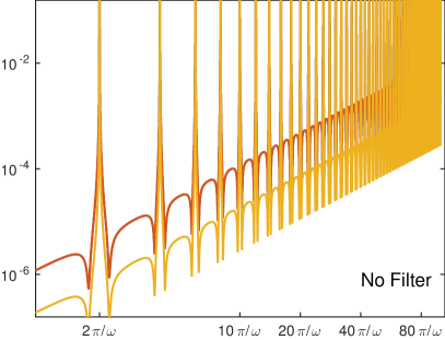
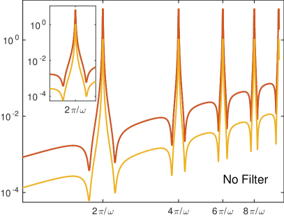
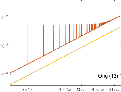
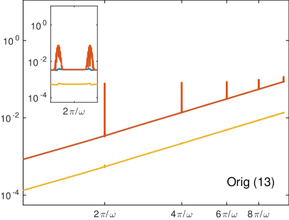
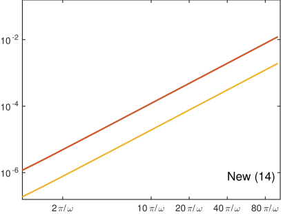
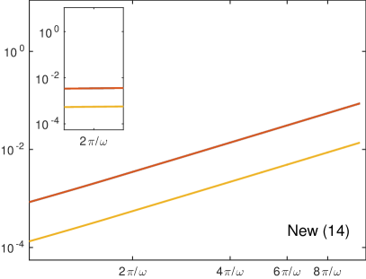
Figure 2: Euclidean norm of the absolute error of $\mathbf{e}$, $\mathbf{p}$ and $\mathbf{b}$ at $T=20$ versus step size for the numerical solution (4) measured against the spatially discrete reference solution of (2). Left: $\omega=8\cdot 10^{4}$; Right: $\omega=3\cdot 10^{3}$; Top: No filter; Middle: Filter of TuePLH10 ; Bottom: New filter choice (14).

8.2 Klein-Gordon type equation – two step method

We consider a one-dimensional Klein-Gordon type equation for one component of the electric field with periodic boundary conditions on the interval $[-10,14]$, where the plasma occupies the region $(10,11)$. This equation is obtained by eliminating $\mathbf{b}$ and $\mathbf{p}$ from (1). Discretization in space is by symmetric second order finite differences on the equidistant grid $x$ with grid points $x_{j}=-10+jh$, $j=1,\dots,N$, with $N=240$ and spacing $h=24/N$. The initial value $\mathbf{e}_{0}$ is given by (3) ($\bar{x}=0$, $\sigma_{0}=10$) evaluated on the grid and initial velocity by $(\dot{\mathbf{e}}_{0})_{j}=((\frac{2\pi}{\sigma_{0}})^{2}x_{j}\cos(2\pi x_{j})+2\pi\sin(2\pi x_{j}))\mathrm{e}^{-\frac{2\pi^{2}}{\sigma_{0}^{2}}x_{j}^{2}}$. That is we solve for $\mathbf{e}(t)$

$$\partial_{tt}\mathbf{e}(t) =\mathbf{G}\mathbf{e}(t)-\mathbf{\Omega}\mathbf{e}(t)\mbox{ for }t\in[0,3]$$ (51)

$$\mathbf{e}(0) =\mathbf{e}_{0},\quad\partial_{t}\mathbf{e}(0)=\dot{\mathbf{e}}_{0}$$

with, using Matlab notation, matrices $\mathbf{G}=\mathrm{spdiags}([e,-2*e,e],-1:1,N,N)/h^{2};$ $\mathbf{G}(1,N)=1/h^{2};$ $\mathbf{G}(N,1)=1/h^{2};$ for a vector $e$ with all ones and $f=0*x;$ $f(x<11\ \&\ x>10)=1;$ $\mathbf{\Omega}=\mathrm{diag}(\omega*f)$. with $\omega=9\cdot 10^{3}$.

We have implemented the two step method from (HaiLW06, , XIII.2.2) with even real-values filter functions $\psi$ and $\phi$, with $\psi(0)=\phi(0)=1$.

$$\mathrm{(A)} \ \psi(z) =\operatorname{sinc}^{2}(\tfrac{1}{2}z) \phi(z) =1$$ Gautschi Gautschi61

$$\mathrm{(B)} \ \psi(z) =\operatorname{sinc}(z) \phi(z) =1$$ Deuflhard Deuflhard79

$$\mathrm{(C)} \ \psi(z) =\operatorname{sinc}(\tfrac{1}{2}z)\phi(z) \phi(z) =\operatorname{sinc}(z)$$ Garcia-Archila et al. Garcia-Archilla1998

$$\mathrm{(D)} \ \psi(z) =\operatorname{sinc}^{2}(\tfrac{1}{2}z) \phi(z) \mbox{ from }\eqref{eq:phiHocL}\mbox{ below }$$ Hochbruck, Lubich HocL99

$$\mathrm{(E)} \ \psi(z) =\operatorname{sinc}^{2}(z) \phi(z) =1$$ Hairer, Lubich Hairer2001

$$\mathrm{(F)} \ \psi(z) =\eta(z)\operatorname{sinc}(z)^{2} \phi(z) =\operatorname{sinc}(\tfrac{1}{2}z) \eqref{eq:filterChoiceNew}$$

$$\mathrm{(G)} \ \psi(z) =\eta(z)\operatorname{sinc}(z) \phi(z) =\operatorname{sinc}(\tfrac{1}{2}z) \eqref{eq:filterChoiceJalo}~{}\mbox{ Liljo et al. \cite[cite]{\@@bibref{Authors Phrase1YearPhrase2}{TuePLH10}{\@@citephrase{(}}{\@@citephrase{)}}}}$$

$$\mathrm{(H)} \ \psi(z) =\operatorname{sinc}(\tfrac{1}{2}z) \phi(z) =\operatorname{sinc}(z)$$

$$\mathrm{(I)} \ \psi(z) =\operatorname{sinc}(z) \phi(z) =\operatorname{sinc}(\tfrac{1}{2}z),$$

where

$$\phi(z)=\operatorname{sinc}(z)(1+\tfrac{1}{3}\sin^{2}(\tfrac{1}{2}z))$$ (52)

in method (D). The alphabetic labels for methods (A) - (E) follow the convention of HaiLW06 . Method (F) corresponds to our choice, (14), with $\eta(z):=\tfrac{1}{2}(1+\cos(z))$ coming for free from the triple splitting. Method (G) corresponds to the choice (13) considered in TuePLH10 ; Lil10 .

Figure 3 shows the norm of the absolute error in euclidean norm versus the step size. For this linear test problem method (E) shows the same behavior as (A), the behavior of (D) is similar to (C) and (H) is similar (I), therefore results for (E), (D) and (H) are not displayed. The inset is a zoom to step sizes around $2\pi/\omega$ showing the error for $\tau\in[(2\pi-5\cdot 10^{-3})/\omega,(2\pi+5\cdot 10^{-3})/\omega]$. For this linear test problem one observes second order convergence as soon as there is a double zero of $\psi$ at even multiples of $2\pi$. The condition on $\phi$ seems to be less important. However comparing (I) and the method (B) it is observed that the resonance peak is much sharper for (I), reflecting the influence of $\phi$ in this test problem. Though the filter functions of methods (G), (H) and (I) satisfy the assumptions for first order convergence uniformly in $h\omega$ as predicted by (HaiLW06, , Theorem XIII.4.1), c.f. Remark 2, sharp resonance peaks are observed. Currently we suspect a mistake in the proof of the Theorem XIII.4.1 there.

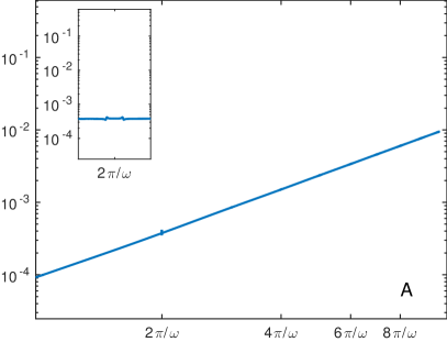
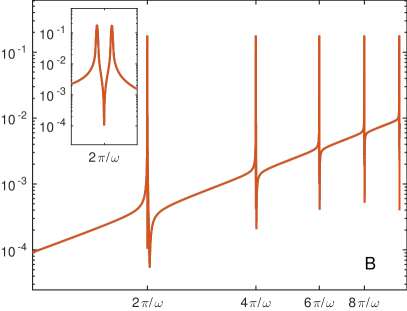
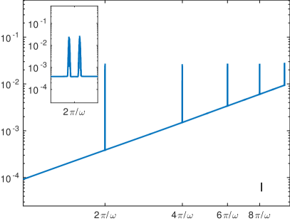
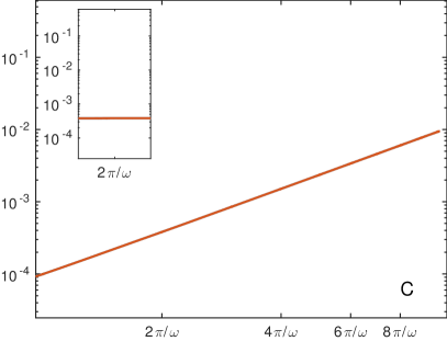
Figure 3: Euclidean norm of the absolute error at $T=3$ versus step size for the Klein-Gordon type equation (51). Results are shown for filter choices (A), (B), (C), (G), (I) and (F). The inset shows a zoom to step-sizes in the interval $[(2\pi-5\cdot 10^{-3})/\omega,(2\pi+5\cdot 10^{-3})/\omega]$.

References

- [1] Al-Mohy A.W. and Higham N. J. Computing the action of the matrix exponential, with an application to exponential integrators. SIAM Journal on Scientific Computing, 33(2):488–511, 2011.
- [2] S. Buchholz and M. Hochbruck. Error analysis of hybrid particle-in-cell (PIC) methods for oscillatory Maxwell-like equations. Book of Abstracts, 12th Int. Conf. on math. and numer. aspects of wave propagation (WAVES 2015, Karlsruhe, KIT, Germany), 2015.
- [3] P. Deuflhard. A study of extrapolation methods based on multistep schemes without parasitic solutions. Zeitschrift für angewandte Mathematik und Physik ZAMP, 30(2):177–189, 1979.
- [4] B. Garcia-Archilla, J.M. Sanz-Serna, and R.D. Skeel. Long-time-step methods for oscillatory differential equations. SIAM Journal on Scientific Computing, 20(3):930–963, 1998.
- [5] W. Gautschi. Numerical integration of ordinary differential equations based on trigonometric polynomials. Numerische Mathematik, 3(1):381–397, 1961.
- [6] V. Grimm and M. Hochbruck. Error analysis of exponential integrators for oscillatory second-order differential equations. Journal of Physics A: Mathematical and General, 39:5495–5507, 2006.
- [7] E. Hairer and Ch. Lubich. Long-time energy conservation of numerical methods for oscillatory differential equations. SIAM Journal on Numerical Analysis, 38(2):414–441, 2001.
- [8] E. Hairer, Ch. Lubich, and G. Wanner. Geometric numerical integration, volume 31 of Springer Series in Computational Mathematics. Springer-Verlag, Berlin, second edition, 2006. Structure-preserving algorithms for ordinary differential equations.
- [9] R. Hiptmair. Finite elements in computational electromagnetism. Acta Numer., 11:237–339, 2002.
- [10] R. Hiptmair, P. R. Kotiuga, and S. Tordeux. Self-adjoint curl operators. Annali di Matematica Pura ed Applicata, 191(3):431–457, 2012.
- [11] M. Hochbruck and Ch. Lubich. A Gautschi-type method for oscillatory second-order differential equations. Numerische Mathematik, 83(3):403–426, 1999.
- [12] G. Jansing. Exponentielle Integratoren – Zeitintegrationsverfahren für Maxwell-Gleichungen und parabolische Systeme. Dissertation, Heinrich-Heine Universität Düsseldorf, 2015.
- [13] J. Liljo. Hybride Verfahren zur Simulation der Wechselwirkung relativistischer Kurzpuls-Laser mit hochdichten Plasmen. Dissertation, Heinrich-Heine Universität Düsseldorf, 2010.
- [14] T. Tückmantel. Hybrid particle-in-cell simulations of relativistic plasmas. Dissertation, Heinrich-Heine Universität Düsseldorf, 2013.
- [15] T. Tückmantel, A. Pukhov, J. Liljo, and M. Hochbruck. Three-dimensional relativistic particle-in-cell hybrid code based on an exponential integrator. IEEE Transactions on Plasma Science, 38(9):2383–2389, 2010.