Multi-Dimensional Pass-Through and Welfare Measures under Imperfect Competition

Abstract

This paper provides a comprehensive analysis of welfare measures when oligopolistic firms face multiple policy interventions and external changes under general forms of market demands, production costs, and imperfect competition. We present our results in terms of two welfare measures, namely, marginal cost of public funds and incidence, in relation to multi-dimensional pass-through. Our arguments are best understood with two-dimensional taxation where homogeneous firms face unit and ad valorem taxes. The first part of the paper studies this leading case. We show, e.g., that there exists a simple and empirically relevant set of sufficient statistics for the marginal cost of public funds, namely unit tax and ad valorem pass-through and industry demand elasticity. We then specialize our general setting to the case of price or quantity competition and show how the marginal cost of public funds and the pass-through are expressed using elasticities and curvatures of regular and inverse demands. Based on the results of the leading case, the second part of the paper presents a generalization with the tax revenue function specified as a general function parameterized by a vector of multi-dimensional tax parameters. We then argue that our results are carried over to the case of heterogeneous firms and other extensions.

1 Introduction

In many economic situations, it is important to understand the impact of changes in government policies, market conditions, or production technology. Both the impact on the economic equilibrium and the associated change in the welfare of individual economic agents are of interest to the policymaker. A convenient framework for studying these questions is laid out in Weyl and Fabinger (2013) for the case of constant changes in marginal cost such as a unit tax. In this paper, we provide a substantial generalization of this framework under general forms of market demands, production costs, and imperfect competition. We allow not only for changes in costs proportional to the value of the goods such as an ad-valorem tax but also for much more general interventions such as different kinds of market regulation. In addition, we provide a new perspective on the case of heterogeneous firms.

The range of possibilities for governments’ intervention is much richer than just specific and ad-valorem taxes, on which the existing literature has focused (see Section 2), especially if we consider regulations of various kinds. Governments often intervene in the marketplace by restricting sales. Examples include restrictions of sales on Sundays and holidays in many European countries, or restrictions of sales of alcohol, both in terms of time of sales and in terms of locations where sales are allowed. Governments also often regulate the labor market. Examples include restrictions on the number of working hours or stipulation of a minimum wage. Besides these, governments also impose reporting requirements that influence the degree to which non-compliant firms misreport their marketplace data to minimize their tax bill.

Given that there are many possible interventions, it is convenient to summarize the interventions of interest in a (multi-dimensional) vector. The impact of infinitesimal changes in these interventions on prices then corresponds to a vector (or more generally a matrix), which may be termed multi-dimensional pass-through. The relative size of its components then provides insight into the relationship between the impact of individual interventions, for example, the impact of specific vs.  ad-valorem taxes. We show that the multi-dimensional pass-through is an important determinant of the welfare effects of various kinds of interventions.

Our arguments are best understood with two-dimensional taxation where homogeneous firms face unit and ad valorem taxes. Therefore, in the first part of the paper (Sections 2 and 3), we derive succinct formulas that relate the marginal cost of public funds to pass-through of these taxes. We also establish a relationship that connects pass-through of unit taxes and pass-through of ad-valorem taxes in the same market. Furthermore, we derive convenient expressions for values of unit and ad valorem pass-through that are valid under a “general” type competition and have not appeared in the previous literature. In addition, we show how the marginal cost of public funds and pass-through are expressed in terms of elasticities and curvatures of demand and inverse demand when the setting is specialized to price (differentiated Bertrand) or quantity (pure or differentiated Cournot) competition. We also provide numerical examples. Our results also apply without a change to symmetric oligopoly with multi-product firms. Throughout the analysis, we allow for non-zero levels of unit and ad valorem taxes. However, we also discuss some additional simplifications that appear when instead the initial level of taxes is zero.

Inspired by the results of this setting of two-dimensional taxation, the second part of the paper generalizes our model in two directions (Sections 4, 5, and 6). First, we allow for interventions that are more general than just specific and ad valorem taxes. Second, we introduce firm heterogeneity. We find that these more general relationships have a form that still relatively simple and succinct. This substantially expands the applicability of our results.

From both theoretical and empirical standpoints, it is desirable to be able to understand the welfare properties of oligopolistic markets with a fairly general type of competition. In real-world situations, firms’ behavior may not simply be categorized into either the idealized price competition or the idealized quantity competition. Price competition does not allow for any friction in scaling production levels up or down, yet in reality there tend to be substantial frictions, such as those related to financial constraints or the labor market. Quantity competition implies that the firm will not be able to increase production levels when its competitor suddenly decides to increase prices. In reality, such adjustment is probably feasible, since capacity utilization is typically less than complete, and even if the firm is operating at full capacity, boosting production levels is possible by overtime work or by hiring temporary workers. Moreover, firms may behave, to some extent, in a collusive way. Although the realities of competition by firms may be complicated, it is possible to capture their essence by working with a “general” type of competition, using the conduct index.

Besides working with a more general type of competition, it is also useful to relax the assumption of constant marginal costs that often appears in the literature. Production technologies often have a non-trivial structure, and so does the internal organization of the firm. For example, if a firm decides to operate at a larger scale, it may take advantage of technological and logistical economies of scale, but at the same time, it may face more severe principal-agent problems as top managers have to delegate responsibilities to lower-level managers. The interplay between these forces can lead to a non-trivial dependence of the marginal cost of production on the scale of the operation. A notable benefit from our general framework is that one does not necessarily have to assume constant marginal cost in conducting welfare assessment in a precise manner.

In this spirit, the aim of Weyl and Fabinger’s (2013) study is to analyze imperfect competition in a way that does not rely on limiting functional form assumptions. It is followed by Fabinger and Weyl (2018), who propose using further flexible functional forms to make economic models or their parts solvable in closed form. The present paper goes in a different direction: we focus on more general market interventions and exogenous market changes without requiring that the models or their parts be solved in closed form. As mentioned above, ad valorem taxes are not studied in Weyl and Fabinger (2013). In this paper, we provide a more general framework that allows not only for ad valorem taxes but for other interventions in a general manner.

The rest of the paper mainly consists of two parts: the first part focuses on the canonical situation of two-dimensional taxation where symmetric firms face unit and ad valorem taxes, and the second part extends these results to a more general framework of multiple government interventions and external changes, allowing firm heterogeneity. First, in the next section, we set up a framework of two-dimensional taxation under imperfect competition and provide general formulas for marginal cost of public funds and incidence in relation to unit tax and ad valorem tax pass-throughs and industry demand elasticity. In Section 3, we specialize this setting to the case of price or quantity competition. Then, in the second part of the paper, Section 4 generalizes the results from unit and ad valorem taxation to much more flexible taxation parameterized by $d$ different tax parameters and discusses the implications of these general results. We also discuss other types of government/exogenous interventions that are suitable for our framework. Then, in Section 5 we generalize our formulas to include heterogeneous firms. Finally, Section 6 generalizes our previous results to include changes in both production costs and taxes. Section 7 concludes the paper.

2 Taxation and Welfare in Symmetric Oligopoly

We begin with a canonical setting where firms face two types of taxation: unit and ad valorem taxes. This issue has been in the central part of the existing literature on government interventions. The welfare cost of taxation has been extensively studied at least since Pigou (1928). The majority of the studies simply assume perfect competition (with zero initial taxes). As is widely known, under perfect competition, unit tax and ad valorem tax are equivalent, and whether consumers or producers bear more is determined by the relative elasticities of demand and supply (Weyl and Fabinger, 2013, p. 534). The initial attempt to relax the assumption of perfect competition started with an analysis of homogeneous-product oligopoly under quantity competition, i.e., Cournot oligopoly. Notably, Delipalla and Keen (1992), Skeath and Trandel (1994), and Hamilton (1999) compare ad valorem and unit taxes in such a setting. Then, Anderson, de Palma, and Kreider (2001a) extend these results to the case of differentiated oligopoly under price competition. In particular, Anderson, de Palma, and Kreider (2001a) find that whether the after-tax price for firms and their profits rise by a change in ad valorem tax depends importantly on the ratio of the curvature of the firm’s own demand to the elasticity of the market demand.

In this section, we extend Anderson, de Palma, and Kreider’s (2001a) setting and results in a number of important directions. First, we consider a “general” mode of competition, captured by the conduct index, including both quantity and price competition. Second, we provide a complete characterization of tax burdens that enables one to quantitatively compare consumers’ burden with producers’ burden, whereas Anderson, de Palma, and Kreider’s (2001a) focus only on the effective prices for consumers and producers’ profits. Third, while Anderson, de Palma, and Kreider’s (2001a) assume constant marginal cost, we allow non-constant marginal cost and show how this generalization makes a difference in our general formulas. Fourth, we further generalize the initial tax level. When they analyze the effects of a unit tax, Anderson, de Palma, and Kreider (2001a) assume that ad valorem tax is zero, and vice versa. In contrast, we allow non-zero initial taxes in both dimensions. Finally, and importantly, we generalize these results to the case of a very general type of taxation, as well as to production cost changes. This opens up the possibility to study a wider range of interventions/taxes and to derive convenient sufficient statistics for characteristics, including welfare characteristics, of the markets of interest.

2.1 Setup

Below, we study oligopolistic markets with $n$ symmetric firms and a general (first-order) mode of competition and the resulting symmetric equilibria. Our discussion applies to single-product firms as well as to multi-product firms if intra-firm symmetry conditions are satisfied, as discussed in Appendix A.1.12. For simplicity of exposition, we use terminology corresponding to single-product firms here, and later we discuss how to interpret the results in the case of multi-product firms.

Formally, the demand for firm $j$’s product $q_{j}=q_{j}(p_{1},...,p_{n})\equiv q_{j}\left(\mathbf{p}\right)$ depends on the vector of prices $\mathbf{p}\equiv\left(p_{1},...,p_{n}\right)$ charged by the individual firms. The demand system is symmetric and the cost function $c(q_{j})$ is the same for all firms. We assume that $q_{j}(\cdot)$ and $c(\cdot)$ are twice differentiable and conditions for the uniqueness of equilibrium and the associated second-order conditions are satisfied. We denote by $q(p)$ the per-firm industry demand corresponding to symmetric prices: $q(p)\equiv q_{j}(p,...,p)$. The elasticity of this function, defined as $\epsilon(p)\equiv-pq^{\prime}(p)/q(p)>0$ and referred to as the price elasticity of industry demand, should not be confused with the elasticity of the residual demand that any of the firms faces. We also use the notation $\eta(q)=1/\epsilon\left(p\right)|_{q\left(p\right)=q}$ for the reciprocal of this elasticity as a function of $q$. For the corresponding functional values, when we do not need to specify explicitly their dependence on either $q$ or $p$, we use $\eta$ interchangeably with $1/\epsilon$.

As mentioned above, we introduce two types of taxation: a unit tax $t$ and an ad valorem tax $v$, with firm $j$’s profit being $\pi_{j}=(1-v)p_{j}(q_{j})q_{j}-tq_{j}-c(q_{j})$. At symmetric quantities the government tax revenue per firm is $R\left(q\right)\equiv tq+vp\left(q\right)q$, and we denote by $\tau\left(q\right)$ the fraction of firm’s pre-tax revenue that is collected by the government in the form of taxes: $\tau\left(q\right)\equiv R\left(q\right)/pq=v+t/p\left(q\right)$. We now introduce the conduct index $\theta(q)$, which measures the industry’s competitiveness (a lower $\theta$ corresponds to a fiercer level of competition). Here, it is determined independently of the cost side but potentially can change for different values of the industry’s output, $q$. Then, the symmetric equilibrium condition is written as

$$\frac{1}{\eta\left(q\right)p\left(q\right)}\left(p\left(q\right)-\dfrac{t+mc\left(q\right)}{1-v}\right)=\theta(q)\text{,}$$ (1)

where $mc(q)\equiv c^{\prime}(q)$ is the marginal cost of production. We denote by $\theta$ the functional value of $\theta(q)$ at the equilibrium quantity. This is also understood as the elasticity-adjusted Lerner index: the markup rate $[p-(t+mc)/(1-v)]/p$ should be adjusted by the industry-wide elasticity to reflect the competitiveness in the industry, where $(t+mc)/(1-v)$ is interpreted as the effective marginal cost. We emphasize here that once the conduct index is introduced, one is able to describe oligopoly in a synthetic manner, without specifying whether it is price or quantity setting, or whether it exhibits strategic substitutability or complementarity.

2.2 The marginal cost of public funds and pass-through

The marginal cost of public funds, i.e., the marginal social welfare loss associated with raising additional tax revenue, is a crucial characteristic that a policymaker needs to take into account when designing an optimal system of taxes. In the special case of linear demand and constant marginal cost, Häckner and Herzing (2016, p. 147) explain that as long as the initial level of taxes is zero, the marginal cost of public funds for unit taxation equals $MC_{t}=\theta\rho_{t}$, where $\rho_{t}$ is the unit-tax pass-through rate (the marginal effect of unit taxes on prices), and $\theta$ is the conduct index. For ad valorem taxes, Häckner and Herzing (2016) provide a similar formula. They argue, however, that if we let the initial level of taxes be non-zero, those formulas are no longer valid. For this reason, they are forced to analyze the magnitude of the marginal cost of public funds on a case-by-case basis using explicit solutions to specific models.

This situation represents a puzzle. If there are simple formulas for the marginal cost of public funds that were valid at zero taxes, is there no compact generalization of these expressions in the case of non-zero taxes? If there is no such generalization, that would be an obstacle to empirical work, since we would have to make additional modeling assumptions before obtaining empirical estimates of the marginal cost of public funds. Our paper provides a solution to this problem. In particular, Proposition 1 below presents formulas for the marginal cost of public funds that are valid even when the initial level of (both ad valorem and unit) taxes is non-zero. They are a bit longer than $MC_{t}=\theta\rho_{t}$, but still very manageable. They also represent a starting point for the topics discussed in the rest of the paper. These results with a non-zero initial taxes being allowed, which are differentiated from Weyl and Fabinger (2013) and Häckner and Herzing (2016), should be useful if one needs to evaluate the marginal cost of taxation when some tax has been already implemented.

The marginal welfare cost $MC_{t}$ or $MC_{v}$ of raising government revenue by the unit tax $t$ or the ad valorem tax $v$, i.e. the marginal cost of public funds associated with such a tax, is defined as

$$MC_{t}\equiv-\left(\frac{\partial R}{\partial t}\right)^{-1}\frac{\partial W}{\partial t},\qquad MC_{v}\equiv-\left(\frac{\partial R}{\partial v}\right)^{-1}\frac{\partial W}{\partial v},$$

where $W$ is the social welfare per firm, which includes consumer surplus, producer surplus, and government tax revenue. We define the unit tax pass-through rate $\rho_{t}$ and the ad valorem tax pass-through semi-elasticity $\rho_{v}$ as:

$$\rho_{t}=\frac{\partial p}{\partial t},\qquad\rho_{v}=\frac{1}{p}\ \frac{\partial p}{\partial v}.$$

Consider an infinitesimal change in the unit tax, with the initial tax level $(t,v)$. As mentioned in the introduction, in the special case of zero initial taxes, linear demand, and constant marginal cost, Häckner and Herzing (2016, p. 147) show that $MC_{t}=\theta\rho_{t}$ and $MC_{v}=\theta\rho_{v}$, noting that at non-zero initial taxes the formula no longer applies. In the absence of such formula, they were forced to study the marginal cost of public funds on a case-by-case basis, for different specifications of demand and cost.

Intuitively, there are at least two reasons why $\theta\rho_{t}$ fails to be an accurate measure of the marginal cost of public funds when a unit tax is raised. First, the expression is simply proportional to $\theta$, but when $v$ is large, the firms sell at prices that are too high from the social perspective not mainly because of a lack of competitiveness, but primarily because the tax effectively raises their perceived cost. When $v$ is large, we would expect the marginal cost of public funds to be less sensitive to $\theta$, for a given value of $\rho_{t}$. Second, the expression $\theta\rho_{t}$ does not explicitly feature the level of the unit tax $t$. However, a situation where $t$ is large and $mc$ small is very different from a situation where $t$ is small and $mc$ large, even if the equilibrium prices and quantities are the same. In the former case, raising additional tax revenue is quite harmful, since firms’ production cuts will not substantially decrease the total technological (i.e., pre-tax) cost of production. In the latter case, raising additional tax revenue is less harmful since it leads to reduced total technological cost. Based on this intuition, we would expect the marginal cost of public funds to be an increasing function of $t$.

Thus, we are led to find a generalization of the formula $MC_{t}=\theta\rho_{t}$ and $MC_{v}=\theta\rho_{v}$ that would be applicable even at non-zero initial taxes. It turns out that it is possible to identify a formula with precisely these properties, as the following proposition shows.

Proposition 1.

Marginal cost and total of public funds for unit and ad valorem taxations. Under symmetric oligopoly with a possibly non-constant marginal cost, the marginal cost of public funds associated with a unit tax may be expressed as

$$MC_{t}=\frac{(1-v)\thinspace\theta+\epsilon\thinspace\tau}{\frac{1}{\rho_{t}}+v-\epsilon\thinspace\tau},$$

and the marginal cost of public funds associated with an ad valorem tax may be expressed as

$$MC_{v}=\frac{(1-v)\thinspace\theta+\epsilon\tau}{\frac{1}{\rho_{v}}+v-\epsilon\tau}.$$

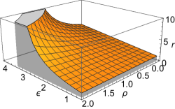
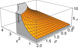
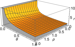
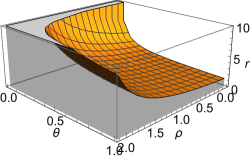
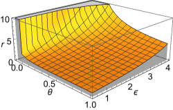
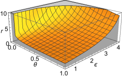
Figure I: The ratio of the actual marginal cost of public funds $MC$ and the naive expression $\theta\rho$ discussed just before Proposition 1, plotted as a function of combinations of the conduct index $\theta$, the pass-through $\rho$, and the industry demand elasticity $\epsilon$. The figures on the left correspond to infinitesimal changes in unit taxation: $\rho$ stands for $\rho_{t}$ and $MC$ stands for $MC_{t}$. The numerical values were chosen to be $t=0,\ v=0.2,\ \tau=0.2$. The figures on the right correspond to infinitesimal changes in ad valorem taxation: $\rho$ stands for $\rho_{v}$ and $MC$ stands for $MC_{v}$. The numerical values were chosen to be $t/p=0.2,\ v=0,\ \tau=0.2$. The top figures correspond to $\theta=0.3$, the middle figures correspond to $\epsilon=2$, and the bottom figures correspond to $\rho=1$.

The proposition is proven in Appendix A.1.1 and the intuition behind it is discussed in detail in Appendix A.1.2. Here in the main text we just include Figure I, which documents that these expressions for the marginal cost of public funds $MC_{t}$ and $MC_{v}$ evaluated at realistic values of taxes and other economic variables are very different from the values of the expressions $\theta\rho_{t}$ and $\theta\rho_{v}$ (discussed above) that would be equal to $MC_{t}$ and $MC_{v}$ if taxes were zero.

2.3 Incidence and pass-through

We define the incidence $I_{t}$ of unit taxation as the ratio of changes $dCS$ in (per-firm) consumer surplus and changes $dPS$ in (per-firm) producer surplus induced by an infinitesimal increase $dt$ in the unit tax $t$. The incidence $I_{v}$ of ad valorem taxation is defined analogously. We obtain the following succinct results for the incidence of taxation at non-zero unit and ad valorem taxes.

Proposition 2.

Incidence of taxation. Under symmetric oligopoly with a general type of competition and with a possibly non-constant marginal cost, the incidence of unit taxes $I_{t}$ and of ad valorem taxes $I_{v}$ is given by

$$\frac{1}{I_{t}}=\frac{1}{\rho_{t}}-\left(1-v\right)\left(1-\theta\right),\qquad\frac{1}{I_{v}}=\frac{1}{\rho_{v}}-\left(1-v\right)\left(1-\theta\right).$$

The proposition is proven in Appendix A.1.3, and we discuss it in detail in Appendix A.1.4. Note that in the case of zero ad valorem tax, the expression for $I_{t}$ reduces to Weyl and Fabinger’s (2013, p. 548) Principle of Incidence 3. Next we show how $\rho_{t}$ and $\rho_{v}$ are related in the following proposition.

Proposition 3.

Relationship between pass-through of ad valorem and unit taxes. Under symmetric oligopoly with a possibly non-constant marginal cost, the pass-through semi-elasticity $\rho_{v}$ of an ad valorem tax may be expressed in terms of the unit tax pass-through rate $\rho_{t}$, the conduct index $\theta$, and the industry demand elasticity $\epsilon$ as

$$\rho_{v}=\left(1-\frac{\theta}{\epsilon}\right)\ \rho_{t}.$$ (2)

The proposition is proven Appendix A.1.5, and Appendix A.1.6 provides a detailed discussion. Combined with Proposition 1, it is consistent with the well-known result that unit tax and ad valorem tax are equivalent in the welfare effects under perfect competition: if $\theta=0$, then $\rho_{t}=\rho_{v}$. Under imperfect competition, $\rho_{t}>\rho_{v}$, and $MC_{t}>MC_{v}$. This provides another look of Anderson, de Palma, and Kreider’s (2001b) result that unit taxes are welfare-inferior to ad valorem taxes.

By combining Propositions 1 and 3, we find that $MC_{t}$ and $MC_{v}$ can be expressed without the degree of competitiveness $\theta$.

Proposition 4.

Sufficient statistics for marginal costs of public funds. Under symmetric oligopoly with a possibly non-constant marginal cost, the unit pass-through rate $\rho_{t}$, the ad valorem pass-through semi-elasticity $\rho_{v}$, and the elasticity $\epsilon$ of industry demand (together with the tax rates and the fraction $\tau$ of the firm’s pre-tax revenue collected by the government in the form of taxes) serve as sufficient statistics for the marginal cost of public funds both with respect to unit taxes and ad valorem taxes. In particular:

$$MC_{t}=\frac{(1-v+\tau)\rho_{t}-(1-v)\rho_{v}}{1+(v-\epsilon\tau)\rho_{t}}\ \epsilon,\qquad MC_{v}=\frac{\left(1-v+\tau\right)\rho_{t}-(1-v)\rho_{v}}{1+\left(v-\epsilon\tau\right)\rho_{v}}\ \frac{\rho_{v}}{\rho_{t}}\epsilon.$$

The proof is simple: Proposition 3 allows us to express the conduct index $\theta$ as $\theta=(1-\rho_{v}/\rho_{t})\epsilon$. Substituting this into the relationships in Proposition 1 then gives the desired result. For a detailed discussion of related intuition, see Appendix A.1.7.

As the last result presented in this section, the following proposition shows how the two forms of pass-through are characterized.

Proposition 5.

Pass-through under symmetric oligopoly. Under symmetric oligopoly with a general (first-order) mode of competition and with a possibly non-constant marginal cost:

$$\rho_{t}=\frac{1}{1-v}\ \frac{1}{\left[1+\frac{1-\tau}{1-v}\epsilon\chi\right]-\left(\eta+\chi\right)\theta+\epsilon q\left(\theta\eta\right)^{\prime}},$$

where the derivative is taken with respect to $q$ and $\chi\equiv mc^{\prime}q/mc$ is the elasticity of the marginal cost with respect to quantity. Further,

$$\rho_{v}=\frac{\epsilon-\theta}{\left(1-v\right)\epsilon}\ \frac{1}{\left[1+\frac{1-\tau}{1-v}\epsilon\chi\right]-\left(\eta+\chi\right)\theta+\epsilon q\left(\theta\eta\right)^{\prime}}.$$

The proof and a related discussion are in Appendix A.1.8. Further, we discuss a relationship with Weyl and Fabinger (2013) in Appendix A.1.9, provide a comparison of perfect and oligopolistic competition in Appendix A.1.10, and show the applicability of these results to exchange rate changes in Appendix A.1.11.

2.4 Global changes in surplus measures

So far, we have discussed local, i.e. infinitesimal, changes in surplus measures ($CS$, $PS$, $R$, $W$). For larger changes in some tax $T$, it is desirable to have an understanding of global changes in surplus measures. Consider surplus measures $A$ and $B$. Their finite changes $\Delta A=\int_{T_{1}}^{T_{2}}\frac{dA\left(T\right)}{dT}dT$ and $\Delta B=\int_{T_{1}}^{T_{2}}\frac{dB\left(T\right)}{dT}dT$ induced by a tax change from $T=T_{1}$ to $T=T_{2}$ are related to their incidence ratios $\Theta{}_{AB}\equiv\frac{dA\left(T\right)}{dT}/\frac{dB\left(T\right)}{dT}$. In particular, $\Delta A/\Delta B$ is a weighted average of $\Theta{}_{AB}$ over the interval $\left(T_{1},T_{2}\right)$:

$$\frac{\Delta A}{\Delta B}=\int_{T\in\left(T_{1},T_{2}\right)}\!\!\!\Theta{}_{AB}\,dw_{B}^{\left(T_{1},T_{2}\right)}\!\left(T\right),$$

where $dw_{B}^{\left(T_{1},T_{2}\right)}\!\left(T\right)\equiv\frac{dB\left(T\right)}{dT}dT/\int_{T_{1}}^{T_{2}}\frac{dB\left(T^{\prime}\right)}{dT^{\prime}}dT^{\prime}$ is a weight normalized to one on the corresponding interval: $\int_{T_{1}}^{T_{2}}dw_{B}^{\left(T_{1},T_{2}\right)}\!\left(T\right)=1$. The weight is positive as long as $\frac{dB\left(T\right)}{dT}$ has the same sign as $\int_{T_{1}}^{T_{2}}\frac{dB\left(T\right)}{dT}dT$, which is typically satisfied in useful applications. In many useful cases $A$ and $B$ are zero at infinite $T$. Then

$$\frac{A\left(T_{1}\right)}{B\left(T_{1}\right)}=\int_{T\in\left(T_{1},\infty\right)}\!\!\!\Theta{}_{AB}\,dw_{B}^{\left(T_{1},\infty\right)}\!\left(T\right).$$

For example,

$$\frac{CS\left(T_{1}\right)}{PS\left(T_{1}\right)}=\int_{T\in\left(T_{1},\infty\right)}\!\!\!I_{T}\,dw_{PS}^{\left(T_{1},\infty\right)}\!\left(T\right),\qquad\frac{W\left(T_{1}\right)}{R\left(T_{1}\right)}=\int_{T\in\left(T_{1},\infty\right)}\!\!\!MC_{T}\,dw_{R}^{\left(T_{1},\infty\right)}\!\left(T\right).$$

In the case of a per-unit tax, we obtain

$$\frac{CS\left(t_{1}\right)}{PS\left(t_{1}\right)}=\frac{\int_{t_{1}}^{\infty}I{}_{T}\,q\,dt}{\int_{t_{1}}^{\infty}q\,dt}.$$

3 Taxation and Welfare under Specific Types of Competition

In this section, we show that for price competition and quantity competition in differentiated oligopoly, our general expressions of the marginal cost of public funds and pass-through lead to expressions in terms of demand primitives such as the elasticities and the curvatures, and the marginal cost elasticity $\chi$ defined above. Throughout this section, we assume that firms’ conduct is simply described by one-shot Nash behavior, without any other further possibilities such as tacit collusion. As seen below, this assumption enables one to express the conduct index in terms of demand and inverse demand elasticities, using Equation (1) directly (see Subsection 3.2). We also provide parametric examples for these results.

3.1 Elasticities and curvatures of the demand system

Direct demand. Following Holmes (1989, p. 245), we define the own price elasticity $\epsilon_{F}(p)$ and the cross price elasticity $\epsilon_{C}(p)$ of the firm’s direct demand by

$$\epsilon_{F}(p)\equiv-\frac{p}{q\left(p\right)}\ \frac{\partial q_{j}(\mathbf{p})}{\partial p_{j}}|_{\mathbf{p}=\left(p,...,p\right)},\qquad\epsilon_{C}(p)\equiv\frac{(n-1)p}{q\left(p\right)}\ \frac{\partial q_{j^{\prime}}(\mathbf{p})}{\partial p_{j}}|_{\mathbf{p}=\left(p,...,p\right)},$$

where $j$ and $j^{\prime}$ is an arbitrary pair of distinct indices. These are related to the industry demand elasticity $\epsilon(p)$ by $\epsilon_{F}=\epsilon+\epsilon_{C}$. Next, we define the curvature of the industry’s direct demand $\alpha(p)$, the own curvature $\alpha_{F}(p)$ of the firm’s direct demand and the cross curvature $\alpha_{C}(p)$ of the firm’s direct demand:

$$\alpha(p)\!\equiv\!\frac{-pq^{\prime\prime}(p)}{q^{\prime}(p)}\!,\alpha_{F}(p)\!\equiv\!-p\!\left(\!\frac{\partial q_{j}(\mathbf{p})}{\partial p_{j}}\!\right)^{\!\!\!-1}\!\!\frac{\partial^{2}\!q_{j}(\mathbf{p})}{\partial p_{j}^{2}}\!,\alpha_{C}(p)\!\equiv\!-\!\left(n\!-\!1\right)\!p\!\left(\!\frac{\partial q_{j}(\mathbf{p})}{\partial p_{j}}\!\right)^{\!\!\!-1}\!\!\frac{\partial^{2}\!q_{j}(\mathbf{p})}{\partial p_{j}\,\!\partial p_{j^{\prime}}},$$

where again the derivatives are evaluated at $\mathbf{p}=\left(p,...,p\right)$, and $j$ and $j^{\prime}$ is an arbitrary pair of distinct indices. These curvatures satisfy $\alpha=(\alpha_{F}+\alpha_{C})\epsilon_{F}/\epsilon$ and are related to the elasticity of $\epsilon_{F}(p)$ by $p\,\epsilon_{F}^{\prime}(p)/\epsilon_{F}(p)=1+\epsilon\left(p\right)-\alpha_{F}\left(p\right)-\alpha_{C}\left(p\right)$ (see Appendix A.2.1 for the derivation and a related discussion).

Inverse demand. We introduce analogous definitions for inverse demand. We define the own quantity elasticity $\eta_{F}(q)$ and the cross quantity elasticity $\eta_{C}(q)$ of the firm’s inverse demand as

$$\eta_{F}(q)\equiv-\frac{q}{p(q)}\ \frac{\partial p_{j}(\mathbf{q})}{\partial q_{j}}|_{\mathbf{q}=\left(q,...,q\right)},\qquad\eta_{C}(q)\equiv(n-1)\frac{q}{p(q)}\ \frac{\partial p_{j^{\prime}}(\mathbf{q})}{\partial q_{j}}|_{\mathbf{q}=\left(q,...,q\right)},$$

for arbitrary distinct $j$ and $j^{\prime}$. These satisfy $\eta_{F}=\eta+\eta_{C}$. We define the curvature of the industry’s inverse demand $\sigma(q)$, the own curvature $\sigma_{F}(q)$ of the firm’s inverse demand and the cross curvature $\sigma_{C}(q)$ of the firm’s inverse demand by:

$$\sigma(q)\!\equiv\!\frac{-qp^{\prime\prime}(q)}{p^{\prime}(q)}\!,\,\sigma_{F}(q)\!\equiv\!-q\!\left(\!\frac{\partial p_{j}(\mathbf{q})}{\partial q_{j}}\!\right)^{\!\!\!-1}\!\!\frac{\partial^{2}p_{j}(\mathbf{q})}{\partial q_{j}^{2}}\!,\,\sigma_{C}(q)\!\equiv\!-\!\left(n\!-\!1\right)\!q\!\left(\!\frac{\partial p_{j}(\mathbf{q})}{\partial q_{j}}\!\right)^{\!\!\!-1}\!\!\frac{\partial^{2}\!p_{j}(\mathbf{q})}{\partial q_{j}\!\,\partial q_{j^{\prime}}},$$

where again the derivatives are evaluated at $\mathbf{q}=\left(q,...,q\right)$ and the indices $j$ and $j^{\prime}$ are distinct. These curvatures represent an oligopoly counterpart of monopoly $\sigma(q)$ of Aguirre, Cowan, and Vickers (2010, p. 1603). They satisfy the relationship $\sigma=(\sigma_{F}+\sigma_{C})(\eta_{F}/\eta)$ and are related to the elasticity of $\eta_{F}(q)$ by $q\,\eta_{F}^{\prime}(q)/\eta_{F}(q)=1+\eta\left(q\right)-\sigma_{F}\left(q\right)-\sigma_{C}\left(q\right)$ (see Appendix A.2.2 for the derivation and a related discussion).

3.2 Expressions for conduct index and pass-through

In the case of price competition, the conduct index $\theta$ is $\theta=\epsilon/\epsilon_{F}=1/(\eta\epsilon_{F})$, which is verified by comparing the firm’s first-order condition with Equation (1). The marginal cost of public funds and the incidence are obtained by substituting these expressions into those of Propositions 1 and 2.

Proposition 6.

Pass-through under price competition. Under symmetric oligopoly with price competition and with a possibly non-constant marginal cost:

$$\rho_{t}=\frac{1}{1-v}\ \frac{1}{1+\frac{(1-\alpha/\epsilon_{F})\epsilon}{\epsilon_{F}}+\left(\frac{1-\tau}{1-v}-\frac{1}{\epsilon_{F}}\right)\epsilon\chi},$$

$$\rho_{v}=\frac{1}{1-v}\ \frac{1}{\frac{1}{1-1/\epsilon_{F}}+\frac{(1-\alpha/\epsilon_{F})\epsilon}{\epsilon_{F}-1}+\left(\frac{1-\tau}{1-v}\,\frac{\epsilon_{F}}{\epsilon_{F}-1}-\frac{1}{\epsilon_{F}-1}\right)\epsilon\,\chi}.$$

The proof is in Appendix A.2.3 and a detailed discussed in Appendix A.2.4.

Next, in the case of quantity competition, the conduct index $\theta$ is given by $\theta=\eta_{F}/\eta$, which is, again, verified by comparing the firm’s first-order condition with Equation (1). Again, the marginal cost of public funds and the incidence are obtained by substituting these expressions into those of Propositions 1 and 2. For the proof and a related discussion, see Appendix A.2.5 and A.2.6.

Proposition 7.

Pass-through under quantity competition. Under symmetric oligopoly with quantity competition and with a possibly non-constant marginal cost:

$$\rho_{t}\!=\!\frac{1}{1-v}\ \frac{1}{1+\frac{\eta_{F}}{\eta}-\sigma+\!\left(\frac{1-\tau}{1-v}-\eta_{F}\right)\frac{\chi}{\eta}},\qquad\rho_{v}\!=\!\frac{1}{1-v}\ \frac{\left(1-\eta_{F}\right)}{1+\frac{\eta_{F}}{\eta}-\sigma+\!\left(\frac{1-\tau}{1-v}-\eta_{F}\right)\frac{\chi}{\eta}}.$$

3.3 Simple parametric examples

Although our formulas are general, it is illustrative to work through a few simple examples. Below we provide two parametric examples with $n$ symmetric firms and constant marginal cost: $\chi=0$. In this case, the pass-through expressions are simplified to

$$\rho_{t}=\frac{1}{(1-v)\left[1+\left(1-\frac{\alpha}{\epsilon_{F}}\right)\theta\right]},\qquad\rho_{v}=\frac{\epsilon_{F}-1}{\epsilon_{F}\left\{(1-v)\left[1+\left(1-\frac{\alpha}{\epsilon_{F}}\right)\theta\right]\right\}}$$

under price competition, where $\theta=\epsilon/\epsilon_{F}$, and

$$\rho_{t}=\frac{1}{(1-v)\left[1+\left(1-\frac{\sigma}{\theta}\right)\theta\right]},\qquad\rho_{v}=\frac{1-\eta_{F}}{(1-v)\left[1+\left(1-\frac{\sigma}{\theta}\right)\theta\right]}$$

under quantity competition, where $\theta=\eta_{F}/\eta$.

3.3.1 Linear demand

One is the case wherein each firm faces the following linear demand, $q_{j}(p_{1},...,p_{n})=b-\lambda p_{j}+\mu\sum\nolimits_{j^{\prime}\neq j}p_{j^{\prime}}$, where $b>mc$ and $\lambda>(n-1)\mu\geq 0$, implying that all firms produce substitutes and $\mu$ measures the degree of substitutability (firms are effectively monopolists when $\mu=0$).^, Under symmetric pricing, the industry’s demand is thus given by $q(p)=b-[\lambda-(n-1)\mu]p$. The inverse demand system is given by

$$p_{j}(q_{j},\mathbf{q}_{-j})=\frac{\lambda-(n-2)\mu}{\left(\lambda+\mu\right)[\lambda-(n-1)\mu]}(b-q_{j})+\frac{\mu}{\left(\lambda+\mu\right)[\lambda-(n-1)\mu]}\left[\sum_{j^{\prime}\neq j}(b-q_{j^{\prime}})\right],$$

implying that $p(q)=(b-q)/[\lambda-(n-1)\mu]$ under symmetric production. Obviously, both the direct and the indirect demand curvatures are zero: $\alpha=0,\sigma=0$. Thus, the pass-through rates are simply given by

$$\rho_{t}=\frac{1}{(1-v)\left(1+\theta\right)},\qquad\rho_{v}=\frac{\epsilon_{F}-1}{\epsilon_{F}(1-v)\left(1+\theta\right)}$$

under price competition, where $\theta=[\lambda-(n-1)\mu]/\lambda$, and $\epsilon_{F}=\lambda(p/q)$ (where $p$ and $q$ are the equilibrium price and output under price setting), and

$$\rho_{t}=\frac{1}{(1-v)\left(1+\theta\right)},\qquad\rho_{v}=\frac{1-\eta_{F}}{(1-v)\left(1+\theta\right)}$$

under quantity competition, where $\theta=[\lambda-(n-2)\mu]/(\lambda+\mu)$ and $\eta_{F}=\{[\lambda-(n-2)\mu](q/p)\}/\{(\lambda+\mu)[\lambda-(n-1)\mu]\}$ (where $q$ and $p$ are the equilibrium output and price under quantity setting).

Now, from Propositions 1 and 2, the marginal cost of public funds and the incidence are given by

$$MC_{t}=\frac{(1-v)\thinspace\theta+\epsilon\thinspace\tau}{1+(1-v)\theta-\epsilon\thinspace\tau},\qquad MC_{v}=\frac{(1-v)\theta+\epsilon\tau}{\frac{(1-v)\left(1+\theta\right)}{\epsilon_{F}-1}+v-\epsilon\tau}$$

$$I_{t}=\frac{1}{2(1-v)[1-(n-1)(\mu/\lambda)]},\qquad I_{v}=\frac{\epsilon_{F}-1}{(1-v)[2-\epsilon_{F}(1-\theta)]}$$

under price competition, with $\epsilon=[\lambda-(n-1)\mu](p/q)$ is additionally provided, where $p$ and $q$ are the equilibrium price and output under price setting, and

$$MC_{t}=\frac{(1-v)\thinspace\theta+\frac{1}{\eta}\thinspace\tau}{1+(1-v)\theta-\frac{1}{\eta}\thinspace\tau},\qquad MC_{v}=\frac{(1-v)\theta+\frac{1}{\eta}\thinspace\tau}{\frac{(1-v)\left(1+\theta\right)}{1-\eta_{F}}+v-\frac{1}{\eta}\thinspace\tau}$$

$$I_{t}=\frac{\lambda+\mu}{2(1-v)[\lambda-(n-2)\mu]},\qquad I_{v}=\frac{1-\eta_{F}}{(1-v)[\eta_{F}+(2-\eta_{F})\theta]}$$

under quantity competition, with $1/\eta=[\lambda-(n-1)\mu](p/q)$ is additionally provided, where $p$ and $q$ are the equilibrium price and output under quantity setting. Thus, it suffices to solve for the equilibrium price and output under both settings to compute the pass-through rate and the marginal cost of public funds for all four cases.

Table I: Elasticities, Conduct Indices, and Curvatures

(a) Linear Demand
Price setting	Quantity setting
$\text{$\epsilon$}=[\lambda-(n-1)\mu]\left(\frac{p}{q}\right)$	$\text{$\eta$}=\frac{1}{\lambda-(n-1)\mu}\left(\frac{q}{p}\right)$
$\text{$\epsilon_{F}$}=\lambda\left(\frac{p}{q}\right)$	$\text{$\eta_{F}$}=\frac{\lambda-(n-2)\mu}{(\lambda+\mu)[\lambda-(n-1)\mu]}\left(\frac{q}{p}\right)$
$\theta=\text{$\epsilon$}/\text{$\epsilon_{F}$}=1-(n-1)\left(\frac{\mu}{\lambda}\right)$	$\theta=\text{$\eta{}_{F}$}/\text{$\eta$}=\frac{\lambda-(n-2)\mu}{\lambda+\mu}$
$\text{$\alpha$}=0$	$\text{$\sigma$}=0$
(b) Logit Demand
Price setting	Quantity setting
$\text{$\epsilon$}=\beta(1-ns)p$	$\text{$\eta$}=\frac{1}{\beta(1-ns)p}$
$\text{$\epsilon_{F}$}=\beta(1-s)p$	$\text{$\eta_{F}$}=\frac{1-\left(n-1\right)s}{\beta(1-ns)p}$
$\theta=\text{$\epsilon$}/\text{$\epsilon_{F}$}=\frac{1-ns}{1-s}$	$\theta=\text{$\eta{}_{F}$}/\text{$\eta$}=1-\left(n-1\right)s$
$\text{$\alpha$}=\frac{(2ns-3)ns}{1-ns}p$	$\text{$\sigma$}=\frac{1-2ns}{1-ns}$

Table I (a) summarizes the key variables that determine the pass-through rates and the marginal costs of public funds. It is verified that under both price and quantity competition, $\partial\theta/\partial n<0$ and $\partial\theta/\partial\mu<0$. To focus on the roles of these two parameters, $n$ and $\mu$, which directly affect the degree of competition, we employ the following simplification to compute the ratio $p/q$ in equilibrium: $b=1$, $mc=0$, and $\lambda=1$ (see Appendix A.2.7 for the actual expressions of the equilibrium prices and outputs under price and quantity competition).

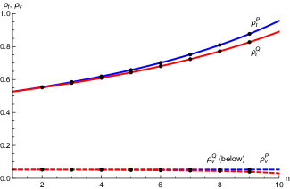
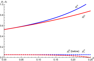
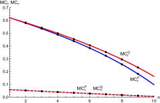
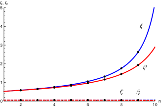
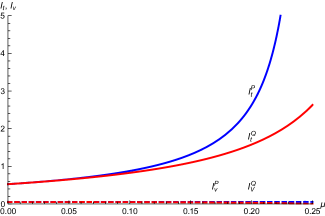
Figure II: Pass-through rate (top), marginal cost of public funds (middle), and incidence (bottom) with linear demand. The horizontal axes on the left and the right panels correspond to the number of firms ($n$) and the substitutability parameter ($\mu$), respectively.

The top two panels in Figure II illustrate how $\rho_{t}$ and $\rho_{v}$ behave as the number of firms ($n$; the left) or the sustainability parameter ($\mu$; the left) increases, with the superscript denoting price ($P$) or quantity ($Q$) setting. Similarly, the middle and the bottom panels draw $MC_{t}$ and $MC_{v}$, and $I_{t}$ and $I_{v}$, respectively. It is observed that the ad valorem tax pass-through rates are close to zero because in this case both $\epsilon_{F}$ and $\eta_{F}$ are close to 1. As competition becomes fiercer, both $\rho_{t}^{P}$ and $\rho_{t}^{Q}$ become larger, although the discrepancy also becomes larger. In the case of linear demand, the difference in the mode of competition does not yield a significant difference in each of the three measures. As is verified by Anderson, de Palma, and Kreider (2001b), the ad valorem tax is more efficient than the unit tax: the dashed lines in the two middle panels lie below the solid lines. This ranking is related inversely to the pass-through and the incidence: as the pass-through or the incidence becomes larger, the marginal cost of public funds becomes smaller.

3.3.2 Logit demand

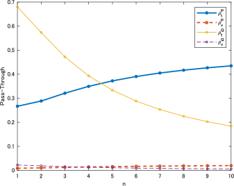
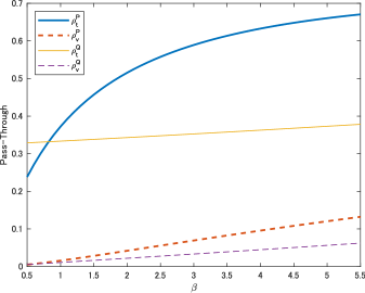
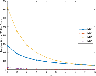
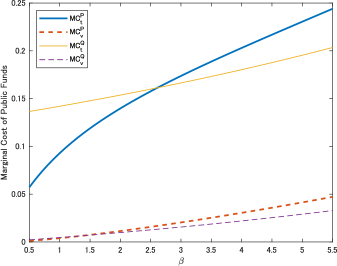
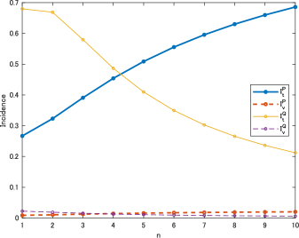
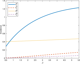
Figure III: Pass-through rates (top), marginal costs of public funds (middle), and incidence (bottom) with logit demands. The horizontal axes on the left and the right panels are the number of firms ($n$) and the price coefficient ($\beta$), respectively.

The next parametric example is the logit demand. Each firm $j=1,...,n$ faces the following demand: $s_{j}(\mathbf{p})=\exp(\delta-\beta p_{j})/[1+\text{$\sum$}_{j\text{\textasciiacute}=1,...,n}\exp(\delta-\beta p_{j\text{\textasciiacute}})]\text{$\in$}(0,1)$, where $\delta$ is the (symmetric) product-specific utility and $\beta>0$ is the responsiveness to the price. We define $s\text{\textsubscript{0}}=1-\text{$\sum$}_{j=1,...,n}s_{j}<1$ as the share of all outside goods. Table I (b) summarizes the key variables that determine the pass-through rates and the marginal costs of public funds. We need to numerically solve for the equilibrium price and market share under both settings to compute the pass-through rate, the marginal cost of public funds, and incidence for all four cases. To focus on the two parameters, $\beta$ and $n$, we assume that $\delta=1$ and $mc=0$. Because $\partial s_{j}(\mathbf{p})/\partial p_{j}|_{\mathbf{p}=\left(p,...,p\right)}=-\beta s(1-s)$, the first-order conditions for the symmetric equilibrium price and the market share satisfy $p-t/(1-v)=1/[\beta(1-s)]$ and $s=\mathrm{\exp}(1-\beta p)/[1+n\exp(1-\beta p)]$. If $p$ and $s$ are solved numerically, then $\epsilon$, $\epsilon_{F}$, $\theta$ and $\alpha$ can also be numerically computed. Next, we consider the inverse demands under quantity competition. Then, as in Berry (1994), firm $j$’s inverse demand is given by $p_{j}(\mathbf{s})=[\delta-\log(s_{j}/s\text{\textsubscript{0}})]/\beta$, which implies that $\partial p_{j}(\mathbf{s})/\partial s_{j}|_{\mathbf{s}=\left(s,...,s\right)}=-[1-(n-1)s]/[\beta s(1-ns)]$. Thus, the first-order conditions for the symmetric equilibrium price and the market share satisfy $p-t/(1-v)=[1-(n-1)s]/[\beta(1-ns)]$ and $p=[1-\mathrm{\log}(s/[1-ns])]/\beta$. Then, as above, $\eta$, $\eta_{F}$, $\theta$ and $\sigma$ are computed by numerically solving the first-order conditions for $p$ and $s$. Interestingly, it is verified that in symmetric equilibrium under quantity setting, $\partial p/\partial n=0$: the equilibrium price is the same irrespective of the number of firms, whereas the individual market share is decreasing in the number of firms: $\partial s/\partial n<0$. On the other hand, both the equilibrium price and market share are decreasing in the price coefficient, $\beta$.

Figure III illustrates the pass-through rate, the marginal cost of public funds, and the incidence, in analogy with Figure II. The right panels now show the variables’ dependence on the price coefficient $\beta$. Overall, as in the case of linear demand, an increase in the ad valorem tax has a small impact on these measures for each of $n$ and $\beta$, whereas an increase in the unit tax has a large effect. However, there are important differences between the cases of linear and logit demand. First, the unit tax pass-through under quantity competition $\rho_{t}^{Q}$ is decreasing in the number of firms. To understand this, compare the difference in the denominators of $\rho_{t}^{P}=1/\{(1-v)\left[1+(1-\alpha/\epsilon_{F})\theta\right]\}$ and $\rho_{t}^{Q}=(1-v)\left[1+\theta-\sigma\right]$. As $\theta$ decreases (i.e., as competition becomes fiercer), the second term in the denominator of $\rho_{t}^{P}$ decreases, and thereby $\rho_{t}^{P}$ increases as $n$ increases. However, $\theta-\sigma$ increases as $\theta$ decreases, and thus $\rho_{t}^{Q}$ decreases. This difference in the denominators is also reflected in the fact that $I_{t}^{Q}$ is decreasing in $n$ as well. Naturally, $MC_{t}^{Q}$ is decreasing in $n$ as in the case of linear demand because $1/\rho_{t}^{Q}$ becomes larger (see the formulas in Proposition 1). Second, while the pass-through rate and the incidence increase as $\beta$ increases, the marginal cost of public funds is also increasing in contrast to the case of linear demands. The reason is that the effect on $MC$ of decreases in $\theta$ is weaker than the effect of the increase in $\epsilon$: the industry’s demand becomes elastic quickly as consumers become more sensitive to a price increase.

4 Multi-Dimensional Pass-Through Framework

Now, we generalize our previous results to a more general specification of taxation that involves multiple tax instruments. We define two different types of pass-through vectors: (i) the pass-through rate vector and (ii) pass-through quasi-elasticity. We study their properties and show that they play a central role in evaluating welfare changes in response to changes in taxation.

4.1 Pass-through, conduct index, and welfare: A general discussion

4.1.1 Generalized pass-through and tax sensitivities

Consider a tax structure under which a firm’s tax payment is expressed as $\phi(p,q,\mathbf{T})$, where $\mathbf{T}\equiv(T_{1},...,T_{d})$ is a $d$-dimensional vector of tax instruments so that the firm’s profit in symmetric equilibrium is written as $\pi=pq-c(q)-\phi(p,q,\mathbf{T})$. Note that the argument so far is a special case of two dimensional pass-through: $\phi(p,q,\mathbf{T})=tq+vpq$, where $\mathbf{T}=(t,v)$. The components of the (per-firm) tax revenue gradient vector $\nabla\phi(p,q,\mathbf{T})$ are

$$\phi_{T_{\ell}}(p,q,\mathbf{T})\equiv\frac{\partial\phi(p,q,\mathbf{T})}{\partial T_{\ell}}.$$

Here, as in other parts of the paper, we use the symbol $\nabla$ for the $d$-dimensional gradient with respect to $\mathbf{T}$. The arguments $p$ and $q$ in $\phi(p,q,\mathbf{T})$ are treated as fixed for the purposes of taking this gradient. We also denote by $\mathbf{f}$ a vector components $\phi_{T_{\ell}}(p,q,\mathbf{T})/q$. We denote the equilibrium price function by $p^{\star}\left(\mathbf{T}\right)$ and its gradient, the pass-through rate vector, by $\tilde{\boldsymbol{\rho}}\equiv\nabla p^{\star}\left(\mathbf{T}\right).$ Further, we use the components of the $\mathbf{f}$ and $\boldsymbol{\tilde{\rho}}$ to define the pass-through quasi-elasticity vector as

$$\boldsymbol{\rho}\equiv\left(\rho_{T_{1}},...,\rho_{T_{d}}\right),\qquad\rho_{T_{\ell}}\equiv\frac{\tilde{\rho}_{T_{\ell}}}{f_{T_{\ell}}}=\frac{q}{\phi_{T_{\ell}}(p,q,\mathbf{T})}\ \frac{\partial p^{\star}}{\partial T_{\ell}}.$$

Note that the components of $\boldsymbol{\rho}$ are all dimensionless. We define the (first-order) price sensitivity $\nu$ of the tax revenue and the (first-order) quantity sensitivity $\tau$ of the (per-firm) tax revenue as follows:

$$\nu(p,q,\mathbf{T})\equiv\frac{1}{q}\phi_{p}(p,q,\mathbf{T}),\qquad\tau(p,q,\mathbf{T})\equiv\frac{1}{p}\phi_{q}(p,q,\mathbf{T}),$$

and their derivatives are

$$\nu_{T_{\ell}}(p,q,\mathbf{T})\equiv\frac{\partial\nu(p,q,\mathbf{T})}{\partial T_{\ell}},\qquad\tau_{T_{\ell}}(p,q,\mathbf{T})\equiv\frac{\partial\tau(p,q,\mathbf{T})}{\partial T_{\ell}}.$$

The analogous definitions for the second-order sensitivities are:

$$\nu_{\text{(2)}}(p,q,\mathbf{T})\equiv\frac{p}{q}\ \frac{\partial^{2}\phi(p,q,\mathbf{T})}{\partial p^{2}},\,\tau_{\text{(2)}}(p,q,\mathbf{T})\equiv\frac{q}{p}\ \frac{\partial^{2}\phi(p,q,\mathbf{T})}{\partial q^{2}},\>\kappa(p,q,\mathbf{T})\equiv\frac{\partial^{2}\phi(p,q,\mathbf{T})}{\partial p\>\partial q}.$$

The first-order and second-order sensitivities are dimensionless, as are the components of $\boldsymbol{\rho}$. In this section, we keep the same definition of the elasticities $\epsilon$ and $\eta$ as before.

4.1.2 Generalized conduct index

We introduce the conduct index $\theta$ as a function, independently of the cost-side of the oligopoly game, so that in equilibrium the following condition holds:

$$\left[1-\tau-\left(1-\nu\right)\eta\,\theta\right]p=mc.$$ (3)

In the case of unit and ad valorem taxation, this definition reduces to the conduct index defined earlier (Equation 1), where $\tau=v+t/p$ and $\nu=v$: this is the reason why we can keep using $\tau$ below. In principle, there are many possible definitions that agree with the earlier definition in the case of unit and ad valorem taxation. However, we find the specification of Equation 3 particularly convenient.

4.1.3 Relationships for the pass-through vector components

We now establish the following relationship for the relative size of pass-through vector component.

Proposition 8.

The pass-through rates and quasi-elasticities satisfy 

$$\frac{\tilde{\rho}_{T_{\ell}}}{\tilde{\rho}_{T_{\ell^{\prime}}}}=\frac{\tau_{T_{\ell^{\prime}}}-\nu_{T_{\ell^{\prime}}}\eta\>\theta}{\tau_{T_{\ell}}-\nu_{T_{\ell}}\eta\>\theta},\qquad\frac{\rho_{T_{\ell}}}{\rho_{T_{\ell^{\prime}}}}=\frac{f_{T_{\ell^{\prime}}}}{f_{T_{\ell}}}\ \frac{\tau_{T_{\ell}}-\eta\>\theta\>\nu_{T_{\ell}}}{\tau_{T_{\ell^{\prime}}}-\eta\>\theta\>\nu_{T_{\ell^{\prime}}}}.$$

The proposition is proven in Appendix A.3.1. Since the components have known proportions, we can write them using a common factor $p\rho_{\left(0\right)}$ as

$$\tilde{\rho}_{T_{\ell}}=\left(\tau_{T_{\ell}}-\nu_{T_{\ell}}\eta\>\theta\right)p\rho_{\left(0\right),}\qquad\rho_{T_{\ell}}=\frac{p}{f_{T_{\ell}}}\left(\tau_{T_{\ell}}-\nu_{T_{\ell}}\eta\>\theta\right)\rho_{\left(0\right),}$$ (4)

with the factor $\rho_{\left(0\right)}$ determined in the following proposition.

Proposition 9.

The value of the factor $\rho_{\left(0\right)}$ introduced in Equation (4) is given by:

$$\frac{1}{\rho_{\left(0\right)}}=1-\kappa+\epsilon\tau_{\left(2\right)}+(1-\tau)\epsilon\chi+\left[\nu-\kappa+\eta\nu_{\left(2\right)}+\left(\omega-\eta-\chi\right)(1-\nu)\right]\theta,$$ (5)

where $\omega\equiv q\>(\eta\theta)^{\prime}/\left(\eta\theta\right),$ with the prime denoting a derivative with respect to the quantity $q.$

The proof is in Appendix A.3.2.

4.1.4 Welfare changes and their relationship to pass-through vectors

Now, we establish the general formulas for the marginal cost of public fund and incidence in the multi-dimensional pass-through framework. Welfare component changes in response to an infinitesimal change in taxes can be found as follows. The (per-firm) consumer surplus change in response to an infinitesimal change $dT_{\ell}$ in the tax $T_{\ell}$ is

$$dCS=-qdp=-q\tilde{\rho}_{T_{\ell}}dT_{\ell},$$

which means that in vector notation, $\frac{1}{q}\,\nabla CS=-\tilde{\boldsymbol{\rho}}$. The change in (per-firm) producer surplus is

$$dPS=d\left(pq-c\left(q\right)-\phi(p,q,\mathbf{T})\right)=\left[\phi_{T_{\ell}}(p,q,\mathbf{T})-\left(1-\nu\right)\left(1-\theta\right)\tilde{\rho}_{T_{\ell}}\right]dT_{\ell},$$

where we utilize Equation (3) to eliminate the marginal cost. In vector notation, this is $\frac{1}{q}\,\nabla PS=\left(1-\nu\right)\left(1-\theta\right)\tilde{\boldsymbol{\rho}}-\mathbf{f}$, since $\mathbf{f}=\frac{1}{q}\nabla\phi(p,q,\mathbf{T})$. The change in tax revenue is

$$dR=\phi_{p}(p,q,\mathbf{T})dp+\phi_{q}(p,q,\mathbf{T})dq+\phi_{T_{\ell}}(p,q,\mathbf{T})dT_{\ell}=\left[\phi_{T_{\ell}}(p,q,\mathbf{T})-\left(\epsilon\tau-\nu\right)\tilde{\rho}_{T_{\ell}}\right]dT_{\ell}.$$

In vector notation, $\frac{1}{q}\,\nabla R=\mathbf{f}-\left(\epsilon\tau-\nu\right)\tilde{\boldsymbol{\rho}}$. Finally, for the change in social welfare, we have

$$dW=\left(p-mc\right)dq=\left[\epsilon\tau+\theta\left(1-\nu\right)\right]\tilde{\rho}_{T_{\ell}}dT_{\ell}.$$

In vector notation, $\frac{1}{q}\,\nabla W=-\left[\epsilon\tau+\theta\left(1-\nu\right)\right]\tilde{\boldsymbol{\rho}}$.

Note that the welfare components $CS\left(\mathbf{T}\right),\ PS\left(\mathbf{T}\right),\>R\left(\mathbf{T}\right)$, and $W\left(\mathbf{T}\right)=CS\left(\mathbf{T}\right)+PS\left(\mathbf{T}\right)+R\left(\mathbf{T}\right)$ are all treated as functions of taxes only and represent the equilibrium outcomes. This is different from the tax revenue function $\phi\left(p,q,\mathbf{T}\right)$, which has also $p$ and $q$ as arguments and which is specified by the government irrespective of the equilibrium. We summarize these findings in the following proposition.

Proposition 10.

The tax gradients of consumer surplus, producer surplus, tax revenue, and social welfare with respect to the taxes all belong to a two-dimensional vector space spanned by $\mathbf{f}$ and $\tilde{\boldsymbol{\rho}}$. The precise linear combinations of $\mathbf{f}$ and $\tilde{\boldsymbol{\rho}}$ are

$$\frac{1}{q}\,\nabla CS=-\tilde{\boldsymbol{\rho},}$$

$$\frac{1}{q}\,\nabla PS=\left(1-\nu\right)\left(1-\theta\right)\tilde{\boldsymbol{\rho}}-\mathbf{f},$$

$$\frac{1}{q}\,\nabla R=\mathbf{f}+\left(\nu-\epsilon\tau\right)\tilde{\boldsymbol{\rho}},$$

$$\frac{1}{q}\,\nabla W=-\left[\left(1-\nu\right)\theta+\epsilon\tau\right]\tilde{\boldsymbol{\rho}}.$$

These relationships, considered component-wise, immediately imply the following results for welfare change ratios and generalize Propositions 1 and 2.

Proposition 11.

The marginal cost of public funds of a tax $T_{\ell}$, $MC_{T_{\ell}}=\left(\nabla W\right)_{T_{\ell}}/\left(\nabla R\right)_{T_{\ell}}$, is

$$MC_{T_{\ell}}=\frac{\left(1-\nu\right)\theta+\epsilon\tau}{\frac{1}{\rho_{T_{\ell}}}+\nu-\epsilon\tau}.$$

The incidence of this tax, $I_{T_{\ell}}=\left(\nabla CS\right)_{T_{\ell}}/\left(\nabla PS\right)_{T_{\ell}}$, equals:

$$I_{T_{\ell}}=\frac{1}{\frac{1}{\rho_{T_{\ell}}}-\left(1-\nu\right)\left(1-\theta\right)}.$$

Similarly, the social incidence, $SI_{T_{\ell}}=\left(\nabla W\right)_{T_{\ell}}/\left(\nabla PS\right)_{T_{\ell}}$, equals:

$$SI_{T_{\ell}}=\frac{\left(1-\nu\right)\theta+\epsilon\tau}{\frac{1}{\rho_{T_{\ell}}}-\left(1-\nu\right)\left(1-\theta\right)}.$$

4.2 Pass-through, conduct index, and welfare: special cases

The results of the previous subsection contain our results for ad valorem and unit taxes as special cases, but provide much greater generality, since the taxes (government interventions) may be specified in a very flexible way.

4.2.1 Exogenous competition and depreciating licenses

Weyl and Fabinger’s (2013) results under symmetric oligopoly can be interpreted as special cases of the present results. In particular, Weyl and Fabinger’s (2013) analysis considers either unit taxes or exogenous competition (an exogenous quantity supplied to the market). The case of unit taxes is clearly included in the present results, which has motivated this paper. At the same time, it turns out that the case of exogenous competition is included as well. The reasoning is as follows.

Consider a tax $T_{1}=\tilde{q}$ of the form: $\phi\left(p,q,\tilde{q}\right)=\tilde{q\,}p+c(\text{$q-\tilde{q}$})-c(q)$. Then, the firm’s profit is given by:

$$pq-c\left(q\right)-\phi\left(p,q,\tilde{q}\right)=p\left(q-\tilde{q}\right)+c(\text{$q-\tilde{q}$}).$$

The firm, therefore, has the same profit function as in the case of exogenous competition $\tilde{q}$ in Weyl and Fabinger (2013). Proposition 11 above (specialized to constant marginal cost and zero initial $\tilde{q}$) then implies the social incidence result in Principle of Incidence 3 in Weyl and Fabinger (2013, p. 548).

Similarly, the relationships between pass-through of unit taxes and of exogenous competition are implied by the general result of Proposition 8 for the tax specification $T_{1}=t$, $T_{2}=\tilde{q}$,

$$\phi\left(p,q,t,\tilde{q}\right)=tq+\tilde{q\,}p+c(\text{$q-\tilde{q}$})-c(q).$$

To obtain the absolute size of the two types of pass-through, one can straightforwardly use Proposition 9. More generally, $\phi$ is extended as

$$\phi=c\left(q-\tilde{q}\right)+v\left(q-\tilde{q}\right)p(q)+(1-v)\tilde{q}p(q)+t\left(q-\tilde{q}\right)-c(q),$$

where an ad valorem tax is also considered. As an example, one can think of a government which procures goods from abroad and supplies them to the market in order to lower domestic prices.

In the special case of a monopolist with constant marginal cost, the mathematics allow for another interesting interpretation: It is isomorphic to the case of “depreciating licenses” in Weyl and Zhang (2017). Depreciating licenses correspond to a tax scheme where the owner of an asset announces a reservation price at which she is willing to sell it and gets taxed a fixed fraction of that prices. Another agent in the economy may buy the asset at the announced price. The owner then faces a tradeoff between announcing a low price and paying low taxes and announcing a high price in order to be able to keep the asset and derive utility from it. The optimization problem then leads to exactly the same mathematical form as the problem of a monopolist with constant marginal cost facing exogenous competition. We include a more detailed explanation in Appendix A.3.3.

4.2.2 Sales restrictions

Governments often regulate when, where, and to whom products may be sold. For example, there are restrictions on weekend sales, store locations, etc. A simple way of modeling this situation is to assume that due to the restrictions a firm loses a fixed proportion of its customers. If the absence of the regulation and taxation, the profit function is $p\left(q\right)q-c\left(q\right)$. The new profit function will be $\left(1-v\right)p([1+\kappa]q)q-tq-c\left(q\right)$, where $1-1/\left(1+\kappa\right)$ is the fraction of customers lost. The only change is in the argument of the inverse demand function: for the firm to sell quantity $q$, each remaining customer needs to buy $\left(1+\kappa\right)$ times more than in the absence of the regulation, and the price would have to be correspondingly lower. This change may be described using as:

$$\phi\left(p,q,t,v,\kappa\right)=\left(1-\left(1-v\right)h\left(q,\kappa\right)\right)pq+tq,\qquad h\left(q,\kappa\right)\equiv\frac{p\left(q\right)-p\left(\left(1+\kappa\right)q\right)}{p\left(q\right)}.$$

For demand with constant elasticity $\epsilon$, $h\left(q,\kappa\right)=1-(1+\kappa)^{-1/\epsilon}$, independently of $q$.

4.2.3 Tax evasion/tax avoidance and concealment costs

Tax evasion, clearly, is a very important problem in many situations since economic agents do not always strictly follow the law (Choi, Furusawa, and Ishikawa 2017).

For simplicity, consider a firm that needs to pay an ad valorem tax $v\tilde{p}q$, where $\tilde{p}$ is the price reported to the government and may differ from the true price $p$. We capture the cost associated with deceiving the government by introducing a concealment cost of the form:

$$\frac{1}{4\lambda}p^{-\zeta}(\tilde{p}-p)^{2}q^{1-\xi}.$$

The firm then chooses the reported price $\tilde{p}$ to minimize the sum of these two additional costs:

$$v\tilde{p}q+\frac{1}{4\lambda}p^{-\zeta}q^{1-\xi}(\tilde{p}-p)^{2}.$$

The corresponding first-order condition implies $\tilde{p}=p-2\lambda vp^{\zeta}q^{\xi}$, which gives the effective additional cost

$$pqv-\lambda v^{2}p^{\zeta}q^{1+\xi}.$$

$$\phi\left(p,q,t,v,\lambda\right)=tq+pqv-\lambda v^{2}p^{\zeta}q^{1+\xi}$$

$$\tilde{\phi}\left(p,q,t,v,\lambda\right)=tq+pqv-2\lambda v^{2}p^{\zeta}q^{1+\xi}$$

The government needs to pay additional enforcement cost inversely related to $\lambda$, which needs to be remembered in the welfare analysis.

5 Heterogeneous Firms

In this section, we extend our results to the case of $n$ heterogeneous firms (i.e. asymmetric firms), where each firm $i$ controls a strategic variable $\sigma_{i}$, which could be, for example, the price or quantity of its product. We allow for the tax function $\phi_{i}\left(p_{i},q_{i},\mathbf{T}\right)$ to depend explicitly on the identity of the firm; we write $f_{i\>T_{\ell}}\left(p_{i},q_{i},\mathbf{T}\right)=\frac{1}{q_{i}}\,\frac{\partial}{\partial T_{\ell}}\phi_{i}\left(p_{i},q_{i},\mathbf{T}\right)$ for its derivative with respect to tax $T_{\ell}$. Similarly, the sensitivities $\tau_{i}\left(p_{i},q_{i},\mathbf{T}\right)$, $\nu_{i}\left(p_{i},q_{i},\mathbf{T}\right)$, etc., now also have the firm index $i$. The marginal cost $mc_{i}\left(q_{i}\right)$ of firm $i$ is also allowed to depend on the identity of the firm, and we denote its elasticity $\chi_{i}\left(q_{i}\right)\equiv q_{i}\,mc_{i}^{\prime}\left(q_{i}\right)/mc_{i}\left(q_{i}\right).$

5.1 Pricing strength index and pass-through

We define the pricing strength index $\psi_{i}\left(\mathbf{q}\right)$ of firm $i$ to be a function independent of the cost side of the economic problem such that the first-order condition for firm $i$ is:

$$\left\{1-\tau_{i}\left(p_{i}\left(\mathbf{q}\right),q_{i},\mathbf{T}\right)-\psi_{i}\left(\mathbf{q}\right)\left[1-\nu_{i}\left(p_{i}\left(\mathbf{q}\right),q_{i},\mathbf{T}\right)\right]\right\}p_{i}\left(\mathbf{q}\right)=mc\left(q_{i}\right).$$

In the special case of symmetric firms, this definition reduces to $\psi_{i}=\eta\,\theta$.

We express the pass-through rate in terms of these pricing strength indices. Specifically, the pass-through rate is an $n\times d$ matrix $\mathbf{\tilde{\rho}}$ with rows $\tilde{\mathbf{\boldsymbol{\rho}}}_{T_{\ell}}\equiv\partial\mathbf{p}/\partial T_{\ell}$ and elements $\tilde{\rho}_{i\,T_{\ell}}=\partial p_{i}/\partial T_{\ell}$. It is shown that the pass-through rate equals

$$\tilde{\mathbf{\rho}}_{T_{\ell}}=\mathbf{b}^{-1}\,.\,\mathbf{\iota}_{T_{\ell}},$$ (6)

where the factors on the right-hand side are defined as follows. The matrix $\mathbf{b}$ is an $n\times n$ matrix, independent of the choice of $T_{\ell}$, with elements

$$b_{ij} = \left[1-\kappa_{i}-\left(1-\nu_{i}-\nu_{\text{(2)}i}\right)\!\psi_{i}\right]\delta_{ij}-\left(1-\nu_{i}\right)\!\psi_{i}\Psi_{ij}$$

$$+ \left\{\tau_{\text{(2)}i}+\nu_{i}\psi_{i}-\kappa_{i}+\left[1-\tau_{i}-\left(1-\nu_{i}\right)\psi_{i}\right]\!\chi_{i}\right\}\epsilon_{ij},$$

where $\delta_{ij}$ is the Kronecker delta, and

$$\epsilon_{ij}=-\,\frac{p_{i}}{q_{i}}\,\frac{\partial q_{i}\left(\mathbf{p}\right)}{\partial p_{j}},\qquad\Psi_{ij}=\frac{p_{i}}{\psi_{i}}\frac{\partial\psi_{i}\left(\mathbf{q}\left(\mathbf{p}\right)\right)}{\partial p_{j}}.$$

For each tax $T_{\ell}$, $\mathbf{\iota}_{T_{\ell}}$ is an $n$-dimensional vector with components

$$\iota_{i\,T_{\ell}}=p_{i}\,\frac{\partial\tau_{i}\left(p_{i},q_{i},\mathbf{T}\right)}{\partial T_{\ell}}-p_{i}\,\psi_{i}\,\frac{\partial\nu_{i}\left(p_{i},q_{i},\mathbf{T}\right)}{\partial T_{\ell}}.$$

In the case of symmetric firms and at symmetric prices, the pass-through rate expression in Equation (6) agrees with the expression represented by Equations (4) and (5) in Section 4.

To generalize the notion of pass-through quasi-elasticity to the case of heterogeneous firms, we define the pass-through quasi-elasticity matrix $\mathbf{\rho}$ as an $n\times d$ matrix with elements

$$\rho_{i\,T_{\ell}}=\frac{1}{f_{i\,T_{\ell}}\left(p_{i},q_{i},\mathbf{T}\right)}\ \frac{\partial p_{i}}{\partial T_{\ell}},$$

and with rows denoted $\mathbf{\rho}_{T_{\ell}}$.

5.2 Welfare changes

In the following, for each $i$, $\mathbf{\epsilon}_{i}$ is an $n$-dimensional vector with its $j$-th component equal to $\epsilon_{ij}$. For the tax gradients of welfare components corresponding to individual firms we obtain:

$$\frac{1}{q_{i}}\nabla CS_{i}=-\mathbf{e}_{i}.\tilde{\boldsymbol{\rho},}$$

$$\frac{1}{q_{i}}\nabla PS_{i}=\left(1-\nu_{i}\right)\left(\mathbf{e}_{i}-\psi_{i}\,\mathbf{\epsilon}_{i}\right).\tilde{\boldsymbol{\rho}}-\mathbf{f}_{i},$$

$$\frac{1}{q_{i}}\nabla R_{i}=\mathbf{f}_{i}+\left(\nu_{i}\,\mathbf{e}_{i}-\tau_{i}\,\mathbf{\epsilon}_{i}\right).\tilde{\boldsymbol{\rho}},$$

$$\frac{1}{q_{i}}\nabla W_{i}=-\left[\tau_{i}+\psi_{i}\>\left(1-\nu_{i}\right)\right]\mathbf{\epsilon}_{i}.\tilde{\boldsymbol{\rho}}.$$

The corresponding gradients of total welfare components are then obtained by adding up contributions from individual firms. For example, $\nabla CS=\sum_{i=1}^{n}\nabla CS_{i}$. Denoting the total quantity as $Q\equiv\sum_{i=1}^{n}q_{i}$, this means that $\frac{1}{Q}\nabla CS$ is a weighted average of $-\mathbf{e}_{i}.\tilde{\boldsymbol{\rho}}$, with the weights proportional to $q_{i}$. The arguments for the other welfare components are similar. This generalizes Proposition 10 above.

We can also consider ratios of welfare changes corresponding to some tax $T_{\ell}$:

$$MC_{i\,T_{\ell}}=\frac{\left[\tau_{i}+\left(1-\nu_{i}\right)\,\psi_{i}\right]\,\epsilon_{i\,T_{\ell}}^{\rho}}{\frac{1}{\rho_{i\,T_{\ell}}}+\nu_{i}-\tau_{i}\,\epsilon_{i\,T_{\ell}}^{\rho}},$$

$$I_{i\,T_{\ell}}=\frac{1}{\frac{1}{\rho_{i\,T_{\ell}}}-\left(1-\nu_{i}\right)(1-\psi_{i}\,\epsilon_{i\,T_{\ell}}^{\rho})},$$

$$SI_{i\,T_{\ell}}=\frac{\left[\tau_{i}+\left(1-\nu_{i}\right)\,\psi_{i}\right]\,\epsilon_{i\,T_{\ell}}^{\rho}}{\frac{1}{\rho_{i\,T_{\ell}}}-\left(1-\nu_{i}\right)(1-\psi_{i}\,\epsilon_{i\,T_{\ell}}^{\rho})},$$

where $\epsilon_{i\,T_{\ell}}^{\rho}\equiv\mathbf{\epsilon}_{i}.\tilde{\boldsymbol{\rho}}_{T_{\ell}}/\tilde{\rho}_{i\,T_{\ell}}=\mathbf{\epsilon}_{i}.\boldsymbol{\rho}_{T_{\ell}}/\rho_{i\,T_{\ell}}.$ The ratios of the corresponding total welfare changes will be weighted averages of these firm-specific ratios. The weights correspond to the sizes of the denominators times $q_{i}$. For example, $MC_{T_{\ell}}$ will lie between $\min_{i}MC_{i\,T_{\ell}}$ and $\max_{i}MC_{i\,T_{\ell}}$. The same reasoning also holds for the other ratios. This generalizes Proposition 11 above.

5.3 Conduct index and welfare changes

For heterogeneous firms, we introduce the conduct index of firm $i$ so that

$$\theta_{i}=-\frac{\sum_{j=1}^{n}\left\{p_{j}\left[1-\tau_{j}\left(p_{j},q_{j},\mathbf{T}\right)\right]-mc\left(q_{j}\right)\right\}\frac{dq_{j}}{d\sigma_{i}}}{\sum_{j=1}^{n}\left[1-\nu_{j}\left(p_{j},q_{j},\mathbf{T}\right)\right]q_{j}\,\frac{dp_{j}}{d\sigma_{i}}}$$

holds. In the special case of only unit taxation, this definition reduces to Weyl and Fabinger’s (2013, p. 552) Equation (4). In the special case of symmetric firms the definition reduces to our Equation (3) with $\theta_{i}=\theta$.

The conduct index $\theta_{i}$ is closely connected to the pricing strength index $\psi_{i}$, but not as closely as it would be in the case of symmetric oligopoly. Using the definitions of the indices, it is shown that

$$\theta_{i}=-\frac{\sum_{j=1}^{n}\left(1-\nu_{j}\right)\psi_{j}\,p_{j}\frac{dq_{j}}{d\sigma_{i}}}{\sum_{j=1}^{n}\left(1-\nu_{j}\right)q_{j}\frac{dp_{j}}{d\sigma_{i}}}.$$

For symmetric oligopoly, this equation reduces simply to $\theta=\epsilon\psi.$

The conduct index is used to express welfare component changes in response to infinitesimal changes in taxes. The relationships are a bit more complicated than in the case of using the pricing strength index: they can be expressed as follows. We define the price response to an infinitesimal change in the strategic variable $\sigma_{k}$ of firm $j$ as

$$\zeta_{ij}=\frac{dp_{i}}{d\sigma_{j}}.$$

Since the vectors $\zeta_{i1}$, $\zeta_{i2}$, … , $\zeta_{in}$ form a basis in the $n$-dimensional vector space to which $\tilde{\rho}_{i\,T_{\ell}}$ for a given $\ell$ belongs, we can write $\tilde{\rho}_{i\,T_{\ell}}$ as a linear combination of them for some coefficients $\lambda_{i\,T_{\ell}}$:

$$\tilde{\rho}_{i\,T_{\ell}}=\sum_{j=1}^{n}\lambda_{j\,T_{\ell}}\zeta_{ij}.$$

For changes in consumer and producer surplus, we obtain:

$$\frac{dCS}{dT_{\ell}}=-\sum_{i=1}^{n}q_{i}\tilde{\rho}_{i\,T_{\ell}}=-\sum_{j=1}^{n}\left(\sum_{i=1}^{n}q_{i}\zeta_{ij}\right)\lambda_{j\,T_{\ell}},$$

$$\frac{dPS}{dT_{\ell}}=-\sum_{i=1}^{n}f_{i\,T_{\ell}}\left(p_{i},q_{i},\mathbf{T}\right)-\sum_{j=1}^{n}\hat{\zeta}_{j}\,\left(1-\theta_{j}\right)\lambda_{j\,T_{\ell}},$$

where we used the notation

$$\hat{\zeta}_{j}\equiv\sum_{i=1}^{n}\left[1-\nu_{i}\left(p_{i},q_{i},\mathbf{T}\right)\right]q_{i}\,\zeta_{ij}.$$

These surplus change expressions represent a generalization of the surplus expressions in Weyl and Fabinger’s (2013) Section 5.

5.4 Aggregative games

In the case of oligopoly in the form of aggregative games, where all other firms’ actions are summarized as an aggregator in each firm’s profit, we can further manipulate the above formulas for pricing strength and conduct indices. We identify the firm’s strategic variable $\sigma_{i}$ with an action $a_{i}\equiv\sigma_{i}$ the firm can take, which contributes to an aggregator $A=\sum_{i=1}^{n}a_{i}$. The prices and quantities are functions of just two arguments: $p_{i}\left(A,a_{i}\right)$ and $q_{i}\left(A,a_{i}\right)$. Their derivatives that take into account the dependence of $A$ on the action of firm $i$ are $\frac{dq_{j}}{d\sigma_{i}}=\frac{\partial q_{j}}{\partial a_{i}}+\frac{\partial q_{j}}{\partial A}$ and $\frac{dp_{j}}{d\sigma_{i}}=\frac{\partial p_{j}}{\partial a_{i}}+\frac{\partial p_{j}}{\partial A}$. The firm’s first-order condition is:

$$0=\left(\frac{\partial p_{j}}{\partial a_{i}}\left(A,a_{i}\right)+\frac{\partial p_{j}}{\partial A}\left(A,a_{i}\right)\right)q_{i}\left(A,a_{i}\right)\left(\nu_{i}\left(p_{i}\left(A,a_{i}\right),q_{i}\left(A,a_{i}\right),\mathbf{T}\right)-1\right)+\qquad\qquad\qquad$$

$$\qquad\left(\frac{\partial q_{j}}{\partial a_{i}}\left(A,a_{i}\right)+\frac{\partial q_{j}}{\partial A}\left(A,a_{i}\right)\right)\left(mc\left(q_{i}\left(A,a_{i}\right)\right)+p_{i}\left(A,a_{i}\right)\left(\tau_{i}\left(p_{i}\left(A,a_{i}\right)\!,\!q_{i}\left(A,a_{i}\right)\!,\!\mathbf{T}\right)-1\right)\right),$$

which gives us a relatively simple expression for the pricing strength index:

$$\psi_{i}\left(A,a_{i}\right)=-\frac{q_{i}\left(A,a_{i}\right)}{p_{i}\left(A,a_{i}\right)}\ \ \frac{\frac{\partial p_{j}}{\partial a_{i}}\left(A,a_{i}\right)+\frac{\partial p_{j}}{\partial A}\left(A,a_{i}\right)}{\frac{\partial q_{j}}{\partial a_{i}}\left(A,a_{i}\right)+\frac{\partial q_{j}}{\partial A}\left(A,a_{i}\right)}.$$

The expression for the conduct index also simplifies:

$$\theta_{i}=\sum_{j=1}^{n}w_{j}\ \frac{\gamma_{j}\left(A,a_{i}\right)}{\gamma_{j}\left(A,a_{j}\right)},$$

where $w_{i}$ is a normalized version of unnormalized “weights” $\tilde{w}_{j}$,

$$w_{i}\equiv\frac{\tilde{w}_{i}}{\sum_{j=1}^{n}\tilde{w}_{j}},\qquad\tilde{w}_{j}\equiv\left(1-\nu_{j}\right)q_{j}\left(A,a_{j}\right)\,\left(\frac{\partial p_{j}}{\partial a_{i}}\left(A,a_{i}\right)+\frac{\partial p_{j}}{\partial A}\left(A,a_{i}\right)\right),$$

and

$$\gamma_{j}\left(A,a_{i}\right)\equiv\frac{\partial q_{j}}{\partial a_{i}}\left(A,a_{i}\right)+\frac{\partial q_{j}}{\partial A}\left(A,a_{i}\right).$$

These simplified formulas would be used for further analysis of pass-through and welfare in aggregative oligopoly games.

6 Pass-Through and Welfare under Production-Cost and Taxation Changes

In the previous sections, we have studied changes in taxation, but not changes in production costs. Here, we generalize our main results to incorporate both taxation and production costs. As shown below, the generalization to production cost changes turns out to be straightforward. These more general formulas may be applied to a range of economic situations such as cost changes due to exchange rate movements or movements in the world prices of commodities.

The additional cost to the firm is denoted $\phi\left(p,q,\mathbf{T}\right)$ as before, but the tax bill of firm $i$, denoted $\tilde{\phi}\left(p,q,\mathbf{T}\right)$, is different, in general. Here $\mathbf{T}$ is a vector of interventions (by the government or by external circumstances), which may or may not include traditional taxes. We recover the previous case of only taxation by setting $\tilde{\phi}\left(p,q,\mathbf{T}\right)=\phi\left(p,q,\mathbf{T}\right)$. If all of the additional cost to the firm comes from the production side, we have $\tilde{\phi}\left(p,q,\mathbf{T}\right)=0$. In general, $\phi\left(p,q,\mathbf{T}\right)-\tilde{\phi}\left(p,q,\mathbf{T}\right)$ is the production part of the additional cost $\phi\left(p,q,\mathbf{T}\right)$.

6.1 Symmetric firms

In addition to the notation used in the previous section, we define $\tilde{\mathbf{f}}=\frac{1}{q}\nabla\tilde{\phi}(p,q,\mathbf{T})$. First, we obtain a generalization of the formulas for the tax gradients of welfare components in Proposition 10. The equilibrium outcome depends only on the additional cost $\phi\left(p,q,\mathbf{T}\right)$ and not on its split between taxes and production costs. For this reason, the formulas for consumer and producer surplus will be unchanged. The government revenue and therefore also total social welfare depends on $\tilde{\phi}\left(p,q,\mathbf{T}\right)$. In the formula for the gradient of government revenue, $\mathbf{f}$ will be replaced by $\tilde{\mathbf{f}}$, and the formula for social welfare will be adjusted to reflect this difference. Hence, the generalization of the results in Proposition 10 is:

$$\frac{1}{q}\,\nabla CS=-\tilde{\boldsymbol{\rho},}$$

$$\frac{1}{q}\,\nabla PS=\left(1-\nu\right)\left(1-\theta\right)\tilde{\boldsymbol{\rho}}-\mathbf{f},$$

$$\frac{1}{q}\,\nabla R=\mathbf{\tilde{f}}+\left(\nu-\epsilon\tau\right)\tilde{\boldsymbol{\rho}},$$

$$\frac{1}{q}\,\nabla W=-[\left(1-\nu\right)\theta+\epsilon\tau]\tilde{\boldsymbol{\rho}}+\mathbf{\tilde{f}}-\mathbf{f}.$$

We further define $g_{T_{\ell}}\equiv\tilde{f}_{T_{\ell}}/f_{T_{\ell}}$, which represents the fraction of an increase in additional cost ($\phi$) to the firm (due to a change in the tax parameter $T_{\ell}$) that is collected by the government in the form of taxes ($\tilde{\phi}$). In other words, $g_{T_{\ell}}$ is the government’s share in increases of the additional costs induced by marginal changes in $T_{\ell}$. If $\phi$ is a pure tax, then $g_{T_{\ell}}=1$, and if $\phi$ is a pure production cost with no tax component, then $g_{T_{\ell}}=0$. By taking ratios of the components of the tax gradients above, we obtain a generalization of Proposition 11: The marginal cost of public funds associated with intervention $T_{\ell}$, $MC_{T_{\ell}}=\left(\nabla W\right)_{T_{\ell}}/\left(\nabla R\right)_{T_{\ell}}$, is

$$MC_{T_{\ell}}=\frac{\frac{1-g_{T_{\ell}}}{\rho_{T_{\ell}}}+\left(1-\nu\right)\theta+\epsilon\tau}{\frac{g_{T_{\ell}}}{\rho_{T_{\ell}}}+\nu-\epsilon\tau}.$$

The incidence of this intervention, $I_{T_{\ell}}=\left(\nabla CS\right)_{T_{\ell}}/\left(\nabla PS\right)_{T_{\ell}}$, equals:

$$I_{T_{\ell}}=\frac{1}{\frac{1}{\rho_{T_{\ell}}}-\left(1-\nu\right)\left(1-\theta\right)}.$$

Similarly, the social incidence, $SI_{T_{\ell}}=\left(\nabla W\right)_{T_{\ell}}/\left(\nabla PS\right)_{T_{\ell}}$, equals:

$$SI_{T_{\ell}}=\frac{\frac{1-g_{T_{\ell}}}{\rho_{T_{\ell}}}+\left(1-\nu\right)\theta+\epsilon\tau}{\frac{1}{\rho_{T_{\ell}}}-\left(1-\nu\right)\left(1-\theta\right)}.$$

6.2 Heterogeneous firms

The adjustments to our formulas needed to generalize the results of Subsection 5.2 are analogous to the case of symmetric firms we just discussed. For each firm $i$, we define $\tilde{\mathbf{f}}_{i}=\frac{1}{q}\nabla\tilde{\phi}_{i}(p,q,\mathbf{T}).$ For the welfare gradients, we obtain:

$$\frac{1}{q_{i}}\nabla CS_{i}=-\mathbf{e}_{i}.\tilde{\boldsymbol{\rho},}$$

$$\frac{1}{q_{i}}\nabla PS_{i}=\left(1-\nu_{i}\right)\left(\mathbf{e}_{i}-\psi_{i}\,\mathbf{\epsilon}_{i}\right).\tilde{\boldsymbol{\rho}}-\mathbf{f}_{i},$$

$$\frac{1}{q_{i}}\nabla R_{i}=\left(\nu_{i}\,\mathbf{e}_{i}-\tau_{i}\,\mathbf{\epsilon}_{i}\right).\tilde{\boldsymbol{\rho}}+\mathbf{\tilde{f}}_{i},$$

$$\frac{1}{q_{i}}\nabla W_{i}=-\left[\tau_{i}+\psi_{i}\>\left(1-\nu_{i}\right)\right]\mathbf{\epsilon}_{i}.\tilde{\boldsymbol{\rho}}+\mathbf{\tilde{f}}_{i}-\mathbf{f}_{i}.$$

Similarly, for each firm $i$, we define $g_{i\,T_{\ell}}\equiv\tilde{f}_{i\,T_{\ell}}/f_{i\,T_{\ell}}$. For the firm-specific welfare change ratios, we obtain:

$$MC_{i\,T_{\ell}}=\frac{\frac{1-g_{i\,T_{\ell}}}{\rho_{i\,T_{\ell}}}+(\tau_{i}+\left(1-\nu_{i}\right)\,\psi_{i})\,\epsilon_{i\,T_{\ell}}^{\rho}}{\frac{g_{i\,T_{\ell}}}{\rho_{i\,T_{\ell}}}+\nu_{i}-\tau_{i}\,\epsilon_{i\,T_{\ell}}^{\rho}},$$

$$I_{i\,T_{\ell}}=\frac{1}{\frac{1}{\rho_{i\,T_{\ell}}}-\left(1-\nu_{i}\right)(1-\psi_{i}\,\epsilon_{i\,T_{\ell}}^{\rho})},$$

$$SI_{i\,T_{\ell}}=\frac{\frac{1-g_{T_{\ell}}}{\rho_{i\,T_{\ell}}}+(\tau_{i}+\left(1-\nu_{i}\right)\,\psi_{i})\,\epsilon_{i\,T_{\ell}}^{\rho}}{\frac{1}{\rho_{i\,T_{\ell}}}-\left(1-\nu_{i}\right)(1-\psi_{i}\,\epsilon_{i\,T_{\ell}}^{\rho})}.$$

7 Concluding Remarks

In this paper, we characterize the welfare measures of taxation and other external changes in oligopoly with a general specification of competition, market demand and production cost. For symmetric oligopoly, we first derive formulas for marginal welfare losses from unit and ad valorem taxation, $MC_{t}$ and $MC_{v}$, using the unit tax pass-through rate $\rho_{t}$ and the ad valorem tax pass-through semi-elasticity $\rho_{v}$ (Proposition 1) as well as the formulas for tax incidence, $I_{t}$ and $I_{v}$ (Proposition 2). We then show that $\rho_{v}$ can be expressed in terms of $\rho_{t}$ (Proposition 3). These relationships are used to derive sufficient statistics for $MC_{t}$ and $MC_{v}$ (Proposition 4). The pass-through is also characterized, generalizing Weyl and Fabinger’s (2013) formula (Proposition 5). In the case of price or quantity competition, we explain how $\rho_{t}$ and $\rho_{v}$ can be written only in terms of the demand elasticities, the demand curvatures, and the marginal cost elasticity (Propositions 6 and 7). We have discussed the relationships to other quantities of interest, as well as illustrative special cases.

The second part of the paper extends the results beyond the two-dimensional taxation problem. Specifically, we show that the previous results have a very natural generalization to a general specification of the tax revenue function as a function parameterized by a vector of tax parameters (Propositions 8, 9, 10, and 11). We further discuss an extension of our analysis to the case of asymmetric oligopoly, where the firms face different costs and possibly also different taxes (Section 5).^, In addition, we provide a generalization of our results to the case of changes in both production costs and taxes (Section 6).

As already mentioned above, it would be possible to extend our analysis to the case of supply chains (Peitz and Reisinger 2014). Other possible directions include the case of two-sided platform competition (White and Weyl 2016; and Tremblay 2018) and the case of the interactive effects of taxation for multiple imperfectly competitive product markets. In addition, our methodology could be utilized to study other important issues of pricing in general such as the welfare effects of oligopolistic third-degree price discrimination (Adachi and Fabinger 2018). One may also study, for example, advertising pass-through (Draganska and Vitorino 2017). Free-riding, because of the spillover effect, may be more or less serious, depending on the conduct index and other related indices. Furthermore, it would be of interest to develop flexible, but analytically solvable examples along the lines of Fabinger and Weyl (2018).

Appendix A Appendix

A.1 Proofs and discussions for Section 2

A.1.1 Proof of Proposition 1

Using Equation (1) to substitute for $mc$, we first obtain a useful expression for the markup: $p-mc=t+pv+p(1-v)\eta\theta$. Now consider an infinitesimal change $dt$ in the unit tax that induces a change $dp$ in the equilibrium price and a change $dq$ in the equilibrium quantity. These are related by $dt=dp/\rho_{t}=-\eta\thinspace p\thinspace dq/\left(q\thinspace\rho_{t}\right)$. The corresponding change in social welfare per firm is $dW=\left(p-mc\right)dq=t\thinspace dq+vp\thinspace dq+(1-v)p\eta\theta\thinspace dq$, and the change in tax revenue per firm is $dR=\left(t+vp\right)dq+vq\thinspace dp+q\thinspace dt=\left(t+vp\right)dq-vp\eta\thinspace dq-\eta p\thinspace dq/\rho_{t}$. Combining these relationships gives the result

$$MC_{t}=-\frac{dW}{dR}=-\frac{t+vp+(1-v)p\eta\theta}{t+vp-vp\eta-\frac{1}{\rho_{t}}p\eta}=\frac{(1-v)\eta\theta+\frac{t}{p}+v}{\frac{1}{\rho_{t}}\eta+v\eta-\frac{t}{p}-v}=\frac{(1-v)\theta+\epsilon\tau}{\frac{1}{\rho_{t}}+v-\epsilon\tau}.$$

Next, consider an infinitesimal change $dv$ in the ad valorem tax that induces a change $dp$ in the equilibrium price and a change $dq$ in the equilibrium quantity, related by $dv=dp/(p\rho_{v})=-\eta\,dq/(q\rho_{v})$. The change in social welfare per firm is again $dW=\left(p-mc\right)dq=t\,dq+vp\,dq+(1-v)p\eta\theta\,dq$. The change in tax revenue per firm can be written as $\left(t+vp\right)dq+vq\,dp+pq\,dv=\left(t+vp\right)dq-vp\eta\,dq-p\eta\,dq/\rho_{v}$. Combining these relationships leads to the result

$$MC_{t}=-\frac{dW}{dR}=-\frac{t+vp+(1-v)p\eta\theta}{t+vp-vp\eta-\frac{1}{\rho_{v}}p\eta}=\frac{(1-v)\eta\theta+\frac{t}{p}+v}{\frac{1}{\rho_{v}}\eta+v\eta-\frac{t}{p}-v}=\frac{(1-v)\theta+\epsilon\tau}{\frac{1}{\rho_{v}}+v-\epsilon\tau}.$$

A.1.2 Intuition behind Proposition 1

The intuition behind Proposition 1 for the case of unit taxation can explained as follows. The argument for ad valorem taxation is analogous. First, the firm’s per-output profit margin is decomposed into two parts: (1) tax payment, $t+vp=p\tau$ and (2) surplus from imperfect competition, $(1-v)p\eta\theta$. Under imperfect competition, the effects of an increase in unit tax, $dt$, on the social welfare can be written as $dW=(p-mc)dq$, which implies that the firm’s per-output profit margin serves as a measure for welfare change. On the other hand, the effects of an increase in unit tax, $dt$, on the tax revenue are:

$$dR=\underset{(1)>0}{\underbrace{q\,dt}}+\underset{(2)>0}{\underbrace{vq\,dp}}+\underset{(3)<0}{\underbrace{(t+vp)dq}},$$

where term (1) expresses (direct) gain, multiplied by the output $q$, and term (2) shows (indirect) gain, due to the associated price increase, multiplied by $vq$, whereas term (3) is the part that exhibits (indirect) loss from the output reduction for both unit tax revenue and ad valorem tax revenue. Now recall that $dp=\rho_{t}dt$ and $p\eta dq=-qdp$. Thus, $qdt=qdp/\rho_{t}=-(p\eta/\rho_{t})dq$ and $vqdp=-(vqp/q)\eta dq=-(vp\eta)dq$, which implies that

$$dR=-(p\eta/\rho)dq-(vp\eta)dq+(t+vp)dq=[\underset{(1)\thinspace>0}{\underbrace{\left(-p\eta/\rho_{t}\right)}}+\underset{(2)\thinspace>0}{\underbrace{(-vp\eta)}}+\underset{(3)\thinspace<0}{\underbrace{(t+vp)}}].$$

Now, in the per-price term, the denominator and the numerator in $MC_{t}$ are expressed as follows:

$$MC_{t}=\frac{\underset{\textrm{welfare}\thinspace\textrm{loss}\thinspace\textrm{expressed}\thinspace\textrm{by}\thinspace\textrm{the}\thinspace\textrm{profit}\thinspace\textrm{margin}}{\underbrace{(1-v)\eta\theta+\tau}}}{\underset{\textrm{revenue}\thinspace\textrm{gain}}{\underbrace{\left(\frac{1}{\rho_{t}}+v\right)\eta}}+\underset{\textrm{revenue}\thinspace\textrm{loss}}{\underbrace{(-\tau)}}}.$$

A.1.3 Proof of Proposition 2

The impact of a change $dt$ in the tax $t$ on consumer surplus (per firm) is $dCS=-qdp=-q\rho_{t}dt$. The impact on producer surplus is

$$dPS=d[\left(1-v\right)pq-c\left(q\right)-tq]=-q\,dt+\left(1-v\right)p\,dq+\left(1-v\right)qdp-mc\,dq-t\,dq,$$

$$\Leftrightarrow dPS=-qdt+\left(1-v\right)q\rho_{t}dt+[\left(1-v\right)p-mc-t]dq.$$

Substituting for $mc$ from Equation (1) as $mc=\left(1-v\right)\left(1-\eta\theta\right)p-t$ gives

$$dPS=-qdt+\left(1-v\right)q\rho_{t}dt+\left(1-v\right)\eta\theta pdq=-qdt+\left(1-v\right)q\rho_{t}dt-\left(1-v\right)\theta qdp,$$

$$\Leftrightarrow dPS=-qdt+\left(1-v\right)q\rho_{t}dt-\left(1-v\right)\theta q\rho_{t}dt=-[1-\left(1-v\right)\left(1-\theta\right)\rho_{t}]q\,dt.$$

The reciprocal of the incidence ratio is

$$\frac{1}{I_{t}}=\frac{dPS}{dCS}=\frac{\left(1-v\right)\left(1-\theta\right)q\rho_{t}-q}{-q\rho_{t}}=\frac{1}{\rho_{t}}-\left(1-v\right)\left(1-\theta\right).$$

For infinitesimal changes in ad valorem taxes, we proceed analogously. The change in consumer surplus is $dCS=-qdp=-qp\rho_{v}dv.$ For the change in producer surplus we have

$$dPS=d\left(\left(1-v\right)pq-c\left(q\right)-tq\right)=-pq\,dv+\left(1-v\right)p\,dq+\left(1-v\right)qdp-mc\,dq-t\,dq.$$

Manipulating the last four terms on the right-hand side in the same way as before leads to

$$dPS=-pq\,dv+\left(1-v\right)p\,dq+\left(1-v\right)qdp-mc\,dq-t\,dq,$$

$$dPS=-pq\,dv+\left(1-v\right)qp\rho_{v}dv-\left(1-v\right)\theta qp\rho_{v}dv=\left[\left(1-v\right)\left(1-\theta\right)\rho_{v}-1\right]qp\,dv.$$

The reciprocal of the incidence ratio then becomes

$$\frac{1}{I_{t}}=\frac{dPS}{dCS}=\frac{\left(1-v\right)\left(1-\theta\right)\rho_{v}q-q}{-q\rho_{v}}=\frac{1}{\rho_{v}}-\left(1-v\right)\left(1-\theta\right).$$

A.1.4 Intuition behind Proposition 2

The intuitive reasoning behind Proposition 2 can be provided as follows. First, the effects of an increase in unit tax, $dt$, on the producer surplus can be decomposed into the following five parts:

$$dPS=\underset{(1)<0}{[\underbrace{(-q\,dt)}}+\underset{(2)<0}{\underbrace{(1-v)p\,dq}}]+\underset{(3)>0}{[\underbrace{(1-v)q\,dp}}+\underset{(4)>0}{\underbrace{(-mc\,dq)}}+\underset{(5)>0}{\underbrace{(-t\,dq)}}],$$

where term (1) shows the (direct) loss from an increase in unit tax: the tax increase multiplied by the output $q$, and term (2) is another (indirect) loss from a reduction in production, multiplied by the ad valor em tax adjusted unit price $(1-v)p$, whereas term (3) corresponds to the (direct) gain from the associated price increase, mitigated by $(1-v)$, due to the ad valorem tax, multiplied by the output $q$, and finally terms (4) and (5) are (indirect) gains from cost savings by the output reduction, $dq$, and from unit tax saving by the output reduction, $dq$, respectively. Note here that the equation above is rewritten as

$$dPS=\underset{(1)<0}{[\underbrace{-q\,dt}}+\underset{(3)>0}{\underbrace{(1-v)q\,dp}}]+[(1-v)p-\underset{\textrm{marginal}\thinspace\textrm{cost}}{\underbrace{(mc+t)}}]dq.$$

Now, in symmetric equilibrium, the marginal cost, $mc+t$, is equal to the marginal benefit, $(1-v)p[1-\eta\theta]$, which implies

$$dPS=\underset{(1)<0}{[\underbrace{-q\,dt}}+\underset{(3)>0}{\underbrace{(1-v)q\,dp}}]+[(1-v)p]\eta\theta\,dq.$$

Under perfect competition, part (2) is equal to the sum of parts (4) and (5), and thus only parts (1) and (3) survive. However, under imperfect competition, the marginal cost is less than $(1-v)p$, thus part (2) is greater than the sum of parts (4) and (5). The third term in the equation above now expresses the difference between part (2) and the sum of parts (4) and (5). Now, recall that $dp=\rho_{t}dt$ and $p\eta dq=-qdp$. Thus,

$$dPS=[-q\,dt+(1-v)q\rho_{t}\,dt]-(1-v)q\theta\,dp=[-q\,dt+(1-v)q\rho_{t}\,dt]-(1-v)q\theta\rho_{t}\,dt$$

$$=[-1+(1-v)\rho_{t}-(1-v)\theta\rho_{t}]q\,dt=\underset{(1)<0}{[\underbrace{-1}}+\underset{(3)-\{(2)-[(4)+(5)]\}\thinspace\gtrless 0}{\underbrace{(1-v)(1-\theta)\rho_{t}}}]q\,dt.\qquad$$

On the other hand, $dCS=-\rho_{t}(qdt)$. Thus, while it is always the case that $dCS<0$, it is possible that $dPS>0$.

A.1.5 Proof of Proposition 3

Let us consider a simultaneous infinitesimal change $dt$ and $dv$ in the taxes $t$ and $v$ that leaves the equilibrium price (and quantity) unchanged, which requires the effective marginal cost $\left(t+mc\right)/\left(1-v\right)$ in Equation (1) to remain the same. This implies the comparative statics relationship

$$\frac{\partial}{\partial t}\,\left(\dfrac{t+mc}{1-v}\right)dt+\frac{\partial}{\partial v}\,\left(\dfrac{t+mc}{1-v}\right)dv=0\Rightarrow\dfrac{dt}{1-v}+\dfrac{t+mc}{\left(1-v\right)^{2}}\,dv=0\Rightarrow dt=-\dfrac{t+mc}{1-v}\,dv.$$

Note that here we do not need to take derivatives of $mc$ even though it depends on $q$, simply because by assumption the quantity is unchanged. The total induced change in price, which generally would be expressed as $dp=\rho_{t}dt+\rho_{v}p\,dv$, must equal zero in this case, implying the result

$$\rho_{t}dt+\rho_{v}p\,dv\!=0\Rightarrow-\dfrac{t+mc}{1-v}\rho_{t}dv+\rho_{v}p\,dv\!=0\Rightarrow\rho_{v}\!=\left(1-\eta\theta\right)\rho_{t}\Rightarrow\rho_{v}=\frac{\epsilon-\theta}{\epsilon}\rho_{t}.$$

A.1.6 Intuition behind Proposition 3

To understand this proposition (3) intuitively, note that to keep prices and quantities constant, $\varDelta t$ and $\varDelta v$ must satisfy:

$$\frac{t+\varDelta t+mc}{1-(v+\varDelta v)}=\frac{t+mc}{1-v}.$$

Thus, the relative $\varDelta t$ that must be offset by a reduction $-\varDelta v$ equal to $(t+mc)/(1-v)$: $\varDelta t=-(t+mc)\varDelta v/(1-v)$, which, together with $\rho_{t}dt+\rho_{v}p\,dv=0$, leads to $(t+mc)\rho_{t}/[(1-v)p]=\rho_{v}$. Now, recall the Lerner rule:

$$1-\underset{\textrm{per{-}price}\thinspace\textrm{marginal}\thinspace\textrm{cost}}{\underbrace{\dfrac{t+mc}{(1-v)p}}}=\eta\theta,$$

which implies that $(1-\eta\theta)\rho_{t}=\rho_{v}$, as Proposition 3 claims. Now, $\theta/\epsilon=1-\rho_{v}/\rho_{t}$ implies that $\rho_{v}\leq\rho_{t}\leq\left(1-1/\epsilon\right)\rho_{v}.$

A.1.7 Intuition behind Proposition 4

To gain a perspective in Proposition 4, recall from Proposition 1 that

$$MC_{t}=\frac{\underset{\textrm{welfare}\thinspace\textrm{loss}\thinspace\textrm{expressed}\thinspace\textrm{by}\thinspace\textrm{the}\thinspace\textrm{profit}\thinspace\textrm{margin}}{\underbrace{(1-v)\eta\theta+\tau}}}{\underset{\textrm{revenue}\thinspace\textrm{gain}}{\underbrace{\left(\frac{1}{\rho_{t}}+v\right)\eta}}+\underset{\textrm{revenue}\thinspace\textrm{loss}}{\underbrace{(-\tau)}}}.$$

Now, Proposition 4 states that it is also understood as

$$MC_{t}=\frac{\underset{\textrm{welfare}\thinspace loss\thinspace\textrm{expressed}\thinspace\textrm{by}\thinspace\textrm{the}\thinspace\textrm{profit}\thinspace\textrm{margin}}{\underbrace{(1-v)\left(1-\frac{\rho_{v}}{\rho_{t}}\right)+\tau}}}{\underset{\textrm{revenue}\thinspace\textrm{gain}}{\underbrace{\left(\frac{1}{\rho_{t}}+v\right)\eta}}+\underset{\textrm{revenue}\thinspace\textrm{loss}}{\underbrace{(-\tau)}}}.$$

Of course, it is true that $\theta$ is expressed by the empirical measures such as $\theta=(1-\rho_{v}/\rho_{t})\epsilon$. For example, in the case of the assumption of Cournot competition, researchers often may observe the number $n$ of firms and conclude that the value of conduct index is $\theta=1/n$. However, even in the case of homogeneous products, the “true” conduct may be higher than $1/n$ due to such reasons as collusion. Proposition 4 above circumvents this difficulty in estimating $MC_{t}$ and $MC_{v}$. Conversely, one would be able to estimate $\theta$ using the proposition above once $\epsilon$, $\rho_{t}$, and $\rho_{v}$ are estimated.

A.1.8 Proof of Proposition 5

Here we provide a proof of Proposition 5, as well as related intuitive arguments. Consider the comparative statics with respect to a small change $dt$ in the per-unit tax $t$. Following Weyl and Fabinger (2013, p. 538), we define $ms\equiv-p^{\prime}q$: this is the negative of marginal consumer surplus. Then, the Learner condition becomes:

$$\underset{\textrm{markup}}{\underbrace{p-\frac{t+mc}{1-v}}}=\underset{\textrm{CS}}{\underbrace{\theta\thinspace ms}},$$

where $\mathit{CS}$ is consumer surplus for the infra-marginal consumers. Importantly, $\theta ms$ measures how much consumer surplus rises for a small increase in output, and it is largest under monopoly. Now consider a small change in unit tax expressed by $dt>0$. Then, in equilibrium,

$$dp-\frac{dt+dmc}{1-v}=d(\theta\thinspace ms)\qquad\Leftrightarrow\qquad\underset{\textrm{change}\thinspace\textrm{in}\thinspace\textrm{marginal}\thinspace\textrm{benefit}}{\underbrace{(1-v)[\underset{>0}{\underbrace{dp}}-\underset{<0}{\underbrace{d(\theta\,ms)}}]}}=\underset{\textrm{change}\thinspace\textrm{in}\thinspace\textrm{effective}\thinspace\textrm{marginal}\thinspace\textrm{cost}}{\,\,\,\,\,\,\,\,\underbrace{\underset{>0}{\underbrace{dt}}+\underset{<0}{\underbrace{dmc}}}}$$

Thus, using $dt=dp/\rho_{t},$ the equation is rewritten as

$$\rho_{t}=\frac{1}{\underset{(1)>0:\thinspace\textrm{revenue}\thinspace\textrm{increase}}{\underbrace{\left(1-v\right)[dp+(-d\left(\theta\,ms\right))]}}+\underset{(2)>0:\thinspace\textrm{cost}\thinspace\textrm{savings}}{\underbrace{(-dmc)}}}dp.$$

Now, consider term (1). Note first $d(\theta ms)=(\theta ms)^{\prime}dq$ so that $d(\theta ms)=-q\epsilon(\theta ms)^{\prime}dp/p$ because by definition $dq=-q\epsilon dp/p$. Here, for a small increase $dt>0$,

$$\underset{<0}{\underbrace{d(\theta\,ms)}}=\underset{>0}{\underbrace{-q\epsilon}}(\theta\,ms)^{\prime}\underset{>0}{\underbrace{\frac{dp}{p}}}$$

so that $(\theta\,ms)^{\prime}>0$. By definition, $ms\equiv-p^{\prime}q=\eta p$. Thus, $d(\theta ms)=-q\epsilon(\theta\eta p)^{\prime}dp/p$. Now note that $(\theta\eta p)^{\prime}=(\theta\eta)^{\prime}p+(\theta\eta)p^{\prime}$. Thus,

$$d(\theta\,ms)=-q\epsilon\left[(\theta\eta)^{\prime}p+(\theta\eta)p^{\prime}\right]\frac{dp}{p}\qquad\qquad\qquad\qquad\qquad\qquad$$

$$\Leftrightarrow d(\theta\,ms)=-q\epsilon(\theta\eta)^{\prime}dp+(-q\epsilon(\theta\eta)p^{\prime}dp/p)=[\theta\eta-q\epsilon(\theta\eta)^{\prime}]dp>0.$$

Next, consider term (2). A change in the marginal cost, $dmc$, is expressed in terms of $dp$ by $dmc=-[\left(1-v\right)\theta\eta+1-\tau]\chi\epsilon\,dp<0$. To see this, note first that $dmc=$$\chi mc\cdot(dq/q$)$=-(\chi\epsilon\,mc)\,(dp/p$). Then, $mc$ in this expression can be eliminated rewriting $p-\theta\,ms=\left(mc+t\right)/\left(1-v\right)\Rightarrow mc=\left(1-v\right)\left(p+\theta qp^{\prime}\right)-t=\left(1-v\right)\left(1-\theta\eta\right)p-t$, which leads to $dmc=-[\left(1-v\right)\left(1+\theta\eta\right)-t/p]\chi\epsilon\,dp$. Then, in terms of the per-unit revenue burden, $\tau\equiv v+t/p$, that is, $dmc=-[\left(1-v\right)\left(1-\theta\eta\right)-\tau+v]\chi\epsilon\,dp=-[-\left(1-v\right)\theta\eta+1-\tau]\chi\epsilon\,dp$. Finally, using the expressions for $dmc$ and $d(\theta ms)$,

$$\rho_{t}=\frac{dp}{\left(1-v\right)[dp-d\left(\theta\,ms\right)]-dmc}=\frac{1}{\underset{\textrm{revenue}\thinspace\textrm{increase}}{\underbrace{\left(1-v\right)[(1-\theta\eta)+\left(\theta\eta\right)^{\prime}\epsilon q]}}+\underset{\textrm{{cost}\thinspace{savings}}}{\underbrace{\left(1-\tau\right)\epsilon\chi-\left(1-v\right)\theta\chi}}}.$$

$$\Leftrightarrow\rho_{t}=\frac{1}{1-v}\ \frac{1}{\underset{\textrm{revenue}\thinspace\textrm{increase}}{\underbrace{[(1-\theta\eta)+\left(\theta\eta\right)^{\prime}\epsilon q]}}+\underset{\textrm{cost}\thinspace\textrm{savings}}{\underbrace{\left[-\theta+\frac{1-\tau}{1-v}\epsilon\right]\chi}}}.$$

A.1.9 Relationship to Weyl and Fabinger (2013)

It can be verified that our formula for $\rho_{t}$ above is a generalization of Weyl and Fabinger’s (2013, p. 548) Equation (2):

$$\rho=\frac{1}{1+\frac{\epsilon_{D}-\theta}{\epsilon_{S}}+\frac{\theta}{\epsilon_{\theta}}+\frac{\theta}{\epsilon_{ms}}},$$

where $\epsilon_{\theta}\equiv\theta/[q\cdot(\theta)^{\prime}]$, $\epsilon_{ms}\equiv ms/[ms^{\prime}q]$ ($ms\equiv-p^{\prime}q$ is defined in the proof of Proposition 5 just above), and $\epsilon_{D}$ and $\epsilon_{S}$ here are our $\epsilon$ and $1/\chi$, respectively. First, the denominator in our formula is rewritten as:

$$1-\left(\eta+\chi\right)\theta+\epsilon q\left(\theta\eta\right)^{\prime}+\frac{1-\tau}{1-v}\epsilon\chi=1+\frac{\frac{1-\tau}{1-v}\epsilon_{D}-\theta}{\epsilon_{S}}+\frac{\theta}{\epsilon_{\theta}}+\theta\cdot\left(-\frac{1}{\epsilon_{D}}+\eta^{\prime}\epsilon_{D}q\right)$$

because

$$(\theta\eta)^{\prime}\epsilon q=(\theta^{\prime}\eta+\theta\eta^{\prime})\epsilon q=\left[\frac{\theta}{q\epsilon_{\theta}}\eta+\theta\eta^{\prime}\right]\epsilon q=\frac{\theta}{\epsilon_{\theta}}+\theta\eta^{\prime}\epsilon q.$$

Next, since $\eta=-qp^{\prime}/p$, it is verified that $\eta^{\prime}=-\{p^{\prime}p+qpp^{\prime\prime}-q[p^{\prime}]^{2}\}/p^{2}$, implying that

$$\eta^{\prime}\epsilon_{D}q=\frac{p^{\prime}p+qpp^{\prime\prime}-q[p^{\prime}]^{2}}{p^{2}}\cdot\frac{p}{p^{\prime}q}\cdot q=\frac{1}{\epsilon_{D}}+\left(1+\frac{p^{\prime\prime}}{p^{\prime}}q\right),$$

where $1+p^{\prime\prime}q/p$ is replaced by $1/\epsilon_{ms}$ because $ms\equiv-p^{\prime}q$ and thus $ms^{\prime}=-(p^{\prime\prime}q+p^{\prime})$. Then, it is readily verified that

$$1-\left(\eta+\chi\right)\theta+\epsilon q\left(\theta\eta\right)^{\prime}+\frac{1-\tau}{1-v}\epsilon\chi=1+\frac{\frac{1-\tau}{1-v}\epsilon_{D}-\theta}{\epsilon_{S}}+\frac{\theta}{\epsilon_{\theta}}+\frac{\theta}{\epsilon_{ms}}.$$

In summary, Weyl and Fabinger’s (2013, p. 548) original Equation (2) is generalized to

$$\rho=\frac{1}{1-v}\ \frac{1}{1+\frac{\frac{1-\tau}{1-v}\epsilon_{D}-\theta}{\epsilon_{S}}+\frac{\theta}{\epsilon_{\theta}}+\frac{\theta}{\epsilon_{ms}}}$$

with non-zero initial ad valorem tax, which is equivalent to our formula for $\rho_{t}$:

$$\rho_{t}=\frac{1}{1-v}\ \frac{1}{1+\frac{1-\tau}{1-v}\epsilon\chi-\left(\eta+\chi\right)\theta+\epsilon q\left(\theta\eta\right)^{\prime}}.$$

A.1.10 Comparison of perfect and oligopolistic competition

One can further interpret the formula for $\rho_{t}$ in comparison to the case of perfect competition (with zero initial taxes), when the unit tax pass-through rate is given by (see Weyl and Fabinger 2013, p. 534): $\rho_{t}=1/(1+\epsilon\chi)$. An analogous argument can be made for $\rho_{v}$ as well.

First, through the term $-\left(\eta+\chi\right)\theta$ in the denominator of $\rho_{t}$ in Proposition 5, as competitiveness becomes fiercer (i.e., a lower $\theta$) the pass-through rate $\rho_{t}$ lowers, that is, the pass-through becomes smaller as the degree of competition becomes closer to perfect competition. This is interpreted as the negative effect of competitiveness on the pass-through rate, via the first-order characteristics of demand and supply, captured by $\eta$ and $\chi$, respectively.

However, through the other term $\epsilon q\left(\theta\eta\right)^{\prime}=-\epsilon q\left(-\theta\eta\right)^{\prime}$, competitiveness raises the pass-through rate $\rho_{t}$. To see this, suppose that $\eta$ is close to a constant. Then, $-\epsilon q\left(-\theta\eta\right)^{\prime}=-q\left(-\theta\right)^{\prime}$, which implies that a larger $\left(-\theta\right)^{\prime}\equiv-\partial\theta/\partial q>0$ is associated with a higher value of the pass-through rate. With an abuse of notation, this situation is interpreted as the case when $-\partial q/\partial\theta$ is small: the effect of imperfect competition on the output reduction is small, implying less distortion, an important feature if the degree of competition is close to perfect competition.

The argument so far is clearer if $\theta$, as often assumed, is a constant. Then, the second term is now $-\epsilon q\left(-\theta\eta\right)^{\prime}=-\epsilon q\theta\left(-\eta\right)^{\prime}=\theta(\eta+1/\epsilon_{ms})$ so that

$$\rho_{t}=\frac{1}{1-v}\ \frac{1}{\left[1+\frac{1-\tau}{1-v}\epsilon\chi\right]+\left(\frac{1}{\epsilon_{ms}}-\chi\right)\theta}.$$

Thus, if the marginal cost is constant ($\chi=0$), $\rho_{t}$ becomes larger as the degree of competition becomes closer to perfect competition. Here, with fixed $\theta$, the pass-through rate is also larger as $1/\epsilon_{ms}$ becomes smaller. Recall that $1/\epsilon_{ms}=(\varDelta ms/ms)/(\varDelta q/q)$ measures how quick the marginal surplus lowers as a response to a decrease in output $q$. Thus, a lower $1/\epsilon_{ms}$ is associated with less distortion. Overall, Weyl and Fabinger’s (2013, p. 548) Equation (2) and our formula for $\rho_{t}$ show how it is influenced by the industry’s competitiveness which is captured by the conduct index.

A.1.11 Application to exchange rate changes

Let us also point out that the exchange rate pass-through can be included naturally in our framework of Section 2. Suppose that domestic firms in a country of interest use some imported inputs for production. For concreteness, let us specify the profit function of firm $j$ as $\pi_{j}=[(1-v)p_{j}-t]q_{j}-(1+a\,e)c(q_{j})$, where the constant coefficient $a$ measures the importance imported inputs and $e>0$ is the exchange rate. Notice that the firm’s profit is rewritten as $\pi_{j}=(1+ae)\left[\left(\!\!\begin{array}[]{c}\frac{1-v}{1+ae}\end{array}\!\!p_{j}-\!\!\begin{array}[]{c}\frac{t}{1+ae}\end{array}\!\!\right)q_{j}-c(q_{j})\right]$. Since the first factor on the right-hand side is constant, the firm will behave as if its profit function was simply $\tilde{\pi}_{j}=\left[(1-\tilde{v})p_{j}-\tilde{t}\,\right]q_{j}-c(q_{j})$, with $\tilde{v}\equiv(v+ae)/(1+ae)$ and $\tilde{t}\equiv t/(1+ae)$. By utilizing the explicit expressions for the derivatives $\partial\tilde{v}/\partial e=(a-v)/(1+ae)^{2}$ and $\partial\tilde{t}/\partial e=-at/(1+ae)^{2}$, one can analyze the effect of a change in the exchange rate $e$ on social welfare. Note that this is simply interpreted as the cost pass-through as well (see the references in Footnote 42 for empirical studies). Alternatively, one may use the results of Section 6 to study the consequences of exchange rate movements.

A.1.12 Oligopoly with multi-product firms

Here, we argue that the results obtained in Sections 2 and 3 can be extended to the case of multi-product firms just by a reinterpretation of the same formulas (without modifying them). Assume there are $n_{p}$ product categories, and the demand for firm $j$’s $k$-th product is given by $q_{jk}=q_{jk}(\mathbf{p}_{1},\mathbf{p}_{2},..,\mathbf{p}_{n})$, where $\mathbf{p}_{j}=(p_{j1},...,p_{jk},...,p_{jK})$ for each $j=1,2,...,n$. The firms are symmetric, and for each firm, the product it produces are also symmetric. The firm’s profit per product is

$$\pi_{j}=\frac{1}{n_{p}}\sum_{k=1}^{n_{p}}\left(\left(1-v\right)p_{jk}q_{jk}-tq_{jk}-c(q_{jk})\right).$$

We work with an equilibrium in which any firm $j$ sets a uniform price $p_{j}$ for all of its products: $p_{jk}=p_{j}$, and consequently sells an amount $q_{j}$ of each of them: $q_{jk}=q_{j}$. In this case, the profit per product equals $\pi_{j}=\left(1-v\right)p_{j}q_{j}-tq_{j}-c(q_{j}),$ which is formally the same as for single-product firms. For this reason, we can identify the prices $p_{j}$ and quantities $q_{j}$ of Section 2 with the prices $p_{j}$ and quantities $q_{j}$ introduced here in this paragraph. The discussion in Section 2 was general and applies to this case of symmetric oligopoly with multi-product firms as well. We can use the same definitions for the variables of interest, including the industry demand elasticity $\epsilon$ and the conduct index $\theta$.

The definitions and results for the cases of price competition and quantity competition discussed Section 3 are also applicable here. It may be useful to translate some of the most important variables of that discussion into product-level variables. For derivatives of the direct demand system, we introduce the notation:

$$\begin{array}[]{cccc}&\xi_{1}\equiv\frac{\partial q_{jk}}{\partial p_{jk}},&\xi_{0,1}\equiv\frac{\partial q_{jk}}{\partial p_{jk^{\prime}}},\\ \xi_{2}\equiv\frac{\partial q_{jk}}{\partial p_{jk}^{2}},&\xi_{1,1}\equiv\frac{\partial q_{jk}}{\partial p_{jk}\partial p_{jk^{\prime}}},&\xi_{0,2}\equiv\frac{\partial q_{jk}}{\partial p_{jk^{\prime}}^{2}},&\xi_{0,1,1}\equiv\frac{\partial q_{jk}}{\partial p_{jk^{\prime}}\partial p_{jk^{\prime\prime}}},\\ \tilde{\xi}_{2}\equiv\frac{\partial q_{jk}}{\partial p_{jk}\partial p_{j^{\prime}k}}&\tilde{\xi}_{1,1}\equiv\frac{\partial q_{jk}}{\partial p_{jk}\partial p_{j^{\prime}k^{\prime}}},&\tilde{\xi}_{0,2}\equiv\frac{\partial q_{jk}}{\partial p_{jk^{\prime}}\partial p_{j^{\prime}k^{\prime}}},&\tilde{\xi}_{0,1,1}\equiv\frac{\partial q_{jk}}{\partial p_{jk^{\prime}}\partial p_{j^{\prime}k^{\prime\prime}}},\end{array}$$

where the derivatives are evaluated at the fully symmetric point, where any $p_{jk}$ equals the common value $p$. For specific choices of the demand system, these derivatives can be closely related. For example, if the substitution pattern between two goods produced by two different firms does not depend on the identity of the goods, then $\tilde{\xi}_{2}=\tilde{\xi}_{0,2}=\tilde{\xi}_{1,1}=\tilde{\xi}_{0,1,1}$. In terms of these derivatives, we can write

$$\begin{array}[]{c}\epsilon_{F}=-\frac{p}{q}\left(\xi_{1}+\left(n_{p}-1\right)\xi_{0,1}\right),\\ \epsilon=-\frac{p}{q}\left(\xi_{1}+\left(n_{p}-1\right)\xi_{0,1}+\left(n-1\right)\tilde{\xi}_{1}+\left(n-1\right)\left(n_{p}-1\right)\tilde{\xi}_{0,1}\right),\\ \alpha_{F}=\frac{p^{2}}{q\,\epsilon_{F}}\left(\xi_{2}+\left(n_{p}-1\right)\left(\xi_{1,1}+\xi_{0,2}+\left(n_{p}-2\right)\xi_{0,1,1}\right)\right),\\ \alpha_{C}=\left(n-1\right)\frac{p^{2}}{q\,\epsilon_{F}}\left(\tilde{\xi}_{2}+\left(n_{p}-1\right)(\tilde{\xi}_{1,1}+\tilde{\xi}_{0,2}+\left(n_{p}-2\right)\tilde{\xi}_{0,1,1})\right).\end{array}$$

These can be substituted into the results of Proposition 6 to find the pass-through and the marginal cost of public funds under price competition.

For the inverse demand system the analogous definitions are

$$\begin{array}[]{cccc}&\zeta_{1}\equiv\frac{\partial q_{jk}}{\partial p_{jk}},&\zeta_{0,1}\equiv\frac{\partial q_{jk}}{\partial p_{jk^{\prime}}},\\ \zeta_{2}\equiv\frac{\partial q_{jk}}{\partial p_{jk}^{2}},&\zeta_{1,1}\equiv\frac{\partial q_{jk}}{\partial p_{jk}\partial p_{jk^{\prime}}},&\zeta_{0,2}\equiv\frac{\partial q_{jk}}{\partial p_{jk^{\prime}}^{2}},&\zeta_{0,1,1}\equiv\frac{\partial q_{jk}}{\partial p_{jk^{\prime}}\partial p_{jk^{\prime\prime}}},\\ \tilde{\zeta}_{2}\equiv\frac{\partial q_{jk}}{\partial p_{jk}\partial p_{j^{\prime}k}}&\tilde{\zeta}_{1,1}\equiv\frac{\partial q_{jk}}{\partial p_{jk}\partial p_{j^{\prime}k^{\prime}}},&\tilde{\zeta}_{0,2}\equiv\frac{\partial q_{jk}}{\partial p_{jk^{\prime}}\partial p_{j^{\prime}k^{\prime}}},&\tilde{\zeta}_{0,1,1}\equiv\frac{\partial q_{jk}}{\partial p_{jk^{\prime}}\partial p_{j^{\prime}k^{\prime\prime}}}.\end{array}$$

The relations

$$\begin{array}[]{c}\eta_{F}=-\frac{q}{p}\left(\zeta_{1}+\left(n_{p}-1\right)\zeta_{0,1}\right),\\ \eta=-\frac{q}{p}\left(\zeta_{1}+\left(n_{p}-1\right)\zeta_{0,1}+\left(n-1\right)\tilde{\zeta}_{1}+\left(n-1\right)\left(n_{p}-1\right)\tilde{\zeta}_{0,1}\right),\\ \sigma_{F}=\frac{q^{2}}{p\,\eta_{F}}\left(\zeta_{2}+\left(n_{p}-1\right)\left(\zeta_{1,1}+\zeta_{0,2}+\left(n_{p}-2\right)\zeta_{0,1,1}\right)\right),\\ \sigma_{C}=\left(n-1\right)\frac{q^{2}}{p\,\eta_{F}}\left(\tilde{\zeta}_{2}+\left(n_{p}-1\right)(\tilde{\zeta}_{1,1}+\tilde{\zeta}_{0,2}+\left(n_{p}-2\right)\tilde{\zeta}_{0,1,1})\right).\end{array}$$

can be substituted into the results of Proposition 7 to find the pass-through and marginal cost of public funds under price competition.

A.2 Proofs and discussions for Section 3

A.2.1 Relationship between elasticities and curvatures under the direct demand system

This relationship can be verified as follows. The elasticity of the function $\epsilon_{F}(p)$ equals the sum of the elasticities of the three factors it is composed of:

$$\frac{1}{\epsilon_{F}(p)}p\frac{d}{dp}\epsilon_{F}(p)=\frac{1}{p}p\frac{d}{dp}p+q\left(p\right)p\frac{d}{dp}\frac{1}{q\left(p\right)}+\left(\frac{\partial q_{j}(\mathbf{p})}{\partial p_{j}}\right)^{-1}|_{\mathbf{p}=\left(p,...,p\right)}p\frac{d}{dp}\left(\frac{\partial q_{j}(\mathbf{p})}{\partial p_{j}}|_{\mathbf{p}=\left(p,...,p\right)}\right).$$

The first elasticity on the right-hand side equals 1, the second elasticity equals $\epsilon\left(p\right)$, and the third elasticity equals $-\alpha_{F}\left(p\right)-\alpha_{C}$$\left(p\right)$, since

$$p\frac{d}{dp}\frac{\partial q_{j}(\mathbf{p})}{\partial p_{j}}|_{\mathbf{p}=\left(p,...,p\right)}=p\frac{\partial^{2}q_{j}(\mathbf{p})}{\partial p_{j}^{2}}|_{\mathbf{p}=\left(p,...,p\right)}+\left(n-1\right)p\frac{\partial^{2}q_{j}(\mathbf{p})}{\partial p_{j}\partial p_{j^{\prime}}}|_{\mathbf{p}=\left(p,...,p\right)}.$$

Note that $\alpha$ is weakly positive (weakly negative) if the industry demand is convex (concave), and $\alpha_{F}$ is weakly positive (weakly negative) if the demand as a function of firm $j$’s own price is convex (concave). Hence, both $\alpha$ and $\alpha_{F}$ measure the degree of convexity in the demand function for an industry-wide price change and for an individual firm’s price change, respectively. Note also that $\partial(\partial q_{j}/\partial p_{j})/\partial p_{j^{\prime}}$ in $\alpha_{C}$ measures the effects of firm $j$’s price change on how many consumers rival $j^{\prime}$ loses if it raises its price. If this is negative (positive), then firm $j^{\prime}$ loses more (less) consumers by its own price increase for a higher value of $p_{j}$. Thus, because $\partial q_{j}/\partial p_{j^{\prime}}$ is positive in the expression for $\alpha_{C}$, a higher $\alpha_{C}$ also indicates more competitiveness in the industry. It is also expected that the industry is more competitive if $\alpha$ and $\alpha_{F}$ are higher. In effect, the equilibrium price is characterized by $\epsilon_{F}$. However, a policy change around equilibrium is also affected by the curvatures, which measure “second-order competitiveness” around the equilibrium. However, Proposition 6 in the text shows that $\alpha$ is the only curvature that determines the pass-through rates.

A.2.2 Relationship between elasticities and curvatures under the inverse demand system

In analogy with Appendix A.2.1, the elasticity of the function $\eta_{F}\left(q\right)$ is the sum of the elasticities of the three factors it is composed of, which are equal to $1$, $\eta\left(q\right)$, and $-\sigma_{F}\left(q\right)-\sigma_{C}\left(q\right)$.

Now, $\sigma$ is weakly positive (weakly negative) if the industry’s inverse demand is convex (concave), and $\sigma_{F}$ is weakly positive (weakly negative) if the inverse demand as a function of firm $j$’s own output is convex (concave). Here, concavity, not convexity, is related to a sharp reduction in price in response to an increase in firm $j$’s output. Thus, $-\sigma$ and $-\sigma_{F}$ measure “second-order competitiveness” of the industry, which characterizes the responsiveness of the equilibrium output when a policy is changed. Note also that $\partial(\partial p_{j}/\partial q_{j})/\partial q_{j^{\prime}}$ in $\sigma_{C}$ measures the effects of firm $j$’s output increase on the extent of rival ($j^{\prime}$)’s price drop if it increases its output. If this is negative (positive), then firm $j^{\prime}$ expects a large (little) drop in its price by increasing its output for a higher value of $q_{j}$. Because $\partial p_{j}/\partial q_{j^{\prime}}$ is negative in the expression for $\sigma_{C}$, a lower $\sigma_{C}$ or a higher $-\sigma_{C}$ indicates more competitiveness in the industry. In sum, while $1/\eta_{F}$ characterizes competitiveness that determines the level of the equilibrium quantity, $-\sigma$, $-\sigma_{F}$, and $-\sigma_{C}$ determine competitiveness that characterizes the responsiveness of the equilibrium output by a policy change. However, similarly to the case of price competition, Proposition 7 in the text shows that $\sigma$ is the only curvature that determines the pass-through rates.

A.2.3 Proof of Proposition 6

Since in the case of price setting $\theta=\epsilon/\epsilon_{F}=1/(\eta\epsilon_{F})$, we have $\left(\eta+\chi\right)\theta=\left(1+\epsilon\chi\right)/\epsilon_{F}$ and $\left(\theta\eta\right)^{\prime}\epsilon q=\epsilon q\frac{d}{dq}\left(\theta\eta\right)=\epsilon q\frac{d}{dq}(\epsilon_{F}^{-1})=-\epsilon_{F}^{-2}\epsilon q\frac{d}{dq}\epsilon_{F}=\epsilon_{F}^{-2}p\frac{d}{dp}\epsilon_{F}=\left(1+\epsilon-\alpha\epsilon/\epsilon_{F}\right)/\epsilon_{F}$, where in the last equality we utilize the expression for the elasticity of $\epsilon_{F}\left(p\right)$ and $\alpha_{F}+\alpha_{C}=\alpha\epsilon/\epsilon_{F}$ from Subsection 3.1. Substituting these into the expression for $\rho_{t}$ in Proposition 5 gives

$$\rho_{t}=\frac{1}{1-v}\ \frac{1}{1-\frac{1}{\epsilon_{F}}(1+\epsilon\chi)+\frac{1}{\epsilon_{F}}\left(1+\epsilon-\frac{\alpha\epsilon}{\epsilon_{F}}\right)+\frac{1-\tau}{1-v}\epsilon\chi},$$

which is equivalent to the expression for $\rho_{t}$ in the proposition. Since for price setting $\theta=\epsilon/\epsilon_{F}$, the relationship in Proposition 3 implies $\rho_{v}=\left(\epsilon-\theta\right)\rho_{t}/\epsilon=(\epsilon_{F}-1)\rho_{t}/\epsilon_{F}$, which leads to the desired expression for $\rho_{v}$.

A.2.4 Intuition behind Proposition 6

The intuition for $\rho_{t}$ in Proposition 6 is as follows. First, recall from Proposition 5 that

$$\rho_{t}=\frac{1}{1-v}\ \frac{1}{\underset{\textrm{revenue}\thinspace\textrm{increase}}{\underbrace{[(1\!-\!\theta\eta)\!+\!\left(\theta\eta\right)^{\prime}\epsilon q]}}+\underset{\textrm{cost}\thinspace\textrm{savings}}{\underbrace{\left[\frac{1-\tau}{1-v}\epsilon-\theta\right]\chi}}}.$$

Then, with $\theta=\epsilon/\epsilon_{F}$, $1-\theta\eta=1-1/\epsilon_{F}$, $\left(\theta\eta\right)^{\prime}\epsilon q=\left(1+\epsilon-\alpha\epsilon/\epsilon_{F}\right)/\epsilon_{F}$, the equality above is rewritten as

$$\rho_{t}=\frac{1}{1-v}\ \frac{1}{\underset{\textrm{revenue}\thinspace\textrm{increase}}{\underbrace{\left[\left(1-\frac{1}{\epsilon_{F}}\right)+\frac{1+\epsilon-\alpha\epsilon/\epsilon_{F}}{\epsilon_{F}}\right]}}+\underset{\textrm{cost}\thinspace\textrm{savings}}{\underbrace{\left[\frac{1-\tau}{1-v}-\frac{1}{\epsilon_{F}}\right]\epsilon\chi}}}$$

$$=\frac{1}{1-v}\ \frac{1}{\underset{\textrm{revenue}\thinspace\textrm{increase}}{\underbrace{\left[1+\frac{(1-\alpha/\epsilon_{F})\epsilon}{\epsilon_{F}}\right]}}+\underset{\textrm{cost}\thinspace\textrm{savings}}{\underbrace{\left[\frac{1-\tau}{1-v}-\frac{1}{\epsilon_{F}}\right]\epsilon\chi}}}.$$

To further facilitate the understanding the connection of this result for to Proposition 5, consider the case of zero initial taxes ($t=v=\tau=0$). Then, Proposition 5 claims that

$$\rho_{t}=\frac{1}{1+\epsilon\chi-\theta\chi+[-\eta\theta+\epsilon q\left(\theta\eta\right)^{\prime}]},$$

whereas Proposition 6 shows that

$$\rho_{t}=\frac{1}{1+\epsilon\chi-\theta\chi+[-\frac{1}{\epsilon}\cdot\frac{\epsilon}{\epsilon_{F}}+\frac{1+\left(1-\alpha/\epsilon_{F}\right)\epsilon}{\epsilon_{F}}]}=\frac{1}{1+\epsilon\chi-\theta\chi+\left(1-\frac{\alpha}{\epsilon_{F}}\right)\theta},$$

because $\theta=\epsilon/\epsilon_{F}$. Here, the direct effect from $-\eta\theta$ is canceled out by the part of the indirect effect from $\epsilon q\left(\theta\eta\right)^{\prime}$. The new term, which appears as the fourth term in the denominator, shows how the industry’s curvature affects the pass-through rate: as the demand curvature becomes larger (i.e., as the industry’s demand becomes more convex), then the pass-through rate becomes higher, although this effect is mitigated by the degree of competitiveness, $\theta$.

A.2.5 Proof of Proposition 7

In the case of quantity setting, $\theta=\eta_{F}/\eta$, so $\left(\eta+\chi\right)\theta=\left(1+\chi/\eta\right)\eta_{F}$ and $\left(\theta\eta\right)^{\prime}\epsilon q=q\,(\eta_{F})^{\prime}/\eta=\left(1+\eta-\sigma\eta/\eta_{F}\right)\eta_{F}/\eta$, where in the last equality we utilize the expression for the elasticity of $\eta_{F}\left(q\right)$ and $\sigma_{F}+\sigma_{C}=\sigma\eta/\eta_{F}$ from Subsection 3.1. Substituting these into the expression for $\rho_{t}$ in Proposition 5 gives

$$\rho_{t}=\frac{1}{1-v}\ \frac{1}{1-(1+\frac{1}{\eta}\chi)\eta_{F}+\frac{1}{\eta}\left(1+\eta-\frac{\sigma\eta}{\eta_{F}}\right)\eta_{F}+\frac{1-\tau}{1-v}\frac{1}{\eta}\chi},$$

which is equivalent to the expression for $\rho_{t}$ in the proposition. Since $\theta=\eta_{F}/\eta$, Proposition 3 implies $\rho_{v}=\left(\epsilon-\theta\right)\rho_{t}/\epsilon=\left(1/\eta-\eta_{F}/\eta\right)\rho_{t}\eta=\left(1-\eta_{F}\right)\rho_{t},$ which can be used to verify the expression for $\rho_{v}$.

A.2.6 Intuition behind Proposition 7

The intuition for $\rho_{t}$ in Proposition 6 is similar to the case of price competition. Recall again that

$$\rho_{t}=\frac{1}{1-v}\ \frac{1}{\underset{\textrm{revenue}\thinspace\textrm{increase}}{\underbrace{[(1\!-\!\theta\eta)\!+\!\left(\theta\eta\right)^{\prime}\epsilon q]}}+\underset{\textrm{cost}\thinspace\textrm{savings}}{\underbrace{\left[\frac{1-\tau}{1-v}\epsilon-\theta\right]\chi}}}.$$

Then, $\theta=\eta_{F}/\eta$ implies $\left(1/\epsilon_{S}-\eta\right)\theta=[(1/\epsilon_{S}\eta)-1]\eta_{F}$ and $\left(\theta\eta\right)^{\prime}(q/\eta)=q\,(\eta_{F})^{\prime}/\eta$ $=\left(1+\eta-\sigma_{F}-\sigma_{C}\right)(\eta_{F}/\eta)$. Thus, the equality above is rewritten as

$$\rho_{t}=\frac{1}{1-v}\ \frac{1}{\underset{\text{revenue increase}}{\underbrace{\left[\left(1-\eta{}_{F}\right)+\frac{1+\eta-\sigma\eta/\eta_{F}}{\eta}\eta_{F}\right]}}+\underset{\text{cost savings}}{\underbrace{\left[\frac{1-\tau}{1-v}\frac{1}{\epsilon_{S}\eta}-\frac{\eta{}_{F}}{\epsilon_{S}\eta}\right]}}}$$

$$=\frac{1}{1-v}\ \frac{1}{\underset{\text{revenue increase}}{\underbrace{\left[1+\frac{\eta_{F}-\sigma\eta}{\eta}\right]}}+\underset{\text{cost savings}}{\underbrace{\left[\frac{1-\tau}{1-v}-\eta_{F}\right]\frac{1}{\epsilon_{S}\eta}}}}.$$

To further facilitate the understanding the connection of this result for to Proposition 5, consider the case of zero initial taxes ($t=v=\tau=0$) again. Then, Proposition 7 shows that

$$\rho_{t}=\frac{1}{1+\epsilon\chi-\theta\chi+[-\eta\cdot\frac{\eta_{F}}{\eta}+\left(1+\frac{1}{\eta}-\frac{\sigma}{\eta_{F}}\right)\eta_{F}]}=\frac{1}{1+\epsilon\chi-\theta\chi+\left(1-\frac{\sigma}{\theta}\right)\theta}$$

because $\theta=\eta_{F}/\eta$. Here, the term $\left(1-\sigma/\theta\right)\theta$ demonstrates the effects of the industry’s inverse demand curvature, $\sigma$, on the pass-through rate: as the inverse demand curvature becomes larger (i.e., as the industry’s inverse demand becomes more convex), the pass-through rate becomes higher. Interestingly, in contrast to the case of price competition, this effect is not mitigated by the degree of competitiveness, $\theta$.

A.2.7 Equilibrium prices and outputs under price and quantity competition with the linear demand

The equilibrium price and output under price competition are obtained as

$$p=\frac{1+\frac{t}{1-v}}{2-(n-1)\mu},\qquad q=\frac{1-[1-(n-1)\mu]\frac{t}{1-v}}{2-(n-1)\mu},$$

and thus

$$\frac{p}{q}=\frac{1}{1-[1-(n-1)\mu]\frac{t}{1-v}}\left(1+\frac{t}{1-v}\right),$$

implying that

$$\text{$\epsilon$}=\frac{[1-(n-1)\mu]\left(1+\frac{t}{1-v}\right)}{1-[1-(n-1)\mu]\frac{t}{1-v}},\qquad\text{$\epsilon_{F}$}=\frac{1+\frac{t}{1-v}}{1-[1-(n-1)\mu]\frac{t}{1-v}}.$$

Similarly, the equilibrium price and output under quantity competition are given by

$$p=\frac{\frac{1-(n-2)\mu}{1-(n-1)\mu}+(1+\mu)\frac{t}{1-v}}{2-(n-3)\mu},\qquad q=(1+\mu)\frac{1-[1-(n-1)\mu]\frac{t}{1-v}}{2-(n-3)\mu},$$

and thus

$$\frac{p}{q}=\frac{1}{1-[1-(n-1)\mu]\frac{t}{1-v}}\left(\frac{1-(n-2)\mu}{(1+\mu)[1-(n-1)\mu]}+\frac{t}{1-v}\right),$$

implying that

$$\text{$\eta$}=\frac{1-[1-(n-1)\mu]\frac{t}{1-v}}{\frac{1-(n-2)\mu}{1+\mu}+[1-(n-1)\mu]\frac{t}{1-v}},\qquad\text{$\eta{}_{F}$}=\frac{1-[1-(n-1)\mu]\frac{t}{1-v}}{1+\frac{(1+\mu)[1-(n-1)\mu]}{1-(n-2)\mu}\frac{t}{1-v}}.$$

A.3 Proofs and discussions for Section 4

A.3.1 Proof of Proposition 8

Consider an infinitesimal tax change such that the equilibrium price (and therefore quantity) does not change: $\boldsymbol{\tilde{\rho}}\cdot d\mathbf{T}=0.$ Let us choose $d\mathbf{T}$ to have just two non-zero components: $dT_{\ell}$ and $dT_{\ell^{\prime}}$. This implies

$$\frac{\tilde{\rho}_{T_{\ell}}}{\tilde{\rho}_{T_{\ell^{\prime}}}}=-\frac{dT_{\ell^{\prime}}}{dT_{\ell}}.$$ (7)

Since Equation (3) must hold both before and after the tax change, it must be the case that $1-\tau-\left(1-\nu\right)\eta\theta$ does not change, and in turn

$$\left(-\tau_{T_{\ell}}+\nu_{T_{\ell}}\eta\theta\right)dT_{\ell}+\left(-\tau_{T_{\ell^{\prime}}}+\nu_{T_{\ell^{\prime}}}\eta\theta\right)dT_{\ell^{\prime}}=0.$$

Substituting for $dT_{\ell^{\prime}}$ from this equation into Equation (7) and using the definition of pass-through quasi-elasticities leads to the desired result.

A.3.2 Proof of Proposition 9

The same type of reasoning as in the proof of Proposition 5 is useful in proving Proposition 9. In particular, comparative statics of Equation (3) with respect to a tax $T_{\ell}$ leads to the desired result after utilizing the definitions above and eliminating marginal cost using, again, Equation (3). The calculation is a bit tedious but completely straightforward.

A.3.3 Depreciating licenses

Here we discuss the relationship of exogenous competition to depreciating licenses in Weyl and Zhang (2017). In the setup of Section 2 of Weyl and Zhang (2017), there are two agents, $S$ and $B$ (“seller” and “buyer”). Agent $S$ holds an asset and declares a reservation value $p$, which influences the tax (“license fee”) $\tilde{q}p$ the agent needs to pay to the government. Here $\tilde{q}$ is the license tax rate (denoted $\tau$ in the original paper). Agent $B$ may then purchase the asset at that price $p$ from agent $S$. The value for agent $S$ is $\eta+\gamma_{S}$, and for agent $B$ it is $\eta+\gamma_{B}$, for some common value component $\eta$. Here $\gamma_{B}$ is a random variable with CDF $F\left(\gamma_{B}\right)$ representing heterogeneity in $B$’s value, which is not observed by $S$. As Weyl and Zhang (2017) show, the sale probability $q$ (denoted the same way in the original paper) is then determined as the solution of $P\left(q\right)=p$, where $P\left(q\right)\equiv F^{-1}(1-q)+\eta$. Up to a constant, agent $S$’s expected profit function (utility function) is $(P\left(q\right)-\eta-\gamma_{S})(q-\tilde{q})$ or $P\left(q\right)\left(q-\tilde{q}\right)-\left(q-\tilde{q}\right)mc$, where we used the notation $mc\equiv\eta+\gamma_{S}$. We recognize that this is exactly of the same form as the profit function in the case of monopoly with constant marginal cost $mc$ subject to exogenous competition $\tilde{q}$ and inverse demand function $P\left(q\right)$.

Nagoya University

University of Tokyo

References

- 1 Adachi, Takanori, and Takeshi Ebina, “Double Marginalization and Cost Pass-Through: Weyl-Fabinger and Cowan Meet Spengler and Bresnahan-Reiss,” Economics Letters, 122 (2014a), 170–175.
- 2 —–, “Cost Pass-Through and Inverse Demand Curvature in Vertical Relationships with Upstream and Downstream Competition,” Economics Letters, 124 (2014b), 465–468.
- 3 Adachi, Takanori, and Michal Fabinger, “Output and Welfare Implications of Oligopolistic Third-Degree Price Discrimination,” Working Paper, 2018.
- 4 Aguirre, Iñaki, Simon Cowan, and John Vickers, “Monopoly Price Discrimination and Demand Curvature,” American Economic Review, 100 (2010), 1601–1615.
- 5 Alexandrov, Alexei, and Özlem Bedre-Defolie, “LeChatelier-Samuelson Principle in Games and Pass-Through of Shocks,” Journal of Economic Theory, 168 (2017), 44–54.
- 6 Alexandrov, Alexei, and Sergei Koulayev, “Using the Economics of the Pass-Through in Proving Antitrust Injury in Robinson-Patman Cases,” The Antitrust Bulletin, 60 (2015), 345–357.
- 7 Anderson, Simon P., Nisvan Erkal, and Daniel Piccinin, “Aggregative Oligopoly Games with Entry,” Working Paper, 2016.
- 8 Anderson, Simon P., André de Palma, and Brent Kreider, “Tax Incidence in Differentiated Product Oligopoly,” Journal of Public Economics, 81 (2001a), 173–192.
- 9 —–, “The Efficiency of Indirect Taxes under Imperfect Competition,” Journal of Public Economics, 81 (2001b), 231–251.
- 10 Anderson, Simon P., André de Palma, and Jacques-Francois Thisse, Discrete Choice Theory of Product Differentiation (Cambridge, MA: The MIT Press, 1992).
- 11 Armstrong, Mark, and John Vickers, “Multiproduct Pricing Made Simple,” Journal of Political Economy, 126 (2018), 1444–1471.
- 12 Atkin, David, and Dave Donaldson, “Who’s Getting Globalized? The Size and Implications of Intra-National Trade Costs,” Working Paper, 2016.
- 13 Auer, Raphael A., and Raphael S. Schoenle, “Market Structure and Exchange Rate Pass-Through,” Journal of International Economics, 98 (2016), 60–77.
- 14 Auerbach, Alan J., and James R. Hines Jr., “Taxation And Economic Efficiency,” in Handbook of Public Economics, Vol. 3, Alan J. Auerbach and Martin Feldstein, eds. (Amsterdam, The Netherlands: Elsevier Science Publishers B.V., 2002), 1347–1421.
- 15 Ballard, Charles L., John B. Shoven, and John Whalley, “General Equilibrium Computations of the Marginal Welfare Costs of Taxes in the United States,” American Economic Review, 75 (1985), 128–138.
- 16 Berry, Steven T., “Estimating Discrete-Choice Models of Product Differentiation,” RAND Journal of Economics, 25 (1994), 242–262.
- 17 Bonnet, Celine, Pierre Dubois, Sofia B. Villas-Boas, and Daniel Klapper, “Empirical Evidence on the Role of Nonlinear Wholesale Pricing and Vertical Restraints on Cost Pass-Through,” Review of Economics and Statistics, 95 (2013), 500–515.
- 18 Bonnet, Céline, and Vincent Réquillart, “Tax Incidence with Strategic Firms in the Soft Drink Market,” Journal of Public Economics, 106 (2013), 77–88.
- 19 Bresnahan, Timothy F., “Empirical Studies of Industries with Market Power,” in Handbook of Industrial Organization, Vol. 2, Richard Schmalensee and Robert Willig, eds. (Amsterdam, The Netherlands: Elsevier Science Publishers B.V., 1989), 1011–1057.
- 20 Browning, Edgar K., “The Marginal Cost of Public Funds,” Journal of Political Economy, 84 (1976), 283–298.
- 21 Buchanan, James M., and Gordon Tullock, “Public and Private Interaction under Reciprocal Externality,” in The Public Economy of Urban Communities. Julius Margolis, ed. (Washington, DC: Resources for the Future, 1965), 52–73.
- 22 Campa, José Manuel, and Linda S. Goldberg, “Exchange Rate Pass-Through into Import Prices,” Review of Economics and Statistics, 87 (2005), 679–690.
- 23 Campos-Vázquez, Raymundo Miguel, and Eduardo M. Medina-Cortina, “Pass-Through and Competition: The Impact of Soft Drink Taxes Using Mexican Supermarket Stores,” Working Paper, 2015.
- 24 Chen, Natalie, and Luciana Juvenal, “Quality, Trade, and Exchange Rate Pass-Through,” Journal of International Economics, 100 (2016), 61–80.
- 25 Chen, Yongmin, Jianpei Li, and Marius Schwartz, “Competitive Differential Pricing,” Working Paper, 2018.
- 26 Chen, Yongmin, and Marius Schwartz, “Differential Pricing When Costs Differ: A Welfare Analysis,” RAND Journal of Economics, 46 (2015), 442–460.
- 27 Chetty, Raj, “Sufficient Statistics for Welfare Analysis: A Bridge Between Structural and Reduced-Form Methods,” Annual Reviews of Economics, 1 (2009), 451–488.
- 28 Choi, Jay Pil, Taiji Furusawa, and Jota Ishikawa, “Transfer Pricing and the Arm’s Length Principle under Imperfect Competition,” Working Paper, 2017.
- 29 Conlon, Christopher T., and Nirupama S. Rao, “Discrete Prices and the Incidence and Efficiency of Excise Taxes,” Working Paper, 2016.
- 30 Corts, Kenneth S., “Conduct Parameters and the Measurement of Market Power,” Journal of Econometrics, 88 (1999), 227–250.
- 31 Cowan, Simon, “Third-Degree Price Discrimination and Consumer Surplus,” Journal of Industrial Economics, 60 (2012), 333–345.
- 32 —–, “Welfare-Increasing Third-Degree Price Discrimination,” RAND Journal of Economics, 47 (2016), 326–340.
- 33 Delipalla, Sophia, and Michael Keen, “The Comparison Between Ad Aalorem and Specific Taxation under Imperfect Competition,” Journal of Public Economics, 49 (1992), 351–367.
- 34 Delipalla, Sophia, and Owen O’Donnell, “Estimating Tax Incidence, Market Power, and Market Conduct: The European Cigarette Industry,” International Journal of Industrial Organization, 19 (2001), 885–908.
- 35 Draganska, Michaela, and Maria Ana Vitorino, “Manufacturer Advertising and Retail Prices: An Empirical Investigation,” Working Paper, 2017.
- 36 Duso, Tomaso, and Florian Szücs, “Market Power and Heterogeneous Pass-Through in German Electricity Retail,” European Economic Review, 98 (2017), 354–372.
- 37 Fabinger, Michal, and E. Glen Weyl, “Functional Forms for Tractable Economic Models and the Cost Structure of International Trade,” Working Paper, 2018.
- 38 Fabra, Natalia, and Mar Reguant, “Pass-Through of Emissions Costs in Electricity Markets,” American Economic Review, 104 (2014), 2872–2899.
- 39 Feenstra, Robert C., “Symmetric Pass-Through of Tariffs and Exchange Rates under Imperfect Competition: An Empirical Test,” Journal of International Economics, 27 (1989), 25–45.
- 40 Feenstra, Robert C., Joseph E. Gagnon, and Michael M. Knetter, “Market Share and Exchange Rate Pass-Through in World Automobile Trade,” Journal of International Economics, 40 (1996), 187–207.
- 41 Froeb, Luke, Steven Tschantz, and Gregory J. Werden, “Pass-Through Rates and the Price Effects of Mergers,” International Journal of Industrial Organization, 23 (2005), 703–715.
- 42 Fullerton, Don, and Gilbert E. Metcalf, “Tax Incidence,” in Handbook of Public Economics, Vol. 4, Alan J. Auerbach and Martin Feldstein, eds. (Amsterdam, The Netherlands: Elsevier Science Publishers B.V., 2002), 1787–1872.
- 43 Ganapati, Sharat, Joseph S. Shapiro, and Reed Walker, “The Incidence of Carbon Taxes in U.S. Manufacturing: Lessons from Energy Cost Pass-Through,” Working Paper, 2018.
- 44 Gaudin, Germain, “Pass-Through, Vertical Contracts, and Bargains,” Economics Letters, 139 (2016), 1–4.
- 45 —–, “Vertical Bargaining and Retail Competition: What Drives Countervailing Power,” Economic Journal, 128 (2018), 2380-2413.
- 46 Gaudin, Germain, and Alexander White, “Unit vs. Ad Valorem Taxes under Revenue Maximization,” Working Paper, 2014.
- 47 Genesove, David, and Wallace P. Mullin, “Testing Static Oligopoly Models: Conduct and Cost in the Sugar Industry, 1890-1914,” RAND Journal of Economics, 29 (1998), 355–377.
- 48 Goldberg, Pinelopi Koujianou, and Rebecca Hellerstein, “A Structural Approach to Identifying the Sources of Local Currency Price Stability,” Review of Economic Studies, 80 (2013), 175–210.
- 49 Gopinath, Gita, Olge Itskhoki, and Roberto Rigobon, “Currency Choice and Exchange Rate Pass-Through,” American Economic Review, 100 (2010), 304–336.
- 50 Griffith, Rachel, Lars Nesheim, and Martin O’Connell, “Income Effects and the Welfare Consequences of Tax in Differentiated Product Oligopoly,” Quantitative Economics, 9 (2018), 305–341.
- 51 Gulati, Sumeet, Carol McAusland, and James M. Sallee, “Tax Incidence with Endogenous Quality and Costly Bargaining: Theory and Evidence from Hybrid Vehicle Subsidies,” Journal of Public Economics, 155 (2017), 93–107.
- 52 Häckner, Jonas, and Mathias Herzing, “Welfare Effects of Taxation in Oligopolistic Markets,” Journal of Economic Theory, 163 (2016), 141–166.
- 53 Hamilton, Stephen F., “Tax Incidence under Oligopoly: A Comparison of Policy Approaches,” Journal of Public Economics, 71 (1999), 233–245.
- 54 Hellerstein, Rebecca, “Who Bears the Cost of a Change in the Exchange Rate? Pass-Through Accounting For the Case of Beer,” Journal of International Economics, 76 (2008), 14–32.
- 55 Holmes, Thomas J., “The Effects of Third-Degree Price Discrimination in Oligopoly,” American Economic Review, 79 (1989), 244–250.
- 56 Hong, Gee Hee, and Nicholas Li, “Market Structure and Cost Pass-Through in Retail,” Review of Economics and Statistics, 99 (2017), 151–166.
- 57 Johnson, David B., and Mark V. Pauly, “Excess Burden and the Voluntary Theory of Public Finance,” Economica, 36 (1969), 269–276.
- 58 Kim, Donghun, and Ronald W. Cotterill, “Cost Pass-Through in Differentiated Product Markets: The Case of U.S. Processed Cheese,” Journal of Industrial Economics, 56 (2008), 32–48.
- 59 Lapan, Harvey E., and David A. Hennessy, “Unit versus Ad Valorem Taxes in Multiproduct Cournot Oligopoly,” Journal of Public Economic Theory, 13 (2001), 125–138.
- 60 MacKay, Alexander, Nathan H. Miller, Marc Remer, and Gloria Sheu, “Bias in Reduced-Form Estimates of Pass-Through,” Economics Letters, 123 (2014), 200–202.
- 61 Mahoney, Neil, and E. Glen Weyl, “Imperfect Competition in Selection Markets,” Review of Economics and Statistics, 99 (2017), 637–651.
- 62 Miller, Nathan H., Matthew Osborne, and Glorial Sheu, “Pass-Through in a Concentrated Industry: Empirical Evidence and Regulatory Implications,” RAND Journal of Economics, 48 (2017), 69–93.
- 63 Miller, Nathan H., Marc Remer, and Gloria Sheu, “Using Cost Pass-Through to Calibrate Demand,” Economics Letters, 118 (2013), 451–454.
- 64 Miller, Nathan H, Marc Remer, Coner Ryan, and Gloria Sheu, “Pass-Through and the Prediction of Merger Price Effects,” Journal of Industrial Economics, 64 (2016), 683–709.
- 65 Miller, Nathan H., and Matthew C. Weinberg, “Understanding the Price Effects of the MillerCoors Joint Venture,” Econometrica, 85 (2017), 1763–1791.
- 66 Mrázová, Monika, and J. Peter Neary, “Not So Demanding: Demand Structure and Firm Behavior,” American Economic Review, 107 (2017), 3835-3874.
- 67 Muehlegger, Erich, and Richard L. Sweeney, “Pass-Through of Input Cost Shocks under Imperfect Competition: Evidence from the U.S. Fracking Boom,” Working Paper, 2017.
- 68 Nevo, Aviv, “Identification of the Oligopoly Solution Concept in a Differentiated-Products Industry,” Economics Letters, 59 (1998), 391–395.
- 69 Nocke, Volker, and Nicholas Schutz, “Multiproduct-Firm Oligopoly: An Aggregative Games Approach,” Econometrica, 86 (2018), 523–557.
- 70 Pigou, A. C., A Study in Public Finance (London, UK: Macmillan, 1928).
- 71 Peitz, Martin, and Markus Reisinger, “Indirect Taxation in Vertical Oligopoly,” Journal of Industrial Economics, 62 (2014), 709–755.
- 72 Riordan, Michael H., “Competitive Effects of Vertical Integration,” in Handbook of Antitrust Economics, Paolo Buccirossi, ed. (Cambridge, MA: The MIT Press, 2008), 145–182.
- 73 Ritz, Robert A., “Oligopolistic Competition and Welfare,” in Handbook of Game Theory & Industrial Organization, Vol. 1, Luis C. Corchón and Marco A. Marini, eds. (Cheltenham, UK: Edward Elgar, 2018), 181–200.
- 74 Shcherbakov, Oleksandr, and Naoki Wakamori, “Identifying the Degree of Collusion under Proportional Reduction,” Working Paper, 2017.
- 75 Shrestha, Vinish, and Sara Markowitz, “The Pass-Through of Beer Taxes to Prices: Evidence from State and Federal Tax Changes,” Economic Inquiry, 54 (2016), 1946–1962.
- 76 Skeath, Susan E., and Gregory A. Trandel, “A Pareto Comparison of Ad Valorem and Unit Taxes in Noncompetitive Environments,” Journal of Public Economics, 53 (1994), 53–71.
- 77 Stolper, Samuel, “Who Bears the Burden of Energy Taxes? The Critical Role of Pass-Through,” Working Paper, 2016.
- 78 Tremblay, Mark J., “Taxing Platform Markets: Transaction vs. Access Taxes,” Working Paper, 2018.
- 79 Tremblay, Mark J., and Victor J. Tremblay, “Tax Incidence and Demand Convexity in Cournot, Bertrand, and Cournot–Bertrand Models,” Public Finance Review, 45 (2017), 748–770.
- 80 Vickrey, William W., “General and Specific Financing of Urban Services,” in Public Expenditure Decisions in the Urban Community, Howard G. Shaller, ed. (Washington, DC: Resources for the Future, 1963), 62–90.
- 81 Vives, Xavier, Oligololy Pricing: Old Ideas and New Tools (Cambridge, MA: The MIT Press, 2000).
- 82 Weyl, E. Glen, and Michal Fabinger, “Pass-Through as an Economic Tool: Principle of Incidence under Imperfect Competition,” Journal of Political Economy, 121 (2013), 528–583.
- 83 Weyl, E. Glen, and Anthony Lee Zhang, “Depreciating Licenses,” Working Paper, 2018.
- 84 White, Alexander, and E. Glen Weyl, “Insulated Platform Competition,” Working Paper, 2016.
- 85 Yang, Jiawen, “Exchange Rate Pass-Through in U.S. Manufacturing Industries,” Review of Economics and Statistics, 79 (1997), 95–104.
- 86 Zimmerman, Paul R., and Julie A. Carlson, “Competition and Cost Pass-Through in Differentiated Oligopolies,” Working Paper, 2010.