Magnetohydrodynamic shocks in a dissipative quantum plasma with exchange-correlation effects

Abstract

We investigate the nonlinear propagation of multidimensional magnetosonic shock waves (MSWs) in a dissipative quantum magnetoplasma. A macroscopic quantum magnetohydrodynamic (QMHD) model is used to include the quantum force associated with the Bohm potential, the pressure-like spin force, the exchange and correlation force of electrons, as well as the dissipative force due to the kinematic viscosity of ions and the magnetic diffusivity. The effects of these forces on the properties of arbitrary amplitude MSWs are examined numerically. It is found that the contribution from the exchange-correlation force appears to be dominant over those from the pressure gradient and the other similar quantum forces, and it results into a transition from monotonic to oscillatory shocks in presence of either the ion kinematic viscosity or the magnetic diffusivity.

I Introduction

Quantum plasmas have received a considerable attention over the last decade as a means of its potential applications in solid state physics, in microelectronics mic , in superdense astrophysical systems (particularly, in the interior of Jupiter, white dwarfs and superdense neutron stars) ast ; spac1 ; spac2 in nano-particles, quantum-wells, quantum-wires, and quantum-dots nan , in ultracold plasmas ult , in carbon nanotubes and quantum diodes wel , in nonlinear optics opt , in high-intensity laser-produced plasmas las1 -las3 etc.

Recently, there has been a growing and considerable interest in investigating new aspects of quantum plasma physics by developing non-relativistic quantum hydrodynamic (QHD) model qhd1 -qhd3 . The QHD model generalizes the fluid model of plasmas with inclusion of a quantum correction term known as Bohm potential in momentum transfer equation to describe quantum diffraction effects. Moreover, quantum statistical effects appear in the QHD model through an equation of state. The collective motion of quantum particles in magnetic fields gives rise an extension to the classical theory of magnetohydrodynamics (MHD) in terms of the well-known quantum magnetohydrodynamics (QMHD) qhd4 . The QMHD plasmas are of importance in astrophysical plasmas, such as neutron stars, pulsar magnetosphere, magnetars etc. From the laboratory perspective, the motion of particles with spin effects are important under strong magnetic fields as a probe of quantum physical phenomena mhd1 -mhd3 . Furthermore, for quantum systems the interactions between electrons can be separated into a Hartree term due to the electrostatic potential of the total electron density and an electron exchange-correlation term because of the electron-$1/2$ spin effect. When the electron density is high, and the electron temperature is low, the electron exchange-correlation effects, in particular, should be important exc1 . These forces in the collective behaviors of plasmas play crucial roles on the nonlinear wave dynamics exc2 -exc6 .

Furthermore, the concept of spin MHD is important when the difference in energy between two spin states is larger than the thermal energy and the presence of large number of particles in the Debye sphere does not necessarily influence the importance of spin effects mar1 . Marlkund and Brodin bro1 have recently extended the QMHD model to include the spin-magnetization effects by introducing a generalized term for the so-called quantum force. It was found that the collective spin effects may influence the propagation characteristics of nonlinear waves in a strongly magnetized quantum plasma. It has been shown that the typical plasma behaviors can be significantly changed by the electron spin properties and the plasma can even show ferromagnetic behaviors in the low-temperature and high-density regimes bro2 .

On the other hand, nonlinear magnetosonic waves (MWs) in the classical regime have been investigated due to their importance in space, astrophysical and fusion plasmas, with application to particle heating and acceleration. Nonlinear collective processes in quantum plasmas have also been studied by including both the quantum tunneling and the electron spin effects on an equal footing, which can give rise to new collective linear and nonlinear magnetosonic excitations. Marklund et al. mar2 studied magnetosonic solitons in a non-degenerate quantum plasma with the Bohm potential and electron spin-$1/2$ effects. Misra and Ghosh mis1 investigated the small amplitude MWs in a quantum plasma taking into account the effects of the quantum tunneling and the electron spin. Recently, Mushtaq and Vladimirov mus1 studied the magnetosonic solitary waves in spin-$1/2$ quantum plasma. They incorporated the spin effects by taking into account the spin force and the macroscopic spin magnetization current. However, most of these investigations are limited to one-dimensional (1D) planar geometry which may not be a realistic situation in laboratory devices, since the waves observed in laboratory devices are certainly not bounded in one-dimension, and do not consider the effects of the exchange-correlation force as well as the plasma resistivity and the viscosity effects together.

The purpose of the present work is to consider these quantum and the dissipative effects consistently, and to study the nonlinear propagation of multidimensional arbitrary amplitude magnetosonic shock waves (MSWs) in spin quantum magneto-plasmas. We show that the exchange correlation force, which was omitted in the previous studies sahu2015 , plays a dominating role over other similar forces on the formation of monotonic and oscillatory MSWs.

II Theoretical model

We consider the nonlinear propagation of large amplitude QMHD waves in a dissipative magneto-plasma consisting of quantum electrons and classical viscous ions. The QMHD equations for electrons are bro1 ; misra2010

$$\frac{\partial n_{e}}{\partial t}+\nabla\cdot\left(n_{e}\mathbf{v}_{e}\right)=0$$ (1)

$$\frac{d\mathbf{v}_{e}}{dt}=-\frac{e}{m_{e}}\left(\mathbf{E}+\mathbf{v}_{e}\times\mathbf{B}\right)-\frac{\nabla P_{e}}{m_{e}n_{e}}+\frac{\mathbf{C}_{ei}}{m_{e}n_{e}}+\mathbf{F}_{q},$$ (2)

$$\frac{d\mathbf{S}}{dt}=-\frac{2\mu}{\hbar}\left(\mathbf{B}\times\mathbf{S}\right),$$ (3)

where $d/dt\equiv\partial_{t}+\textbf{v}_{e}\cdot\nabla$, $\mathbf{C}_{ei}$ represents the collisions between electrons and ions and $\mathbf{F}_{q}$ is the total quantum force given by

$$\mathbf{F}_{q}=\frac{\hbar^{2}}{2m_{e}^{2}}\nabla\left(\frac{\nabla^{2}\sqrt{n_{e}}}{\sqrt{n_{e}}}\right)+\frac{2\mu}{m_{e}\hbar}\mathbf{S}\cdot\nabla\mathbf{B}+\frac{1}{m_{e}}\nabla V_{xc},$$ (4)

in which the first term is associated with the Bohm potential (particle dispersion), the second term is the pressure-like spin force and the third one is associated with the exchange-correlation potential $V_{xc}$, given by exc1 ; exc3 ; hedin1971

$$V_{xc}\approx 0.985(3\pi^{2})^{2/3}\left(\frac{\hbar^{2}\omega_{pe}^{2}}{m_{e}V_{Fe}^{2}}\right)\left(\frac{n_{e}}{n_{0}}\right)^{1/3}.$$ (5)

In Eqs. (1)-(5), $m_{j}$, $n_{j}$, $\mathbf{v}_{j}$ and $P_{j}$, respectively, denote the mass, number density, velocity and thermal pressure of $j$-species particles, where $j=e~{}(i)$ stands for electrons (ions). Also, $\textbf{E}~{}(\textbf{B})$ is the electric (magnetic) field, S is the spin angular momentum with $|\textbf{S}|=\hbar/2$ and $\mu=-(g/2)\mu_{B}$ with $\hbar$ denoting the reduced Planck’s constant, $g$ the electron $g$-factor and $\mu_{B}=e\hbar/2m_{e}$ the Bohr magneton. Furthermore, $V_{Fe}\equiv\sqrt{2k_{B}T_{Fe}/m_{e}}=(\hbar/m_{e})(3\pi^{2}n_{0})^{1/3}$ is the Fermi velocity, where $k_{B}$ is the Boltzmann constant, $T_{Fe}$ is the electron Fermi temperature and $n_{0}$ is the equilibrium density of electrons and ions. The electromagnetic fields are coupled through the Maxwell’s equations

$$\nabla\times\mathbf{E}=-\partial_{t}\mathbf{B},\hskip 5.0pt\nabla\cdot\mathbf{B}=0,$$ (6)

$$\nabla\times\mathbf{B}=\mu_{0}\left(\mathbf{j}_{D}+\mathbf{j}+\mathbf{j}_{M}\right),$$ (7)

where $J$’s are the displacement current $\mathbf{j}_{D}=\varepsilon_{0}\partial_{t}\mathbf{E,}$ spin-magnetization current $\mathbf{j}_{M}=\nabla\times\mathbf{M=}\left(2\mu/\hbar\right)\nabla\times n_{e}\mathbf{S}$ and the classical free current $\mathbf{j=}e\left(n_{i}\mathbf{v}_{i}\mathbf{-}n_{e}\mathbf{v}_{e}\right)$.

The ion fluid equations read

$$\frac{\partial n_{i}}{\partial t}+\nabla.\left(n_{i}\mathbf{v}_{i}\right)=0,$$ (8)

$$\left(\partial_{t}+\mathbf{v}_{i}.\nabla\right)\mathbf{v}_{i}= \frac{e}{m_{i}}\left(\mathbf{E}+\mathbf{v}_{i}\times\mathbf{B}\right)-\frac{\nabla P_{i}}{m_{i}n_{i}}$$ (9)

$$+\frac{\mathbf{C}_{ie}}{m_{i}n_{i}}+\frac{\zeta^{\prime}}{m_{i}n_{i}}\nabla^{2}\mathbf{v}_{i},$$

where $\zeta^{\prime}$ is the coefficient of the ion kinematic viscosity and $\mathbf{C}_{ie}$ is the collisions between ions and electrons. Defining the total mass density by $\rho=m_{e}n_{e}+m_{i}n_{i}$, the center-of-mass fluid velocity by $\mathbf{v}=\left(m_{e}n_{e}\mathbf{v}_{e}+m_{i}n_{i}\mathbf{v}_{i}\right)/\rho$, the set of reduced QMHD equations can be obtained from Eqs. (1)-(9) as bro1

$$\frac{\partial\rho}{\partial t}+\nabla\cdot\left(\rho\mathbf{v}\right)=0.$$ (10)

$$\left(\partial_{t}+\mathbf{v}\cdot\nabla\right)\mathbf{v}=\frac{1}{\mu_{0}\rho}(\nabla\times\mathbf{B})\times\mathbf{B}-\frac{\nabla P}{\rho}+\mathbf{F}_{q}+\zeta\nabla^{2}\mathbf{v},$$ (11)

$$\frac{\partial\mathbf{B}}{\partial t}=\nabla\times\left(\mathbf{v}\times\mathbf{B}\right)+\lambda\nabla^{2}\mathbf{B},$$ (12)

where $P\equiv P_{e}+P_{i}$ is the scalar pressure in the center-of-mass frame, $\zeta=\zeta^{\prime}/\rho$ is the coefficient of ion kinematic viscosity, $\lambda=\eta/\mu_{0}$ is the magnetic diffusivity and

$$\mathbf{F}_{q}=\frac{\hbar^{2}}{2m_{e}m_{i}}\nabla\left(\frac{\nabla^{2}\sqrt{\rho}}{\sqrt{\rho}}\right)+\frac{2\mu}{\hbar m_{i}}\mathbf{S}+\frac{1}{m_{i}}\nabla V_{xc}.$$ (13)

In Eqs. (10)-(12), we have used the MHD approximation, i.e., the quasineutrality condition, i.e., $n_{e}\approx n_{i},$ which gives $n_{e}=\rho/\left(m_{e}+m_{i}\right)\approx\rho/m_{i}$, $\mathbf{C}_{ei}=en_{e}\eta\mathbf{j}$, where $\eta$ is the plasma resistivity, and neglected the displacement current. Furthermore, we have considered the fact that in MHD, the scale lengths are typically $\gtrsim r_{L}$, the Larmor radius for ions. So, the terms that are quadratic in $S$ can be neglected in the expression for the quantum force as well as in the spin-evolution equation. Also, to the lowest order, the spin inertia can be neglected for frequencies well below the electron cyclotron frequency. Thus, we have for the spin-evolution equation $\mathbf{B}\times\mathbf{S=0}$, which gives

$$\mathbf{S=-}\frac{\hbar}{2}\tanh\left(\frac{\mu_{B}B}{k_{B}T_{e}}\right)\mathbf{\hat{B}}.$$ (14)

This expression of S is to be substituted in $\textbf{F}_{q}$ [Eq. (13)].

In the appropriate dimensionless variables, Eqs. (10)-(12) can be recast in two space dimensions as

$$\frac{\partial\rho}{\partial t}+\frac{\partial}{\partial x}(\rho u)+\frac{\partial}{\partial y}(\rho v)=0,$$ (15)

$$\left(\frac{\partial}{\partial t}+u\frac{\partial}{\partial x}+v\frac{\partial}{\partial y}\right)(u,v)=-\frac{B}{\rho}\frac{\partial B}{\partial(x,y)}$$

$$-c_{s}^{2}\frac{\partial}{\partial(x,y)}(ln\rho)+\beta\frac{\partial}{\partial(x,y)}\left[\frac{1}{\sqrt{\rho}}\left(\frac{\partial^{2}\sqrt{\rho}}{\partial x^{2}}+\frac{\partial^{2}\sqrt{\rho}}{\partial y^{2}}\right)\right]$$

$$+\frac{\varepsilon}{v_{B}^{2}\rho}\frac{\partial}{\partial(x,y)}\left[\rho B\tanh(\varepsilon B)\right]+\alpha\frac{\partial}{\partial(x,y)}\rho^{1/3}$$

$$+\delta\left(\frac{\partial^{2}}{\partial x^{2}}+\frac{\partial^{2}}{\partial y^{2}}\right)(u,v),$$ (16)

$$\frac{\partial B}{\partial t}+\frac{\partial}{\partial x}(uB)+\frac{\partial}{\partial y}(vB)-\gamma\left(\frac{\partial^{2}}{\partial x^{2}}+\frac{\partial^{2}}{\partial y^{2}}\right)B=0,$$ (17)

where $\alpha=0.985(3\pi^{2})^{2/3}(m_{e}/m_{i})H^{2}V_{Fe}^{2}/C_{A}^{2}$ with $H=\hbar\omega_{pe}/m_{e}V_{Fe}^{2}$ denoting the ratio of electron plasmon energy to the Fermi energy densities, $\mathbf{B}$ is the magnetic field along the $z-$axis, i.e., $\mathbf{B}=B(x,y,t)\hat{z}$, normalized to its equilibrium value $B_{0}$. Also, the total mass density $\rho$ is normalized to its equilibrium value $\rho_{0}$, the velocity $\mathbf{v}$ is normalized to the Alfvén speed $C_{A}=\sqrt{B_{0}^{2}/\mu_{0}\rho_{0}}$. The space and time variables are normalized to, respectively, $C_{A}/\omega_{ci}$ and the ion gyroperiod $\omega_{ci}^{-1}$, where $\omega_{ci}=eB_{0}/m_{i}$. Furthermore, $\beta=2c^{2}(m_{e}/m_{i})\omega_{ci}^{2}\lambda_{C}^{2}/C_{A}^{4}$, where $\lambda_{C}=c/\omega_{C}=\hbar/2m_{e}c$ is the Compton wavelength, $\omega_{C}$ is the Compton frequency, $c$ is the speed of light in vacuum, $c_{s}=\sqrt{k_{B}(T_{e}+T_{i})/m_{i}}/C_{A}$ is the ion-acoustic speed normalized to $C_{A}$, $T_{e}(T_{i})$ is the electron (ion) temperature, and $k_{B}$ is the Boltzmann constant. Moreover, $v_{B}^{2}=k_{B}T_{e}/m_{i}C_{A}^{2}=(1/\varepsilon)mu_{B}B_{0}/m_{i}C_{A}^{2}$ with $\varepsilon=\mu_{B}B_{0}/k_{B}T_{e}$ denoting the Zeeman energy, $\delta=\zeta\omega_{ci}/C_{A}^{2}$ is a dimensionless viscosity parameter and $\gamma=\lambda\omega_{ci}/C_{A}^{2}$ is a dimensionless magnetic diffusivity parameter.

III Arbitrary amplitude Shocks

We consider the propagation of arbitrary amplitude stationary shock waves in a planar geometry. In the moving frame of reference $\xi=l_{x}x+l_{y}y-Mt$, where $M$ is the Mach number and $l_{x}$ and $l_{y}$ are the direction cosines along the axes ($l_{x}^{2}+l_{y}^{2}=1$), Eqs. (15)-(17) reduce to a single differential equation in the magnetic field $B$ as

$$\frac{1}{2}\frac{d}{d\xi}\left(\frac{M}{\rho}\right)^{2} +\frac{B}{\rho}\frac{dB}{d\xi}+c_{s}^{2}\frac{d}{d\xi}(ln\rho)-\beta\frac{d}{d\xi}\left(\frac{1}{\sqrt{\rho}}\frac{d^{2}\sqrt{\rho}}{d\xi^{2}}\right)$$ (18)

$$-\frac{\varepsilon}{v_{B}^{2}\rho}\frac{d}{d\xi}\left[\rho B\tanh(\varepsilon B)\right]-\alpha\frac{d}{d\xi}\rho^{1/3}$$

$$+\delta\frac{d^{2}}{d\xi^{2}}\left(\frac{M}{\rho}\right)=0,$$

where

$$\rho=\frac{MB}{M-\gamma{dB}/{d\xi}},$$ (19)

and we have imposed the boundary conditions $\rho\rightarrow 1$, $B\rightarrow 1$, $(u,v)\rightarrow(0,0)$, ${d\rho}/{d\xi}\rightarrow 0$, ${dB}/{d\xi}\rightarrow 0$ as $|\xi|\rightarrow\infty$.

Equations (18) and (19) govern the evolution of arbitrary amplitude MSWs in a quantum plasma. In Eq. (18), the contributions of different forces can be identified. The term $\propto c_{s}^{2}$ appears due to the thermal pressures of electrons and ions, the term $\propto\beta$ is due to the quantum particle dispersion associated with the Bohm potential, the contribution from the pressure-like spin force is $\propto\varepsilon$ and the term $\propto\alpha$ is the contribution from the exchange-correlation force of electrons. Furthermore, the terms $\propto\gamma$ and $\delta$ are from the dissipative effects due to the magnetic diffusivity and the ion kinematic viscosity respectively.

IV Results and discussion

In this section, we numerically investigate the properties of magnetosonic shocks which are solutions of Eq. (18). The profiles of the magnetic field are exhibited graphically in Figs. 1-3 for different values of the plasma parameters. We note that the nature of shocks depends on the competition between the nonlinearity (causing wave steepening) and the dissipation (causing wave energy to decay) of the medium. When the wave breaking due to nonlinearity is balanced by the combined effects of dispersion and dissipation, a monotonic or oscillatory shocks are generated in a plasma shuk . On the other hand, if the dissipation in the system is small, the particle trapped in a potential well will fall to the bottom of the well while performing oscillations between its wall, and one obtains an oscillatory wave. For very small values of the dissipation in the system, the energy of the particle decreases slowly, and the first few oscillations at the wave front will be close to solitons. Furthermore, if the contribution from the dissipation is larger than its critical value, the motion of the particle will be aperiodic and monotonic shock structures will be formed.

Inspecting the magnitudes of the coefficients of Eq. (18) we find that for non-relativistic quantum plasmas,

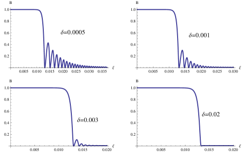
Figure 1: Profiles of MSWs [solution of Eq. (18)] are shown for different values of the viscosity parameter $\delta$ as in the figure. The other parameter values are $n_{0}=4.0\times 10^{32}m^{-3}$, $B_{0}=5.0\times 10^{3}$ T, $T_{e}=5.0\times 10^{3}$ K, $T_{i}=0.1\times T_{e}$, $\gamma=0.001$ and $M=1.5$.

$$\frac{\beta}{\alpha}\sim\frac{m_{e}}{m_{i}}\frac{V_{Fe}^{2}}{c^{2}}\ll 1;~{}\frac{\varepsilon^{2}/v_{B}^{2}}{c_{s}^{2}}\sim\left(\frac{\mu_{B}B_{0}}{k_{B}T_{e}}\right)^{2}\left(\frac{m_{i}C_{A}^{2}}{k_{B}T_{e}}\right)^{2},$$ (20)

$$\frac{\varepsilon^{2}/v_{B}^{2}}{\alpha} \sim 0.1\left(\frac{\mu_{B}B_{0}}{k_{B}T_{e}}\right)^{2}\frac{m_{i}C_{A}^{2}}{k_{B}T_{e}}\frac{m_{i}}{m_{e}}\frac{C_{A}^{2}}{H^{2}V_{Fe}^{2}}$$ (21)

$$>0.1\left(\frac{\mu_{B}B_{0}}{k_{B}T_{e}}\right)^{2}\left(\frac{m_{i}C_{A}^{2}}{k_{B}T_{e}}\right)^{2}$$

$$\sim 0.1\frac{\varepsilon^{2}/v_{B}^{2}}{c_{s}^{2}},i.e.,\alpha\gg c_{s}^{2}.$$

Thus, from Eqs. (LABEL:estimation1) and (21) it follows that the contributions from the pressure gradient and the spin forces may be comparable, however, the contribution from the exchange-correlation force is much higher than the other quantum forces. The inclusion of such force in the QMHD model, which was neglected in the previous works (e.g., Ref. sahu2015, ), is one of the main purposes of the present study. Furthermore, the source of dissipation is not only the magnetic diffusivity, but also the ion kinematic viscosity which gives an additional term in Eq. (18) that was also omitted in the previous studies sahu2015 . For typical astrophysical plasmas with $n_{0}=4\times 10^{32}$ m^-3, $T_{e}=0.1T_{i}=5\times 10^{3}$ K and $B_{0}=5\times 10^{3}$ T, we have $\alpha\sim 6\times 10^{3},~{}\beta\sim 10^{-3},~{}\varepsilon^{2}/v_{B}^{2}\sim 0.3$ and $c_{s}^{2}\sim 1.5$. Decreasing only the value of $T_{e}~{}(\sim 10^{3}$ K) results into a higher value of $\varepsilon^{2}/v_{B}^{2}~{}(\sim 40)$ than $c_{s}^{2}\sim 0.3$. However, slightly decreasing the magnetic field ($B_{0}=4\times 10^{3}$ T) or increasing the number density ($n_{0}=7\times 10^{32}$ m^-3) gives $\alpha\sim 9\times 10^{3},~{}\beta\sim 10^{-3},~{}\varepsilon^{2}/v_{B}^{2}\sim 0.2$ and $c_{s}^{2}\sim 3$, i.e., higher values of $\alpha$ and $c_{s}^{2}$ without any significant change in $\beta$ and $\varepsilon^{2}/v_{B}^{2}$.

In what follows, we numerically solve Eqs. (18) and (19), and study the influence of the plasma parameters on the large amplitude MSWs. To this end we use MATHEMATICA and apply the finite difference scheme. For a fixed value of the plasma resistivity, the effects of the parameter $\delta$ associated with the kinematic viscosity on the shock profiles are shown in Fig. 1. It is seen that a transition from oscillatory to monotonic shocks occurs with increasing values of $\delta$. The corresponding phase portraits are exhibited in Fig. 2. For very low values of $\delta$, we have a train of oscillations (few of which corresponds to solitons) and the corresponding phase-space trajectory clearly shows a stable closed periodic orbit. As the value of $\delta$ increases, the dissipative effect becomes stronger and the oscillatory shocks tend to become more and more monotonic. When the dissipative effect is large enough, we have a completely monotonic shock profile without any oscillation. It is also found that kinematic viscosity has no effect on the amplitude of the shock structures. Thus numerical investigations show the existence of both oscillatory shock for weak dissipation and monotonic shock for strong dissipation. Similar features are also observed (not shown in the figure) by increasing the parameter $\gamma$ associated with the magnetic diffusivity (plasma resistivity) and keeping $\delta$ fixed. However, in this case, the number of oscillations in front of the shock becomes less in number and the heights of oscillations get reduced.

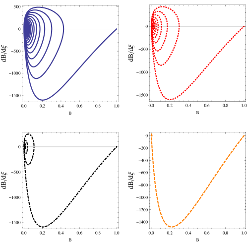
Figure 2: The phase portraits [solution of Eq. (18)] are shown for different values of $\delta$ as in Fig. 1. The solid, dotted, dash-dotted and dashed lines [from left to right (upper to lower) panels], respectively, correspond to $\delta=0.0005,~{}0.003,~{}0.001$ and $0.02$. The other parameters are the same as in Fig. 1.

Figure 3 shows the profiles of MSWs by the effects of the exchange-correlation parameter $\alpha$. It is observed that as the value of $\alpha$ (or the quantum parameter $H$) decreases, i.e., as one enters into the high-density regimes, the dissipative effects prevail over that of the quantum particle dispersion, and the oscillations in front of the shock decrease in number, resulting into the monotonic shock transition. From the parameter estimation as above, it is also evident that the exchange-correlation force plays a dominating role of dispersion over the other quantum and pressure gradient forces. The individual effects of different quantum forces on the shock profiles can also be stated. If one drops (retains) the term $\propto$ $\beta$ (however, retains or drops those with $c_{s}$, $\varepsilon$) and retains the values of $\alpha$, $\gamma$ and $\delta$ as in the upper left panel of Fig. 3, then only monotonic (oscillatory) shocks can be seen, i.e., the dispersion from the exchange-correlation force is not sufficient to prevail over the dissipation. From the numerical simulation, we also find that the shock strength decreases with increasing values of $\beta$, however, the same increases (decreases) with increasing (decreasing) values of the Zeeman energy $\varepsilon$. Thus, we conclude that in a spin QMHD model, one must take into account the effects of the exchange-correlation force of fermions along with the quantum force associated with the Bohm potential in order to get more physical insights in the propagation of MSWs in quantum magneto-plasmas.

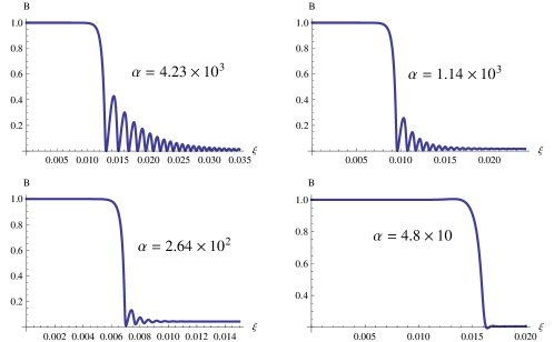
Figure 3: Profiles of nonlinear solutions of Eq. (18) for different values of exchange correlation parameter $\alpha$ ($\alpha=4.23\times 10^{3}$ and $H=0.19$ for $n_{0}=4.0\times 10^{32}$, $\alpha=1.14\times 10^{3}$ and $H=0.22$ for $n_{0}=1.5\times 10^{32}$, $\alpha=2.64\times 10^{2}$ and $H=0.27$ for $n_{0}=5.0\times 10^{31}$, $\alpha=4.8\times 10^{1}$ and $H=0.33$ for $n_{0}=1.4\times 10^{31}$), where $\delta=0.0005$, and the other parameters are same as in Fig. 1.

V Conclusion

We have presented a theoretical study on the multidimensional propagation of arbitrary amplitude quantum magnetosonic shocks in a spin-$1/2$ quantum dissipative plasma with the effects of quantum force (Bohm potential), the pressure-like spin force as well as the exchange and correlation force of electrons. The effects of ion kinematic viscosity and the plasma resistivity are also considered to account for the dissipation in the QMHD model. It is found that the contribution from the exchange-correlation force is dominant over all other similar forces and it plays a significant role on transition from monotonic to oscillatory shocks. The numerical solution confirms the existence of both oscillatory and monotonic shock profiles (depending on the strengths of the dissipation and dispersion effects). It is seen that as the ion viscosity or the magnetic diffusivity parameter increases, the oscillatory shock structure becomes more and more monotonic. Also, both the oscillatory and monotonic shocks depend not only on the dissipative parameters but also on the quantum force (diffraction) or the exchange-correlation force. It is observed that an oscillatory shock profile transforms into a monotonic one when the value of the quantum diffraction parameter $(\beta)$ (or the particle number density $n_{0}$) increases or that due to the exchange-correlation force $(\alpha)$ decreases.

To conclude, the results should be useful for understanding the nonlinear propagation of large amplitude magnetosonic shock-like perturbations that may be generated in many astrophysical plasma environments such those in the interior of magnetic white dwarf stars, neutron stars etc. where plasma spins up either by means of the plasma viscosity or the interior magnetic field easson1979 .

- (1) A. Markowich, C. Ringhofer, and C. Schmeiser, Semiconductor Equations (Vienna, Springer, 1990).
- (2) M. Opher, L. O. Silva, D. E. Dauger, V. K. Decyk, and J. M. Dawson, Phys. Plasmas 8, 2454 (2001); G. Chabrier, F. Douchin, and A. Y. Potekhin, J. Phys. Condens. Matter 14, 9133 (2002).
- (3) M. Opher, L. O. Silva, D. E. Danger, V. K. Decyk, and J. M. Dawson, Phys. Plasmas 8, 2454 (2001).
- (4) G. Chabrier, F. Douchin, and A. Y. Potekhin, J. Phys.: Condens. Matter 14, 9133 (2002).
- (5) H. Haug and S. W. Koch, Quantum Theory of the Optical and Electronic Properties of Semiconductors (World Scientific, London, 2004).
- (6) W. Li, P. J. Tanner, and T. F. Gallagher, Phys. Rev. Lett. 94, 173001 (2005).
- (7) L. K. Ang and P. Zhang, Phys. Rev. Lett. 98, 164802 (2007).
- (8) M. Leontovich, Izv. Akad. Nauk Arm. SSR, Fiz. 8, 16 (1994).
- (9) M. Murklund and P. K. Shukla, Rev. Mod. Phys. 78, 591 (2006).
- (10) S. H. Glenzer, G. Gregori, R. W. Lee, F. J. Rogers, S. W. Pollaine, and O. L. Landen, Phys. Rev. Lett. 90, 175002 (2003).
- (11) S. H. Glenzer and R. Redmer, Rev. Mod. Phys. 81, 1625 (2009).
- (12) G. Manfredi, Fields Inst. Commun. 46, 263 (2005).
- (13) C. L. Gardner and C. Ringhofer, Phys. Rev. E 53, 157 (1996).
- (14) G. Manfredi and F. Haas, Phys. Rev. B 64, 075316 (2001).
- (15) F. Haas, Phys. Plasmas 12, 062117 (2005).
- (16) M. W. Walser and C. H. Keitel, J. Phys. B 33, L221 (2000).
- (17) Z. Qian and Vignale, Phys. Rev. Lett. 88, 056404 (2002).
- (18) R. L. Liboff, Europhys. Lett. 68, 577 (2004).
- (19) L. Brey, J. Dempsey, N. F. Johnson, and B. Halperin, Phys. Rev. B 42, 1240 (1990).
- (20) G. Manfredi and F. Haas, Phys. Rev. B 64, 075316 (2001).
- (21) N. Crouseilles, P. A. Hervieux, and G. Manfredi, Phys. Rev. B 78, 155412 (2008).
- (22) G. Brodin, A. P. Misra, and M. Marklund, Phys. Rev. Lett. 105, 105004 (2010).
- (23) P. K. Shukla and B. Eliasson, Phys. Rev. Lett. 108, 165007 (2012).
- (24) P. K. Shukla, Nat. Phys. 5, 92 (2009).
- (25) M. Marklund and G. Brodin, Phys. Rev. Lett. 98, 025001 (2007).
- (26) G. Brodin and M. Marklund, New J. Phys. 9, 277 (2007).
- (27) G. Brodin and M. Marklund, Phys. Rev. E 76, 055403 (R) (2007).
- (28) M. Marklund, B. Eliasson, P.K. Shukla, Phys. Rev. E 76, 067401 (2007).
- (29) A. P. Misra and N. K. Ghosh, Phys. Lett. A 372, 6412 (2008).
- (30) A. Mushtaq and S. V. Vladimirov, Eur. Phys. J. D 64, 419 (2011).
- (31) B. Sahu, S. Choudhury, and A. Sinha, Phys. Plasmas 22, 022304 (2015).
- (32) A. P. Misra, G. Brodin, M. Marklund, and P. K. Shukla, Phys. Rev. E 82, 056406(͑2010); Phys. Plasmas 17, 122306 (2010).
- (33) L. Hedin and B. I. Lundqvist, J. Phys. C: Solid State Phys. 4, 2064 (1971).
- (34) P. K. Shukla and A. A. Mamun, New J. Phys. 5, 17 (2003).
- (35) I. Easson, Astrophys. J. 228, 257 (1979).