ac properties of short Josephson weak links

Abstract

We calculate the admittance of two types of Josephson weak links—the first is a one-dimensional superconducting wire with a local suppression of the order parameter, and the second is a short S-c-S structure, where S denotes a superconducting reservoir and c is a constriction. The systems of the first type are analyzed on the basis of time-dependent Ginzburg-Landau equations derived by Gor’kov and Eliashberg for gapless superconductors with paramagnetic impurities. It is shown that the impedance $Z(\Omega)$ has a maximum as a function of the frequency $\Omega$, and the electric field $E_{\Omega}$ is determined by two gauge-invariant quantities. One of them is the condensate momentum $Q_{\Omega}$ and another is a potential $\mu$ related to charge imbalance. The structures of the second type are studied on the basis of microscopic equations for quasiclassical Green’s functions in the Keldysh technique. For short S-c-S contacts (the Thouless energy ${E_{\text{Th}}=D/L^{2}\gg\Delta}$) we present a formula for admittance $Y$ valid frequencies $\Omega$ and temperatures $T$ less than the Thouless energy $E_{\text{Th}}$ (${\hbar\Omega,T\ll E_{\text{Th}}}$) but arbitrary with respect to the energy gap $\Delta$. It is shown that, at low temperatures, the absorption is absent [${\mathrm{Re}(Y)=0}$] if the frequency does not exceed the energy gap in the center of the constriction (${\Omega<\Delta\cos\varphi_{0}}$, where $2\varphi_{0}$ is the phase difference between the S reservoirs). The absorption gradually increases with increasing the difference ${(\Omega-\Delta\cos\varphi_{0})}$ if $2\varphi_{0}$ is less than the phase difference $2\varphi_{\text{c}}$ corresponding to the critical Josephson current. In the interval ${2\varphi_{\text{c}}<2\varphi_{0}<\pi}$, the absorption has a maximum. This interval of the phase difference is achievable in phase-biased Josephson junctions. Close to $T_{\text{c}}$ the admittance has a maximum at low $\Omega$ which is described by an analytical formula.

I Introduction

The study of dynamic effects in superconductors began soon after the appearance of microscopic BCS theory of superconductivity.Bardeen et al. (1957) Using the BCS theory, Mattis and Bardeen have calculated the admittance of a superconductor $Y(\Omega,q)$.Mattis and Bardeen (1958) Later, Abrikosov, Gor’kov and Khalatnikov have obtained the admittance for pure superconductors by using the Green’s function technique.Abrikosov et al. (1958) This technique was applied by Abrikosov and Gor’kov to calculate the linear response of superconductors with impurities.Abrikosov and Gor’kov (1959) In more detail, the theory of admittance has been later developed by Nam.Nam (1967a); *Nam67_a In these papers, it has been shown that at low temperatures absorption is absent if the frequency of electromagnetic field $\Omega$ is less than $2\Delta$. This means that the real part of admittance ${\mathrm{Re}[Y(\Omega)]\equiv Y^{\prime}(\Omega)}$ equals zero in the limit ${T\to 0}$ and ${\Omega<2\Delta/\hbar}$. If frequency $\Omega$ exceeds $2\Delta$, $Y^{\prime}(\Omega)$ increases with increasing the difference ${(\Omega-2\Delta)}$.

On the other hand, the intensive study of dynamic collective modes in superconductors, both in low- and high-T${}_{\text{c}}$ ones, is carried out in the last decade. A special attention is paid to the amplitude mode (AM), which is called often in literature the Higgs mode.Higgs (1964) This mode has been studied theoretically long agoVolkov and Kogan (1974); Kulik et al. (1981); Barankov et al. (2004); *Levitov04a; Amin et al. (2004); Warner and Leggett (2005); Szymańska et al. (2005); Yuzbashyan et al. (2005); *Altshuler05a; Yuzbashyan and Dzero (2006); Yuzbashyan (2008); Gurarie (2009); Krull et al. (2014); Moor et al. (2014); Dzero et al. (2015); Yuzbashyan et al. (2015); Peronaci et al. (2015); Kemper et al. (2015); Tsuji and Aoki (2015); Cea et al. (2015, 2016); Murakami et al. (2016); Sentef et al. (2016); Chou et al. (2016); Yoon and Watanabe (2015), but only recently it was observed in experiments.Matsunaga et al. (2013, 2014) A superconductor (Nb_1-xTi_xN) was driven out of the equilibrium by a short laser pulse (teraherz frequency range) and the temporal evolution of the deviation $\delta\Delta(t)$ from the equilibrium value $\Delta$ was detected by a weak probe signal in picosecond time interval. This evolution can be qualitatively described by the equationVolkov and Kogan (1974)

$$\delta\Delta(t)\propto\delta\Delta(0)\frac{\cos(2\Delta t/\hbar)}{\sqrt{2\Delta t/\hbar}}\,.$$ (1)

A weak incident electric field ${\mathbf{E}(t)=\mathbf{E}_{\Omega}\cos(\Omega t)}$ obviously can not lead to a perturbation of the order parameter $\Delta$ because it is a scalar so that $\delta\Delta(t)$ can be proportional only to even orders of $\mathbf{E}^{2n}(t)$. However, as we have shown recently, Moor et al. (2017) the situation changes in the presence of the condensate flow. In this case, even a weak ac field $\mathbf{E}(t)$ leads to a perturbation of $\Delta$, ${\delta\Delta_{\Omega}\propto\mathbf{Q}_{\Omega}\mathbf{Q}_{0}}$, where ${\mathbf{Q}_{0}=m\mathbf{v}_{0}}$ is the condensate momentum, $\mathbf{v}_{0}$ is the velocity of the condensate, and $\mathbf{Q}_{\Omega}$ is the ac condensate momentum induced by the electric field $\mathbf{E}_{\Omega}$ according to the expression

$$-i\Omega\hbar\mathbf{Q}_{\Omega}=e\mathbf{E}_{\Omega}\,.$$ (2)

If the frequency of the external electric field $\Omega$ coincides with the frequency of the AM $2\Delta/\hbar$, a resonance absorption of the incident electromagnetic field $\mathbf{E}_{\Omega}$ takes place and the real part ${Y^{\prime}(\Omega)\equiv\mathrm{Re}[Y(\Omega)]}$ of admittance has a sharp peak at ${\Omega=2\Delta/\hbar}$.

A similar peak was obtained in Ref. Dai and Lee, 2017, where linear response of a superconductor with a finite-momentum pairing was calculated. As the authors of Ref. Dai and Lee, 2017 claim, their results can be applied to high-$T_{\text{c}}$ superconductors with a pair density wave or to superconductors in the Fulde-Ferrell-Larkin-Ovchinnikov (FFLO) state. Fulde and Ferrell (1964); Larkin and Ovchinnikov (1965) In both cases, the superconducting order parameter depends on coordinate, $\Delta(\mathbf{r})$, turning to zero at some points or lines.

High frequency properties of superconductors are important not only from the point of view of fundamental physics, but also of applications. In particular, the use of superconducting devices in qubits and in highly sensitive detectors requires the knowledge of the admittance $Y(\Omega)$.Gol’tsman et al. (2001); Day et al. (2003); Janssen et al. (2013); Clarke and Wilhelm (2008) The systems used in practical devices often include Josephson junctions (JJ), for example, S-c-S or S-n-S weak links of different types, where c denotes a constriction and n stands for a normal metal. The study of ac properties of JJs has began long ago (see references in Refs. Likharev, 1979; Barone and Patern, 1982). The admittance $Y(\Omega)$ of a short JJ of the S-c-S type has been calculated by Artemenko et al. on the basis of Keldysh technique for quasiclassical Green’s functions.Artemenko et al. (1979) It was assumed that the Thouless energy ${E_{\text{Th}}=D/L^{2}}$ is much larger than $T_{\text{c}}$. In particular, it was shown that at low frequencies $\Omega$ and close to the critical temperature $T_{\text{c}}$ the admittance has the form [see Eq. (31) in Ref. Artemenko et al., 1979]

$$Y(\Omega)=\frac{2eI_{\text{c}}(\nu_{\text{in}}+i\Omega)}{\hbar(\Omega^{2}+\nu_{\text{in}}^{2})}P(2\varphi_{0})+\frac{1}{R}\,,$$ (3)

where ${I_{\text{c}}=\pi\Delta^{2}/(4eTR)}$ is the critical current of this JJ near T${}_{\text{c}}$, $R$ is the resistance in the normal state and $\nu_{\text{in}}$ is inelastic scattering time.Kulik and Omel’yanchuk (1978) The function $P(2\varphi_{0})$ is a function of the phase difference $2\varphi_{0}$. The form of $P(\varphi_{0})$ is displayed in Fig. 5. Equation (3) shows that the reactive part of admittance has a sharp peak at a small frequency ${\Omega\simeq\nu_{\text{in}}}$ since ${\nu_{\text{in}}\ll\Delta}$.

An anomalous behavior of the admittance $Y(\Omega)$ was obtained also in Ref. Kos et al., 2013 where also a short JJ was studied by another method (tunnel Hamiltonian method and subsequent averaging via the Dorokhov’s procedure).Dorokhov (1984)

Lempitski analyzed non-stationary behavior of long (${E_{\text{Th}}\ll\Delta}$) S-n-S junctions and has shown that, in this case, inelastic scattering rate also plays an essential role.Lempitskii (1983) Such ac properties of S-n-S JJs as fluctuations of voltage and impedance at currents less than the critical one were analyzed in Ref. Nagaev, 1988. The admittance of long S-n-S junctions in the frequency range ${\Omega\ll E_{\text{Th}}/\hbar}$ has been calculated in recent papers,Virtanen et al. (2011); Tikhonov and Feigel’man (2015) where an expression for $Y(\Omega)$ similar to Eq. (3) has been obtained. This equation shows an anomalous behavior of the admittance at low frequencies where the maximal value of the admittance is determined by the energy relaxation rate $\nu_{\text{in}}$.

In the current paper, we calculate and analyze the admittance of short JJs of two configurations. In Section II, we present basic equations for quasiclassical Green’s functions which will be used in Section III, where we consider a superconducting wire or film in which the superconducting order parameter $\Psi$ is suppressed locally so that the amplitude $|\Psi(x)|$ has a dip at ${x=0}$. At strong suppression, one can speak of a weak link. This model has much in common with the so-called phase-slip centersIvlev and Kopnin (1984); Arutyunov et al. (2008) or FFLO state in superconductors.Fulde and Ferrell (1964); Larkin and Ovchinnikov (1965) Far away from the weak point ${x=0}$, the ac condensate momentum $Q_{\Omega}$ is connected with an ac field $E_{\Omega}$ via Eq. (2). Near this point, the momentum $Q_{\Omega}$ depends on coordinate, $Q_{\Omega}(x)$, and the gauge-invariant potential $\mu_{\Omega}(x)$ related to electron-hole branch imbalance arises.Tinkham and Clarke (1972); Tinkham (1972); Schmid and Schön ; Artemenko and Volkov (1979) In this case, the electric field is determined both by the gauge-invariant vector $\mathbf{Q}$ and by the gradient of the potential $\nabla\mu_{\Omega}(x)$ (see, for example, Refs. G. and Gurevich, 1974; Artemenko and Volkov, 1979),

$$\hbar\frac{\partial\mathbf{Q}}{\partial t}=e\mathbf{E}+\nabla\mu\,.$$ (4)

The gauge-invariant quantities $\mathbf{Q}$ and $\mu$ are defined in terms of the vector potential $\mathbf{A}$ and scalar electric potential $V$

$$\mathbf{Q} =\frac{1}{2}(\nabla\chi-2\pi\mathbf{A}/\Phi_{0})\,,$$ (5)

$$\mu =\frac{1}{2}(\hbar\frac{\partial\chi}{\partial t}+2eV)\,,$$ (6)

where $\chi$ is the phase of the order parameter and ${\Phi_{0}=hc/2e}$ is the magnetic flux quantum. Substituting Eqs. (5) and (6) into Eq. (4), we obtain the standard definition of the electric field $\mathbf{E}$ in terms of potentials $\mathbf{A}$ and $V$, ${\mathbf{E}=-(1/c)\partial_{t}\mathbf{A}-\nabla V}$.

On the basis of time-dependent Ginzburg-Landau equations derived by Gor’kov and Eliashberg for gapless superconductors,Gor’kov and Eliashberg (1968) we find both quantities $Q_{\Omega}(x)$ and $\mu_{\Omega}(x)$, and calculate the admittance of the system. We will show that the last term at the right is comparable with the first one and therefore can not be neglected as it was done in some papers.

In Section IV we consider a short S-c-S contact. By using a rather general formula for admittance derived in Ref. Artemenko et al., 1979, we analyze the admittance of this JJ. [The authors of Ref. Artemenko et al., 1979 provided the expression Eq. (3) without considering arbitrary frequencies and temperatures.] In this case, the electric field $E_{\Omega}$ is connected with the phase difference $\varphi_{\Omega}$ in superconducting reservoirs S which are assumed to be in equilibrium. We present the dependence $Y(\Omega)$ for different values of constant phase difference $2\varphi_{0}$ and arbitrary frequencies. We show that an interesting peculiarity in this dependence arises near the point ${\varphi_{0}\simeq\pi/4}$ corresponding to the critical current $I_{\text{c}}$. Whereas the real part of admittance ${Y^{\prime}(\Omega)=\mathrm{Re}[Y(\Omega)]}$ increases smoothly with increasing $\Omega$ at ${2\varphi_{0}<\pi/2}$, it has a maximum if the phase difference $2\varphi_{0}$ exceeds $\pi/2$. Although the latter case corresponds to unstable points on the curve $I_{\text{J}}(\varphi_{0})$ in current-biased JJs, it can be realized in phase-biased JJs making the predicted effect observable.Dassonneville et al. (2013); Ronzani et al. (2016)

In the Conclusion, we discuss the possibilities to study ac properties of the considered JJs experimentally. Note that a hump in the real part of admittance $Y^{\prime}(\Omega)$ at high temperatures and low $\Omega$ is much broader than the peak in $Y^{\prime}(\Omega)$ caused by a resonance excitation of the AM in uniform superconductors and is due to another mechanism.Moor et al. (2017)

II Basic Equations

In this Section, we present basic equations for quasiclassical Green’s functions including the Keldysh function which is needed in a non-stationary case. These equations were employed in our previous work for analysis of a uniform caseMoor et al. (2017) and will be used for calculating the admittance of a non-uniform superconductor, i.e., a short S-c-S JJ. We have shown earlier that the AM can be excited even by a weak ac field $\mathbf{E}(t)$ in the presence of a condensate flow. In addition, it was shown that the resonance excitation of the AM contributes to the admittance $Y(\Omega)$ of such a superconductor. Unlike the experiments in terahertz frequency region,Matsunaga et al. (2013, 2014) the absorption of microwave ac field in superconductors was measured long ago by Martin and TinkhamMartin and Tinkham (1968) and later on by Budzinski et al.Budzinski et al. (1973) It was found that a peak near the frequency ${\Omega=2\Delta/\hbar}$ arises by applying a magnetic field. The formula describing correctly this peak was obtained by the method of analytical continuation in Ref. Ovchinnikov and Isaakyan, 1978, the authors of which explained the maximum in the absorption with a singularity in the density of states but did not relate it with the resonance excitation of the amplitude (Higgs) mode.

Like in Ref. Moor et al., 2017, we consider the diffusive limit in one-dimensional geometry so that ${\mathbf{Q}=(Q,0,0)}$. The current $\mathbf{I}_{\Omega}$ and the gap perturbation $\delta\Delta_{\Omega}$ are found from nonstationary equations for matrix quasiclassical Green’s functions $\check{g}$. These equations, in the absence of a magnetic field, have the formUsadel (1970); Kopnin (2001); Larkin and Ovchinnikov (1986); Rammer and Smith (1986); Belzig et al. (1999); Artemenko and Volkov (1979)

$$-iD\partial_{x}(\check{g}\partial_{x}\check{g})+i(\check{\tau}_{3}\cdot\partial_{t}\check{g}+\partial_{t^{\prime}}\check{g}\cdot\check{\tau}_{3})+[\check{\Sigma}\,,\check{g}]=V(t)\check{g}-\check{g}V(t^{\prime})\,.$$ (7)

The diagonal matrix elements of the matrix $\check{g}$ are the retarded (advanced) Green’s functions $\hat{g}^{R(A)}$, and the off-diagonal element is the Keldysh function $\hat{g}$,

$$\check{g}=\begin{pmatrix}\hat{g}^{R}&\hat{g}\\ 0&\hat{g}^{A}\end{pmatrix}\,.$$ (8)

The functions $\hat{g}^{R(A)}$ and $\hat{g}$ are $2\times 2$ matrices in the particle-hole space. All the functions depend on two times $t$ and $t^{\prime}$. The diagonal matrix $\check{\Sigma}$ consists of matrices ${\hat{\Sigma}^{R(A)}=\Delta i\hat{\tau}_{2}+i\hat{\gamma}^{R(A)}}$, where $\Delta$ is the superconducting gap and $\hat{\gamma}$ is a damping matrix. The matrix $\check{g}(t,t^{\prime})$ obeys the normalization condition

$$\check{g}\cdot\check{g}\equiv\int dt_{1}\check{g}(t,t_{1})\cdot\check{g}(t_{1},t^{\prime})=\check{1}\delta(t-t^{\prime})\,.$$ (9)

The current in the diffusive limit is determined by the expression

$$\mathbf{I}(t)=-\frac{\pi\sigma}{4e}\int dt_{1}\mathrm{Tr}\big{\{}\check{\tau}_{3}\check{g}(t,t_{1})\nabla\check{g}(t_{1},t)\big{\}}^{K}\,,$$ (10)

where $\sigma$ is the conductivity.

In equilibrium and in absence of a dc current, the Green’s functions $\hat{g}^{R(A)}$ and $\hat{g}$ have the form

$$\hat{g}_{\text{eq}}^{R(A)} =[g\hat{\tau}_{3}+fi\hat{\tau}_{2}]^{R(A)}\,,$$ (11)

$$\hat{g}_{\text{eq}} =(\hat{g}^{R}-\hat{g}^{A})\tanh(\epsilon\beta)\,,$$ (12)

where ${g_{\text{eq}}^{R(A)}=(\epsilon/\Delta)f_{\text{eq}}^{R(A)}=\epsilon/\zeta^{R(A)}(\epsilon)}$, ${\beta=1/2T}$ and

$$\zeta^{R(A)}(\epsilon)=\sqrt{(\epsilon\pm i\gamma)^{2}-\Delta^{2}}\,.$$ (13)

The matrices $\hat{\tau}_{i}$ are the Pauli matrices operating in the particle-hole space.

We calculate the impedance and the gauge-invariant quantities $Q$ and $\mu$ in the next Section where nonstationary Ginzburg-Landau equationsGor’kov and Eliashberg (1968) will be used instead of more complicated Eqs. (7)–(9).

III Superconducting wire with a local gap suppression

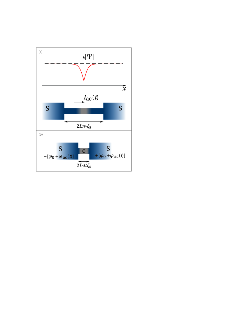
Figure 1: (Color online.) Schematic view of the system under consideration. (a) The general suppression of the order parameter in a junction and a general setup of a weak link of the length ${2L\gg\xi_{\text{s}}}$; (b) a short weak link (${2L\ll\xi_{\text{s}}}$) with corresponding phases of the order parameters in the superconductors forming the junction.

We consider a one-dimensional superconducting wire or film in which the superconducting order parameter ${\Delta\propto\Psi}$ is locally suppressed, see Fig. 1 (a). Our aim is to calculate the impedance (or admittance) of this system. We describe the system under consideration on the basis of non-stationary Ginzburg-Landau equations that have been derived by Gor’kov and EliashbergGor’kov and Eliashberg (1968) and were used in many papers. These equations are valid for gapless superconductors with a high concentration of paramagnetic impurities. In the normalized form they have the form

$$\partial_{t}f =\partial_{xx}^{2}f+f[a(x)-f^{2}]-Q^{2}f\,,$$ (14)

$$\nu f^{2}\mu =-\partial_{x}E\,,$$ (15)

$$I =Qf^{2}+E\,,$$ (16)

$$\partial_{t}Q =E+\partial_{x}\mu\,.$$ (17)

Here, ${f=|\Psi|/|\Psi_{\infty}|}$ is the dimensionless modulus of the order parameter $\Psi$, where ${|\Psi_{\infty}|=\pi\sqrt{(T_{\text{c}}^{2}-T^{2})}}$. The length and time are measured in the units ${\xi_{\text{sf}}=\sqrt{12Dt_{0}}}$ and ${t_{0}=\hbar^{2}/(2\tau_{\text{sf}}\Delta^{2})}$, where $\tau_{\text{sf}}$ is the spin-flip relaxation time. The current $I$ and the voltage $V$ are measured in units of $\sigma V_{0}/\xi_{\text{sf}}$ and ${V_{0}=\hbar/2et_{0}}$. The gauge-invariant quantities $\mathbf{Q}$ and $\mu$ are defined in Eqs. (5) and (6).

The magnitude of the relaxation rate $\nu$ of the normalized potential $\mu$ depends on the choice of the model. In the model of a gapless superconductor with paramagnetic impurities considered in Ref. Gor’kov and Eliashberg, 1968 ${\nu=12}$. The value of $\nu$ in conventional BCS superconductors is much smaller.Artemenko and Volkov (1979) The coefficient $a(x)$ describes a suppression of $|\Psi|$, respectively, $f$. We consider the simplest model when $a(x)$ has the form

$$a(x)=1-a_{0}\delta(x)\,,$$ (18)

where the parameter $a_{0}$ can be either small (weak suppression of $f$) or large (strong suppression of $f$). The reasons for the suppression of $\Delta$ can be different. For example, a locally enhanced concentration of paramagnetic impurities leads to such a suppression. Note that the stationary and non-stationary Josephson effects for large $a_{0}$ have been studied in Ref. Volkov, 1971; *Volkov74.

From Eq. (18) we find the matching condition

$$2\partial_{x}f(x)|_{x=0}=a_{0}f(0)\,.$$ (19)

In this Section, we consider the case when only ac current flows through the system. From Eqs. (14)–(18), one needs to find a spatial dependence $f_{0}(x)$ in a stationary case and then to determine the linear response to the ac current $I_{\text{ac}}(t)$ in the system. Consider first the stationary case.

III.1 Stationary case

In absence of a constant current (${I_{0}=0}$) we need to find a stationary solution only for Eq. (14) complemented by the boundary condition Eq. (19) because the functions $Q_{0}$, $\mu$ and $E$ vanish. The solution is

$$f_{0}(x)=\tanh X$$ (20)

with ${X=\kappa_{0}(|x|+x_{0})}$ and ${\kappa_{0}^{2}=1/2}$. The integration constant ${X_{0}\equiv\kappa_{0}x_{0}}$ is found from the matching condition Eq. (19),

$$\sinh(2X_{0})=\frac{4\kappa_{0}}{a_{0}}\,.$$ (21)

In the case of weak (${a_{0}\ll 1}$), respectively, strong (${a_{0}\gg 1}$) suppression, the constant ${X_{0}=\kappa_{0}x_{0}}$ is

$$X_{0}=\begin{cases}2^{-1}\ln(8\kappa_{0}/a_{0})\,,&a_{0}\ll 1\,,\\ 2\kappa_{0}/a_{0}\,,&a_{0}\gg 1\,.\end{cases}$$ (22)

The dependence $f_{0}(x)$ is shown schematically in Fig. 1 (a).

Next, we consider the non-stationary case.

III.2 Non-stationary case

Having determined the stationary function $f_{0}(x)$, we can find the linear response, i.e., the functions $Q_{\Omega}$, $\mu_{\Omega}$ and $E_{\Omega}$ in the presence of a weak ac current

$$I_{\text{ac}}(t)=I_{\Omega}\cos(\Omega t)\,.$$ (23)

We can linearize Eqs. (14)–(17). Far away from the point ${x=0}$, where the normalized order parameter ${f(x)\to 1}$, we obtain

$$E_{\infty}=\frac{-i\Omega}{1-i\Omega}I_{\Omega}\,,$$ (24)

$$Q_{\infty}=\frac{1}{1-i\Omega}I_{\Omega}\,.$$ (25)

Deviations from these values, ${\delta E_{\Omega}=E_{\Omega}-E_{\infty}}$ and ${\delta Q_{\Omega}=Q_{\Omega}-Q_{\infty}}$, arise due to a local suppression of superconductivity at ${x=0}$. We introduce a function $\mathcal{E}_{\Omega}(x)$ which is connected with $\delta E_{\Omega}(x)$ via the relation ${\delta E_{\Omega}=f_{0}(x)\mathcal{E}_{\Omega}}$. The function $\mathcal{E}_{\Omega}$ obeys the equation (see Appendix A)

$$\Big{[}-\partial_{xx}^{2}+\nu(\tanh^{2}X-i\Omega)+\frac{1}{\sinh^{2}X}\Big{]}\mathcal{E}_{\Omega}=\frac{-2iI_{\Omega}\Omega\nu}{(1-i\Omega)\sinh(2X)}\,.$$ (26)

The boundary condition at ${x=0}$ for the function $\mathcal{E}_{\Omega}$ is

$$2\partial_{x}\mathcal{E}_{\Omega}|_{0+}=-a_{0}\mathcal{E}_{\Omega}(0)\,.$$ (27)

We need to solve Eq. (26) and to find an even function $\mathcal{E}_{\Omega}(x)$ decaying to zero at ${x\to\infty}$. The ac voltage $\delta V_{\Omega}$ across the junction is expressed through $\mathcal{E}_{\Omega}$ via

$$\delta V_{\Omega}=2\int_{0}^{\infty}dx\,f_{0}(x)\mathcal{E}_{\Omega}(x)\,.$$ (28)

The complex impedance of the system consists of two parts ${Z_{\Omega}=Z_{\Omega L}+\delta Z_{\Omega}}$, where the first term is the impedance in the absence of the weak link (${a_{0}=0}$) and the second term is related to the presence of the local suppression

$$Z_{\Omega L} =\frac{-i\Omega}{1-i\Omega}2L\,,$$ (29)

$$\delta Z_{\Omega} =\frac{\delta V_{\Omega}}{I_{\Omega}}\,.$$ (30)

Note that for small $a_{0}$ the problem can be solved analytically. Consider first this case.

III.2.1 Weak local suppression

As follows from Eq. (21), for small $a_{0}$ we have ${\sinh X\simeq\exp[(|x|+x_{0})/\sqrt{2}]\gg 1}$. In the main approximation, Eq. (26) can be written in the form

$$-\partial_{xx}^{2}\mathcal{E}_{\Omega}+\mathcal{E}_{\Omega}\kappa_{\Omega}^{2}=-4i\Omega I_{\Omega}\frac{\nu\exp[-\sqrt{2}(|x|+x_{0})]}{1-i\Omega}\,,$$ (31)

where ${\kappa_{\Omega}^{2}=\nu(1-i\Omega)}$. In the case of a small parameter $a_{0}$, a solution with continuous functions $\mathcal{E}_{\Omega}(x)$ and $\partial_{x}\mathcal{E}_{\Omega}(x)$ is

$$\mathcal{E}_{\Omega}(x) =\frac{-4ia_{0}\Omega\nu I_{\Omega}}{(1-i\Omega)(\kappa_{\Omega}^{2}-2)}$$ (32)

$$\times\Big{[}-\frac{\sqrt{2}}{\kappa_{\Omega}}\exp(-\kappa_{\Omega}|x|)+\exp(-\sqrt{2}|x|)\Big{]}\exp(-\sqrt{2}|x_{0}|)\,.$$

For the voltage $\delta V_{\Omega}$ and the impedance $\delta Z_{\Omega}$ we obtain

$$\delta V_{\Omega} =a_{0}\frac{-i\Omega I_{\Omega}}{(1-i\Omega)^{2}}$$ (33)

and

$$\delta Z_{\Omega} =a_{0}\frac{-i\Omega}{(1-i\Omega)^{2}}\,,$$ (34)

respectively. Therefore, the impedance variation ${\delta Z_{\Omega}=\delta Z_{\Omega}^{\prime}+i\delta Z_{\Omega}^{\prime\prime}}$ is given by

$$\delta Z_{\Omega}^{\prime}\equiv\delta R(\Omega) =a_{0}\frac{2\Omega^{2}}{(1+\Omega^{2})^{2}}\,,$$ (35)

$$\delta Z_{\Omega}^{\prime\prime} =-a_{0}\frac{\Omega(1-\Omega^{2})}{(1+\Omega^{2})^{2}}\,.$$ (36)

The total resistance and the reactive part of the impedance of the wire is

$$R(\Omega)\equiv Z^{\prime}(\Omega) =\frac{\Omega^{2}}{(1+\Omega^{2})}\Big{[}2L+\frac{2a_{0}}{(1+\Omega^{2})}\Big{]}\,,$$ (37)

$$Z^{\prime\prime}(\Omega) =-\frac{\Omega}{(1+\Omega^{2})}\Big{[}2L+\frac{a_{0}(1-\Omega^{2})}{(1+\Omega^{2})}\Big{]}\,.$$ (38)

One can see that the active part of the impedance increases due to a suppression of the order parameter $f$ at ${x=0}$. The reactive part increases at ${\Omega\leq 1}$ and decreases at ${\Omega\geq 1}$, that is, the variation of the reactive part $\delta Z_{\Omega}^{\prime\prime}$ changes sign at ${\Omega=1}$.

It is of interest to find also the admittance $Y(\Omega)\equiv 1/Z(\Omega)$. From Eqs. (30), (35), and (36) in the main approximation in the parameter $a_{0}$, we obtain

$$Y(\Omega)=\frac{1}{2L}\Big{[}1-\frac{1-a_{0}/2L}{i\Omega}\Big{]}\,.$$ (39)

This expression shows that the considered system can be modelled as a conductance and an inductance connected in parallel. The small gap suppression causes a small increase in the inductance ${\mathcal{L}=2L/(1-a_{0}/2L)}$ and does not change the real part of the conductance.

III.2.2 Strong local suppression

At strong suppression (${a_{0}\gg 1}$), the solution of Eq. (26), which looks like the “Schroedinger” equation with a complex potential, can be found numerically. In Figs. 2 (a) and 2 (b) we plot the frequency dependence of the changes in the real and imaginary parts of the impedance $\delta Z_{\Omega}^{\prime}$ and $\delta Z_{\Omega}^{\prime\prime}$ for different values of $a_{0}$. For small $a_{0}$, the results of numerical calculations and the analytical expressions given by Eqs. (35) and (36) coincide.

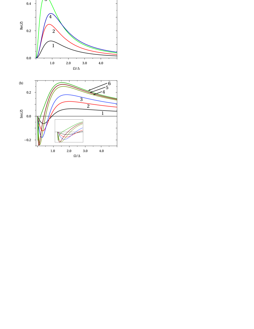
Figure 2: (Color online.) (a) Frequency dependence of the resistance variation due to a superconductivity suppression. The numbers on the curves denote, correspondingly, the values for $a_{0}$, i.e., (1) ${a_{0}=0.5}$; (2) ${a_{0}=1.0}$; (3) ${a_{0}=2.0}$; (4) ${a_{0}=5.0}$. (b) Frequency dependence of the variation of the reactive part of impedance due to a superconductivity suppression. The numbers on the curves denote, correspondingly, the values for $a_{0}$, i.e., (1) ${a_{0}=0.5}$; (2) ${a_{0}=1.0}$; (3) ${a_{0}=2.2}$; (4) ${a_{0}=2.4}$; (5) ${a_{0}=2.6}$; (6) ${a_{0}=2.8}$. The inset shows the enlarged part of $\mathrm{Im}(Z)$ at $\Omega\leq\Delta$.

We see that the resistance due to the weak link $\delta R(\Omega)$ is positive and has a broad maximum at frequencies $\Omega_{m}$ that are slightly less than $1$ (at small $a_{0}$). The position of the maximum shifts towards smaller $\Omega_{m}$ with increasing $a_{0}$ (when $a_{0}$ remains less than $\approx 2.5$). The reactive part of the impedance $\delta Z_{\Omega}^{\prime\prime}$ changes sign at approximately the same frequencies. At ${a_{0}\gtrsim 2.5}$, the maximum value of $\delta R(\Omega)$ decreases with further increase of $a_{0}$, whereas the frequency $\Omega_{m}$ increases [see Fig. 2 (a)]. The behaviour of the reactive part $\delta Z_{\Omega}^{\prime\prime}$ also changes. It is worth noting that in the considered model of a gapless superconductor, the parameter $|\Psi|$ is the amplitude of the superconducting order parameter, but not the gap.

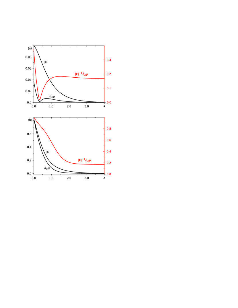
Figure 3: (Color online.) Frequency dependence of the electric field variation ${\delta E_{\Omega}(x)=f_{0}(x)\mathcal{E}_{\Omega}(x)}$ and the derivative $\partial_{x}\mu_{\Omega}(x)$ as well as their ratio for (a) ${a_{0}=0.5}$; (b) ${a_{0}=2.4}$. In both cases, the frequency ${\Omega=0.8\Delta}$. All quantities are corespondingly normalized, see Eqs. (14)–(17).

In Figs. 3 (a) and 3 (b) we display the spatial dependence of the dimensionless electric field ${\delta E_{\Omega}(x)=f_{0}(x)\mathcal{E}_{\Omega}(x)}$ and compare it to the magnitude of the spatial derivative of the gauge-invariant potential $\partial_{x}\mu_{\Omega}(x)$ for two values of $a_{0}$, i.e., for ${a_{0}=0.5}$ (weak suppression) and ${a_{0}=2.4}$ (strong suppression). One can see that these quantities may be comparable in their values. This means that the electric field $\mathbf{E}_{\Omega}$ is not determined only by the condensate momentum $\mathbf{Q}_{\Omega}$ [see Eq. (2) which is valid in a uniform case] and that in order to find the linear response of a superconductor with a non-homogeneous order parameter $f(x)$, the potential $\mu_{\Omega}(x)$ has to be calculated also alonside with $\mathbf{Q}_{\Omega}$ if the ac electric field $\mathbf{E}_{\Omega}$ is directed parallel to $x$ axis. This statement is true, for instance, for the case of the FFLO state (compare it with Ref. Dai and Lee, 2017, where the optical conductance of a non-homogeneous superconductor was calculated in the gauge with ${\mathbf{A}\neq 0}$ and ${V=0}$ so that ${\mu=0}$).

IV S-c-S contact

In this Section, we consider short Josephson junctions of the S-c-S or S-n-S types in the dirty limit, i.e., in the limit ${\tau T_{\text{c}}\ll 1}$, where $\tau$ is the momentum relaxation time. We also assume that there are no barriers at the S-c interfaces. In the considered model, two superconducting reservoirs S are connected by a narrow constriction. Since the length of the constriction $2L$ is assumed to be less than the coherence length ${\xi_{\text{S}}\simeq\sqrt{D/T_{\text{c}}}}$, that is, the Thouless energy is large (${D/L^{2}\gg T_{\text{c}}}$), it does not matter whether the constriction is normal or superconducting.

Formula for the impedance $Z(\Omega)$ in this case has been obtained by one of the authors (in collaboration with Artemenko and Zaitsev) in 1979Artemenko et al. (1979) on the basis of microscopic theory of the Josephson effects in these JJs, but it has not been analyzed in detail. Here, we reproduce the main steps of the derivation of this expression, correct typos in Ref. Artemenko et al., 1979 and analyze the admittance of the short S-c-S JJs in more detail. [The signs in Eq. (29) of Ref. Artemenko et al., 1979 should be changed in such a way that expressions in the curly brackets in Eqs. (27) and (29) coincide with each other if the functions $g^{A}(\epsilon_{-})$ in Eq. (27) are replaced by $g^{R}(\epsilon_{-})$. The imaginary unit $i$ in front of the right-hand side of Eq. (29) has to be dropped. The last term in Eq. (31) should have the form $\hbar i\omega\varphi_{\omega}/2eR$. Note that $\omega$ in Ref. Artemenko et al., 1979 corresponds to $-\Omega$.] Note that the admittance of a similar S-c-S contact has been calculated and analyzed in a recent paper,Kos et al. (2013) where another model and method of calculations were used.

The microscopic theory developed in Ref. Artemenko et al., 1979 is based on the generalized Usadel equation, Eq. (7), which describes the spatial dependence of the Green’s functions $\check{g}(x,t,t^{\prime})$ in the constriction. These functions are assumed to be continuous at the S-c and c-S interfaces (no potential barriers at these interfaces).

In the considered limit of a short junction, one can neglect all the terms in Eq. (7) except the first one and we obtain for the “anisotropic” part

$$\check{a}=-l\check{g}\partial_{x}\check{g}=\text{const}\,.$$ (40)

That is, the matrix $\check{a}$ does not depend on the coordinate $x$. The current $I$ through the considered JJ is expressed through the anisotropic part of the Keldysh function $\hat{a}$ as follows

$$I(t)=-\frac{\pi\sigma}{4e}\int dt_{1}\mathrm{Tr}\big{\{}\hat{\tau}_{3}\hat{g}\partial_{x}\hat{g}\big{\}}^{K}\,.$$ (41)

A formal solution of Eq. (40) is (for brevity we drop the temporal indices $t$ and $t^{\prime}$)

$$\check{g}(x)=\check{g}(0)\exp(-\check{a}x/l)\,.$$ (42)

As follows from Eq. (9), the matrices $\check{a}$ and $\check{g}(0)$ anticommute and ${\check{g}(0)\cdot\check{g}(0)=\check{1}}$. Thus, introducing the matrices ${\check{G}^{(\pm)}\equiv\big{[}\check{G}(L)\pm\check{G}(-L)\big{]}/2}$ and using Eq. (42), we obtain

$$\check{G}^{(+)} =\check{g}(0)\cosh(\check{a}L/l)\,,$$ (43)

$$\check{G}^{(-)} =\check{g}(0)\sinh(\check{a}L/l)\,,$$ (44)

where ${\check{G}(\pm L)\equiv\check{G}^{(\pm)}}$ are the known matrix Green’s functions in the reservoirs. From this equation we find

$$\check{a}=-\frac{l}{2L}\mathrm{arsinh}\big{[}2\check{G}^{(+)}\cdot\check{G}^{(-)}\big{]}\,.$$ (45)

In particular,

$$\hat{a}^{R(A)}=-(l/2L)\mathrm{arsinh}\big{[}2\hat{G}^{(+)}\cdot\hat{G}^{(-)}\big{]}^{R(A)}\,.$$ (46)

The matrices $[\hat{g}^{(\pm)}]^{R(A)}$ are expressed in terms of the retarded (advanced) Green’s functions in the reservoirs ${\hat{g}^{R(A)}(\pm L)\equiv\hat{G}^{R(A)}}$ that are known and have the form

$$\hat{G}^{R(A)}(\pm L)=\hat{S}(t,\pm L)\cdot\hat{G}_{0}^{R(A)}(t-t^{\prime})\cdot\hat{S}^{\dagger}(t^{\prime},\pm L)\,.$$ (47)

Here, we introduce the transformation matrix ${\hat{S}(t,\pm L)=\exp(i\hat{\tau}_{3}\varphi(t,\pm L)/2)}$ in order to take into account the presence of the phase of the superconducting order parameter in the banks ${\varphi(t,\pm L)=\pm[\varphi_{0}+\varphi_{\text{ac}}(t)]}$. The Green’s functions $\hat{G}_{0}^{R(A)}(\epsilon)$ in reservoirs in the absence of phase difference coincide with the matrices $\hat{g}_{\text{eq}}^{R(A)}$ defined in Eq. (11).

Consider first the stationary case.

IV.1 Stationary case

In the equilibrium case [${\varphi_{\text{ac}}(t)=0}$], the Keldysh function $\hat{a}$ depends only on the time difference ${(t-t^{\prime})}$ and its Fourier component is

$$\hat{a}(\epsilon)=\big{[}\hat{a}_{0}^{R}(\epsilon)-\hat{a}_{0}^{A}(\epsilon)\big{]}\tanh(\epsilon\beta)\,,$$ (48)

where ${\beta=1/2T}$. The matrices $\hat{a}^{R(A)}(\epsilon)$ are found from Eqs. (46) and (47),

$$\hat{a}_{0}^{R(A)}(\epsilon)=-\frac{l}{L}\big{[}\Delta\cos\varphi_{0}\hat{\tau}_{3}+\epsilon i\hat{\tau}_{2}\big{]}b^{R(A)}(\epsilon)$$ (49)

with

$$b^{R}(\epsilon)=\frac{i}{\tilde{\zeta}^{R}(\epsilon)}\mathrm{arsinh}\Big{[}\frac{\Delta\sin\varphi_{0}}{\zeta^{R}(\epsilon)}\Big{]}$$ (50)

and ${\tilde{\zeta}^{R}(\epsilon)=\sqrt{(\epsilon+i\gamma)^{2}-\Delta^{2}\cos^{2}\varphi_{0}}}$. The function $\zeta^{R}(\epsilon)$ is defined in Eq. (13).

In obtaining Eq. (49), we used the relation

$$\mathrm{arsinh}\Big{[}\frac{2\Delta\tilde{\zeta}^{R}(\epsilon)\sin\varphi_{0}}{[\zeta^{R}(\epsilon)]^{2}}\Big{]}=2\mathrm{arsinh}\Big{[}\frac{\Delta\sin\varphi_{0}}{\zeta^{R}(\epsilon)}\Big{]}\,,$$ (51)

and the expressions for $\big{\{}\hat{G}^{(+)}\big{\}}^{R(A)}$ and $\big{\{}\hat{G}^{(-)}\big{\}}^{R(A)}$, which directly follow from Eq. (47),

$$\big{\{}\hat{G}^{(+)}\big{\}}^{R(A)} =\big{\{}G(\epsilon)\hat{\tau}_{3}+F(\epsilon)i\hat{\tau}_{2}\cos\varphi_{0}\big{\}}^{R(A)}\,,$$ (52)

$$\big{\{}\hat{G}^{(-)}\big{\}}^{R(A)} =\big{\{}F(\epsilon)i\hat{\tau}_{1}\sin\varphi_{0}\big{\}}^{R(A)}\,.$$ (53)

Thus, the Josephson dc current $I_{\text{J}}$ can be easily found from Eqs. (41) and (48). The integration over energy $\epsilon$ can be transformed to the summation over Matsubara frequencies ${\omega>0}$ for the first term in Eq. (48) and over negative $\omega$ for the second term. As a result we obtain

$$I_{\text{J}}=I_{\text{c}}(\varphi_{0})\sin(2\varphi_{0})\,,$$ (54)

where the critical current $I_{\text{c}}$ also depends on the phase difference $2\varphi_{0}$ and is determined by the expressionKulik and Omel’yanchuk (1978)

$$I_{\text{c}}(\varphi_{0})=\frac{2\pi T}{eR}\sum_{\omega>0}\frac{\Delta}{\tilde{\zeta}_{\omega}(\varphi_{0})\sin\varphi_{0}}\arcsin\Big{(}\frac{\Delta\sin\varphi_{0}}{\zeta_{\omega}}\Big{)}\,,$$ (55)

where ${R^{-1}=\sigma\mathcal{S}/2L}$ with the cross section area of the junction $\mathcal{S}$.

One can see that near $T_{\text{c}}$, when ${\arcsin(\Delta\sin\varphi_{0}/\zeta_{\omega})\simeq\Delta\sin\varphi_{0}/\omega}$ and ${\tilde{\zeta}_{\omega}(\varphi_{0})\simeq\omega}$, the critical current does not depend on the phase difference $2\varphi_{0}$ and is equal to ${I_{\text{c}}=(\pi/4)(\Delta^{2}/eTR)}$.Kulik and Omel’yanchuk (1978) At low temperatures, the phase dependence of the Josephson current deviates from the sinusoidal one.

IV.2 Non-stationary case

In this Section, we find a linear response of the system to ac phase variation $\varphi_{\Omega}$. To do this, we need to find a deviation of the Keldysh component ${\delta\hat{a}=\hat{a}-\hat{a}_{0}}$ due to variation $\varphi_{\Omega}$. It can be written in the form

$$\delta\hat{a}=\delta\hat{a}^{R}\tanh(\epsilon_{-}\beta)-\tanh(\epsilon_{+}\beta)\delta\hat{a}^{A}+\hat{a}^{\text{an}}\,.$$ (56)

The first two terms represent a regular part, which is an analytical function in the upper (lower) half-plane, and the last term is a non-analytical “anomalous” part.Gor’kov and Eliashberg (1968); Artemenko and Volkov (1979)

Therefore, the current $I$ through the S-c-S JJ can be written in the form

$$I_{\Omega}=I_{\Omega}^{\text{reg}}+I_{\Omega}^{\text{an}}\,,$$ (57)

where

$$I_{\Omega}^{\text{reg}}=\frac{\varphi_{\Omega}}{8eR}\int d\,\bar{\epsilon}[j^{R}(\epsilon_{+},\epsilon_{-})\tanh(\epsilon_{-}\beta)-\tanh(\epsilon_{+}\beta)j^{A}(\epsilon_{+},\epsilon_{-})]$$ (58)

and

$$I_{\Omega}^{\text{an}}=\frac{\varphi_{\Omega}}{8eR}\int d\,\bar{\epsilon}j^{\text{an}}(\epsilon_{+},\epsilon_{-})[\tanh(\epsilon_{-}\beta)-\tanh(\epsilon_{+}\beta)]\,.$$ (59)

The functions $j^{R}$ and $j^{\text{an}}(\epsilon)$ are determined as follows (see Appendix B)

$$j^{R}(\epsilon_{+},\epsilon_{-}) =\frac{\big{[}b(\epsilon_{+})[(G_{+}-G_{-})\epsilon_{+}-(F_{+}+F_{-})\Delta\cos^{2}\varphi_{0}]\big{]}^{R}}{[F(\epsilon_{+})-F(\epsilon_{-})\sin\varphi_{0}]^{R}}$$ (60)

$$+\frac{\big{[}b(\epsilon_{-})[(G(\epsilon_{+})-G(\epsilon_{-}))\epsilon_{-}+(F_{+}+F_{-})\Delta\cos^{2}\varphi_{0}]\big{]}^{R}}{[F(\epsilon_{+})-F(\epsilon_{-})\sin\varphi_{0}]^{R}}\,,$$

$$j^{\text{an}} =\frac{b^{R}(\epsilon_{+})[(G_{+}^{R}-G_{-}^{A})\epsilon_{+}-(F_{+}^{R}+F_{-}^{A})\Delta\cos^{2}\varphi_{0}]}{[F^{R}(\epsilon_{+})-F^{A}(\epsilon_{-})\sin\varphi_{0}]}$$ (61)

$$+\frac{b^{A}(\epsilon_{-})[(G_{+}^{R}-G_{-}^{A})\epsilon_{-}+(F_{+}^{R}+F_{-}^{A})\Delta\cos^{2}\varphi_{0}]}{[F^{R}(\epsilon_{+})-F^{A}(\epsilon_{-})\sin\varphi_{0}]}\,.$$

Equations (57)–(61) together with the Josephson relation (we assume the equilibrium state in the S reservoirs),

$$V_{\Omega}=(\hbar/2e)(-i\Omega)\varphi_{\Omega}\,,$$ (62)

determine the admittance of the system ${Y_{\Omega}=I_{\Omega}/V_{\Omega}}$.

One can see that at low frequencies and temperatures $\mathrm{Re}[Y(\Omega)]$ is zero. Indeed, one can represent $\tanh(\epsilon_{\pm}\beta)$ in the form ${\tanh(\epsilon_{\pm}\beta)\simeq\tanh(\bar{\epsilon}\beta)\pm(\Omega/2)\cosh^{-2}(\bar{\epsilon}\beta)}$. Taking into account that at ${|\bar{\epsilon}|\leq\Delta\cos(\varphi_{0})}$ ${\tilde{\zeta}^{R}=\tilde{\zeta}^{A}=i\sqrt{\tilde{\Delta}^{2}-\epsilon^{2}}}$ and ${\zeta^{R}=\zeta^{A}=i\sqrt{\Delta^{2}-\epsilon^{2}}}$ coincide, we obtain that ${G^{R}=G^{A}}$ and ${F^{R}=F^{A}}$. This means that the part of the regular “currents” ${-(j^{R}+j^{A})(\Omega/2)\cosh^{-2}(\bar{\epsilon}\beta)}$ cancels the anomalous “current” $j^{\text{an}}(\Omega/2)\cosh^{-2}(\bar{\epsilon}\beta)$. The remaining part of the regular “current”, ${(j^{R}-j^{A})\tanh(\bar{\epsilon}\beta)}$, contribute only to the imaginary part of the admittance $\mathrm{Im}[Y(\Omega)]$.

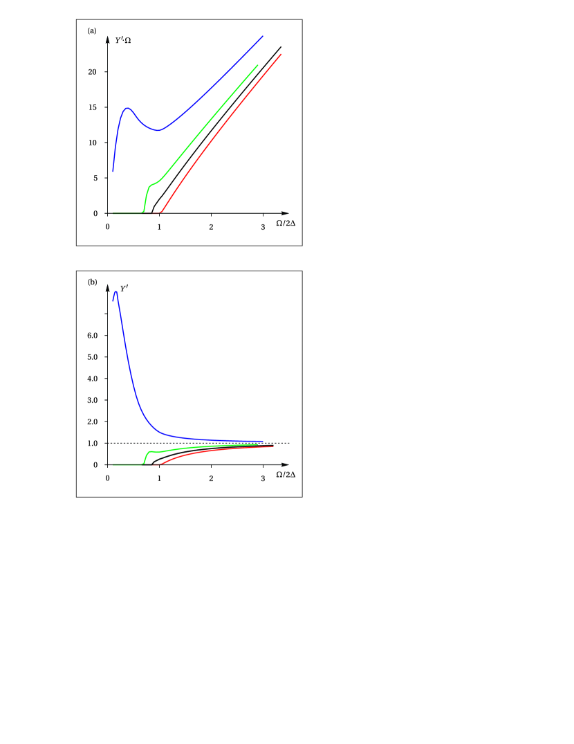
Figure 4: (Color online.) (a) Frequency dependence of the product $Y^{\prime}(\Omega)\cdot\Omega$ which corresponds to the kernel $Q(\Omega)$ in Fig. 8 of Ref. Abrikosov and Gor’kov, 1959. (b) Frequency dependence of the real part of admittance $Y^{\prime}(\Omega)$ at low temperatures for various values of the phase difference $2\varphi_{0}$. One can see that $Y^{\prime}(\Omega)$ increases with increasing $\Omega$ if the frequency $\Omega$ exceeds a threshold value $\Omega_{\text{Th}}$ which depends on $\varphi_{0}$. In the absence of the phase difference (no supercurrent flows through the JJ) we have ${\Omega_{\text{Th}}=2\Delta/\hbar}$. The curves correspond to ${\cos(2\varphi_{0})=1}$ (red), ${\cos(2\varphi_{0})=0.87}$ (black), ${\cos(2\varphi_{0})=1/\sqrt{2}}$ (green), and ${\cos(2\varphi_{0})=0}$ (blue). At low temperatures, the real part of the admittance $Y^{\prime}(\Omega)$ increases monotonously with increasing $\Omega$ if the latter exceeds $2\Delta$ and ${\varphi_{0}\leq\varphi_{\text{c}}}$, where $\varphi_{\text{c}}$ is the phase difference corresponding to critical current. At ${\varphi_{0}>\varphi_{\text{c}}}$, the admittance has a maximum at small $\Omega$.

In Fig. 4 (a) we desplayed the frequency dependence of the product $Y^{\prime}(\Omega)\Omega$ (where $\Omega$ is normalized to $2\Delta$) which is proportional to the kernel $Q(\Omega)$ in Fig. 8 of Ref. Abrikosov and Gor’kov, 1959, where the kernel $Q$ has been calculated for a uniform dirty superconductor.

In Fig. 4 (b), we present the frequency dependence of the real part of admittance $Y^{\prime}(\Omega)$ (normalized to its value in the normal state) at low temperatures for various values of the phase difference $2\varphi_{0}$. One can see that $Y^{\prime}(\Omega)$ increases with increasing $\Omega$ if the frequency $\Omega$ exceeds a threshold value $\Omega_{\text{Th}}$ which depends on $\varphi_{0}$. In the absence of the phase difference (no supercurrent flows through the JJ) we have ${\Omega_{\text{Th}}=2\Delta/\hbar}$. The curves correspond to ${\cos(2\varphi_{0})=1}$ (red), ${\cos(2\varphi_{0})=0.87}$ (black), ${\cos(2\varphi_{0})=1/\sqrt{2}}$ (green), and ${\cos(2\varphi_{0})=0}$ (blue). At low temperatures, the real part of the admittance $Y^{\prime}(\Omega)$ increases monotonously with increasing $\Omega$ if the latter exceeds $2\Delta$ and ${\varphi_{0}\leq\varphi_{\text{c}}}$, where $\varphi_{\text{c}}$ is the phase difference corresponding to critical current. At ${\varphi_{0}>\varphi_{\text{c}}}$, the admittance has a maximum at small $\Omega$.

As we noted in the Introduction, an interesting behavior of the admittance takes place at low $\Omega$ and high temperatures (${T\gg\Delta}$). The main contribution to the real part $Y^{\prime}(\Omega)$ [see Eq. (57)] stems from $j^{\text{an}}$. Integration over large energies $\epsilon$ (${\epsilon\gg\Delta}$) gives the second term $1/R$ at the right hand side of Eq. (3). In this case, ${F^{R}(\epsilon_{+})\simeq-F^{A}(\epsilon_{-})\simeq\Delta/\epsilon}$, ${G^{R}(\epsilon_{+})\simeq-G^{A}(\epsilon_{-})\simeq 1}$, and ${b^{R}\simeq b^{A}\simeq i\Delta\sin\varphi_{0}/\epsilon^{2}}$. The largest contribution occurs due to the first terms in the square brackets in Eq. (61). Integrating these terms,

$$I_{1\Omega}^{\text{an}} =\frac{i\varphi_{\Omega}}{4eR}\int d\,\bar{\epsilon}[\tanh(\epsilon_{+}\beta)-\tanh(\epsilon_{-}\beta)]$$ (63)

$$\simeq\frac{i\Omega\varphi_{\Omega}}{2eR}\int_{0}^{\infty}d\,\bar{\epsilon}\cosh^{-2}(\bar{\epsilon}\beta)=\frac{V_{\Omega}}{R}\,,$$

we obtain the main contribution to the the admittance $1/R$.

The second important contribution to $Y^{\prime}(\Omega)$ stems from the second term in the square brackets at the right hand side of Eq. (61) in the energy interval

$$\tilde{\Delta}=\Delta\cos\varphi_{0}\leq\epsilon\leq\Delta\,.$$ (64)

In this interval, we have ${F^{R}(\epsilon_{+})-F^{A}(\epsilon_{-})\simeq(\Omega/2+i\nu_{\text{in}})\partial_{\epsilon}F^{R}}$, ${\tilde{\zeta}^{R}=-\tilde{\zeta}^{A}}$ and ${\mathrm{arsinh}\big{(}\frac{\Delta\sin\varphi_{0}}{\zeta^{R}}\big{)}+\mathrm{arsinh}\big{(}\frac{\Delta\sin\varphi_{0}}{\zeta^{A}}\big{)}=-i\pi}$. Therefore, setting $\cosh^{-2}(\epsilon\beta)\approx 1$, we obtain at ${T\gg\Delta}$

$$I_{2\Omega}^{\text{an}} =\frac{2eV_{\Omega}}{\hbar}\frac{\pi\Delta^{2}}{2T}\frac{\gamma_{\epsilon}-i\Omega}{\gamma_{\epsilon}^{2}+\Omega^{2}}\frac{\cos^{2}\varphi_{0}}{\sin\varphi_{0}}\int_{\cos\varphi_{0}}^{1}d\,x\frac{1-x^{2}}{x\sqrt{x^{2}-\cos^{2}\varphi_{0}}}$$ (65)

$$=\frac{2eV_{\Omega}}{\hbar}I_{c}\frac{\gamma_{\epsilon}-i\Omega}{\gamma_{\epsilon}^{2}+\Omega^{2}}P(\varphi_{0})\,,$$

where ${\nu_{\text{in}}=\gamma_{\epsilon}/2}$. Thus, the admittance is given by Eq. (3) with the function $P(\varphi_{0})$ equal to

$$P(\varphi_{0})=\cot(\varphi_{0})[2\varphi_{0}-\sin(2\varphi_{0})]\,.$$ (66)

The function $P(\varphi_{0})$ is shown in Fig. 5.

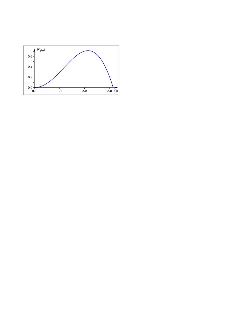
Figure 5: (Color online.) The form of the function of $P(\varphi_{0})$.

The integral in Eq. (63) can be calculated for any temperatures if the factor $\cosh^{-2}(\epsilon\beta)$ in the integrand is taken into account, i.e., not using the approximation ${\cosh^{-2}(\epsilon\beta)\approx 1}$.

Therefore, the deviation $\delta Y^{\prime}(\Omega)$ of the real part of the admittance $Y^{\prime}(\Omega)$ from its value in the normal state $(1/R)$ is

$$\delta Y^{\prime}(\Omega)R=\frac{2eI_{\text{c}}R}{\hbar}\frac{\gamma_{\epsilon}}{\gamma_{\epsilon}^{2}+\Omega^{2}}P(\varphi_{0})\,.$$ (67)

The normalized deviation ${\delta\tilde{Y}^{\prime}(\Omega)\equiv\delta Y^{\prime}(\Omega)R}$ has a maximum at ${\Omega=0}$ with a magnitude ${\delta\tilde{Y}^{\prime}(\Omega)_{\max}\simeq 2eI_{\text{c}}R/\hbar\nu_{\text{in}}\simeq\Delta^{2}/(T\hbar\nu_{\text{in}})}$ which can be much larger than 1. The enhancement of the admittance, Eq. (67), is caused by quasiparticles with energies in the interval defined by Eq. (64).

It is of interest to calculate the density of states (DOS) $N(\epsilon,x)$ in the junction and its spatial dependence. Note that this dependence cannot be found in tunnel Hamiltonian approach. The function $N(\epsilon,x)$ is zero at energies ${|\epsilon|\leq\tilde{\Delta}}$, but is finite at energies ${|\epsilon|\geq\tilde{\Delta}}$. In this energy range, ${\tilde{\Delta}\leq|\epsilon|\leq\Delta}$, the DOS $N_{<}(\epsilon,x)$ is given by (see Appendix C and Ref. Aslamazov and Volkov, 1986)

$$N_{<}(\epsilon,x)=\frac{|\epsilon|}{\sqrt{\epsilon^{2}-\tilde{\Delta}^{2}}}\cosh(\tilde{x}\ln M_{<})\cos\Big{(}\frac{\pi}{2}\tilde{x}\Big{)}\,,$$ (68)

where the function $M_{<}$ is

$$M_{<}=\frac{\Delta\sin\varphi_{0}+\sqrt{\epsilon^{2}-\Delta^{2}\cos^{2}\varphi_{0}}}{\sqrt{\Delta^{2}-\epsilon^{2}}}\,.$$ (69)

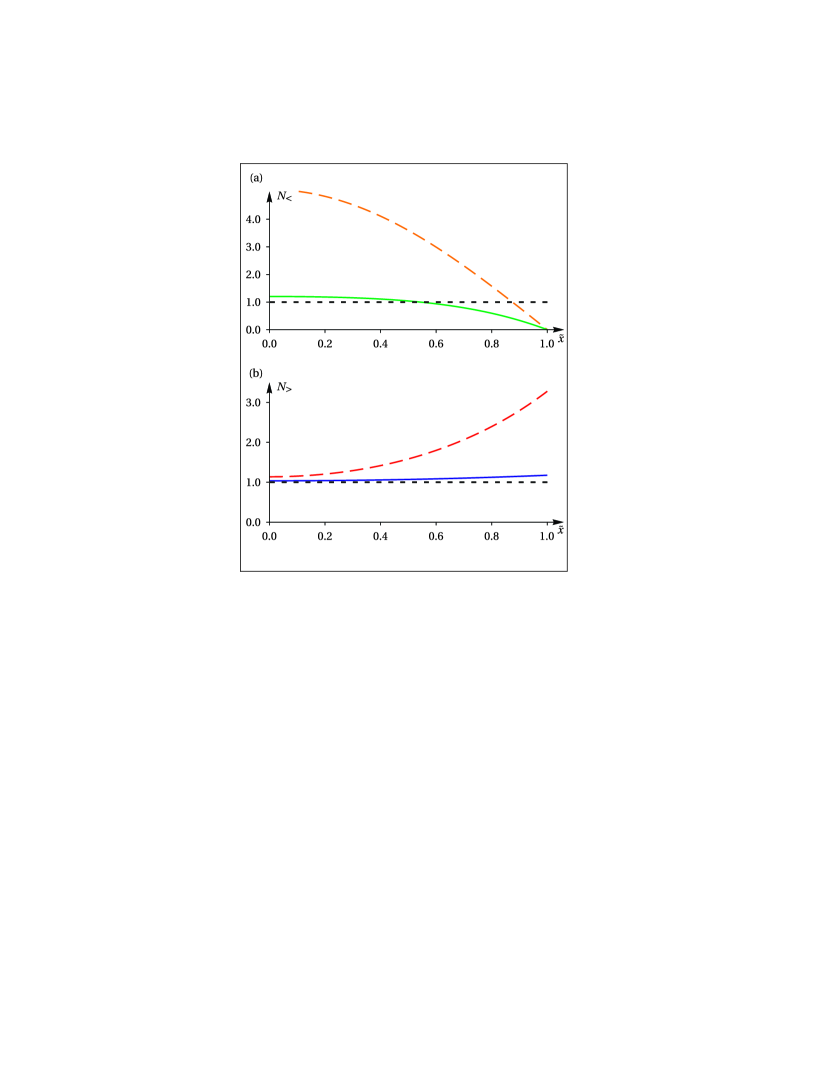
Figure 6: (Color online.) Density of states as a function of the coordinate ${\tilde{x}=x/L}$: (a) for ${\cos(\varphi_{0})<E<1}$ with the curves corresponding to the values ${E=0.51}$ (long-dashed orange) and ${E=0.9}$ (solid green); (b) for ${E>1}$ with the curves corresponding to the values ${E=1.05}$ (long-dashed red) and ${E=1.9}$ (solid blue). The short-dashed black curve denotes in both cases the value ${N=1}$. We set ${\cos\varphi_{0}=0.5}$.

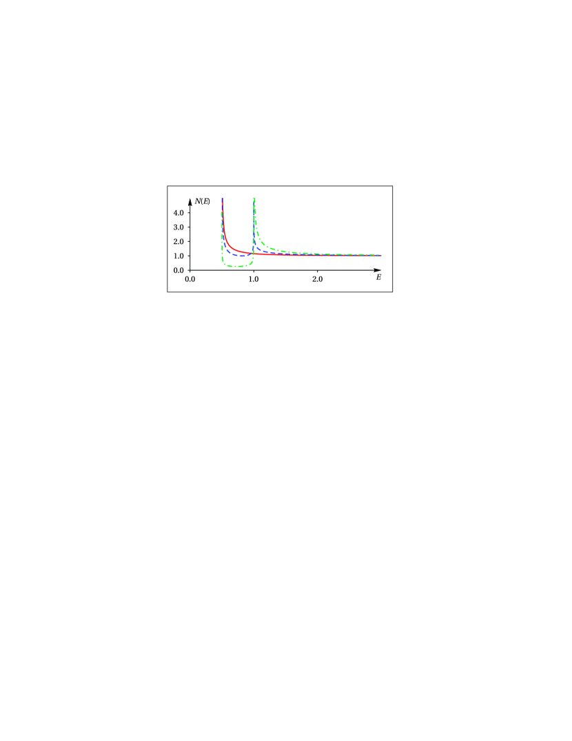
Figure 7: (Color online.) Density of states as a function of the normalized energy ${E=\epsilon/\Delta}$ for different values of the coordinate ${\tilde{x}=x/L}$, i.e., ${\tilde{x}=0}$ (solid red), ${\tilde{x}=0.5}$ (dashed blue), and ${\tilde{x}=0.9}$ (dash-dotted green). We set ${\cos\varphi_{0}=0.5}$.

We plot the DOS $N_{<}(\epsilon,x)$ for different ${E\equiv\epsilon/\Delta}$ in Fig. 6 (a). As it should be, at ${x=\pm L}$, the DOS turns to zero. At energies $\epsilon$ below the gap $\tilde{\Delta}$ (${|\epsilon|\leq\tilde{\Delta}}$) in the center of the junction the DOS is also zero. Above the gap $\Delta$ (${|\epsilon|\geq\Delta}$) the DOS is

$$N_{>}(\epsilon,x)=\frac{|\epsilon|}{\sqrt{\epsilon^{2}-\tilde{\Delta}^{2}}}\cosh(\tilde{x}\ln M_{>})\,,$$ (70)

where

$$M_{>}=\frac{\Delta\sin\varphi_{0}+\sqrt{\epsilon^{2}-\Delta^{2}\cos^{2}\varphi_{0}}}{\sqrt{\epsilon^{2}-\Delta^{2}}}\,.$$ (71)

The DOS $N_{>}(\epsilon,x)$ for different $E$ is shown in Fig. 6 (b).

In Fig. 7 we plot the dependence of the DOS on the energy ${E\equiv\epsilon/\Delta}$ for different values of $\tilde{x}$. In a ballistic case, the function $N(\epsilon)$ has sharp peaks at energies corresponding to the positions of Andreev’s levels. In the considered diffusive case these peaks are smeared out by impurity scattering so that the dependence $N(\epsilon)$ is a smooth curve having singularities at the edges, ${\epsilon=\Delta\cos\varphi_{0}}$ and ${\epsilon=\Delta}$.

V Conclusions

We analyzed the admittance $Y(\Omega)$ of short weak links of two types. The first one is a one-dimensional superconducting wire with a local suppression of the superconducting order parameter $|\Psi|$. This system resembles a phase-slip center or a one-dimensional Larkin-Ovchinnikov-Fulde-Ferrell structure. We calculated $Y$ and the impedance ${Z=Y^{-1}}$ on the basis of non-stationary Ginzburg-Landau equations.Gor’kov and Eliashberg (1968) Ac current through this wire induces a condensate momentum $Q_{\Omega}$ and an inhomogeneity of $|\Psi|$ leads to branch imbalance $n_{\text{imb}}$ and to the appearance of another gauge-invariant quantity, the potential $\mu$, proportional to $n_{\text{imb}}$.

As we mentioned in the Introduction, the branch-imbalance, i.e., the unequal population of the electron- and hole-like branches of the excitation spectrum, arises in nonuniform superconductors when a conversion of the supercurrent $j_{S}$ into the quasiparticle current $j_{N}$ takes place (see Refs. Tinkham and Clarke, 1972; Tinkham, 1972; Schmid and Schön, ; Artemenko and Volkov, 1979). The typical examples of such a conversion are the passage of the charge current through the S/N boundary,Schmid and Schön ; Artemenko et al. (1978); Ovchinnikov (1978) or collective phase mode, i.e., Carlson-Goldman mode,Carlson and Goldman (1975) in uniform superconductors.Schmid and Schön (1975); Artemenko and Volkov (1975, 1979); Sch n (1986) In the latter case, nonuniform perturbations of the the currents $j_{N}$ and $j_{S}$ propagate with a finite wave vector $k$ converting into each other so that the total current density ${j=j_{N}+j_{S}}$ is not perturbed, ${j=0}$.

The electric field $E$, which arises in the wire (see Fig. 1), is caused by both quantities, $Q_{\Omega}$ and $\partial_{x}\mu$ so that neither of these quantities can be neglected (compare with a recent paper, Ref. Dai and Lee, 2017, where only the quantity ${\mathbf{Q}\propto\mathbf{A}}$ was taken into account). The real part of the impedance $Z^{\prime}$ has a maximum at some frequency $\Omega_{m}$ which decreases with increasing suppression of $|\Psi|$.

We also analyzed ac properties of short Josephson S-c-S weak links. The admittance $Y(\Omega)$ is described by an expression that has been obtained on the basis of microscopic equations for quasiclassical Green’s function in the Keldysh technique.Artemenko et al. (1979) The obtained dependence $Y(\Omega)$ is valid in a wide range of the frequencies $\Omega$ and temperatures $T$ provided the Thouless energy ${E_{\text{Th}}=D/L^{2}}$ exceeds $\Delta$, $T$, and $\hbar\Omega$.

At low temperatures $T$, the absorption is absent (${Y^{\prime}=0}$) if the energy of photons $\hbar\Omega$ is less than the lowest energy gap in the center of the constriction ${\tilde{\Delta}=\Delta\cos\varphi_{0}}$. With increasing the difference ${(\hbar\Omega-\tilde{\Delta})}$, the absorption monotonously increases if the phase difference $2\varphi_{0}$ is less than the phase difference $2\varphi_{\text{c}}$ corresponding to a maximum of the Josephson current ${I_{\text{J}}=I_{\text{c}}}$. In the interval ${2\varphi_{\text{c}}<2\varphi_{0}<\pi}$, the dependence of $Y^{\prime}(\Omega)$ has a maximum.

The hump in the obtained dependence $Y^{\prime}(\Omega)$ is much broader than the peak in absorption in a current-carrying superconductor.Moor et al. (2017) The mechanisms causing these maxima are different. In the first case, the maximum stems from excitation of quasiparticles with energy range defined by Eq. (64). These quasiparticles are bound in a potential well within the constriction. In the second case, in Ref. Moor et al., 2017, the peak is related to a resonance excitation of the Higgs mode by an ac field.

The anomalous enhancement of the real part of the admittance $Y^{\prime}(\Omega)$ at low frequencies $\Omega$ described by Eq. (67), is caused by interference of Cooper pairs and quasiparticles with energies in the interval determined by Eq. (64). These quasiparticles experience multiple Andreev reflections. In the ballistic case, the quasiparticles occupy Andreev’s levels.Gunsenheimer and Zaikin (1994); Bratus’ et al. (1995); Cuevas et al. (1996) In the diffusive case, these levels are broadened by impurity scatteringBardas and Averin (1997); Kos et al. (2013) so that the peaks in the DOS $N(\epsilon,x)$ corresponding to Andreev’s levels disappear, and the function $N(\epsilon,x)$ is a smooth function with singularities at ${\epsilon=\Delta\cos\varphi_{0}}$ and ${\epsilon=\Delta}$. In the latter case, anomalous behaviour of low energy quasiparticles results in a singularity of dc conductance at ${V\to 0}$.Bardas and Averin (1997)

The enhancement of $Y^{\prime}(\Omega)$ at low frequencies results in an enhancement of the supercurrent noise because the real part of admittance and spectral function of noise are connected by the fluctuation-dissipation theorem. The anomalous noise in Josephson weak links has been studied in detail in many papers.Averin and Imam (1996); Martín-Rodero et al. (1996); Cuevas et al. (1999); Naveh and Averin (1999); Belzig and Nazarov (2001); Bezuglyi et al. (2003)

Note an important circumstance. In a current-biased S-c-S JJ, the states with phase difference ${2\varphi_{\text{c}}<2\varphi_{0}}$ are unstable, so that it is impossible to observe a non-monotonous dependence of absorption in these junctions. However, in recent experimentsDassonneville et al. (2013); Ronzani et al. (2016) it was shown that the phase difference $2\varphi_{0}$ in the interval

$$2\varphi_{\text{c}}<2\varphi_{0}<\pi$$ (72)

is reachable. Thus, it would be interesting to observe a non-monotonous dependence of absorption in such JJs by appropriate adjustment of the phase difference $2\varphi_{0}$ with the help of an external magnetic field. In these experiments, the S-c-S Josephson weak link was incorporated into a superconducting loop. The phase difference is determined by a magnetic field $H_{0}$ through this loop,

$$2\varphi_{0}=2\pi\Big{(}n+\frac{\Phi}{\Phi_{0}}\Big{)}\,,$$ (73)

where ${\Phi=H_{0}S+\mathcal{L}I_{\text{J}}}$ is the magnetic flux through the loop, and $S$ respectively $\mathcal{L}$ are the area respectively inductance of the loop.

Therefore, the absorption can be studied in the setup used in Ref. Ronzani et al., 2016 if the magnetic field contains not only dc but also an ac component, ${H(t)=H_{0}+H_{\Omega}\cos(\Omega t)}$. Qualitatively, our results are applicable to the system studied in Ref. Ronzani et al., 2016 because the length of the constriction $2L$ (${2L\approx 160\text{nm}}$) is comparable with the coherence length ${\xi_{\text{S}}\approx 100\text{nm}}$. By varying $H_{0}$, one can change the phase $\varphi_{0}$ using the relation in  Eq. (73) and study the absorption of the ac component $H_{\Omega}\cos(\Omega t)$ as a function of the frequency $\Omega$.

At high temperatures (${T\gg\Delta}$), the main contribution to the admittance $Y_{\Omega}$ occurs due to the anomalous term. Quasiparticles with large enough energies (${\epsilon\geq\Delta}$) yield the admittance $Y^{\prime}$ approximately equal to that in the normal state ${Y_{\text{n}}^{\prime}=1/R}$, whereas quasiparticles with energy range defined by Eq. (64) lead to an enhanced admittance $\delta Y^{\prime}$ at low $\Omega$ which can exceed $Y_{\text{n}}^{\prime}$ by $\Delta/\gamma_{\text{in}}$ times. The dependence of $\delta Y^{\prime}$ on dc current (or phase difference) is described by an analytical expression, Eq. (67).

Appendix A Ginzburg-Landau equation

Linearizing Eqs. (14)–(17) we obtain the set of equations for the function $\delta E_{\Omega}$,

$$\nu f_{0}^{2}(x)\mu_{\Omega} =-\partial_{x}\delta E_{\Omega}\,,$$ (74)

$$\delta Q_{\Omega}f_{0}^{2}(x)+Q_{\infty}[f_{0}^{2}(x)-1] =-\delta E_{\Omega}\,,$$ (75)

$$-i\Omega\delta Q_{\Omega} =\delta E_{\Omega}+\partial_{x}\mu_{\Omega}\,.$$ (76)

Excluding $\delta Q_{\Omega}$ and $\mu_{\Omega}$, we get

$$\delta E_{\Omega}\nu\big{[}f_{0}^{2}(x)-i\Omega\big{]}-\Big{[}\partial_{xx}^{2}\delta E_{\Omega}-2\frac{\partial_{x}f_{0}(x)}{f_{0}(x)}\partial_{x}\delta E_{\Omega}\Big{]}=-i\Omega Q_{\infty}\nu\big{[}1-f_{0}^{2}(x)\big{]}\,.$$ (77)

One can exclude the first derivative $\partial_{x}\delta E_{\Omega}$ via the transformation ${\delta E_{\Omega}=f_{0}(x)\mathcal{E}_{\Omega}}$. Thus, an “effective electric field” $\mathcal{E}_{\Omega}$ satisfies the equation

$$-\partial_{xx}^{2}\mathcal{E}_{\Omega}+\mathcal{E}_{\Omega}\Big{[}\nu\big{(}f_{0}^{2}(x)-i\Omega\big{)}+2\Big{(}\frac{\partial_{x}f_{0}(x)}{f_{0}(x)}\Big{)}^{2}-\frac{\partial_{xx}^{2}f_{0}(x)}{f_{0}(x)}\Big{]}=-i\Omega I_{\Omega}\frac{\nu\big{[}1-f_{0}^{2}(x)\big{]}}{f_{0}(x)[1-i\Omega]}\,.$$ (78)

Using the expression Eq. (20) for $f_{0}(x)$, we obtain Eq. (26).

At ${x=0}$, the function $\mathcal{E}_{\Omega}$ is continuous, while $\partial_{x}\mathcal{E}_{\Omega}$ has a jump. It can be found directly from Eq. (19)

$$\big{[}\partial_{x}\mathcal{E}_{\Omega}\big{]} =2\partial_{x}\mathcal{E}_{\Omega}|_{0+}$$ (79)

$$=-\frac{\partial_{x}f_{0}(x)}{f_{0}(0)}\mathcal{E}_{\Omega}(x)|_{x=0}$$

$$=-a_{0}\mathcal{E}_{\Omega}(0)\,,$$

where ${\big{[}\partial_{x}\mathcal{E}_{\Omega}\big{]}\equiv\partial_{x}\big{(}\mathcal{E}_{\Omega}|_{x=0+}-\mathcal{E}_{\Omega}|_{x=0-}\big{)}}$, see also Eq. (27).

Appendix B Expression for the current

In the first step, it is necessary to find the functions $\delta\hat{a}^{R(A)}$. From the normalization condition Eq. (9) we get

$$[\hat{a}\cdot\hat{g}+\hat{g}\cdot\hat{a}]^{R(A)}=0\,.$$ (80)

Linearizing this equation, we obtain for deviations caused by the ac perturbation of the phase $\varphi_{\Omega}$

$$[\delta\hat{a}\cdot\hat{g}+\hat{g}\cdot\delta\hat{a}]^{R(A)}=-[\hat{a}_{0}\cdot\delta\hat{g}+\delta\hat{g}\cdot\hat{a}_{0}]^{R(A)}\,,$$ (81)

where the matrices $\hat{a}_{0}^{R(A)}$ are determined by Eq. (49). We took into account that neither $\hat{a}_{0}$ nor $\delta\hat{a}$ do not depend on the coordinate $x$. Then, we subtract Eq. (81) from itself taken at different points ${x=\pm L}$,

$$\big{[}\delta\hat{a}\cdot\hat{G}_{\varphi}^{(-)}+\hat{G}_{\varphi}^{(-)}\cdot\delta\hat{a}\big{]}^{R(A)}=-\big{[}\hat{a}_{0}\cdot\delta\hat{G}^{(-)}+\delta\hat{G}^{(-)}\cdot\hat{a}_{0}\big{]}^{R(A)}\,.$$ (82)

The matrix $\hat{G}_{\varphi}^{(-)}$ is defined as

$$\hat{G}_{\varphi}^{(-)}=\big{[}\hat{G}_{\varphi}(L)-\hat{G}_{\varphi}(-L)\big{]}^{R(A)}/2$$ (83)

with ${\hat{G}_{\varphi}^{R(A)}(\pm L)=\big{[}G(\epsilon)\hat{\tau}_{3}+F(\epsilon)i(\hat{\tau}_{2}\cos\varphi_{0}\pm\hat{\tau}_{1}\sin\varphi_{0})\big{]}^{R(A)}}$, and, thus, the matrix $\hat{G}{(-)}$ is given by Eq. (53).

The deviation $\delta\hat{G}^{(-)}$ due to a small phase perturbations $\varphi_{\Omega}$ is found from Eq. (47),

$$\delta\hat{G}^{(-)} =\delta\big{[}(1+i\hat{\tau}_{3}\varphi_{\Omega})\hat{G}_{\text{st}}^{(-)}(1-i\hat{\tau}_{3}\varphi_{\Omega})\big{]}$$ (84)

$$=\varphi_{\Omega}i\big{[}-\hat{\tau}_{0}(G_{+}-G_{-})+\hat{\tau}_{1}(F_{+}+F_{-})\cos\varphi_{0}\big{]}\,,$$

where ${G_{\pm}\equiv G_{0}(\epsilon_{\pm})}$, ${\epsilon_{\pm}=\bar{\epsilon}\pm\Omega/2}$. As follows from Eq. (41), we need to find $\mathrm{Tr}\{\hat{\tau}_{3}\hat{a}\}$. Thus, multiplying Eq. (56) by $i\hat{\tau}_{2}$ and calculating the trace, we find

$$\frac{1}{2}\mathrm{Tr}\{\hat{\tau}_{3}\hat{a}\}^{R(A)}=\frac{l\varphi_{\Omega}\big{\{}(b_{+}\epsilon_{+}+b_{-}\epsilon_{-})(G_{+}-G_{-})-\Delta\cos^{2}\varphi_{0}(F_{+}+F_{-})(b_{+}-b_{-})\big{\}}^{R(A)}}{L(F_{+}-F_{-})^{R(A)}\sin\varphi_{0}}\,.$$ (85)

The same equation holds for $\mathrm{Tr}\{\hat{\tau}_{3}\hat{a}^{\text{an}}\}$ if all functions like $G_{-}^{R}$ in Eq. (83) for $\hat{a}^{R}$ are replaced by $G_{-}^{A}$.

Appendix C Density of states in an S-c-S type contact

The density of states is determined by the expression

$$N(\epsilon)=\frac{1}{4}\mathrm{Tr}\big{\{}\hat{\tau}_{3}(\hat{g}^{R}(\epsilon,x)-\hat{g}^{A}(\epsilon,x))\big{\}}\,,$$ (86)

where $\hat{g}^{R(A)}(\epsilon,x)$ are determined by Eq. (42) which can be written in the form (dropping the indices $R(A)$)

$$\hat{g}(\epsilon,x)=\hat{g}(\epsilon,0)\big{[}\cosh[l^{-1}x\hat{a}(\epsilon)]-\sinh[l^{-1}x\hat{a}(\epsilon)]\big{]}\,,$$ (87)

where the functions $\cosh[l^{-1}x\hat{a}(\epsilon)]$ and $\sinh[l^{-1}x\hat{a}(\epsilon)]$ can be presented as follows

$$\cosh[l^{-1}x\hat{a}(\epsilon)] =\cosh\Big{(}\frac{x}{L}A\Big{)}\,,$$ (88)

$$\sinh[l^{-1}x\hat{a}(\epsilon)] =\frac{\hat{m}}{i\tilde{\zeta}(\epsilon)}\sinh\Big{(}\frac{x}{L}A\Big{)}\,,$$ (89)

where we defined ${A=\mathrm{arsinh}\big{[}\zeta^{-1}(\epsilon)\Delta\sin\varphi_{0}\big{]}=\ln M}$ with ${M=\zeta^{-1}(\epsilon)\big{[}\Delta\sin\varphi_{0}+\tilde{\zeta}(\epsilon)\big{]}}$, and ${\hat{m}=\tilde{\Delta}\hat{\tau}_{3}+\epsilon i\hat{\tau}_{2}}$. We used the expression for the matrix $\hat{a}$ from Ref. Artemenko et al., 1979,

$$\hat{a}=-\frac{il}{L\tilde{\zeta}(\epsilon)}\hat{m}A\,.$$ (90)

The matrix $\hat{g}(\epsilon,0)$ is found from Eq. (44),

$$\hat{g}(\epsilon,0)=\frac{\hat{G}^{(+)}}{\cosh A}\,.$$ (91)

Therefore, Eq. (87) can be written in the form

$$\hat{g}(\epsilon,x)=\frac{\hat{G}_{+}}{\cosh A}\Big{[}\cosh(\tilde{x}A)+\frac{\hat{m}}{i\tilde{\zeta}(\epsilon)}\sinh(\tilde{x}A)\Big{]}\,.$$ (92)

Using Eq. (86) we obtain for the density of states

$$N(\epsilon,x)=\frac{1}{2}\Bigg{\{}\Big{[}g(\epsilon)\frac{\cosh(\tilde{x}\ln M)}{\cosh(\ln M)}\Big{]}^{R}-\Big{[}g(\epsilon)\frac{\cosh(\tilde{x}\ln M)}{\cosh(\ln M)}\Big{]}^{A}\Bigg{\}}\,.$$ (93)

One can easily show that ${\cosh(\ln M)=\tilde{\zeta}(\epsilon)\zeta^{-1}(\epsilon)}$. Therefore, the density of states $N(\epsilon,x)$ for ${|\epsilon|\geq\Delta}$ when ${\tilde{\zeta}^{R}(\epsilon)=-\tilde{\zeta}^{A}(\epsilon)}$ can be written as follows

$$N(\epsilon,x)=\frac{|\epsilon|}{2\tilde{\zeta}(\epsilon)}\big{\{}\big{[}\cosh(\tilde{x}\ln M)\big{]}^{R}+\big{[}\cosh(\tilde{x}\ln M)\big{]}^{A}\big{\}}\,.$$ (94)

Consider two cases:

1. ${|\epsilon|\geq\Delta}$. In this case, ${M^{R}=\big{[}M^{A}\big{]}^{-1}\equiv M_{>}}$, where ${M_{>}=\zeta_{>}^{-1}(\epsilon)\big{[}\Delta\sin\varphi_{0}+\tilde{\zeta}_{>}(\epsilon)\big{]}}$ with ${\tilde{\zeta}_{>}(\epsilon)=\sqrt{\epsilon^{2}-\tilde{\Delta}^{2}}}$, and ${\zeta_{>}(\epsilon)=\sqrt{\epsilon^{2}-\Delta^{2}}}$. We obtain

   $$N(\epsilon,x) =\frac{|\epsilon|}{\tilde{\zeta}(\epsilon)}\cosh\big{(}\tilde{x}\ln M_{>}\big{)}$$ (95)

   $$=\frac{|\epsilon|}{2\tilde{\zeta}(\epsilon)}\big{[}M_{>}^{\tilde{x}}+M_{>}^{-\tilde{x}}\big{]}\,.$$

2. ${\tilde{\Delta}\leq|\epsilon|\leq\Delta}$. In this case, ${M^{R}=-i\zeta_{<}^{-1}(\epsilon)\big{[}\Delta\sin\varphi_{0}+\tilde{\zeta}_{>}(\epsilon)\big{]}\equiv-iM_{<}}$ and ${M^{A}=-i\zeta_{<}^{-1}(\epsilon)[\Delta\sin\varphi_{0}-\tilde{\zeta}_{>}(\epsilon)]}$, and one can write the sum in Eq. (94) in the form

   $$\big{[}\cosh(\tilde{x}\ln M)\big{]}^{R}+\big{[}\cosh(\tilde{x}\ln M)\big{]}^{A} =2\cosh\Big{[}\frac{\tilde{x}}{2}\big{(}M^{R}+M^{A}\big{)}\Big{]}\cosh\Big{[}\frac{\tilde{x}}{2}\big{(}M^{R}-M^{A}\big{)}\Big{]}$$ (96)

   $$=2\cos\Big{(}\frac{\pi\tilde{x}}{2}\Big{)}\cosh\big{[}\tilde{x}\ln M_{<}\big{]}\,.$$ (97)

Combining Eqs. (94)–(96) we obtain Eq. (68).

References

- Bardeen et al. (1957) J. Bardeen, L. N. Cooper, and J. R. Schrieffer, Phys. Rev. 108, 1175 (1957).
- Mattis and Bardeen (1958) D. C. Mattis and J. Bardeen, Phys. Rev. 111, 412 (1958).
- Abrikosov et al. (1958) A. A. Abrikosov, L. P. Gor’kov, and I. M. Khalatnikov, Sov. Phys. JETP 8, 182 (1958).
- Abrikosov and Gor’kov (1959) A. A. Abrikosov and L. P. Gor’kov, Sov. Phys. JETP 8, 1090 (1959).
- Nam (1967a) S. B. Nam, Phys. Rev. 156, 470 (1967a).
- Nam (1967b) S. B. Nam, Phys. Rev. 156, 487 (1967b).
- Higgs (1964) P. W. Higgs, Phys. Rev. Lett. 13, 508 (1964).
- Volkov and Kogan (1974) A. F. Volkov and S. M. Kogan, Sov. Phys. JETP 38, 1018 (1974).
- Kulik et al. (1981) I. O. Kulik, O. Entin-Wohlman, and R. Orbach, Journal of Low Temperature Physics 43, 591 (1981).
- Barankov et al. (2004) R. A. Barankov, L. S. Levitov, and B. Z. Spivak, Phys. Rev. Lett. 93, 160401 (2004).
- Barankov and Levitov (2006) R. A. Barankov and L. S. Levitov, Phys. Rev. Lett. 96, 230403 (2006).
- Amin et al. (2004) M. H. S. Amin, E. V. Bezuglyi, A. S. Kijko, and A. N. Omelyanchouk, Low Temperature Physics 30, 661 (2004).
- Warner and Leggett (2005) G. L. Warner and A. J. Leggett, Phys. Rev. B 71, 134514 (2005).
- Szymańska et al. (2005) M. H. Szymańska, B. D. Simons, and K. Burnett, Phys. Rev. Lett. 94, 170402 (2005).
- Yuzbashyan et al. (2005) E. A. Yuzbashyan, B. L. Altshuler, V. B. Kuznetsov, and V. Z. Enolskii, Phys. Rev. B 72, 220503 (2005).
- Yuzbashyan et al. (2006) E. A. Yuzbashyan, O. Tsyplyatyev, and B. L. Altshuler, Phys. Rev. Lett. 96, 097005 (2006).
- Yuzbashyan and Dzero (2006) E. A. Yuzbashyan and M. Dzero, Phys. Rev. Lett. 96, 230404 (2006).
- Yuzbashyan (2008) E. A. Yuzbashyan, Phys. Rev. B 78, 184507 (2008).
- Gurarie (2009) V. Gurarie, Phys. Rev. Lett. 103, 075301 (2009).
- Krull et al. (2014) H. Krull, D. Manske, G. S. Uhrig, and A. P. Schnyder, Phys. Rev. B 90, 014515 (2014).
- Moor et al. (2014) A. Moor, P. A. Volkov, A. F. Volkov, and K. B. Efetov, Phys. Rev. B 90, 024511 (2014).
- Dzero et al. (2015) M. Dzero, M. Khodas, and A. Levchenko, Phys. Rev. B 91, 214505 (2015).
- Yuzbashyan et al. (2015) E. A. Yuzbashyan, M. Dzero, V. Gurarie, and M. S. Foster, Phys. Rev. A 91, 033628 (2015).
- Peronaci et al. (2015) F. Peronaci, M. Schiró, and M. Capone, Phys. Rev. Lett. 115, 257001 (2015).
- Kemper et al. (2015) A. F. Kemper, M. A. Sentef, B. Moritz, J. K. Freericks, and T. P. Devereaux, Phys. Rev. B 92, 224517 (2015).
- Tsuji and Aoki (2015) N. Tsuji and H. Aoki, Phys. Rev. B 92, 064508 (2015).
- Cea et al. (2015) T. Cea, C. Castellani, G. Seibold, and L. Benfatto, Phys. Rev. Lett. 115, 157002 (2015).
- Cea et al. (2016) T. Cea, C. Castellani, and L. Benfatto, Phys. Rev. B 93, 180507 (2016).
- Murakami et al. (2016) Y. Murakami, P. Werner, N. Tsuji, and H. Aoki, Phys. Rev. B 93, 094509 (2016).
- Sentef et al. (2016) M. A. Sentef, A. F. Kemper, A. Georges, and C. Kollath, Phys. Rev. B 93, 144506 (2016).
- Chou et al. (2016) Y.-Z. Chou, Y. Liao, and M. S. Foster, ArXiv e-prints (2016), arXiv:1611.07089 [cond-mat.supr-con] .
- Yoon and Watanabe (2015) S. Yoon and G. Watanabe, ArXiv e-prints (2015), arXiv:1512.09058 [cond-mat.quant-gas] .
- Matsunaga et al. (2013) R. Matsunaga, Y. I. Hamada, K. Makise, Y. Uzawa, H. Terai, Z. Wang, and R. Shimano, Phys. Rev. Lett. 111, 057002 (2013).
- Matsunaga et al. (2014) R. Matsunaga, N. Tsuji, H. Fujita, A. Sugioka, K. Makise, Y. Uzawa, H. Terai, Z. Wang, H. Aoki, and R. Shimano, Science 345, 1145 (2014).
- Moor et al. (2017) A. Moor, A. F. Volkov, and K. B. Efetov, Phys. Rev. Lett. 118, 047001 (2017).
- Dai and Lee (2017) Z. Dai and P. A. Lee, Phys. Rev. B 95, 014506 (2017).
- Fulde and Ferrell (1964) P. Fulde and R. A. Ferrell, Phys. Rev. 135, A550 (1964).
- Larkin and Ovchinnikov (1965) A. I. Larkin and Y. N. Ovchinnikov, Sov. Phys. JETP 20, 762 (1965).
- Gol’tsman et al. (2001) G. N. Gol’tsman, O. Okunev, G. Chulkova, A. Lipatov, A. Semenov, K. Smirnov, B. Voronov, A. Dzardanov, C. Williams, and R. Sobolewski, Applied Physics Letters 79, 705 (2001).
- Day et al. (2003) P. K. Day, H. G. LeDuc, B. A. Mazin, A. Vayonakis, and J. Zmuidzinas, Nature 425, 817 (2003).
- Janssen et al. (2013) R. M. J. Janssen, J. J. A. Baselmans, A. Endo, L. Ferrari, S. J. C. Yates, A. M. Baryshev, and T. M. Klapwijk, Applied Physics Letters 103, 203503 (2013).
- Clarke and Wilhelm (2008) J. Clarke and F. K. Wilhelm, Nature 453, 1031 (2008).
- Likharev (1979) K. K. Likharev, Rev. Mod. Phys. 51, 101 (1979).
- Barone and Patern (1982) A. Barone and G. Patern , “Weak superconductivity — phenomenological aspects,” in Physics and Applications of the Josephson Effect (Wiley-VCH Verlag GmbH & Co. KGaA, New York, 1982) pp. 1–24.
- Artemenko et al. (1979) S. N. Artemenko, A. F. Volkov, and A. V. Zaitsev, Sov. Phys. JETP 49, 924 (1979).
- Kulik and Omel’yanchuk (1978) I. O. Kulik and A. N. Omel’yanchuk, Sov. Journal of Low Temperature Physics 4, 142 (1978).
- Kos et al. (2013) F. Kos, S. E. Nigg, and L. I. Glazman, Phys. Rev. B 87, 174521 (2013).
- Dorokhov (1984) O. Dorokhov, Solid State Communications 51, 381 (1984).
- Lempitskii (1983) S. Lempitskii, Sov. Phys. JETP 58, 624 (1983).
- Nagaev (1988) K. E. Nagaev, Fizika Nizkikh Temperatur 14, 1153 (1988).
- Virtanen et al. (2011) P. Virtanen, F. S. Bergeret, J. C. Cuevas, and T. T. Heikkilä, Phys. Rev. B 83, 144514 (2011).
- Tikhonov and Feigel’man (2015) K. S. Tikhonov and M. V. Feigel’man, Phys. Rev. B 91, 054519 (2015).
- Ivlev and Kopnin (1984) B. I. Ivlev and N. B. Kopnin, Advances in Physics 33, 47 (1984).
- Arutyunov et al. (2008) K. Arutyunov, D. Golubev, and A. Zaikin, Physics Reports 464, 1 (2008).
- Tinkham and Clarke (1972) M. Tinkham and J. Clarke, Phys. Rev. Lett. 28, 1366 (1972).
- Tinkham (1972) M. Tinkham, Phys. Rev. B 6, 1747 (1972).
- (57) A. Schmid and G. Schön, Journal of Low Temperature Physics 20, 207.
- Artemenko and Volkov (1979) S. N. Artemenko and A. F. Volkov, Soviet Physics Uspekhi 22, 295 (1979).
- G. and Gurevich (1974) A. A. G. and V. L. Gurevich, Sov. Phys. Solid State 16, 1722 (1974).
- Gor’kov and Eliashberg (1968) L. P. Gor’kov and G. M. Eliashberg, Sov. Phys. JETP 27, 328 (1968).
- Dassonneville et al. (2013) B. Dassonneville, M. Ferrier, S. Guéron, and H. Bouchiat, Phys. Rev. Lett. 110, 217001 (2013).
- Ronzani et al. (2016) A. Ronzani, C. Altimiras, S. D’Ambrosio, P. Virtanen, and F. Giazotto, ArXiv e-prints (2016), arXiv:1611.06263 [cond-mat.supr-con] .
- Martin and Tinkham (1968) W. S. Martin and M. Tinkham, Phys. Rev. 167, 421 (1968).
- Budzinski et al. (1973) W. V. Budzinski, M. P. Garfunkel, and R. W. Markley, Phys. Rev. B 7, 1001 (1973).
- Ovchinnikov and Isaakyan (1978) Y. N. Ovchinnikov and A. R. Isaakyan, Sov. Phys. JETP 47, 91 (1978).
- Usadel (1970) K. D. Usadel, Phys. Rev. Lett. 25, 507 (1970).
- Kopnin (2001) N. B. Kopnin, Theory of Nonequilibrium Superconductivity, The International Series of Monographs on Physics (Clarendon Press, Oxford, UK, 2001).
- Larkin and Ovchinnikov (1986) A. I. Larkin and Y. N. Ovchinnikov, “Nonequilibrium superconductivity,” (Elsevier, Amsterdam, 1986).
- Rammer and Smith (1986) J. Rammer and H. Smith, Rev. Mod. Phys. 58, 323 (1986).
- Belzig et al. (1999) W. Belzig, F. K. Wilhelm, C. Bruder, G. Sch n, and A. D. Zaikin, Superlattices and Microstructures 25, 1251 (1999).
- Volkov (1971) A. F. Volkov, Sov. Phys. JETP 33, 811 (1971).
- Volkov (1974) A. F. Volkov, Sov. Phys. JETP 66, 758 (1974).
- Aslamazov and Volkov (1986) L. G. Aslamazov and A. F. Volkov, “Nonequilibrium superconductivity,” (Elsevier, Amsterdam, 1986).
- Artemenko et al. (1978) S. N. Artemenko, A. F. Volkov, and A. V. Zaitsev, Journal of Low Temperature Physics 30, 487 (1978).
- Ovchinnikov (1978) Y. N. Ovchinnikov, Journal of Low Temperature Physics 31, 785 (1978).
- Carlson and Goldman (1975) R. V. Carlson and A. M. Goldman, Phys. Rev. Lett. 34, 11 (1975).
- Schmid and Schön (1975) A. Schmid and G. Schön, Phys. Rev. Lett. 34, 941 (1975).
- Artemenko and Volkov (1975) S. N. Artemenko and A. F. Volkov, Sov. Phys. JETP 42, 1130 (1975).
- Sch n (1986) G. Sch n, in Nonequilibrium Superconductivity, Modern Problems in Condensed Matter Sciences, Vol. 12, edited by D. N. Langenberg and A. I. Larkin (Elsevier, Amsterdam, 1986) pp. 589–640.
- Gunsenheimer and Zaikin (1994) U. Gunsenheimer and A. D. Zaikin, Phys. Rev. B 50, 6317 (1994).
- Bratus’ et al. (1995) E. N. Bratus’, V. S. Shumeiko, and G. Wendin, Phys. Rev. Lett. 74, 2110 (1995).
- Cuevas et al. (1996) J. C. Cuevas, A. Martín-Rodero, and A. L. Yeyati, Phys. Rev. B 54, 7366 (1996).
- Bardas and Averin (1997) A. Bardas and D. V. Averin, Phys. Rev. B 56, R8518 (1997).
- Averin and Imam (1996) D. Averin and H. T. Imam, Phys. Rev. Lett. 76, 3814 (1996).
- Martín-Rodero et al. (1996) A. Martín-Rodero, A. L. Yeyati, and F. J. García-Vidal, Phys. Rev. B 53, R8891 (1996).
- Cuevas et al. (1999) J. C. Cuevas, A. Martín-Rodero, and A. L. Yeyati, Phys. Rev. Lett. 82, 4086 (1999).
- Naveh and Averin (1999) Y. Naveh and D. V. Averin, Phys. Rev. Lett. 82, 4090 (1999).
- Belzig and Nazarov (2001) W. Belzig and Y. V. Nazarov, Phys. Rev. Lett. 87, 197006 (2001).
- Bezuglyi et al. (2003) E. V. Bezuglyi, E. N. Bratus’, V. S. Shumeiko, and G. Wendin, “Quantum noise in mesoscopic physics,” in Quantum Noise in Mesoscopic Physics, Nato Science Series II: (Springer Netherlands, 2003) pp. 93–118.