Ignore or Comply? On Breaking Symmetry in Consensus

Abstract

We study consensus processes on the complete graph of $n$ nodes. Initially, each node supports one from opinion from a set of up to $n$ different opinions. Nodes randomly and in parallel sample the opinions of constant many nodes. Based on these samples, they use an update rule to change their own opinion. The goal is to reach consensus, a configuration where all nodes support the same opinion.

We compare two well-known update rules: 2-Choices and $3$-Majority. In the former, each node samples two nodes and adopts their opinion if they agree. In the latter, each node samples three nodes: If an opinion is supported by at least two samples the node adopts it, otherwise it randomly adopts one of the sampled opinions. Known results for these update rules focus on initial configurations with a limited number of colors (say $n^{\frac{1}{3}}$), or typically assume a bias, where one opinion has a much larger support than any other. For such biased configurations, the time to reach consensus is roughly the same for 2-Choices and $3$-Majority.

Interestingly, we prove that this is no longer true for configurations with a large number of initial colors. In particular, we show that $3$-Majority reaches consensus with high probability in $\mathrm{O}\bigl{(}n^{3/4}\cdot\log^{7/8}n\bigr{)}$ rounds, while 2-Choices can need $\Omega\mathopen{}\mathclose{{}\left(n/\log n}\right)$ rounds. We thus get the first unconditional sublinear bound for $3$-Majority and the first result separating the consensus time of these processes. Along the way, we develop a framework that allows a fine-grained comparison between consensus processes from a specific class. We believe that this framework might help to classify the performance of more consensus processes.

Keywords: Distributed Consensus; Randomized Protocols; Majorization Theory; Leader Election

1 Introduction

We study consensus (also known as agreement) processes resulting from executing a simple algorithm in a distributed system. The system consists of $n$ anonymous nodes connected by a complete graph. Initially, each node supports one opinion from the set $[k]\coloneqq\set{1,\dots,k}$. We refer to these opinions as colors. The system state is modeled as a configuration vector $c\in\mathbb{N}_{0}^{k}$, whose $i$-th component $c_{i}$ denotes the number (support) of nodes with color $i$. A consensus process is specified by an update rule that is executed by each node. The goal is to reach a configuration in which all nodes support the same color; the special case where nodes have pairwise distinct colors is leader election, an important primitive in distributed computing. We assume a severely restricted synchronous communication mechanism known as Uniform Pull [DGH⁺87, KSSV00, KDG03]. Here, in each discrete round, nodes independently pull information from some (typically constant) number of randomly sampled nodes. Both the message sizes and the nodes’ local memory must be of size $\mathrm{O}\mathopen{}\mathclose{{}\left(\log k}\right)$.

The so-called Voter process (also known as Polling), uses the most naïve update rule: In every round, each node samples one neighbor independently and uniformly at random and adopts that node’s color. Two further natural and prominent consensus processes are the 2-Choices and the $3$-Majority process. Their corresponding update rules, as executed synchronously by each node, are as follows:

• 2-Choices: Sample two nodes independently and uniformly at random. If the samples have the same color, adopt it. Otherwise, ignore them and keep your current color.

• $3$-Majority: Sample three nodes independently and uniformly at random. If a color is supported by at least two samples, adopt it. Otherwise, adopt the color of one of them at random.

One reason for the interest in these processes is that they represent simple and efficient self-stabilizing solutions for Byzantine agreement [PSL80, Rab83]: achieving consensus in the presence of an adversary that can disrupt a bounded set of nodes each round [BCN⁺14, BCN⁺16, CER14, EFK⁺16]. Further interest stems from the fact that they capture aspects of how agreement is reached in social networks and biological systems [BSDDS10, CER14, FPM⁺02].

At first glance, the above processes look quite different. But a slight reformulation of $3$-Majority’s update rule reveals an interesting connection:

• $3$-Majority (alt.): Sample two nodes independently and uniformly at random. If the samples have the same color, adopt it. Otherwise, sample a new neighbor and adopt its color.

This highlights the fact that $3$-Majority is a combination of 2-Choices and Voter: Each node $u$ performs the update rule of 2-Choices. If the sampled colors do not match, instead of keeping its color, $u$ executes the update rule of Voter. Interestingly enough, both $3$-Majority and 2-Choices behave identical in expectation. In comparison to Voter, both 2-Choices and $3$-Majority exhibit a drift: they favor colors with a large support, for which it is more likely that the first two samples match. In particular, if there is a certain initial bias towards one color, Voter still needs linear time (in $n$) to reach consensus, while both 2-Choices and $3$-Majority can exploit the bias to achieve sublinear time. On the other hand, it is unknown how 2-Choices and $3$-Majority behave when they start from configurations having a large number of colors and no (or small) bias (see Section 1.1 for details).

In this paper, we compare the time 2-Choices and $3$-Majority require to reach consensus. In particular, we prove that there is a polynomial gap between their performance if the bias is small and the number of colors is large (say $\Omega\mathopen{}\mathclose{{}\left(n^{1/3}}\right)$). This result follows from our unconditional sublinear bound for $3$-Majority and an almost linear lower bound for 2-Choices. Details of our results and contribution are given in Section 1.2.

1.1 Related Work

Consensus processes are a quite general model that can be used to study and understand different flavors of “spreading phenomena”, for example the spread of infectious diseases, rumors and opinions in societies, or viruses/worms in computer networks. Apart from the above mentioned processes, such spreading processes include the Moran process [LHN05, DGRS14], contact processes, and classic epidemic processes [BG90, Lig99, Mor16]. This overview concentrates on results concerned with the time needed by Voter, 2-Choices, and $3$-Majority to reach consensus. We also provide a short comparison of these processes and briefly discuss some of the slightly more distant relatives at the end of this section.

Voter

Previous work provides strong results for the time to consensus of the Voter process, even for arbitrary graphs. These results exploit an interesting duality: the time reversal of the Voter process turns out to be the coalescing random walk process (see [HP01, AF02]). The expected runtime of Voter on the complete graph and with nodes of pairwise distinct colors is $\Theta\mathopen{}\mathclose{{}\left(n}\right)$. This follows easily from results for more general graphs and the above mentioned duality: The authors of [CEOR13] provide the upper bound $\mathrm{O}\mathopen{}\mathclose{{}\left(\mu^{-1}\cdot(\log^{4}n+\rho)}\right)$ on the expected coalescing time. Here $\mu$ is the graph’s spectral gap and $\rho=(d_{\operatorname{avg}}\cdot n)^{2}/\sum_{u\in V}d^{2}(u)$, where $d_{\operatorname{avg}}$ denotes the average degree. In [BGKMT16] the authors show that the expected time to consensus is bounded by $\mathrm{O}\mathopen{}\mathclose{{}\left(m/(d_{\min}\cdot\phi)}\right)$. Here, $m$ is the number of edges, $\phi$ the conductance, and $d_{\min}$ the minimal degree.

2-Choices

To the best of our knowledge, the only work that considers the case $k>2$ for 2-Choices is [EFK⁺16]. The authors study the complete graph and show that 2-Choices reaches consensus with high probability in $\mathrm{O}\mathopen{}\mathclose{{}\left(k\cdot\log n}\right)$ rounds, provided that $k=\mathrm{O}\mathopen{}\mathclose{{}\left(n^{\varepsilon}}\right)$ for a small constant $\varepsilon>0$ and an initial bias of $\Omega\mathopen{}\mathclose{{}\left(\sqrt{n\cdot\log n}}\right)$. In [CER14, CER⁺15], the authors consider 2-Choices for $k=2$ on different graphs. For random $d$-regular graphs, [CER14] proves that all nodes agree on the first color in $\mathrm{O}\mathopen{}\mathclose{{}\left(\log n}\right)$ rounds, provided that the bias is $\Omega\bigl{(}n\cdot\sqrt{1/d+d/n}\bigr{)}$. The same holds for arbitrary $d$-regular graphs if the bias is $\Omega\mathopen{}\mathclose{{}\left(\lambda_{2}\cdot n}\right)$, where $\lambda_{2}$ is the second largest eigenvalue of the transition matrix. In [CER⁺15], these results are extended to general expander graphs.

$3$-Majority

All theoretical results for $3$-Majority consider the complete graph. The authors of [BCN⁺14] assume that the bias is $\Omega\bigl{(}\min\set{\sqrt{2k},{(n/\log n)}^{1/6}}\cdot\sqrt{n\log n}\bigr{)}$. Under this assumption, they prove that consensus is reached with high probability in $\mathrm{O}\bigl{(}\min\set{k,{(n/\log n)}^{1/3}}\cdot\log n\bigr{)}$ rounds, and that this is tight if $k\leq{(n/\log n)}^{1/4}$. The only result without bias [BCN⁺16] restricts the number of initial colors to $k=\mathrm{o}\bigl{(}n^{1/3}\bigr{)}$. Under this assumption, they prove that $3$-Majority reaches consensus with high probability in $\mathrm{O}\bigl{(}(k^{2}{(\log n)}^{1/2}+k\log n)\cdot(k+\log n)\bigr{)}$ rounds. Their analysis considers phases of length $\mathrm{O}\bigl{(}k^{2}\log n\bigr{)}$ and shows that, at the end of each phase, one of the initial colors disappears with high probability. Note that this approach – so far the only one not assuming any bias – cannot yield sublinear bounds with respect to $k$.

Comparing the above processes on the complete graph for $k>2$, we see that there are situations where Voter is much slower than 2-Choices or $3$-Majority. Even with a linear bias, Voter is known to have linear runtime. In contrast, whenever there is a sufficient bias towards one color, both 2-Choices and $3$-Majority can exploit this to achieve sublinear runtime. However, to the best of our knowledge there are no unconditional results on 2-Choices and $3$-Majority. All but one results need a minimum bias (at least $\Omega\mathopen{}\mathclose{{}\left(\sqrt{n\log n}}\right)$), and the only approach that works without any bias restricts the number of colors to $k=\mathrm{o}\mathopen{}\mathclose{{}\left(n^{1/3}}\right)$ [BCN⁺16].

A related consensus process is $2$-Median [DGM⁺11]. Here, every node updates its color (a numerical value) to the median of its own value and two randomly sampled nodes. Without assuming any initial bias, the authors show that this process reaches consensus with high probability in $\mathrm{O}\mathopen{}\mathclose{{}\left(\log k\cdot\log\log n+\log n}\right)$ rounds. This is seemingly stronger than the bounds achieved for $3$-Majority and 2-Choices without bias. However, it comes at the price of a complete order on the colors (our processes require colors only to be testable for identity). Moreover, $2$-Median is not self-stabilizing for Byzantine agreement (unlike $3$-Majority and 2-Choices [BCN⁺16, EFK⁺16]): it cannot guarantee validity [BCN⁺16]. Another consensus process is the UndecidedDynamics. Here, each node randomly samples one neighbor and, if the sample has a different color, adopts a special “undecided” color. In subsequent rounds, it tries to find a new (real) color by sampling one random neighbor. The most recent results [BCN⁺15] show that, for a large enough bias, consensus is reached with high probability in at most $\mathrm{O}\mathopen{}\mathclose{{}\left(k\log n}\right)$ rounds. Slightly more involved variants yield improved bounds of $\mathrm{O}\mathopen{}\mathclose{{}\left(\log k\cdot\log n}\right)$ [BFGK16, GP16, EFK⁺16]. However, observe that for $k={n}$ all nodes become undecided with constant probability instead of agreeing on a color.

1.2 Contribution & Approach

In this work, we provide an upper bound on $3$-Majority and a lower bound on 2-Choices that solve two open issues: We give the first unconditional sublinear bound on any of these processes (an open issue from, e.g., [BCN⁺16]) and prove that there can be a polynomial gap between the performance of $3$-Majority and 2-Choices (see Theorem 1 below). One should note that this gap is in stark contrast not only to the expected behavior of both processes (which is identical) but also to the setting when there is a bias towards one color (where both processes exhibit the same asymptotic runtime $\mathrm{O}\mathopen{}\mathclose{{}\left(k\cdot\log n}\right)$; see Section 1.1).

The following theorem states slightly simplified versions of our upper and lower bounds (see Theorem 4 and Theorem 5 for the detailed statements).

Theorem 1 (Simplified).

Starting from an arbitrary configuration, $3$-Majority reaches consensus with high probability in $\mathrm{O}\bigl{(}n^{3/4}\log^{7/8}n\bigr{)}$ rounds. When started from a configuration where each color is supported by at most $\mathrm{O}\mathopen{}\mathclose{{}\left(\log n}\right)$ nodes, 2-Choices needs with high probability $\Omega\mathopen{}\mathclose{{}\left(n/\log n}\right)$ rounds to reach consensus.

The lower bound for 2-Choices follows mostly by standard techniques, using a coupling with a slightly simplified process and Chernoff bounds. The proof of the upper bound for $3$-Majority is more involved and based on a combination of various techniques and results from different contexts. This approach not only results in a concise proof of the upper bound, but yields some additional, interesting results along the way. We give a brief overview of our approach in the next paragraph.

Approach

To derive our upper bound on the time to consensus required by $3$-Majority, we split the analysis in two phases: (a) the time needed to go from $n$ to $\approx n^{1/4}$ colors and (b) the time needed to go from $\approx n^{1/4}$ to one color. The runtime of the second phase follows by a simple application of [BCN⁺16] and is $\mathrm{\tilde{O}}\bigl{(}n^{3/4}\bigr{)}$. Bounding the runtime of the first phase is more challenging: we cannot rely on the drift from a bias or similar effects, and it is not clear how to perform a direct analysis in this setting ($3$-Majority is geared towards biased configurations). To overcome this issue, we resort to a coupling between Voter and $3$-Majority. Since the construction of such a coupling seems elusive, we use some machinery from majorization theory [MOA11] to merely prove the existence of the coupling (see next paragraph). As a consequence of (the existence of) this coupling, we get that the time needed by $3$-Majority to reduce the number of colors to a fixed value is stochastically dominated by the time Voter needs for this (Lemma 2). This, finally, allows us to upper bound the time needed by $3$-Majority to go from $\approx n$ to $\approx n^{1/4}$ colors by the time Voter needs for this (which, in turn, we bound in Lemma 3 by $\mathrm{\tilde{O}}\mathopen{}\mathclose{{}\left(n/k}\right)$).

The technically most interesting part of our analysis is the proof of the stochastic dominance between $3$-Majority and Voter. It works for a wide class of processes (including Voter and $3$-Majority), which we call anonymous consensus (AC-) processes (see Definition 1). These are defined by an update rule that causes each node to adopt any color $i$ with the same probability $\alpha_{i}$ that depends only on the current frequency of colors.

In the following, we provide a natural way to compare two processes. First, we define a way to compare two configurations $c$ and $c^{\prime}$. We use vector majorization for this purpose: $c$ majorizes $c^{\prime}$ ($c\succeq c^{\prime}$) if the total support of the $j$ largest colors in $c$ is not smaller than that in $c^{\prime}$ for all $j\in[k]$. In particular, note that a configuration where all nodes have the same color majorizes any other configuration. Let us write $P(c)$ for the (random) configuration obtained by performing one step of a process $P$ on configuration $c$. Consider two processes $P,P^{\prime}$ and two configurations $c,c^{\prime}$ with $c\succeq c^{\prime}$. We say $P$ dominates $P^{\prime}$ if, for all $j\in[k]$, the following holds: [leftmargin=2.9em] The sum of the $j$ largest components of the vector $\mathbb{E}\mathopen{}\mathclose{{}\left[\,P(c)\,}\right]$ is not smaller than that of $\mathbb{E}\mathopen{}\mathclose{{}\left[\,P^{\prime}(c)\,}\right]$. Note that this definition is not restricted to AC-processes.

Our main technical result (Theorem 2) proves that, for two AC-processes, $P$ dominating $P^{\prime}$ implies that the time needed by $P^{\prime}$ to reduce the number of colors to a fixed value stochastically dominates the time $P$ needs for this. Note that while this statement might sound obvious, it is not true in general (if one of the processes is not an AC-process): 2-Choices dominates Voter, but it is much slower in reducing the number of colors when there are many colors.

2 Consensus Model & Technical Framework

This section introduces our technical framework using concepts from majorization theory, which is used in Section 3 to derive the sublinear upper bound on $3$-Majority. After defining the model and general notation, we provide a few definitions and state the main result of this section (Theorem 2).

2.1 Model and Notation

We consider the consensus problem on the complete graph of $n$ nodes. Initially, each node supports one opinion (or color) from the set $[k]\coloneqq\set{1,2,\dots,k}$, where $k\leq n$. Nodes interact in synchronous, discrete rounds using the Uniform Pull mechanism [DGH⁺87]. That is, during every round each node can ask the opinion of a constant number of random neighbors. Given these opinions, it updates its own opinion according to some fixed update rule. The goal of the system is to reach consensus (a configuration where all nodes support the same opinion).

Let $\mathbb{N}\coloneqq\set{1,2,\dots}$ and $\mathbb{N}_{0}\coloneqq\set{0,1,\dots}$. We describe the system state after any round by an $n$-dimensional integral vector $c=(c_{i})_{i\in[n]}\in\mathbb{N}_{0}^{n}$ with $\sum_{i\in[n]}c_{i}=n$. Here, the $i$-th component $c_{i}\in\mathbb{N}_{0}$ corresponds to the number of nodes supporting opinion $i$. If $k<n$, then $c_{i}=0$ for all $i\in\set{k+1,k+2,\dots,n}$. We use $\mathcal{C}\coloneqq\set{c\in\mathbb{N}_{0}^{n}}{\sum_{i\in[k]}c_{i}=n}$ to denote the set of all possible configurations.

Let $d\in\mathbb{N}$ and $x,y\in\mathbb{R}^{d}$. We define $\mathopen{}\mathclose{{}\left\lVert x}\right\rVert_{1}\coloneqq\sum_{i\in[d]}x_{i}$ and $\mathopen{}\mathclose{{}\left\lVert x}\right\rVert_{2}\coloneqq\smash{{\bigl{(}\sum_{i\in[d]}x_{i}^{2}\bigr{)}}^{1/2}}$. Moreover, let $\smash{{x}^{\downarrow}}$ denote a permutation of $x$ such that all components are sorted non-increasingly. We write $x\succeq y$ and say $x$ majorizes $y$ if, for all $l\in[d]$, we have $\sum_{i\in[l]}{x}^{\downarrow}_{i}\geq\sum_{i\in[l]}{y}^{\downarrow}_{i}$ and $\mathopen{}\mathclose{{}\left\lVert x}\right\rVert_{1}=\mathopen{}\mathclose{{}\left\lVert y}\right\rVert_{1}$. For two random variables $X$ and $Y$ we write $X\leq^{\text{st}}Y$ if $X$ is stochastically dominated by $Y$, i.e., $\Pr\mathopen{}\mathclose{{}\left[{X\geq x}}\right]\leq\Pr\mathopen{}\mathclose{{}\left[{Y\geq x}}\right]$ for all $x\in\mathbb{N}_{0}$. A function $f\colon\mathbb{R}^{d}\to\mathbb{R}$ is Schur-convex if $x\succeq y\Rightarrow f(x)\geq f(y)$. For a probability vector $\Theta\in[0,1]^{d}$, we use $\operatorname{Mult}(m,\Theta)$ to denote the multinomial distribution for $m$ trials and $d$ categories (the $i$-th category having probability $\Theta_{i}$).

2.2 Comparing Anonymous Consensus Processes

We first define a class of processes defined by update rules that depend only on the current configuration. The update rule states that each nodes adopts a color $i$ with the same probability $\alpha_{i}(c)$, where $c\in\mathcal{C}$ is the current configuration. In particular, node IDs (including the sampling node’s ID) do not influence the outcome. In this sense, such update rules are anonymous.

Definition 1 (Anonymous Consensus Processes).

Given a distributed system of $n$ nodes, an anonymous consensus process $P_{\alpha}$ is characterized by a process function $\alpha\colon\mathcal{C}\to[0,1]^{n}$ with $\sum_{i\in[n]}\alpha_{i}(c)=1$ for all $c\in\mathcal{C}$. When in configuration $c\in\mathcal{C}$, each node independently adopts opinion $i\in[k]$ with probability $\alpha_{i}(c)$. We use the shorthand AC-processes to refer to this class.

Given an AC-process $P_{\alpha}$ and a fixed initial configuration, let $P_{\alpha}(t)$ denote the configuration of $P_{\alpha}$ at time $t$. By Definition 1, $\bigl{(}P_{\alpha}(t)\bigr{)}_{t\geq 0}$ is a Markov chain, since $P_{\alpha}(t)$ depends only on $P_{\alpha}(t-1)$. Another immediate consequence of Definition 1 is that $P_{\alpha}(t)$ conditional on $P_{\alpha}(t-1)=c$ is distributed according to $\operatorname{Mult}\bigl{(}n,\alpha(c)\bigr{)}$. In other words, the 1-step distribution of an AC-process is a multinomial distribution. Two important examples of AC-processes include Voter and $3$-Majority:

• In the Voter process $P_{\alpha^{({\mathcal{V}})}}$, each node samples one node (according to the pull mechanism) and (always) adopts that node’s opinion. Thus

  $$\alpha^{({\mathcal{V}})}_{i}(c)=\frac{c_{i}}{n}.$$ (1)

• In the $3$-Majority process $P_{\alpha^{(3M)}}$, each node samples independently and uniformly at random three nodes. If a color is supported by at least two of the samples, adopt it. Otherwise, adopt a random one of the sampled colors. Simple calculations (see [BCN⁺14]) show

  $$\alpha^{(3M)}_{i}(c)=\frac{c_{i}}{n}\cdot\mathopen{}\mathclose{{}\left(1+\frac{c_{i}}{n}-\mathopen{}\mathclose{{}\left\lVert\frac{c}{n}}\right\rVert_{2}^{2}}\right).$$ (2)

For any protocol $P$ starting with configuration $c\in\mathcal{C}$ let $T_{P}^{\kappa}(c)$ denote the first time step where the number of remaining colors reduces to $\kappa$ where $\kappa\in\mathbb{N}$. The next definition introduces dominance between protocol. Intuitively, a protocol $P$ dominates another protocol $P^{\prime}$ if their expected behavior preserves majorization.

Definition 2 (Protocol Dominance).

Consider two (not necessarily AC-) processes $P,\tilde{P}$. We say $P$ dominates $\tilde{P}$ if $\mathbb{E}\mathopen{}\mathclose{{}\left[{P(c)}}\right]\succeq\mathinner{\mathbb{E}[{\tilde{P}(\tilde{c})}]}$ holds for all $c,\tilde{c}\in\mathcal{C}$ with $c\succeq\tilde{c}$.

Note that, in the case of AC-protocols, Definition 2 can be stated as follows: $P_{\alpha}$ dominates $P_{\tilde{\alpha}}$ if and only if $c\succeq\tilde{c}\Rightarrow\alpha(c)\succeq\tilde{\alpha}(\tilde{c})$ for all $c,\tilde{c}\in\mathcal{C}$ with $c\succeq\tilde{c}$. With this, the main result of our framework can be stated as follows.

Theorem 2.

Consider two AC-Processes $P$ and $P^{\prime}$ where $P$ dominates $P^{\prime}$. Assume $P$ and $P^{\prime}$ are started from the same configuration $c\in\mathcal{C}$. Then, for any $\kappa\in\mathbb{N}$, the time needed by $P^{\prime}$ to reduce the number of remaining colors to $\kappa$ dominates the time $P$ needs for this, i.e.,

$$T_{P^{\prime}}^{\kappa}(c)\geq^{\text{st}}T_{P}^{\kappa}(c).$$

One should note that the statement of Theorem 2 is not true in general (i.e., for non-AC-processes). In particular, 2-Choices dominates Voter, but our upper bound on Voter (Section 3.2) and our lower bound on 2-Choices (Theorem 5) contradict the statement of Theorem 2.

2.3 Coupling two AC-Processes

In order to prove Theorem 2, we formulate a strong 1-step coupling property for AC-processes:

Lemma 1 (1-Step Coupling).

Let $P_{\alpha}$ and $P_{\tilde{\alpha}}$ be two AC-processes. Consider any two configurations $c,\tilde{c}\in\mathcal{C}$ with $\alpha(c)\succeq\tilde{\alpha}(\tilde{c})$. Let $c^{\prime}$ and $\tilde{c}^{\prime}$ be the configurations of $P_{\alpha}$ and $P_{\tilde{\alpha}}$ after one round, respectively. Then, there exists a coupling such that $c^{\prime}\succeq\tilde{c}^{\prime}$.

Note that Theorem 2 is an immediate consequence of Lemma 1: Since $P$ dominates $P^{\prime}$ (which is, for AC-processes, equivalent to $\alpha(c)\succeq\tilde{\alpha}(\tilde{c})$ for all $c,\tilde{c}$ with $c\succeq\tilde{c}$) we can apply Lemma 1 iteratively to get Theorem 2. The fine-grained comparison enabled by Lemma 1 is based on three observations:

1. The (pre-) order “$\preceq$” on the set of configurations naturally measures the closeness to consensus. Indeed, a configuration with only one remaining color is maximal with respect to “$\preceq$”. Similarly, the $n$-color configuration is minimal.

2. We can define a vector variant “$\preceq^{\text{st}}$” of stochastic domination (see Definition 3) such that $\Theta_{1}\preceq\Theta_{2}\Rightarrow\operatorname{Mult}\bigl{(}m,\Theta_{1}\bigr{)}\preceq^{\text{st}}\operatorname{Mult}\bigl{(}m,\Theta_{2}\bigr{)}$ ([MOA11, Proposition 11.E.11] or Proposition 1 in Appendix A).

3. Consider two configurations $c,\tilde{c}\in\mathcal{C}$ with $\alpha(c)\succeq\tilde{\alpha}(\tilde{c})$. Since $P_{\alpha}(c)\sim\operatorname{Mult}(n,\alpha(c))$ and $P_{\tilde{\alpha}}\sim\operatorname{Mult}(n,\tilde{\alpha}(\tilde{c}))$, the previous observations imply that one step of $P_{\alpha}$ on $c$ is stochastically “better” than one step of $P_{\tilde{\alpha}}$ on $\tilde{c}$. Our goal is to apply Lemma 1 iteratively to get Theorem 2. For this, we prove a coupling showing majorization between the resulting configurations. We achieve this via a variant of Strassen’s Theorem (see Theorem 3 below), which translates stochastic domination among random vectors to the existence of such a coupling.

We now give a definition of stochastic majorization that is compatible with the preorder “$\preceq$” on the configuration space $\mathcal{C}$ (cf. [MOA11, Chapter 11]).

Definition 3 (Stochastic Majorization).

For two random vectors $X$ and $Y$ in $\mathbb{R}^{d}$, we write $X\preceq^{\text{st}}Y$ and say that $Y$ stochastically majorizes $X$ if $\mathbb{E}\mathopen{}\mathclose{{}\left[{\phi(X)}}\right]\leq\mathbb{E}\mathopen{}\mathclose{{}\left[{\phi(Y)}}\right]$ for all Schur-convex functions $\phi$ on $\mathbb{R}^{d}$ such that the expectations are defined.

We proceed by stating the aforementioned variant (Theorem 3) of Strassen’s Theorem (Theorem 6) whose derivation is provided in Section A.2.

Theorem 3 (Strassen’s Theorem (variant)).

Consider a closed subset $\mathcal{A}\subseteq\mathbb{R}^{n}$ such that the set $\set{(x,y)}{x\preceq y}$ is closed. For two random vectors $X$ and $Y$ over $\mathcal{A}$, the following conditions are equivalent:

1. (Stochastic Majorization) $X\preceq^{\text{st}}Y$ and

2. (Coupling) there is a coupling between $X$ and $Y$ such that $\Pr\mathopen{}\mathclose{{}\left[{X\preceq Y}}\right]=1$.

With this, Lemma 1 follows by a straightforward combination of the aforementioned machinery. See Section A.3 for details.

3 Upper Bound for $3$-Majority

In this section, we provide a sublinear upper bound on the time needed by $3$-Majority to reach consensus with high probability. This is one of our main results and is formulated in the following theorem.

Theorem 4.

Starting from any configuration $c\in\mathcal{C}$, $3$-Majority reaches consensus w.h.p. in $\mathrm{O}\bigl{(}n^{3/4}\log^{7/8}n\bigr{)}$ rounds.

The analysis is split into two phases, each consisting of $\mathrm{O}\bigl{(}n^{3/4}\log^{7/8}n\bigr{)}$ rounds.

Phase 1: From up to $n$ to $n^{1/4}\log^{1/8}$ colors.

This is the crucial part of the analysis. Instead of analyzing $3$-Majority directly, we use our machinery from Section 2.2 to show that $3$-Majority is not slower than Voter (Lemma 2). Then, we prove that Voter reaches $\mathrm{O}\bigl{(}n^{1/4}\bigr{)}$ colors in $\mathrm{O}\bigl{(}n^{3/4}\log^{7/8}n\bigr{)}$ rounds (Lemma 3).

Phase 2: From up to $n^{1/4}\log^{1/8}n$ to $1$ color (consensus).

Once we reached a configuration with $n^{1/4}\log^{1/8}n$ colors, we can apply [BCN⁺16, Theorem 3.1] (see Theorem 8 in Appendix A), a previous analysis of $3$-Majority. It works only for initial configurations with at most $k\leq n^{1/3-\epsilon}$ colors ($\epsilon>0$ arbitrarily small). In that case, [BCN⁺16, Theorem 3.1] yields a runtime of $\mathrm{O}\bigl{(}(k^{2}\log^{1/2}n+k\log n)\cdot(k+\log n)\bigr{)}$. Since the first phase leaves us with $\mathrm{O}\bigl{(}n^{1/4}\bigr{)}$ colors, this immediately implies that the second phase takes $\mathrm{O}\bigl{(}n^{3/4}\log^{7/8}n\bigr{)}$ rounds.

This section proceeds by proving the runtime of Phase 1 in two steps: dominating the runtime of $3$-Majority by that of Voter (Section 3.1) and proving the corresponding runtime for Voter (Section 3.2). Afterwards, Section A.7 combines these results together with [BCN⁺16, Theorem 3.1] to prove Theorem 4.

3.1 Analysis of Phase 1: $3$-Majority vs. Voter

We prove the following lemma.

Lemma 2.

Consider Voter ($\mathcal{V}$) and $3$-Majority ($3M$) started from the same initial configuration $c\in\mathcal{C}$. There is a coupling such that after any round, the number of remaining colors in Voter is not smaller than those in $3$-Majority. In particular, the time Voter needs to reach consensus stochastically dominates the time needed by $3$-Majority to reach consensus, i.e.,

$$T_{3M}^{\kappa}(c)\leq^{\text{st}}T_{\mathcal{V}}^{\kappa}(c).$$

Proof.

By Theorem 2, all we have to prove is $c\succeq\tilde{c}\Rightarrow\alpha^{(3M)}(c)\succeq\alpha^{({\mathcal{V}})}(\tilde{c})$ (see Section 2.2). To this end, consider two configurations $c,\tilde{c}\in\mathcal{C}$ with $c\succeq\tilde{c}$. Let $p\coloneqq\alpha^{(3M)}(c)$ and $\tilde{p}\coloneqq\alpha^{({\mathcal{V}})}(\tilde{c})$. We have to show $p\succeq\tilde{p}$. Since these are probability vectors, we have $\mathopen{}\mathclose{{}\left\lVert p}\right\rVert_{1}=1=\mathopen{}\mathclose{{}\left\lVert\tilde{p}}\right\rVert_{1}$. It remains to consider the partial sums for $k\in[n]$. For this, let $x\coloneqq c/n$ and $\tilde{x}\coloneqq\tilde{c}/n$. Remember that $p_{i}=x_{i}^{2}+(1-\mathopen{}\mathclose{{}\left\lVert x}\right\rVert_{2}^{2})\cdot x_{i}$ (Equation 2) and $\tilde{p}_{i}=\tilde{x}_{i}$ (Equation 1). In the following, we assume (w.l.o.g.) $p={p}^{\downarrow}$ and $\tilde{p}={\tilde{p}}^{\downarrow}$ (this implies $x={x}^{\downarrow}$ and $\tilde{x}={\tilde{x}}^{\downarrow}$). We compute

$$\sum_{i=1}^{k}p_{i}-\sum_{i=1}^{k}\tilde{p}_{i} =\sum_{i=1}^{k}x_{i}^{2}+\sum_{i=1}^{k}x_{i}-\mathopen{}\mathclose{{}\left\lVert x}\right\rVert_{2}^{2}\sum_{i=1}^{k}x_{i}-\sum_{i=1}^{k}\tilde{x}_{i}$$ (3)

$$\geq\sum_{i=1}^{k}x_{i}^{2}-\mathopen{}\mathclose{{}\left\lVert x}\right\rVert_{2}^{2}\sum_{i=1}^{k}x_{i}.$$

We have to show that this last expression is non-negative, which is equivalent to

$$\mathopen{}\mathclose{{}\left\lVert x}\right\rVert_{2}^{2}\leq\mathopen{}\mathclose{{}\left(\sum_{i=1}^{k}x_{i}^{2}}\right)/\mathopen{}\mathclose{{}\left(\sum_{i=1}^{k}x_{i}}\right).$$ (4)

This holds trivially for $k=n$ (where we have equality). Thus, it is sufficient to show that $(\sum_{i=1}^{k}x_{i}^{2})/(\sum_{i=1}^{k}x_{i})$ is non-increasing in $k$. That is, for any $k\in[n-1]$ we seek to show the inequality

$$\frac{\sum_{i=1}^{k+1}x_{i}^{2}}{\sum_{i=1}^{k+1}x_{i}}=\frac{\sum_{i=1}^{k}x_{i}^{2}+x_{k+1}^{2}}{\sum_{i=1}^{k}x_{i}+x_{k+1}}\leq\frac{\sum_{i=1}^{k}x_{i}^{2}}{\sum_{i=1}^{k}x_{i}}.$$ (5)

This inequality is of the form $\frac{A+x}{B+x}\leq\frac{A}{B}$, where $A,B,x>0$. Rearranging shows that this is equivalent to $x\leq A/B$. Thus, Equation 5 holds if and only if $x_{k+1}\leq(\sum_{i=1}^{k}x_{i}^{2})/(\sum_{i=1}^{k}x_{i})$. This last inequality holds via $x_{k+1}\cdot\sum_{i=1}^{k}x_{i}=\sum_{i=1}^{k}x_{i}\cdot x_{k+1}\leq\sum_{i=1}^{k}x_{i}\cdot x_{i}=\sum_{i=1}^{k}x_{i}^{2}$, where we used $x={x}^{\downarrow}$. This finishes the proof. ∎

3.2 Analysis of Phase 1: A Bound for Voter

We analyze the time the Voter process takes to reduce the number of remaining colors from $n$ to $k$. One should note that [BGKMT16] studies a similar process. However, their analysis relies critically on the fact that their process is lazy (i.e., nodes do not sample another node with probability $1/2$), while our proof does not require any laziness.

We make use of the well-known duality (via time reversal) between the Voter process and coalescing random walks. In the coalescing random walks process there are initially $n$ independent random walks, one placed at each of the $n$ nodes. While performing synchronous steps, whenever two or more random walks meet, they coalesce into a single random walk. Let $T_{C}^{k}$ denote the number of steps it takes to reduce the number of random walks from $n$ to $k$ in the coalescing random walks process (the coalescence time). Similarly, let $T_{\mathcal{V}}^{k}$ denote the number of rounds it takes Voter to reduce the number of remaining colors from $n$ to $k$.

Here we only sketch the main ideas of the proof, while the full proof is given in Section A.6.

Lemma 3.

Consider an arbitrary initial configuration $c\in\mathcal{C}$. Voter reaches a configuration $c^{\prime}$ having at most $k$ remaining colors w.h.p. in $\mathrm{O}\bigl{(}\frac{n}{k}\,\log n\bigr{)}$ rounds, i.e., $\Pr\mathopen{}\mathclose{{}\left[{T_{\mathcal{V}}^{k}=\mathrm{O}\bigl{(}\frac{n}{k}\,\log n\bigr{)}}}\right]\geq 1-1/n$.

Sketch of Proof..

It is well-known (e.g., [AF02]), that $T_{\mathcal{V}}^{1}=T_{C}^{1}$. This statement generalizes for all $k\in[n]$ (see Lemma 4 in Appendix A for a proof) to

$$T_{\mathcal{V}}^{k}=T_{C}^{k}.$$ (6)

Thanks to the previous identity, we can prove the lemma’s statement by proving that w.h.p. $T_{C}^{k}=\mathrm{O}\mathopen{}\mathclose{{}\left(\frac{n}{k}\log n}\right)$. To this end, we show that $\mathbb{E}\mathopen{}\mathclose{{}\left[{T_{C}^{k}}}\right]=\mathrm{O}\mathopen{}\mathclose{{}\left(n/k}\right)$. From this we can easily derive a high probability statement (see the full proof in Section A.6). We now analyze the coalescing random walks.

Let $X_{t}$ denote the number of coalescing random walks at time $t$. We have $X_{0}=n$ and $T_{C}^{k}=\min\set{t\geq 0}{X_{t}\leq k}$. One can argue (see the full proof for details) that in expectation

$$\mathbb{E}\mathopen{}\mathclose{{}\left[\,X_{t+1}\leavevmode\nobreak\ |\leavevmode\nobreak\ X_{t}=x\,}\right]\leq x-\frac{x^{2}}{10n}.$$ (7)

Using this expected drop together with a drift theorem (Theorem 7 in Appendix A.4) we finally get $\mathbb{E}\mathopen{}\mathclose{{}\left[\,T_{C}^{k}\,}\right]\leq 20\frac{n}{k}$. Using this and Equation 6 we finally derive $\mathbb{E}\mathopen{}\mathclose{{}\left[\,T_{\mathcal{V}}^{k}\,}\right]=\mathbb{E}\mathopen{}\mathclose{{}\left[\,T_{C}^{k}\,}\right]\leq 20\frac{n}{k}.$ ∎

4 Lower Bound for 2-Choices

This section gives an almost linear worst-case lower bound on the time needed by 2-Choices to reach consensus with high probability. It turns out that, when started from an almost balanced configuration, the consensus time is dictated by the time it takes for one of the colors to gain a support of $\Omega\mathopen{}\mathclose{{}\left(\log n}\right)$. To prove this result, we prove a slightly stronger statement, that captures the slow initial part of the process when started from configurations with a maximal load of $\ell$. Here we only provide a sketch of proof. The full proof is given in Section A.8

Theorem 5.

Let $\gamma$ be a sufficiently large constant. Consider the 2-Choices process starting from any initial configuration $c\in\mathcal{C}$. Let $\ell\coloneqq\max_{i}c_{i}(0)$ be the support of the largest color. Then, for $\ell^{\prime}\coloneqq\max\{2\ell,\gamma\log n\}$, it holds with high probability that no color has a support larger than $\ell^{\prime}$ for $n/(\gamma\ell^{\prime})$ rounds. In symbols,

$$\Pr\mathopen{}\mathclose{{}\left[{\max_{i}\hskip 2.0ptc_{i}(t)>\ell^{\prime}\text{ for some }t<\frac{n}{\gamma\ell^{\prime}}}}\right]\leq\frac{1}{n}.$$ (8)

In particular, starting from the $n$-color configuration, it holds with high probability that no color has a support larger than $\gamma\log n$ for $\frac{n}{\gamma^{2}\log n}$ rounds.

Sketch of Proof.

Let $T_{i}=\min\{t\geq 0\leavevmode\nobreak\ |\leavevmode\nobreak\ c_{i}(t)>\ell^{\prime}\}$. For any fixed opinion $i\leq k$ we show that $\Pr\mathopen{}\mathclose{{}\left[{T_{i}<n/(\gamma\ell^{\prime})}}\right]\leq 1/n^{2}$, so that, by a union bound over all opinions and using that $T=\min\{T_{i}\leavevmode\nobreak\ |\leavevmode\nobreak\ i\leq k\}$, we obtain $\Pr\mathopen{}\mathclose{{}\left[{T<n/(\gamma\ell^{\prime})}}\right]\leq 1/n$. Intuitively, we would like to show that, conditioning on $c_{i}\leq\ell^{\prime}$, the expected number of nodes joining opinion $i$ is dominated by a binomial distribution with parameters $n$ and $p=(\ell^{\prime}/n)^{2}$. The main obstacle to this is that naïvely applying Chernoff bounds for every time step yields a weak bound, since with constant probability at each round at least one color increases its support by a constant number of nodes. Instead, we consider a new process $\mathcal{P}$ in which the number $P(t)$ of nodes supporting color $i$ at time $t$ majorizes $c_{i}(t)$ as long as $P(t)\leq\ell^{\prime}$; we will then show that, after a certain time w.h.p. $P(t)$ is still smaller than $\ell^{\prime}$ implying that $\mathcal{P}$ indeed majorizes the original process. Using the fact that in $\mathcal{P}$ we can simply apply Chernoff bounds over several rounds, we can finally get $c_{i}\leq P(t)\leq\ell^{\prime}$ w.h.p..

Formally, process $\mathcal{P}$ is defined as follows. $P(0):=\ell$ and $P(t+1)=P(t)+\sum_{j\leq n}X_{j}^{(t)}$, where $X_{j}^{(t)}$ is a Bernoulli random variable with $\Pr\mathopen{}\mathclose{{}\left[{X_{i}=1}}\right]=p$ and, by a standard coupling, it is $1$ whenever node $j$ sees two times color $i$ at round $t$ (note that the latter event happens with probability at most $p$ for any $t<T_{i}$). By definition, if $t<T_{i}$ it holds $c_{i}(t)\leq\ell^{\prime}$, which implies that the probability that any node in the original process gets opinion $i$ is at most $p$. Thus, we can couple 2-Choices and $P$ for $t\leq T_{i}$ so that $c_{i}(t)\leq P(t)$. This implies that

$$T^{\prime}\coloneqq\min\{t\geq 0\leavevmode\nobreak\ |\leavevmode\nobreak\ P(t)\geq\ell^{\prime}\}\preceq T_{i}.$$

Relying on Chernoff bounds, we show in the full proof (Section A.8) that $\Pr\mathopen{}\mathclose{{}\left[{T^{\prime}<n/(\gamma\ell^{\prime})}}\right]<1/n^{2}$, and from this we derive $\Pr\mathopen{}\mathclose{{}\left[{T<n/(\gamma\ell^{\prime})}}\right]\leq n^{-2}.$ ∎

5 Conclusion & Future Work

This section briefly discusses some directions of future work and our conjecture that our framework might help to gain a better understanding of how different (AC-) processes compare to each other.

Fault Tolerance

As mentioned in the introduction, previous studies [BCN⁺14, BCN⁺16, CER14, EFK⁺16] show that 2-Choices and $3$-Majority are consensus protocols that can tolerate dynamic, worst-case adversarial faults. More in details, the protocols work even in the presence of an adversary that can, in every round, corrupt the state of a bounded set of nodes. The goal in this setting is to achieve a stable regime in which “almost-all” nodes support the same valid color (i.e. a color initially supported by at least one non-corrupted node). The size of the corrupted set is one of the studied quality parameters and depends on the number $k$ of colors and/or on the bias in the starting configuration. For instance, in [BCN⁺16] it is proven that, for $k=\mathrm{o}\mathopen{}\mathclose{{}\left(n^{1/3}}\right)$, $3$-Majority tolerates a corrupted sets of size $\mathrm{O}\mathopen{}\mathclose{{}\left(\sqrt{n}/(k^{5/2}\log n)}\right)$. A natural important open issue is to investigate whether our framework for AC-processes can be used to make statements about fault-tolerance properties in this (or in similar) adversarial models. We moderately lean toward thinking that our analysis is sufficiently general and “robust” to be suitably adapted in order to cope with this adversarial scenario over a wider range of $k$ and bias w.r.t. the relative previous analyses.

Towards a Hierarchy

Consider the process functions of the general $h$-Majority process for arbitrary $h\in\mathbb{N}$. Intuitively, $h$-Majority should be (stochastically) slower than $(h+1)$-Majority. We strongly believe this result holds. However, naïvely applying our machinery to prove this does not work and needs to be amended. Our conjecture that such a “hierarchy” for h$-\textsc{Majority}$ for different $h\in\mathbb{N}$ holds is backed by the proof of Lemma 2 (which shows this for $h\in\set{1,2,3}$, since the Voter process is actually equivalent to $1$-Majority and $2$-Majority).

Conjecture 1.

For $h\in\mathbb{N}$, we can couple $h$-Majority and $(h+1)$-Majority such that the latter never has more remaining colors than the former. In particular, $(h+1)$-Majority is stochastically faster than $h$-Majority.

However, as we show in Appendix B via a counterexample, it turns out that Lemma 1 is not strong enough to derive 1. In fact, our failed attempts in adapting our approach may suggest that similar counterexamples exist for any majorization attempt that uses a total order on vectors.

Appendix A Auxiliary Tools and Full Proofs

A.1 Tools from Majorization Theory

Proposition 1 ([MOA11, Proposition 11.E.11],[RS⁺77]).

For $N\in\mathbb{N}$ and a probability vector $\Theta\in[0,1]^{l}$, consider a random vector $X$ having the multinomial distribution $\operatorname{Mult}(N,\Theta)$. Let

$$\phi\colon\Set{x\in\mathbb{N}_{0}^{l}}{\sum_{i\in[l]}x_{i}=N}\to\mathbb{R}$$ (9)

be such that $\mathbb{E}\mathopen{}\mathclose{{}\left[{\phi(X)}}\right]$ exists. Note that this expected value depends on $\Theta$. Define the function $\psi$ on probability vectors as $\psi(\Theta)\coloneqq\mathbb{E}\mathopen{}\mathclose{{}\left[{\phi(X)}}\right]$. If $\phi$ is Schur-convex, then so is $\psi$.

Theorem 6 (Strassen’s Theorem [MOA11, 17.B.6]).

Suppose that $\mathcal{A}\subseteq\mathbb{R}^{n}$ is closed and that $\leq_{\mathcal{C}}$ is the preorder of $\mathcal{A}$ generated by the convex cone $\mathcal{C}$ of real-valued functions defined on $\mathcal{A}$. Suppose further that $\set{(x,y)}{x\leq_{\mathcal{C}}y}$ is a closed set. Then the conditions

1. $X\leq_{\mathcal{C}}^{\text{st}}Y$ and

2. there exists a pair $\tilde{X},\tilde{Y}$ of random variables such that

   1. $X$ and $\tilde{X}$ are identically distributed, $Y$ and $\tilde{Y}$ are identically distributed and

   2. $\Pr\mathopen{}\mathclose{{}\left[{\tilde{X}\leq_{\mathcal{C}}\tilde{Y}}}\right]=1$

are equivalent if and only if $\mathcal{C}^{+}=\mathcal{C}^{*}$; i.e., the stochastic completion $\mathcal{C}^{+}$ of $\mathcal{C}$ is complete.

A.2 Proof of Theorem 3

Consider the cone

$$\mathcal{C}\coloneqq\set{\phi\colon\mathcal{A}\to\mathbb{R}}{\phi\text{ is Schur-convex}}$$

of real-valued Schur-convex functions on $\mathcal{A}$. This cone implies a preorder “$\leq_{\mathcal{C}}$” on $\mathcal{A}$ by the definition $x\leq_{\mathcal{C}}y\mathrel{\vcentcolon\Leftrightarrow}\phi(x)\leq\phi(y)$ for all $\phi\in\mathcal{C}$. One can show that this preorder is the vector majorization “$\preceq$” (cf. [MOA11, Example 14.E.5]). Now, “$\leq_{\mathcal{C}}$” being equal to “$\preceq$” has two implications:

1. The stochastic majorization “$\leq_{\mathcal{C}}^{\text{st}}$” implied by the preorder “$\leq_{\mathcal{C}}$” is the stochastic majorization “$\leq^{\text{st}}$” from Definition 3 (cf. [MOA11, Definition 17.B.1]).

2. Since a cone $\mathcal{C}$ is complete if it is maximal with respect to functions preserving the preorder “$\leq_{\mathcal{C}}$” (cf. [MOA11, Definition 14.E.2]), $\mathcal{C}$ is complete (Schur-convex functions are by definition the set of all functions preserving the majorization preorder).

From a we get that Condition i is actually Condition i of Theorem 6. The same holds for Condition ii. From b we get that $\mathcal{C}=\mathcal{C}^{*}=\mathcal{C}^{+}$ (cf. [MOA11, Proposition 17.B.3]), such that Conditions i and ii are equivalent by Theorem 6. This finishes the proof. ∎

A.3 Proof of Lemma 1

Consider the processes $P_{\alpha}$ and $P_{\tilde{\alpha}}$ with the configurations $c$ and $\tilde{c}$ from the theorem’s statement. Let $Y=c^{\prime}$ and $X=\tilde{c}^{\prime}$ denote the configurations resulting after one round of $P_{\alpha}$ on $c$ and $P_{\tilde{\alpha}}$ on $\tilde{c}$, respectively. Let $\Theta\coloneqq\alpha(c)$ and $\tilde{\Theta}\coloneqq\tilde{\alpha}(\tilde{c})$. As observed earlier in Section 2.2, we have $Y\sim\operatorname{Mult}(n,\Theta_{1})$ and $X\sim\operatorname{Mult}(n,\Theta_{2})$. By the theorem’s assumption, we have $\Theta\succeq\tilde{\Theta}$. Since, by Proposition 1 (see Appendix A), the function $\Theta\to\mathbb{E}\mathopen{}\mathclose{{}\left[{\phi\bigl{(}\operatorname{Mult}(n,\Theta)\bigr{)}}}\right]$ is Schur-convex for any Schur-convex function $\phi$ for which the expectation exists, we get $X\preceq^{\text{st}}Y$.

Since the configuration space $\mathcal{C}$ is a finite subset of $\mathbb{R}^{n}$, it is closed and so is $\set{(x,y)}{x\preceq y}$. We now apply Theorem 3 (Strassen’s Theorem, see Appendix A) to get that there exists a coupling between $X$ and $Y$ such that $X\preceq Y$. This finishes the proof. ∎

A.4 Tools from Drift Theory

Theorem 7 (Variable Drift Theorem [LW14, Corollary 1.(i)]).

Let $(X_{t})_{t\geq 0}$, be a stochastic process over some state space $S\subseteq\{0\}\cup[x_{\min},x_{\max}]$, where $x_{\min}\geq 0$. Let $h\colon[x_{\min},x_{\max}]\to\mathbb{R}^{+}$ be a differentiable function. Then the following statements hold for the first hitting time $T\coloneqq\min\{t\mid X_{t}=0\}$. If $\mathbb{E}\mathopen{}\mathclose{{}\left[\,X_{t+1}-X_{t}\mid\mathcal{F}_{t};X_{t}\geq x_{\min}\,}\right]\leq-h(X_{t})$ and $\frac{d}{dx}h(x)\geq 0$, then

$$\mathbb{E}\mathopen{}\mathclose{{}\left[\,T\mid X_{0}\,}\right]\leq\frac{x_{\min}}{h(x_{\min})}+\int_{x_{\min}}^{X_{0}}\frac{1}{h(y)}\,\mathrm{d}y.$$

A.5 Tools for Consensus Processes

Theorem 8 ([BCN⁺16, Theorem 3.1]).

Let $\varepsilon>0$ be an arbitrarily small constant. Starting from any initial configuration with $k\leq n^{1/3-\varepsilon}$ colors, $3$-Majority reaches consensus w.h.p. in

$$\mathrm{O}\mathopen{}\mathclose{{}\left((k^{2}\log^{1/2}n+k\log n)\cdot(k+\log n)}\right)$$

rounds.

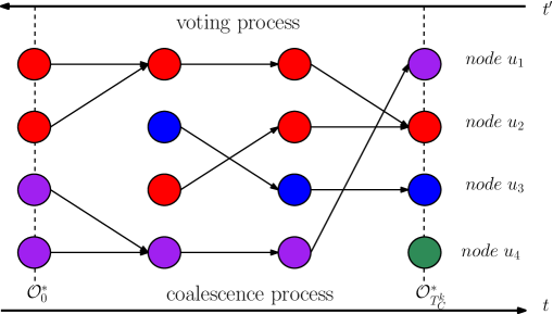
Figure 1: Running the coalescence process from right to left (an edge from $u$ to $v$ means that the token on $u$ -if any- moves to $v$) yields that after $T=4$ rounds the number of random walks reduces to $k=2$. Using the same random choices (black arrows) for the voter process and running the process from left to right (an edge from $u$ to $v$ means that $u$ pulls $v$’s opinion) we derive that the number of opinions after $T=4$ rounds is also $2$. This is no coincidence as we show in Lemma 4.

The following lemma uses the high-level idea of the proof presented in [AF02, Chapter 14] which only considers the case $k=1$. For the purposes of our proof we would only require a coupling with $T_{\mathcal{V}}^{k}\leq T_{C}^{k}$, but for the sake of completeness we show the stronger claim $T_{\mathcal{V}}^{k}=T_{C}^{k}$.

Lemma 4.

For any graph $G=(V,E)$, there exists a coupling such that $T_{C}^{k}=T_{\mathcal{V}}^{k}$.

Proof.

For $t\in\mathbb{N}$ and for $u\in V$ define the random variables $Y_{t}(u)$ with $Y_{t}(u)\sim\operatorname{uniform}(N(u))$, where $\operatorname{uniform}(\cdot)$ denotes the uniform distribution and $N(u)$ denotes the neighborhood of $u$. Hence, $Y_{t}(u)=v$ means that $u$ pulls information from node $v$ in step $t$. In the Coalescence process, the random variable $Y_{t}(u)\in N(u)$, $t\in[0,T_{C}^{k})$ captures the transition performed by the random walk which is at $u$ at time $t$ (if any). In other words, these random variables define the arrows in Figure 1. For the voter process $Y_{t}(u)=v$ means that in step $t$ node $u$ adopts the opinion of $v$.

Let $X(u)=(X_{0}(u)=u,X_{1}(u),\dots,X_{T_{C}^{k}}(u))$ be the trajectory of the random walk starting at $u$. We can thus express

$$X_{t}(u)=\begin{cases}u&\text{ if $t=0$}\\ Y_{t-1}(X_{t-1}(u))&\text{ otherwise.}\end{cases}$$ (10)

Thus, this trajectory $X(u)$ and the random variable $T_{C}^{k}$ are completely determined by the random variables $\mathcal{Y}=\{Y_{t}(u)\colon t\in\mathbb{N},u\in V\}$.

Let $\mathcal{V}_{T_{C}^{k}}$ be the Voter process whose starting time $t^{\prime}=0$ equals the time $T_{C}^{k}$ of the coalescence process (see also Figure 1). Let $\mathcal{O}^{*}_{T_{C}^{k}-t^{\prime}}(u)$ be the opinion of $u$ at time $t^{\prime}$ of $\mathcal{V}_{T_{C}^{k}}$. For every node $u\in V$ and $t^{\prime}\in[0,T_{C}^{k}]$ we can thus express

$$\mathcal{O}^{*}_{T_{C}^{k}-t^{\prime}}(u)=\begin{cases}u&\text{ if $t^{\prime}=0$}\\ \mathcal{O}^{*}_{T_{C}^{k}-(t^{\prime}-1)}(Y_{T_{C}^{k}-t^{\prime}}(u))&\text{ otherwise.}\end{cases}$$ (11)

Note that (11) constructs a coupling between the Voter process and the coalescence process through the common usage of the random variables $\mathcal{Y}$ in (10) and (11). In particular, by unrolling (10) and (11) we get

$$X_{T_{C}^{k}}(u) =Y_{T_{C}^{k}-1}(Y_{T_{C}^{k}-2}(\dots(Y_{0}(X_{0}(u)))\dots))\stackrel{{\scriptstyle(a)}}{{=}}Y_{T_{C}^{k}-1}(Y_{T_{C}^{k}-2}(\dots(Y_{0}(u))\dots))$$

$$O^{*}_{0}(u) =O^{*}_{T_{C}^{k}}(Y_{T_{C}^{k}-1}(Y_{T_{C}^{k}-2}(\dots(Y_{0}(u))\dots)))\stackrel{{\scriptstyle(b)}}{{=}}Y_{T_{C}^{k}-1}(Y_{T_{C}^{k}-2}(\dots(Y_{0}(u)\dots)),$$

where and $(a)$ we used that $X_{0}(u)=u$ and in $(b)$ we used that $O^{*}_{T_{C}^{k}}(v)=v$ for all $v$. The above equations imply

$$X_{T_{C}^{k}}(u)=\mathcal{O}^{*}_{0}(u).$$ (12)

Let $Z_{t}=\{X_{t}(u)\colon u\in V\}$ denote the positions of the remaining walks in the coalescence process at time $t$. Observe that $|Z_{0}|=n$, $|Z_{T_{C}^{k}}|\leq k$, by definition of $T_{C}^{k}$. We have, by (12), that

$$Z_{T_{C}^{k}}=\{X_{T_{C}^{k}}(u)\colon u\in V\}=\{\mathcal{O}^{*}_{0}(u)\colon u\in V\}=:\mathcal{O}^{*}_{0}.$$ (13)

From (13) we infer $|\mathcal{O}^{*}_{0}|=|Z_{T_{C}^{k}}|\leq k$, which implies that

$$T_{\mathcal{V}}^{k}\leq T_{C}^{k}.$$

In the reminder we generalize the previous coupling to show that

$$T_{\mathcal{V}}^{k}=T_{C}^{k}.$$

In particular, we consider the Voter process for all starting position $\tau<T_{C}^{k}$ (all nodes have different colors at round $t$) and show that the resulting number of opinions is strictly more than $k$.

Let $\mathcal{V}_{\tau}$ be the Voter process that starts at time $\tau\in[0,T_{C}^{k})$, and let $\mathcal{O}^{\tau}_{T_{C}^{k}-t^{\prime}}(u)$ be the opinion of $u$ at time $t^{\prime}$ of $\mathcal{V}_{\tau}$. For every node $u\in V$ and $t^{\prime}\in[0,\tau]$ we have

$$\mathcal{O}^{\tau}_{\tau-t^{\prime}}(u)=\begin{cases}u&\text{ if $t^{\prime}=\tau$}\\ \mathcal{O}^{\tau}_{\tau-(t^{\prime}-1)}(Y_{\tau-t^{\prime}}(u))&\text{ otherwise.}\end{cases}$$ (14)

Similarly as before, by unrolling (10) and (14) we get

$$X_{\tau}(u) =Y_{\tau-1}(Y_{\tau-2}(\dots(Y_{0}(X_{0}(u)))\dots))\stackrel{{\scriptstyle(a)}}{{=}}Y_{\tau-1}(Y_{\tau-2}(\dots(Y_{0}(u))\dots))$$

$$O^{\tau}_{0}(u) =O^{\tau}_{\tau}(Y_{\tau-1}(Y_{\tau-2}(\dots(Y_{0}(u))\dots)))\stackrel{{\scriptstyle(b)}}{{=}}Y_{\tau-1}(Y_{\tau-2}(\dots(Y_{0}(u)\dots)),$$

where and $(a)$ we used that $X_{0}(u)=u$ and in $(b)$ we used that $O^{\tau}_{\tau}(v)=v$ for all $v$. By defining $\mathcal{O}^{0}_{T_{C}^{k}-t^{\prime}}=\{\mathcal{O}^{0}_{T_{C}^{k}-t^{\prime}}(u)\colon u\in V\},$ from the above equations we get that

$$X_{\tau}(u)=\mathcal{O}^{\tau}_{0}(u).$$

Hence,

$$Z_{\tau}=\{X_{\tau}(u)\colon u\in V\}=\{\mathcal{O}^{\tau}_{0}(u)\colon u\in V\}=:\mathcal{O}^{\tau}_{0}.$$ (15)

Since for all $\tau<T_{C}^{k}$ we have $|Z_{\tau}|>k$, from (15) it follows that $|\mathcal{O}^{\tau}_{0}|=|Z_{\tau}|>k$ which yields the claim. ∎

A.6 Proof of Lemma 3

We prove the lemma using the well-known duality (via time reversal) between the Voter process and coalescing random walks.

It is well-known (e.g., [AF02]), that $T_{\mathcal{V}}^{1}=T_{C}^{1}$. This statement generalizes for all $k\in[n]$ (see Lemma 4 in Appendix A for a proof) to

$$T_{\mathcal{V}}^{k}=T_{C}^{k}.$$ (16)

Thanks to the previous identity, we can prove the lemma’s statement by proving that w.h.p. $T_{C}^{k}=\mathrm{O}\mathopen{}\mathclose{{}\left(\frac{n}{k}\log n}\right)$. To this end, we show that $\mathbb{E}\mathopen{}\mathclose{{}\left[{T_{C}^{k}}}\right]=\mathrm{O}\mathopen{}\mathclose{{}\left(n/k}\right)$. In order to get the claimed bound in concentration, we can apply the following standard argument. Consider the process as a sequence of phases, each one of length $2\mathbb{E}\mathopen{}\mathclose{{}\left[{T_{C}^{k}}}\right]$. We say that a phase is successful when the number of remaining random walks drops below $n/k$. Thanks to our bound in expectation above and the Markov inequality, we easily get that every phase has probability $\Omega(1)$ to be successful. So, with high probability, there will be at least one success within the first $\mathrm{O}\mathopen{}\mathclose{{}\left(\log n}\right)$ phases.

Let $X_{t}$ denote the number of coalescing random walks at time $t$. We have $X_{0}=n$ and $T_{C}^{k}=\min\set{t\geq 0}{X_{t}\leq k}$. We seek to apply drift theory (Theorem 7 in Appendix A.4) to derive a bound on $\mathbb{E}\mathopen{}\mathclose{{}\left[\,T_{C}^{k}\,}\right]$. Next, we compute an upper bound on $\mathbb{E}\mathopen{}\mathclose{{}\left[\,X_{t+1}-X_{t}\leavevmode\nobreak\ |\leavevmode\nobreak\ X_{t}=x\,}\right]$.

Let us begin assuming that $k$ is any constant. It holds in general that $\mathbb{E}\mathopen{}\mathclose{{}\left[\,X_{t+1}-X_{t}\mid X_{t}\geq 2\,}\right]\leq-1/n$, since in expectation two random walks collide w.p. $1/n$ in a given time step. Hence we can directly apply Theorem 7 with parameters $h(x)=1/n$ to reduce from $k$ random walks to $1$, yielding the bound $\mathbb{E}\mathopen{}\mathclose{{}\left[\,T_{C}^{k}\,}\right]=O(n/k)=O(n)$, where in the latter equality we used that $k$ is constant.

We now consider the case where $k$ is larger than a big constant, say $k>100$. Assume that in every time step the random walks move in two phases. Let $W_{1}$ denote an arbitrary set of $\lfloor X_{t}/2\rfloor$ random walks and let $W_{2}$ denote the remaining ones. We first look at how the random walks in $W_{1}$ coalesce, then we consider the movement of the remaining walks $W_{2}$. Let $\mathcal{E}$ be the event that the walks in $W_{1}$ move onto more than $\lfloor X_{t}/4\rfloor$ distinct nodes. This would imply that each walk in $W_{2}$ coalesces with one in $W_{1}$ with probability at least ${\lfloor X_{t}/4\rfloor}/{n}$. We thus have

$$\mathbb{E}\mathopen{}\mathclose{{}\left[\,X_{t+1}\leavevmode\nobreak\ |\leavevmode\nobreak\ X_{t}=x,\mathcal{E}\,}\right]\leq x-\lceil x/2\rceil\cdot\frac{\lfloor x/4\rfloor}{n}\leq x-\frac{x^{2}}{10n}.$$

Moreover, conditioning on $\overline{\mathcal{E}}$ implies that there were at least $\lfloor X_{t}/2\rfloor-\lfloor X_{t}/4\rfloor$ collisions during the first phase. Thus,

$$\mathbb{E}\mathopen{}\mathclose{{}\left[\,X_{t+1}\leavevmode\nobreak\ |\leavevmode\nobreak\ X_{t}=x,\overline{\mathcal{E}}\,}\right]\leq x-(\lfloor x/2\rfloor-\lfloor x/4\rfloor)\leq x-\frac{x^{2}}{10n}.$$

Hence, by law of total expectation,

$$\mathbb{E}\mathopen{}\mathclose{{}\left[\,X_{t+1}\leavevmode\nobreak\ |\leavevmode\nobreak\ X_{t}=x\,}\right] =\mathbb{E}\mathopen{}\mathclose{{}\left[\,X_{t+1}\leavevmode\nobreak\ |\leavevmode\nobreak\ X_{t}=x,\mathcal{E}\,}\right]\Pr\mathopen{}\mathclose{{}\left[{\mathcal{E}}}\right]+\mathbb{E}\mathopen{}\mathclose{{}\left[\,X_{t+1}\leavevmode\nobreak\ |\leavevmode\nobreak\ X_{t}=x,\overline{\mathcal{E}}\,}\right]\Pr\mathopen{}\mathclose{{}\left[{\overline{\mathcal{E}}}}\right]$$

$$\leq x-\frac{x^{2}}{10n}.$$

In order to apply Theorem 7, we define the random variables $(Y_{t})_{t\geq 0}$ as follows

$$Y_{t}=\begin{cases}X_{t}&\text{if $X_{t}>k$,}\\ 0&\text{otherwise.}\end{cases}$$

Let $T^{*}=\{t\geq 0\leavevmode\nobreak\ |\leavevmode\nobreak\ Y_{t}=0\}$. Since by construction we have $Y_{t}=X_{t}$ for $t<T_{C}^{k}$ and $Y_{T_{C}^{k}}=0$ otherwise, it follows that

$$T_{C}^{k}=T^{*}.$$ (17)

Therefore,

$$\mathbb{E}\mathopen{}\mathclose{{}\left[\,Y_{t+1}\leavevmode\nobreak\ |\leavevmode\nobreak\ Y_{t}=y,Y_{t}>k\,}\right]\leq y-\frac{y^{2}}{10n}.$$

We can thus apply Theorem 7 for the random variables $(Y_{t})_{t\geq 0}$ with $x_{\min}=k,x_{\max}=n$, and $h(x)=\frac{x^{2}}{10n}$, obtaining

$$\mathbb{E}\mathopen{}\mathclose{{}\left[\,T^{*}\,}\right] \leq\frac{k}{k^{2}/(10n)}+\int\limits_{k}^{n}\frac{1}{h(u)}\leq\frac{10n}{k}+10n\mathopen{}\mathclose{{}\left(-\frac{1}{n}-\mathopen{}\mathclose{{}\left(-\frac{1}{k}}\right)}\right)\leq 20\frac{n}{k}.$$ (18)

Finally, from (16), (17) and (18) we get

$$\mathbb{E}\mathopen{}\mathclose{{}\left[\,T_{\mathcal{V}}^{k}\,}\right]=\mathbb{E}\mathopen{}\mathclose{{}\left[\,T_{C}^{k}\,}\right]=\mathbb{E}\mathopen{}\mathclose{{}\left[\,T^{*}\,}\right]\leq 20\frac{n}{k},$$ (19)

concluding the proof. ∎

A.7 Proof of Theorem 4

Consider any initial configuration $c\in\mathcal{C}$. By applying Lemma 3 for $k=n^{1/4}$, we get that Voter reduces the number of remaining colors w.h.p. from initially at most $n$ to $n^{1/4}$ in $\mathrm{O}\bigl{(}n^{3/4}\log^{7/8}n\bigr{)}$ rounds. By Lemma 2, the time it takes $3$-Majority to reach some fixed number of remaining colors is dominated by the time it takes Voter to reach the same number of remaining colors. In particular, we get that $3$-Majority also reduces the number of remaining colors w.h.p. to $n^{1/4}$ in $\mathrm{O}\bigl{(}n^{3/4}\log^{7/8}n\bigr{)}$ rounds. That is, the first phase takes $\mathrm{O}\bigl{(}n^{3/4}\log^{7/8}n\bigr{)}$ rounds.

For the second phase, we apply [BCN⁺16, Theorem 3.1] (see Theorem 8 in Appendix A) for $k=n^{1/4}=\mathrm{o}\mathopen{}\mathclose{{}\left(n^{1/3}}\right)$. This immediately yields that the second phase takes $\mathrm{O}\bigl{(}n^{3/4}\log^{7/8}n\bigr{)}$ rounds, finishing the proof. ∎

A.8 Proof of Theorem 5

Let $T_{i}=\min\{t\geq 0\leavevmode\nobreak\ |\leavevmode\nobreak\ c_{i}(t)>\ell^{\prime}\}$. For any fixed opinion $i\leq k$ we show that $\Pr\mathopen{}\mathclose{{}\left[{T_{i}<n/(\gamma\ell^{\prime})}}\right]\leq 1/n^{2}$, so that, by a union bound over all opinions and using that $T=\min\{T_{i}\leavevmode\nobreak\ |\leavevmode\nobreak\ i\leq k\}$, we obtain $\Pr\mathopen{}\mathclose{{}\left[{T<n/(\gamma\ell^{\prime})}}\right]\leq 1/n$. Intuitively, we would like to show that, conditioning on $c_{i}\leq\ell^{\prime}$, the expected number of nodes joining opinion $i$ is dominated by a binomial distribution with parameters $n$ and $p=(\ell^{\prime}/n)^{2}$. The main obstacle to this is that naïvely applying Chernoff bounds for every time step yields a weak bound, since with constant probability at each round at least one color increases its support by a constant number of nodes. Instead, we consider a new process $\mathcal{P}$ in which the number $P(t)$ of nodes supporting color $i$ at time $t$ majorizes $c_{i}(t)$ as long as $P(t)\leq\ell^{\prime}$; we will then show that, after a certain time w.h.p. $P(t)$ is still smaller than $\ell^{\prime}$ implying that $\mathcal{P}$ indeed majorizes the original process. Using the fact that in $\mathcal{P}$ we can simply apply Chernoff bounds over several rounds, we can finally get $c_{i}\leq P(t)\leq\ell^{\prime}$ w.h.p..

Formally, process $\mathcal{P}$ is defined as follows. $P(0):=\ell$ and $P(t+1)=P(t)+\sum_{j\leq n}X_{j}^{(t)}$, where $X_{j}^{(t)}$ is a Bernoulli random variable with $\Pr\mathopen{}\mathclose{{}\left[{X_{i}=1}}\right]=p$ and, by a standard coupling, it is $1$ whenever node $j$ sees two times color $i$ at round $t$ (note that the latter event happens with probability at most $p$ for any $t<T_{i}$). By definition, if $t<T_{i}$ it holds $c_{i}(t)\leq\ell^{\prime}$, which implies that the probability that any node in the original process gets opinion $i$ is at most $p$. Thus, we can couple 2-Choices and $P$ for $t\leq T_{i}$ so that $c_{i}(t)\leq P(t)$. This implies that

$$T^{\prime}\coloneqq\min\{t\geq 0\leavevmode\nobreak\ |\leavevmode\nobreak\ P(t)\geq\ell^{\prime}\}\preceq T_{i}.$$ (20)

In the remainder we show that $\Pr\mathopen{}\mathclose{{}\left[{T^{\prime}<n/(\gamma\ell^{\prime})}}\right]<1/n^{2}$. For any round $t+1$, we define $\Delta_{t+1}\coloneqq P(t+1)-P(t)=\sum_{i\leq n}X_{i}$. Observe that $\Delta_{t+1}\sim\operatorname{Bin}(n,p)$. Let $t_{0}=n/(\gamma\ell^{\prime})$. In the following we bound

$$B\coloneqq P(t_{0})-P(0)=\sum_{i=1}^{t_{0}}\Delta_{i}.$$

Observe that $B\sim\operatorname{Bin}(t_{0}\cdot n,p)$ and thus $\mathbb{E}\mathopen{}\mathclose{{}\left[\,B\,}\right]=t_{0}\cdot n\cdot p$.

Using Chernoff bounds, e.g., [MU05, Theorem 4.4] we derive for any $\gamma\geq 18$

$$\Pr\mathopen{}\mathclose{{}\left[{P(t_{0})\geq\ell^{\prime}}}\right] =\Pr\mathopen{}\mathclose{{}\left[{B\geq\ell^{\prime}-\ell}}\right]\leq\Pr\mathopen{}\mathclose{{}\left[{B\geq\max\mathopen{}\mathclose{{}\left\{2\mathbb{E}\mathopen{}\mathclose{{}\left[\,B\,}\right],\frac{\gamma}{2}\log n}\right\}}}\right]$$

$$=\Pr\mathopen{}\mathclose{{}\left[{B\geq\mathbb{E}\mathopen{}\mathclose{{}\left[\,B\,}\right]\cdot\max\mathopen{}\mathclose{{}\left\{2,1+\frac{\frac{\gamma}{2}\log n}{\mathbb{E}\mathopen{}\mathclose{{}\left[\,B\,}\right]}}\right\}}}\right]\leq\exp\mathopen{}\mathclose{{}\left(-\frac{\frac{\gamma}{2}\log n}{3}}\right)\leq 1/n^{3},$$ (21)

where we used that

$$\max\mathopen{}\mathclose{{}\left\{2\mathbb{E}\mathopen{}\mathclose{{}\left[\,B\,}\right],\frac{\gamma}{2}\log n}\right\} =\max\mathopen{}\mathclose{{}\left\{2t_{0}\cdot n\cdot p,\frac{\gamma}{2}\log n}\right\}$$

$$\leq\max\mathopen{}\mathclose{{}\left\{\frac{(\ell^{\prime})^{2}}{\gamma\ell^{\prime}},\frac{\gamma}{2}\log n}\right\}$$

$$\leq\max\mathopen{}\mathclose{{}\left\{{\frac{\ell^{\prime}}{2}},\frac{\gamma}{2}\log n}\right\}$$

$$\leq\frac{\ell^{\prime}}{2}=\ell^{\prime}-\ell.$$

Putting everything together yields

$$\Pr\mathopen{}\mathclose{{}\left[{T<n/(\gamma\ell^{\prime})}}\right] =\Pr\mathopen{}\mathclose{{}\left[{T<t_{0}}}\right]$$ (22)

$$\stackrel{{\scriptstyle(a)}}{{\leq}}n\Pr\mathopen{}\mathclose{{}\left[{T_{i}<t_{0}}}\right]$$

$$\stackrel{{\scriptstyle(b)}}{{\leq}}n\Pr\mathopen{}\mathclose{{}\left[{T^{\prime}<t_{0}}}\right]$$

$$\stackrel{{\scriptstyle(c)}}{{\leq}}n\Pr\mathopen{}\mathclose{{}\left[{P(t_{0})\geq\ell^{\prime}}}\right]\stackrel{{\scriptstyle(d)}}{{\leq}}n^{-2},$$ (23)

where in $(a)$ we used union bound over all colors, in $(b)$ we used (20), in $(c)$ we used that “$T^{\prime}<t_{0}$”$\implies$ “$P(t_{0})\geq\ell^{\prime}$” and in $(d)$ we used (21). This completes the proof. ∎

Appendix B Limitations of Lemma 1

In this section we show that there are configurations $c\preceq\tilde{c}$ such that $\alpha^{(hM)}(c)\not\preceq\alpha^{(h+1M)}(\tilde{c})$. This means that, Lemma 1 is not strong enough to derive 1. Consider the configurations $x\coloneqq(1/2,1/6,1/6,1/6)\preceq(1/2,1/2,0,0)\eqqcolon\tilde{x}$ (for simplicity, we use the fraction vectors $x=c/n$). For symmetry reasons, we immediately get that $\alpha^{(h+1M)}(\tilde{c})=(1/2,1/2,0,0)=\tilde{c}$. However, even for $h=3$, for the second configuration we get that the expected fraction of the nodes which adopt the first opinion after one step is

$$1\cdot\binom{3}{0}\cdot{\mathopen{}\mathclose{{}\left(\frac{1}{2}}\right)}^{3}+1\cdot\binom{3}{1}\cdot{\mathopen{}\mathclose{{}\left(\frac{1}{2}}\right)}^{2}\cdot\frac{3}{6}+\frac{1}{3}\cdot\binom{3}{2}\cdot\frac{1}{2}\cdot\frac{3}{6}\cdot\frac{2}{6}=\frac{7}{12}.$$ (24)

The three terms of the sum on the left hand side correspond to the cases and probabilities for which the first color is adopted:

• all samples choose color $1$ (probability to win is $1$, number of cases $\binom{3}{0}$),

• two samples choose color $1$ (probability to win is $1$, number of cases $\binom{3}{1}$), or

• 1 sample chooses color $1$ and the other samples choose different colors (probability to win is $1/3$, number of cases $\binom{3}{2}$).

Thus, for $n$ large enough, with high probability the configuration resulting from $(h+1)$-Majority will not majorize the one resulting from h$-\textsc{Majority}$.

References

- [AF02] D. Aldous and J. Fill. Reversible markov chains and random walks on graphs, 2002. Unpublished. http://www.stat.berkeley.edu/~aldous/RWG/book.html.
- [BCN+14] Luca Becchetti, Andrea E. F. Clementi, Emanuele Natale, Francesco Pasquale, Riccardo Silvestri, and Luca Trevisan. Simple dynamics for plurality consensus. In 26th ACM Symposium on Parallelism in Algorithms and Architectures, (SPAA), pages 247–256, 2014.
- [BCN+15] Luca Becchetti, Andrea Clementi, Emanuele Natale, Francesco Pasquale, and Riccardo Silvestri. Plurality consensus in the gossip model. In Proceedings of the 26th Annual ACM-SIAM Symposium on Discrete Algorithms (SODA), pages 371–390, 2015.
- [BCN+16] Luca Becchetti, Andrea E. F. Clementi, Emanuele Natale, Francesco Pasquale, and Luca Trevisan. Stabilizing consensus with many opinions. In Proceedings of the Twenty-Sixth Annual ACM-SIAM Symposium on Discrete Algorithms (SODA). SIAM, 2016.
- [BFGK16] Petra Berenbrink, Tom Friedetzky, George Giakkoupis, and Peter Kling. Efficient plurality consensus, or: The benefits of cleaning up from time to time. In Proceedings of the 43rd International Colloquium on Automata, Languages and Programming (ICALP), 2016. to appear.
- [BG90] Carol Bezuidenhout and Geoffrey Grimmett. The critical contact process dies out. The Annals of Probability, pages 1462–1482, 1990.
- [BGKMT16] Petra Berenbrink, George Giakkoupis, Anne-Marie Kermarrec, and Frederik Mallmann-Trenn. Bounds on the voter model in dynamic networks. In ICALP, 2016.
- [BSDDS10] Ohad Ben-Shahar, Shlomi Dolev, Andrey Dolgin, and Michael Segal. Direction election in flocking swarms. In Proc. of the 6th Int. Workshop on Foundations of Mobile Computing (DIALM-POMC’10), pages 73–80. ACM, 2010.
- [CEOR13] Colin Cooper, Robert Elsässer, Hirotaka Ono, and Tomasz Radzik. Coalescing Random Walks and Voting on Connected Graphs. SIAM Journal on Discrete Mathematics, 27(4):1748–1758, 2013.
- [CER14] Colin Cooper, Robert Elsässer, and Tomasz Radzik. The power of two choices in distributed voting. In Automata, Languages, and Programming - 41st International Colloquium, (ICALP), pages 435–446, 2014.
- [CER+15] Colin Cooper, Robert Elsässer, Tomasz Radzik, Nicolas Rivera, and Takeharu Shiraga. Fast consensus for voting on general expander graphs. In Proceedings of the 29th International Symposium on Distributed Computing (DISC), 2015.
- [DGH+87] Alan Demers, Dan Greene, Carl Hauser, Wes Irish, John Larson, Scott Shenker, Howard Sturgis, Dan Swinehart, and Doug Terry. Epidemic algorithms for replicated database maintenance. In Proc. of the 6th Ann. ACM Symposium on Principles of Distributed Computing (PODC’12), pages 1–12. ACM, 1987.
- [DGM+11] Benjamin Doerr, Leslie Ann Goldberg, Lorenz Minder, Thomas Sauerwald, and Christian Scheideler. Stabilizing consensus with the power of two choices. In Proceedings of the 23rd Annual ACM Symposium on Parallelism in Algorithms and Architectures, (SPAA), pages 149–158, 2011.
- [DGRS14] Josep Díaz, Leslie Ann Goldberg, David Richerby, and Maria Serna. Absorption Time of the Moran Process. In Approximation, Randomization, and Combinatorial Optimization. Algorithms and Techniques (APPROX/RANDOM 2014), volume 28, pages 630–642, 2014.
- [EFK+16] Robert Elsässer, Tom Friedetzky, Dominik Kaaser, Frederik Mallmann-Trenn, and Horst Trinker. Efficient k-party voting with two choices. CoRR, abs/1602.04667, 2016.
- [FPM+02] Nigel R. Franks, Stephen C. Pratt, Eamonn B. Mallon, Nicholas F. Britton, and David J.T. Sumpter. Information flow, opinion polling and collective intelligence in house–hunting social insects. Philosophical Transactions of the Royal Society of London B: Biological Sciences, 357(1427):1567–1583, 2002.
- [GP16] Mohsen Ghaffari and Merav Parter. A polylogarithmic gossip algorithm for plurality consensus. In Proceedings of the 2016 ACM Symposium on Principles of Distributed Computing, pages 117–126. ACM, 2016.
- [HP01] Y. Hassin and D. Peleg. Distributed probabilistic polling and applications to proportionate agreement. Information and Computation, 171(2):248–268, 2001.
- [KDG03] David Kempe, Alin Dobra, and Johannes Gehrke. Gossip-Based Computation of Aggregate Information. In Proc. of 43rd Ann. IEEE Symp. on Foundations of Computer Science (FOCS’03), pages 482–491. IEEE, 2003.
- [KSSV00] Richard Karp, Christian Schindelhauer, Scott Shenker, and Berthold Vocking. Randomized rumor spreading. In Proc. of the 41th Ann. IEEE Symp. on Foundations of Computer Science (FOCS’00), pages 565–574. IEEE, 2000.
- [LHN05] E. Lieberman, C. Hauert, and M. Nowak. Evolutionary dynamics on graphs. Nature, 433(7023):312–316, January 2005.
- [Lig99] Thomas M Liggett. Stochastic interacting systems: contact, voter and exclusion processes. Springer, 2099.
- [LW14] Per Kristian Lehre and Carsten Witt. Concentrated hitting times of randomized search heuristics with variable drift. In Proceedings of the 25th International Symposium on Algorithms and Computation (ISAAC), pages 686–697, 2014.
- [MOA11] Albert W. Marshall, Ingram Olkin, and Barry C. Arnold. Inequalities: Theory of Majorization and Its Applications. Springer Series in Statistics. Springer, 2011.
- [Mor16] Satoru Morita. Six susceptible-infected-susceptible models on scale-free networks. Scientific reports, 6, 2016.
- [MU05] Michael Mitzenmacher and Eli Upfal. Probability and Computing: Randomized Algorithms and Probabilistic Analysis. Cambridge University Press, 2005.
- [PSL80] Marshall Pease, Robert Shostak, and Leslie Lamport. Reaching agreement in the presence of faults. Journal of the ACM, 27(2):228–234, 1980.
- [Rab83] Michael O. Rabin. Randomized byzantine generals. In Proc. of the 24th Ann. Symp. on Foundations of Computer Science (SFCS’83), pages 403–409. IEEE, 1983.
- [RS+77] Yosef Rinott, Thomas J Santner, et al. An inequality for multivariate normal probabilities with application to a design problem. The Annals of Statistics, 5(6):1228–1234, 1977.