Scaling limit of the uniform prudent walk

Abstract

We study the 2-dimensional uniform prudent self-avoiding walk, which assigns equal probability to all nearest-neighbor self-avoiding paths of a fixed length that respect the prudent condition, namely, the path cannot take any step in the direction of a previously visited site. The uniform prudent walk has been investigated with combinatorial techniques in Bousquet-Mélou (2010), while another variant, the kinetic prudent walk has been analyzed in detail in Beffara, Friedli and Velenik (2010). In this paper, we prove that the $2$-dimensional uniform prudent walk is ballistic and follows one of the $4$ diagonals with equal probability. We also establish a functional central limit theorem for the fluctuations of the path around the diagonal.

1 Introduction

The prudent walk was introduced in Turban and Debierre (1987a, b) and Santra, Seitz and Klein (2001) as a simplified version of the self-avoiding walk. It has attracted the attention of the combinatorics community in recent years, see e.g., Bousquet-Mélou (2010); Beaton and Iliev (2015); Dethridge and Guttmann , and also the probability community, see e.g. Beffara, Friedli and Velenik (2010) and Pétrélis and Torri (2016) .

In dimension $2$, for a given $L\in\mathbb{N}$, the set $\Omega_{L}$ of $L$-step prudent path on $\mathbb{Z}^{2}$ contains all nearest-neighbor self-avoiding path starting from the origin, which never take any step in the direction of a site already visited, i.e.,

$$\Omega_{L}:=\big{\{}(\pi_{i})_{i=0}^{L}\in(\mathbb{Z}^{2})^{L+1}\colon\, \pi_{0}=(0,0),\pi_{i+1}-\pi_{i}\in\{\leftarrow,\rightarrow,\downarrow,\uparrow\}\quad\forall i\in\{0,\dots,L-1\},$$

$$\big{(}\pi_{i}+\mathbb{N}(\pi_{i+1}-\pi_{i})\big{)}\cap\pi_{[0,i]}=\emptyset\quad\,\forall i\in\{0,\dots,L-1\}\big{\}}$$ (1.1)

where $\pi_{[0,i]}$ is the range of $\pi$ at time $i$, i.e., $\pi_{[0,i]}=\{\pi_{j}:0\leq j\leq i\}$.

Two natural laws can be considered on $\Omega_{L}$:

1. The uniform law $\boldsymbol{\mathrm{P}}_{\text{unif},L}$, also referred to as the uniform prudent walk, under which at every path in $\Omega_{L}$ is assigned equal probability $1/|\Omega_{L}|$;

2. The kinetic law $\boldsymbol{\mathrm{P}}_{\text{kin},L}$, also referred to as the kinetic prudent walk, under which each step of the path is chosen uniformly among all the admissible steps. Note that the first step is in one of the $4$ directions with equal probability. Subsequently, if a step increases either the width or the height of its range, then the next step has $3$ admissible choices; otherwise there are only $2$ admissible choices. Let ${\mathcal{H}}(\pi_{[0,L-1]})$ and ${\mathcal{W}}(\pi_{[0,L-1]})$ denote the height and width of the range of $\pi_{[0,L-1]}$. Then, for $L\in\mathbb{N}$ and $\pi\in\Omega_{L}$, we note that

   $$\boldsymbol{\mathrm{P}}_{\text{kin},L}(\pi) =\tfrac{1}{4}\big{(}\tfrac{1}{2}\big{)}^{L-{\mathcal{H}}(\pi_{[0,L-1]})-{\mathcal{W}}(\pi_{[0,L-1]})}\,\big{(}\tfrac{1}{3}\big{)}^{{\mathcal{H}}(\pi_{[0,L-1]})+{\mathcal{W}}(\pi_{[0,L-1]})}.$$ (1.2)

Beffara, Friedli and Velenik (2010) proved that the scaling limit of the kinetic prudent walk is given by $Z_{u}=\int_{0}^{3u/7}\big{(}\sigma_{1}{\sf 1}_{\{W_{s}\geq 0\}}{1\choose 0}+\sigma_{2}{\sf 1}_{\{W_{s}<0\}}{0\choose 1}\big{)}\text{\rm d}s$, where $W$ is a Brownian motion and $\sigma_{1},\sigma_{2}\in\{-1,1\}$ are random signs (independent of $W$), cf. (Beffara, Friedli and Velenik, 2010, Theorem 1).

In this paper, we identify rigorously the scaling limit of the 2-dimensional uniform prudent walk, proving a conjecture raised in several papers, e.g., (Beffara, Friedli and Velenik, 2010, Section 5), and (Bousquet-Mélou, 2010, Proposition 8) where partial answers were provided for the 2-sided and 3-sided versions of the 2-dimensional prudent walk using combinatorial techniques. The conjecture, supported by numerical simulations, was that when space and time are rescaled by the length $L$, the 2-dimensional uniform prudent walk converges to a straight line in one of the 4 diagonal directions chosen with equal probability. This is in stark contrast to the kinetic prudent walk.

2 Main results

Definition 2.1.

For every $\pi\in\Omega_{L}$, let $\widetilde{\pi}^{L}:[0,1]\mapsto\mathbb{R}^{2}$ be the rescaled and interpolated version of $\pi$, i.e.,

$$\widetilde{\pi}^{L}_{t}=\frac{1}{L}\big{(}\pi_{\lfloor tL\rfloor}+(tL-\lfloor tL\rfloor)(\pi_{\lfloor tL\rfloor+1}-\pi_{\lfloor tL\rfloor})\big{)},\quad t\in[0,1].$$

We also denote $\vec{e}_{1}:=(1,1)$, $\vec{e}_{2}:=(-1,1)$, $\vec{e}_{3}:=(-1,-1)$ and $\vec{e}_{4}:=(1,-1)$.

Our first result shows that the scaling limit of the uniform prudent walk is a straight line segment.

Theorem 2.2 (Concentration along the diagonals).

There exists a $c>0$ such that for every $\varepsilon>0$

$$\lim_{L\to\infty}\boldsymbol{\mathrm{P}}_{{\rm unif},L}\bigg{(}\exists\,i\in\{1,\dots,4\}\ s.t.\ \sup_{t\in[0,1]}\big{|}\widetilde{\pi}^{L}_{t}-ct\,\vec{e}_{i}\big{|}\leq\varepsilon\bigg{)}=1.$$ (2.1)

Furthermore, we can identify the fluctuation of the prudent walk around the diagonal. More precisely, let $\sigma_{L}=1,2,3,4$, depending on whether $\widetilde{\pi}^{L}_{1}$ lies in the interior of the 1st, 2nd, 3rd, or the 4th quadrant, and let $\sigma_{L}=0$ otherwise. Then we have

Theorem 2.3 (Fluctuations around the diagonal).

Under $\boldsymbol{\mathrm{P}}_{{\rm unif},L}$, the law of $\sigma_{L}$ converges to the uniform distribution on $\{1,2,3,4\}$, and

$$\big{(}\sqrt{L}(\widetilde{\pi}^{L}_{t}-ct\vec{e}_{\sigma_{L}})\big{)}_{t\in[0,1]}\Rightarrow(B_{t})_{t\in[0,1]}\qquad\mbox{as }L\to\infty,$$ (2.2)

where $\Rightarrow$ denotes weak convergence, and $(B_{t})_{t\geq 0}$ is a two-dimensional Brownian motion with a non-degenerate covariance matrix, cf. (3.28).

The proof of Theorem 2.2 follows the strategy used by Beffara, Friedli and Velenik (2010). We consider the so called uniform 2-sided prudent walk (cf. Section 3), a sub-family of prudent walks with a fixed diagonal direction. First we prove that the scaling limit of the uniform 2-sided prudent walk is a straight line, cf. Theorem 3.1. A weaker version of this result was already proven by (Bousquet-Mélou, 2010, Proposition 6). We reinforce it by using an alternative probabilistic approach. We decompose a path into a sequence of excursions, which leads to an effective one-dimensional random walk with geometrical increments, see e.g., Figure 1. Then we show that under the uniform measure, a typical path of length $L$ crosses its range from one end to the other at most $\log L$ times and the total length of the first $\log L$ excursions also grows at most logarithmically in $L$. This results refines the upper bound obtained by Pétrélis and Torri (2016). The excursions crossing the range of the walk disappear in the scaling limit, while the remaining part of the path is nothing but a uniform 2-sided prudent walk (in one of the four diagonal directions), for which we have identified the correct scaling limit.

Theorem 2.3 can be proved using the same strategy. Once it is shown to hold for the 2-sided uniform prudent walk, cf. Theorem 3.2, then it also holds for the uniform prudent walk thanks to control on the number of excursions crossing the range of the walk.

2.1 Organization of the paper

The article is organized as follows: In Section 3, we introduce the uniform 2-sided prudent walk and identify its scaling limit. In Section 4, we analyze the uniform prudent walk and prove some technical results needed to control the excursions crossing the range of the walk. Lastly, we prove our main results Theorems 2.2 and 2.3 in Section 5.

3 Uniform 2-sided prudent walk

Let $\Omega_{L}^{+}$ be the subset of $\Omega_{L}$ containing the so called 2-sided prudent path (in the north-east direction), that is, those paths $\pi\in\Omega_{L}$ satisfying three additional geometric constraints:

1. $\pi$ can not take any step in the direction of any site in the quadrant $(-\infty,0]^{2}$;

2. The endpoint $\pi_{L}$ is located at the top-right corner of the smallest rectangle containing $\pi$;

3. $\pi$ starts with an east step ($\rightarrow$), i.e., $\pi_{1}=(1,0)$.

We denote by $\boldsymbol{\mathrm{P}}_{\text{unif},L}^{+}$ the uniform measure on $\Omega_{L}^{+}$. Theorems 3.1 and 3.2 below are the counterparts of Theorems 2.2 and 2.3 for the uniform 2-sided prudent walk. Recall that $\vec{e}_{1}=(1,1)$.

Theorem 3.1.

There exists a $c>0$ such that for every $\varepsilon>0$,

$$\lim_{L\to\infty}\boldsymbol{\mathrm{P}}_{{\rm unif},L}^{+}\bigg{(}\sup_{t\in[0,1]}\big{|}\widetilde{\pi}^{L}_{t}-ct\,\vec{e}_{1}\big{|}\leq\varepsilon\bigg{)}=1.$$ (3.1)

Theorem 3.2.

Under $\boldsymbol{\mathrm{P}}^{+}_{{\rm unif},L}$,

$$\big{(}\sqrt{L}(\widetilde{\pi}^{L}_{t}-ct\vec{e}_{1})\big{)}_{t\in[0,1]}\Rightarrow(B_{t})_{t\in[0,1]}\qquad\mbox{as }L\to\infty.$$ (3.2)

where $B$ is the same two-dimensional Brownian motion as in Theorem 2.3.

3.1 Decomposition of a 2-sided prudent path into excursions

Every path $\pi\in\Omega_{L}^{+}$ can be decomposed in a unique manner into a sequence of horizontal and vertical excursions (see Figure 1). First we introduce some notation. For $\pi\in\Omega_{L}^{+}$ and $i\leq L$, denote $\pi_{i}=(\pi_{i,1},\pi_{i,2})$. Let $\tau_{0}:=0$ and

$$\tau_{1}(\pi):=\min\{i>0\,:\,\pi_{i,2}>0\}-1, \tau_{2}(\pi):=\min\{i>\tau_{1}\,:\,\pi_{i,1}>\pi_{\tau_{1,1}}\}-1,$$ (3.3)

which are the times when the first horizontal, resp.  vertical excursion ends. For $k\in\mathbb{N}$, define

$$\tau_{2k+1}(\pi):=\inf\{i>\tau_{2k}\,:\,\pi_{i,2}>\pi_{\tau_{2k,2}}\}-1, \tau_{2k+2}(\pi):=\inf\{i>\tau_{2k+1}\,:\,\pi_{i,1}>\pi_{\tau_{2k+1,1}}\}-1.$$

Let $\gamma_{L}(\pi):=\min\{j\geq 1\colon\,\tau_{j}(\pi)=\infty\}$ be the number of excursions in $\pi$. Note that each horizontal excursion starts with an east step, and each vertical excursion a north step. Since the endpoint $\pi_{L}$ lies at the top-right corner of the smallest rectangle containing $\pi$, the last excursion of $\pi$ can be made complete by adding an extra north step if it is a horizontal excursion, or adding an extra east step if it is a vertical excursion. Therefore, with a slight abuse of notation, we redefine $\tau_{\gamma_{L}}:=L$. We can thus decompose $\pi$ into the excursions $\big{(}(\pi_{\tau_{k-1}},\dots,\pi_{\tau_{k}})\big{)}_{k=1}^{\gamma_{L}}$, which are horizontal for odd $k$ and vertical for even $k$.

3.2 Effective random walk excursion

Let ${\mathcal{I}}_{t}$ denote the set of horizontal excursions of length $t$, flipped above the $x$-axis, i.e.,

$${\mathcal{I}}_{t}:=\big{\{}\pi=(\pi_{0},\pi_{1},\dots,\pi_{t})\colon\pi_{0}=(0,0),\,\pi_{1}=(1,0),\ \pi_{i,2}\geq 0\ \forall\,i\in\{1,\dots,t\},\,\pi_{t,2}=0\big{\}}.$$ (3.4)

Recall from Section 3.1 that each path $\pi\in\Omega_{L}^{+}$ can be decomposed uniquely into $\gamma_{L}(\pi)$ excursions of length $\tau_{i}-\tau_{i-1}$, $i=1,\dots,\tau_{L}(\pi)$. These excursions are alternatingly horizontal and vertical, with the first excursion being horizontal, see Figure 1. We can thus partition $\Omega_{L}^{+}$ according to the value of $r:=\gamma_{L}(\pi)$ and the excursion lengths $t_{1},\dots,t_{r}$. Defining

$$K(t):=\frac{1}{2^{t}}\big{|}{\mathcal{I}}_{t}\big{|},$$ (3.5)

we have that

$$\frac{1}{2^{L}}\,|\Omega_{L}^{+}|=\sum_{r\geq 1}\sum_{t_{1}+\dots+t_{r}=L}\prod_{i=1}^{r}\Big{|}{\mathcal{I}}_{t_{i}}\Big{|}\,\frac{1}{2^{t_{i}}}=\sum_{r\geq 1}\sum_{t_{1}+\dots+t_{r}=L}\prod_{i=1}^{r}K(t_{i}).$$ (3.6)

We now follow the idea introduced in Beffara, Friedli and Velenik (2010) and rewrite (3.5) in terms of a one-dimensional effective random walk $V=(V_{i})_{i=0}^{\infty}$. The walk $V$ starts from $0$, has law $\mathbf{P}$, and its increments $(U_{i})_{i=0}^{\infty}$ are i.i.d. and follow a discrete Laplace distribution, i.e.,

$$\mathbf{P}(U_{1}=x)=\frac{1}{3}\,\frac{1}{2^{|x|}},\quad x\in\mathbb{Z}.$$ (3.7)

Lemma 3.3.

Given the walk $V$ and $t\in\mathbb{N}$, let $\eta_{t}:=\min\big{\{}i\geq 1\colon\,i+\sum_{j=1}^{i}|U_{j}|\geq t\big{\}}$, then

$$K(t)=\mathbf{E}\Big{[}e^{\log(\frac{3}{2})\,\eta_{t}}\,{\sf 1}_{\{V_{i}\geq 0\ \forall i\leq\eta_{t},\,V_{\eta_{t}=0},\ \eta_{t}+\sum_{j=1}^{\eta_{t}}|U_{j}|=t\}}\Big{]}.$$ (3.8)

Proof.

For each $\pi\in{\mathcal{I}}_{t}$ (cf. (3.4)), let $n(\pi):=|\pi_{t,1}-\pi_{0,1}|$ be the number of horizontal steps. Each horizontal step is followed by a stretch of vertical steps, and for $1\leq i\leq n$, let $\ell_{i}\in\mathbb{Z}$ denote the vertical displacement after the $i$-th horizontal step. This gives a bijection between ${\mathcal{I}}_{t}$ and $\bigcup_{n=1}^{t}{\mathcal{L}}_{n,t}$, where

$${\mathcal{L}}_{n,t}:=\bigg{\{}\underline{\ell}=(\ell_{1},\dots,\ell_{n})\in\mathbb{Z}^{n}\colon\sum_{k=1}^{j}\ell_{k}\geq 0\,\,\forall\,j=1,\dots,n,\,\sum_{k=1}^{n}\ell_{k}=0,\,n+\sum_{j=1}^{n}|\ell_{j}|=t\bigg{\}}.$$ (3.9)

At this stage we note that

$$\frac{1}{2^{t}}\big{|}{\mathcal{I}}_{t}\big{|}=\sum_{\pi\in{\mathcal{I}}_{t}}\frac{1}{2^{t-n(\pi)}}\frac{1}{3^{n(\pi)}}\,\Big{(}\frac{3}{2}\Big{)}^{n(\pi)}=\sum_{n=1}^{t}\sum_{\underline{\ell}\in{\mathcal{L}}_{n,t}}\frac{1}{3^{n}}\frac{1}{2^{\sum_{j=1}^{n}|\ell_{j}|}}e^{n\,\log(\frac{3}{2})}.$$ (3.10)

By identifying $\underline{\ell}=(\ell_{1},\dots,\ell_{n})$ in (3.10) with the increments of $V$, we get (3.8). ∎

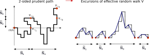
Figure 1: We decompose a path $\pi\in\Omega_{L}^{+}$ into a sequence of horizontal and vertical excursions $\big{(}(\pi_{\tau_{k-1}},\dots,\pi_{\tau_{k}})\big{)}_{k=1}^{4}$, each associated with an effective one dimensional random walk excursion.

3.3 Representation of the law of a uniform 2-sided prudent walk

Lemma 3.4.

Let $K$ be as in (3.8), then there exists $\lambda^{*}>0$ such that $\widehat{K}(\lambda^{*}):=\sum_{t=1}^{\infty}K(t)e^{-\lambda^{*}t}=1$.

Remark 3.5.

We will denote by $K^{*}$ the probability measure on $\mathbb{N}$ defined by

$$K^{*}(t)=K(t)e^{-\lambda^{*}t},\qquad t\in\mathbb{N}.$$ (3.11)

The proof of Lemma 3.4 below shows that there exists $\hat{\lambda}<\lambda^{*}$ such that $1<\widehat{K}(\hat{\lambda})<\infty$. Therefore $K^{*}$ has exponential tail, i.e., there exist $c_{1},c_{2}>0$ such that $K^{*}(n)\leq c_{1}e^{-c_{2}n}$ for every $n\in\mathbb{N}$.

The proof of Lemma 3.4 will be given at the end of the present section. We first explain how the law $K^{*}$ can be used to express the law $\boldsymbol{\mathrm{P}}^{*}$ of the excursions of the uniform two-sided prudent walk. Continuing Section 3.2, let ${\mathcal{V}}_{\infty}$ be the set of all non-negative excursions of the effective walk, i.e.,

$${\mathcal{V}}_{\infty}:=\bigcup_{N\geq 1}\Big{\{}(V_{i})_{i=0}^{N}\colon\,V_{0}=0,V_{i}\geq 0\ \forall i\leq N,\,V_{N}=0\Big{\}}.$$ (3.12)

By (3.8) and Lemma 3.4, we obtain the following probability law $\boldsymbol{\mathrm{P}}^{*}$ on ${\mathcal{V}}_{\infty}$, with Radon-Nikodym derivative

$$\frac{\text{\rm d}\boldsymbol{\mathrm{P}}^{*}}{\text{\rm d}\boldsymbol{\mathrm{P}}}\big{(}(V_{i})_{i=0}^{N}\big{)}=e^{\log(\frac{3}{2})N-\lambda^{*}(N+\sum_{i=1}^{N}|U_{i}|)}.$$ (3.13)

We will show that $\boldsymbol{\mathrm{P}}^{*}$ is in fact the law of a uniform 2-sided prudent walk excursion. To that end, consider a sequence $(t_{i},n_{i})_{i=1}^{r}\in\mathbb{N}^{r}\times\mathbb{N}^{r}$ satisfying $t_{1}+\dots+t_{r}=L$ and $n_{i}\leq t_{i}$ for every $i\leq r$. Let $\Omega_{L}^{+}\big{(}(t_{i},n_{i})_{i=1}^{r}\big{)}$ denote the set of 2-sided prudent path consisting of $r$ excursions, where the $i$-th excursion has total length $t_{i}$, with $n_{i}$ horizontal (resp. vertical) steps if it is a horizontal (resp. vertical) excursion. By the reasoning leading to (3.6), with $\alpha^{*}:=\log(3/2)-\lambda^{*}$, we obtain

$$\frac{1}{2^{L}}|\Omega_{L}^{+}\big{(}(t_{i},n_{i})_{i=1}^{r}\big{)}|e^{-\lambda^{*}L}=\prod_{i=1}^{r}\boldsymbol{\mathrm{E}}\bigg{[}e^{\alpha^{*}n_{i}-\lambda^{*}(t_{i}-n_{i})}\,{\sf 1}_{\big{\{}V_{j}\geq 0\,\forall j\leq n_{i},\,V_{n_{i}}=0,\,n_{i}+\sum_{j=1}^{n_{i}}|U_{j}|=t_{i}\big{\}}}\bigg{]}.$$ (3.14)

If $(\widetilde{T}_{i},\widetilde{N}_{i})_{i\in\mathbb{N}}$ denotes an i.i.d. sequence such that $\widetilde{N}_{1}=N$ and $\widetilde{T}_{1}=N+\sum_{i=1}^{N}|U_{i}|$ for a random walk excursion $(V_{i})_{i=0}^{N}$ following the law $\boldsymbol{\mathrm{P}}^{*}$ in (3.13), and

$$\widetilde{\gamma}_{L}:=\min\{i\geq 1\,:\,\widetilde{T}_{1}+\dots+\widetilde{T}_{i}\geq L\},$$ (3.15)

then by (3.6) and (3.14), for any set of paths $A$ which is a union of some $\Omega_{L}^{+}\big{(}(t_{i},n_{i})_{i=1}^{r}\big{)}$, we have

$$\boldsymbol{\mathrm{P}}_{\text{unif},L}^{+}(A)=\frac{|\Omega_{L}^{+}(A)|}{|\Omega_{L}^{+}|}=\frac{\boldsymbol{\mathrm{E}}^{*}\bigg{[}{\sf 1}_{A}{\sf 1}_{\{\widetilde{T}_{1}+\dots+\widetilde{T}_{\widetilde{\gamma}_{L}}=L\}}\bigg{]}}{\boldsymbol{\mathrm{P}}^{*}\bigg{[}\widetilde{T}_{1}+\dots+\widetilde{T}_{\widetilde{\gamma}_{L}}=L\bigg{]}},$$ (3.16)

where we also used $\boldsymbol{\mathrm{P}}^{*}$ to denote the joint law of the i.i.d. sequence of effective random walk excursions that give rise to $(\widetilde{T}_{i},\widetilde{N}_{i})_{i\in\mathbb{N}}$. This representation will be the basis of our analysis.

Proof of Lemma 3.4.

The existence of $\lambda^{*}$ is guaranteed if $\lambda^{**}:=\inf\{\lambda>0\colon\,\widehat{K}(\lambda)<\infty\}$ satisfies $\widehat{K}(\lambda^{**})>1$. To show this, let $\tau$ be the first time the walk $V$ returns to or crosses the origin, i.e.,

$$\tau=\begin{dcases*}1&if $V_{1}=0$,\\ \min\{i\geq 2\colon\,V_{i-1}V_{i}\leq 0\}&otherwise.\end{dcases*}$$ (3.17)

Let $\alpha:=\log(3/2)-\lambda$. By (3.8) and decomposing $V\in{\mathcal{V}}_{\infty}$ into positive excursions, we can write

$$\widehat{K}(\lambda) =\sum_{t\geq 1}\boldsymbol{\mathrm{E}}\Big{[}e^{(\log(\frac{3}{2})-\lambda)\eta_{t}-\lambda(t-\eta_{t})}\,{\sf 1}_{\{V_{i}\geq 0\ \forall i\leq\eta_{t},V_{\eta_{t}=0},\,\eta_{t}+\sum_{i=1}^{\eta_{t}}|U_{i}|=t\}}\Big{]}$$

$$=\sum_{t\geq 1}\sum_{N\leq t}\boldsymbol{\mathrm{E}}\Big{[}e^{\alpha N-\lambda(t-N)}\,{\sf 1}_{\{V_{i}\geq 0\ \forall i\leq N,\,V_{N}=0,\,N+\sum_{i=1}^{N}|U_{i}|=t\}}\Big{]}$$

$$=\sum_{N=1}^{\infty}\boldsymbol{\mathrm{E}}\Big{[}e^{\alpha N}\,e^{-\lambda\sum_{i=1}^{N}|U_{i}|}{\sf 1}_{\{V_{i}\geq 0\ \forall i\leq N,\,V_{N}=0\}}\Big{]}$$

$$=\sum_{N=1}^{\infty}\sum_{r=1}^{\infty}\sum_{n_{1}+\dots+n_{r}=N}\prod_{i=1}^{r}\boldsymbol{\mathrm{E}}\Big{[}e^{\alpha\tau}\,e^{-\lambda\sum_{i=1}^{\tau}|U_{i}|}\,{\sf 1}_{\{V_{1}\geq 0,\,\tau=n_{i},\,V_{n_{i}}=0\}}\Big{]}$$

$$=\sum_{r=1}^{\infty}\Big{(}\sum_{n=1}^{\infty}\boldsymbol{\mathrm{E}}\Big{[}e^{\alpha\tau-\lambda\sum_{i=1}^{\tau}|U_{i}|}\,{\sf 1}_{\{V_{1}\geq 0,\,\tau=n,\,V_{\tau}=0\}}\Big{]}\Big{)}^{r}$$

$$=\sum_{r=1}^{\infty}\left(\boldsymbol{\mathrm{E}}\Big{[}e^{\alpha\tau-\lambda\sum_{i=1}^{\tau}|U_{i}|}\,{\sf 1}_{\{V_{1}\geq 0,V_{\tau}=0\}}\Big{]}\right)^{r}=:\sum_{r=1}^{\infty}G(\lambda)^{r}.$$ (3.18)

Therefore $\lambda^{**}=\inf\{\lambda>0\colon\,G(\lambda)<1\}$, and it suffices to show that $G(\lambda^{**})>1/2$. Note that

$$\boldsymbol{\mathrm{E}}\Big{[}e^{\alpha\tau-\lambda\sum_{i=1}^{\tau}|U_{i}|}\,{\sf 1}_{\{V_{1}=0\}}\Big{]}=\frac{e^{\alpha}}{3},$$ (3.19)

and

$$\boldsymbol{\mathrm{E}}\Big{[}e^{\alpha\tau-\lambda\sum_{i=1}^{\tau}|U_{i}|}\,{\sf 1}_{\{V_{1}>0,\tau=n\}}\Big{]}=\boldsymbol{\mathrm{E}}\Big{[}e^{\alpha\tau-\lambda\sum_{i=1}^{\tau}|U_{i}|}\,{\sf 1}_{\{V_{1}>0,\tau=n,V_{\tau}=0\}}\Big{]}\frac{1}{1-e^{-\lambda}/2},$$ (3.20)

because given $(V_{i})_{i=0}^{n-1}$ with $V_{1}>0$, the events $\{\tau=n,V_{n}=0\}$ and $\{\tau=n\}$ differ only in that the first event requires $U_{n}=-V_{n-1}$, while the second event requires $U_{n}\leq-V_{n-1}$, and the probability ratio of the two events is precisely $\sum_{k=0}^{\infty}\frac{e^{-k\alpha}}{2^{k}}=\frac{1}{1-e^{-\lambda}/2}$ by (3.7). Summing over $n$ in (3.20), using the symmetry of $V$ and (3.19) then gives

$$G(\lambda) =\frac{e^{\alpha}}{3}\Big{(}\frac{1}{2}+\frac{e^{-\lambda}}{4}\Big{)}+\frac{1}{2}\Big{(}1-\frac{e^{-\lambda}}{2}\Big{)}\boldsymbol{\mathrm{E}}\Big{[}e^{\alpha\tau-\lambda\sum_{i=1}^{\tau}|U_{i}|}\Big{]}.$$ (3.21)

Now let $\hat{\lambda}$ be the unique solution of

$$\log\boldsymbol{\mathrm{E}}[e^{-\lambda|U_{1}|}]=-\alpha=\lambda-\log(3/2),\qquad\lambda\in[0,\infty).$$

Then $(M_{n}^{\hat{\lambda}})_{n\geq 0}:=(e^{\alpha n-\hat{\lambda}\sum_{i=1}^{n}|U_{i}|})_{n\geq 0}$ is a positive martingale. We will show that $\boldsymbol{\mathrm{E}}[M_{\tau}^{\hat{\lambda}}]=1$, which then gives $G(\hat{\lambda})=\frac{1}{2}+\frac{e^{-2\hat{\lambda}}}{8}\in(1/2,1)$. By definition, we have $\hat{\lambda}>\lambda^{**}$. Since $\lambda\mapsto G(\lambda)$ is strictly decreasing, we conclude that $G(\lambda^{**})>G(\hat{\lambda})>1/2$.

It remains to prove that $\boldsymbol{\mathrm{E}}[M_{\tau}^{\hat{\lambda}}]=1$. Note that $\tau$ is an almost surely finite stopping time, so that $M^{\hat{\lambda}}_{n\wedge\tau}$ converges almost surely to $M_{\tau}^{\hat{\lambda}}$. Fatou’s lemma implies $\boldsymbol{\mathrm{E}}[M_{\tau}^{\hat{\lambda}}]\leq 1$. On the other hand,

$$\boldsymbol{\mathrm{E}}[M_{\tau}^{\hat{\lambda}}]=\lim_{n\to\infty}\boldsymbol{\mathrm{E}}[M_{\tau}^{\hat{\lambda}}\,{\sf 1}_{\{\tau\leq n\}}]=\lim_{n\to\infty}\big{(}1-\boldsymbol{\mathrm{E}}[M_{n\wedge\tau}^{\hat{\lambda}}\,{\sf 1}_{\{\tau>n\}}]\big{)}.$$ (3.22)

It remains to prove that $\lim_{n\to\infty}\boldsymbol{\mathrm{E}}[M_{n}^{\hat{\lambda}}{\sf 1}_{\{\tau>n\}}]=0$. Let $(\widetilde{U}_{i})_{i\geq 1}$ be i.i.d.  with law $\widetilde{}\boldsymbol{\mathrm{P}}$ such that

$$\widetilde{}\boldsymbol{\mathrm{P}}(\widetilde{U}_{1}=x)=\frac{1}{\boldsymbol{\mathrm{E}}[e^{-\hat{\lambda}|U_{1}|}]}\,e^{-\hat{\lambda}|x|}\,\boldsymbol{\mathrm{P}}(U_{1}=x),\quad x\in\mathbb{Z}.$$

We observe that

$$\boldsymbol{\mathrm{E}}[M_{n}^{\hat{\lambda}}\,{\sf 1}_{\{\tau>n\}}]=e^{\alpha n+\log\boldsymbol{\mathrm{E}}[e^{-\hat{\lambda}|U_{1}|}]n}\,\widetilde{}\boldsymbol{\mathrm{P}}(\tau>n)=\widetilde{}\boldsymbol{\mathrm{P}}(\tau>n).$$ (3.23)

Under $\widetilde{}\boldsymbol{\mathrm{P}}$, the random walk increments $(\widetilde{U}_{i})_{i\geq 1}$ are symmetric and integrable. Thus, $\tau$ is finite $\widetilde{}\boldsymbol{\mathrm{P}}$-a.s. and the right hand side in (3.23) converges to $0$ as $n$ tends to $\infty$. We conclude that $\boldsymbol{\mathrm{E}}[M_{\tau}^{\hat{\lambda}}]=1$. ∎

3.4 Scaling limit of the uniform 2-sided prudent walk

In this section we prove Theorems 3.1 and 3.2.

Proof of Theorems 3.1 and 3.2.

Let $\boldsymbol{\mathrm{P}}^{*}$ be the law of the i.i.d. sequence of effective random walk excursions as in (3.13), and let $(\widetilde{T}_{i},\widetilde{N}_{i})_{i\in\mathbb{N}}$ and $\widetilde{\gamma}_{L}$ be as introduced after (3.14). Then by the law of large numbers, as $L\to\infty$, almost surely we have $\frac{\widetilde{\gamma}_{L}}{L}\to\frac{1}{\boldsymbol{\mathrm{E}}^{*}[\widetilde{T}_{1}]}>0$, since $\widetilde{T}_{1}$ has exponential tail by Remark 3.5. Let $\widetilde{\tau}_{k}=\sum_{i=1}^{k}\widetilde{T}_{i}$, which defines a renewal process. For any $t_{0}<1/\boldsymbol{\mathrm{E}}^{*}[\widetilde{T}_{1}]$, note that by the renewal theorem, cf. (Giacomin, 2007, Appendix A), the law of $(\widetilde{T}_{i},\widetilde{N}_{i})_{1\leq i\leq t_{0}L}$ conditioned on $L\in\widetilde{\tau}$ is equivalent to its law under $\boldsymbol{\mathrm{P}}^{*}$ without conditioning, in fact their total variation distance tends to $0$ as $L$ tends to infinity since $L-\sum_{i=1}^{t_{0}L}\widetilde{T}_{i}\to\infty$ in probability. Therefore to identify the scaling limit of $(\pi_{i})_{i=1}^{t_{0}L}$ under $\boldsymbol{\mathrm{P}}_{\text{unif},L}^{+}$, by (3.16), it suffices to consider $\boldsymbol{\mathrm{P}}^{*}$ in place of $\boldsymbol{\mathrm{P}}_{\text{unif},L}^{+}$.

Recall that the 2-sided uniform prudent walk $\pi$ is constructed by concatenating alternatingly eastward horizontal excursions and northward vertical excursions, where modulo rotation, the excursions have a one-to-one correspondence with the effective random walk excursions. Therefore if we let $X_{n}:=(X_{n,1},X_{n,2})$ be a random walk on $\mathbb{Z}^{2}$ with

$$X_{n,1}=\sum_{i=1}^{n}(\widetilde{N}_{2i-1}-c(\widetilde{T}_{2i-1}+\widetilde{T}_{2i})),\ \ X_{n,2}=\sum_{i=1}^{n}(\widetilde{N}_{2i}-c(\widetilde{T}_{2i-1}+\widetilde{T}_{2i})),\quad\mbox{where}\ c=\frac{\boldsymbol{\mathrm{E}}^{*}[\widetilde{N}_{1}]}{2\boldsymbol{\mathrm{E}}^{*}[\widetilde{T}_{1}]},$$ (3.24)

then $X_{n}=\pi_{\varphi(n)}-c\varphi(n)\vec{e}_{1}$, with $\varphi(n)=\sum_{i=1}^{2n}\widetilde{T}_{i}$ playing the role of time change. By the strong law of large numbers, $\boldsymbol{\mathrm{P}}^{*}$-a.s., we have

$$\Big{(}\frac{1}{L}X_{tL}\Big{)}_{t\geq 0}\to 0\qquad\mbox{and}\qquad\Big{(}\frac{\varphi(tL)}{L}\Big{)}_{t\geq 0}\to\big{(}2t\boldsymbol{\mathrm{E}}^{*}[\widetilde{T}_{1}]\big{)}_{t\geq 0}.$$ (3.25)

It is then easily seen that, with $I:=\{\frac{1}{L}\sum_{i=1}^{2k}\widetilde{T}_{i}:1\leq k\leq t_{0}L/2\}$, the rescaled path $\widetilde{\pi}^{L}$ satisfies

$$\sup_{t\in I}\big{|}\widetilde{\pi}^{L}_{t}-ct\,\vec{e}_{1}\big{|}=\sup_{t\in I}\Big{|}\frac{1}{L}X_{\varphi^{-1}(tL)}\Big{|}\to 0\qquad\boldsymbol{\mathrm{P}}^{*}\mbox{-}a.s.\ \mbox{ as }L\to\infty.$$ (3.26)

In fact (3.26) still holds if the supremum is taken over all $0\leq t\leq\frac{1}{L}\sum_{i=1}^{t_{0}L}\widetilde{T}_{i}$, since for the $i$-th excursion, the prudent path deviates from the end points of the excursion by at most $\widetilde{T}_{i}$, which has exponential tail by Remark 3.5. It is then easily seen that

$$\frac{1}{\sqrt{L}}\max_{1\leq i\leq L}\widetilde{T}_{i}\to 0\qquad\boldsymbol{\mathrm{P}}^{*}\mbox{-}a.s.\ \mbox{ as }L\to\infty.$$ (3.27)

Therefore (3.26) holds with $\sup$ taken over $t\in[0,\widetilde{t}_{0}]$, with $\widetilde{t}_{0}:=\lim_{L\to\infty}\frac{1}{L}\sum_{i=1}^{t_{0}L}\widetilde{T}_{i}=t_{0}\boldsymbol{\mathrm{E}}^{*}[\widetilde{T}_{1}]<1$, and $(\widetilde{\pi}^{L}_{t})_{t\in[0,\widetilde{t}_{0}]}$ converges in probability to $(ct\vec{e}_{1})_{t\in[0,\widetilde{t}_{0}]}$ under $\boldsymbol{\mathrm{P}}^{*}$ as well as $\boldsymbol{\mathrm{P}}_{{\rm unif},L}^{+}$. We can now deduce (3.1) by letting $\widetilde{t}_{0}\uparrow 1$, using that modulo time reversal, translation and rotation, $(\pi_{i})_{i=\gamma_{L}-\varepsilon L}^{\gamma_{L}}$ has the same law as $(\pi_{i})_{i=1}^{\varepsilon L}$ under $\boldsymbol{\mathrm{P}}_{\text{unif},L}^{+}$, and hence is negligible in the scaling limit as $\varepsilon\downarrow 0$.

The proof of Theorem 3.2 is similar. By (3.27), it suffices to consider $\pi_{t}-ct\vec{e}_{1}$ along the sequence of times $(\varphi_{n})_{n\in\mathbb{N}}$, which is a time change of $(X_{n})_{n\in\mathbb{N}}$. It is clear that $(X_{tL}/\sqrt{L})_{t\geq 0}$ converges to a Brownian motion $(\widetilde{B}_{t})_{t\geq 0}$ with covariance matrix $\boldsymbol{\mathrm{E}}[\widetilde{B}_{1,i}\widetilde{B}_{1,j}]=\boldsymbol{\mathrm{E}}[X_{1,i}X_{1,j}]$. Undo the time change $\varphi$, which becomes asymptotically deterministic by (3.25), we find that under $\boldsymbol{\mathrm{P}}^{*}$, hence also $\boldsymbol{\mathrm{P}}_{\text{unif},L}^{+}$,

$$\sqrt{L}(\widetilde{\pi}^{L}_{t}-ct\vec{e}_{1})_{t\in[0,\widetilde{t}_{0}]}\Rightarrow(B_{t})_{t\in[0,\widetilde{t}_{0}]},$$

where $B$ is a Brownian motion with covariance matrix

$$\boldsymbol{\mathrm{E}}[B_{1,i}B_{1,j}]=\frac{\boldsymbol{\mathrm{E}}\big{[}\big{(}2\widetilde{N}_{i}\boldsymbol{\mathrm{E}}^{*}[\widetilde{T}_{1}]-\boldsymbol{\mathrm{E}}^{*}[\widetilde{N}_{1}](\widetilde{T}_{1}+\widetilde{T}_{2})\big{)}\big{(}2\widetilde{N}_{j}\boldsymbol{\mathrm{E}}^{*}[\widetilde{T}_{1}]-\boldsymbol{\mathrm{E}}^{*}[\widetilde{N}_{1}](\widetilde{T}_{1}+\widetilde{T}_{2})\big{)}\big{]}}{8\boldsymbol{\mathrm{E}}^{*}[\widetilde{T}_{1}]^{3}},\ i,j=1,2.\!\!\!$$ (3.28)

Letting $\widetilde{t}_{0}\uparrow 1$ and applying the same reasoning as before then gives (3.2). ∎

4 Uniform prudent walk

By symmetry, we may assume without loss of generality that the prudent walk starts with an east step, and the first vertical step is a north step. We will assume this from now on.

4.1 Decomposition of a prudent path into excursions in its range

We now decompose each prudent path $\pi\in\Omega_{L}$ into a sequence of excursions within its range (see Figure 2). We use the same decomposition as in (Beffara, Friedli and Velenik, 2010, Section 2), which is slightly different from our decomposition for the 2-sided prudent path.

For every $t\leq L$, let ${\mathcal{A}}_{t}$ (resp. ${\mathcal{B}}_{t}$) denote the projection of the range of $\pi$ onto the $x$-axis (resp. $y$-axis), i.e.,

$${\mathcal{A}}_{t}=\big{\{}\pi_{i,1}\in\mathbb{Z}:0\leq i\leq t\}\qquad\text{and}\qquad{\mathcal{B}}_{t}=\big{\{}\pi_{i,2}\in\mathbb{Z}:0\leq i\leq t\}.$$ (4.1)

Let ${\mathcal{W}}_{t}=|{\mathcal{A}}_{t}|$ and ${\mathcal{H}}_{t}=|{\mathcal{B}}_{t}|$ denote respectively the width and height of the range $\pi_{[0,t]}$. Define ${\mathcal{H}}_{0}={\mathcal{W}}_{0}=1$, and set $\rho_{0}=\nu_{0}=0$. For $k\geq 0$, define

$$\rho_{k+1}=\min\{t>\upsilon_{k}\,:\,{\mathcal{H}}_{t}>{\mathcal{H}}_{t-1}\}-1, \upsilon_{k+1}=\min\{t>\rho_{k+1}\,:\,{\mathcal{W}}_{t}>{\mathcal{W}}_{t-1}\}-1.$$ (4.2)

We say that on each interval $[\rho_{k},\upsilon_{k}]$ (resp.  $[\upsilon_{k},\rho_{k+1}]$) $\pi$ performs a vertical (resp. horizontal) excursion in its range, and the path is monotone in the vertical (resp. horizontal) direction. Note that each excursion ends by exiting one of two sides of the smallest rectangle containing the range of $\pi$ up to that time, and the excursion ends at a corner of this rectangle.

Let $\gamma_{L}(\pi)$ be the number of complete excursions contained in $\pi$, where the last excursion is considered complete if adding an extra horizontal or vertical step can make it complete. Let $T_{i}$ denote the length of the $i$-th excursion, $N_{i}$ its horizontal (resp. vertical) extension if it is a horizontal (resp. vertical) excursion, and let ${\mathcal{E}}_{i}=1$ if the excursion crosses the range and let ${\mathcal{E}}_{i}=0$ otherwise. More precisely, a horizontal excursion on the interval $[\nu_{k},\rho_{k+1}]$ crosses the range if $|\pi_{\rho_{k+1},2}-\pi_{\nu_{k},2}|={\mathcal{H}}_{\rho_{k+1}}$. We can thus associate with every $\pi\in\Omega_{L}$ the sequence $(T_{i},N_{i},{\mathcal{E}})_{i=1}^{\gamma_{L}(\pi)}$. Note that the $i$-th excursion is a horizontal excursion if $i$ is odd, and vertical excursion if $i$ is even. For $i\in\mathbb{N}$, let $R_{i-1}$ denote the width (resp. height) of the range of $\pi$ before the start of the $i$-th excursion if it is a vertical (resp. horizontal) excursion. It can be seen that $R_{i}=R_{i-2}+N_{i}$ for $i\geq 1$, with $R_{-1}=R_{0}=0$.

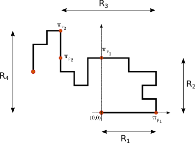
Figure 2: We decompose a path $\pi\in\Omega_{L}$ into a sequence of excursions. The $i$-th excursion is a horizontal excursion if $i$ is odd, and vertical excursion if $i$ is even. The $1$-st excursion corresponds to the sub-path $\pi_{[0,\rho_{1}]}$, the $2$-nd to the sub-path $\pi_{[\rho_{1},\upsilon 1]}$ and so on. At the end of the $i$-th excursion, if $i$ is odd (resp. if $i$ is even) we set $R_{i}$ to be the width (resp. the height) of the range. The last excursion is incomplete.

4.2 Effective random walk excursion in a slab

The one-to-one correspondence in Section 3.2 between the excursion paths (which are partially directed) and the effective random walk paths can be extended to the current setting, except that now the effective random walk lies in a slab corresponding to the range of the path at the start of the excursion, and the excursion may end on either side of the slab. As a consequence, we define a measure $L_{R}$ on $\mathbb{N}\times\mathbb{N}\times\{0,1\}$ by

$$L_{R}(t,n,0) =\boldsymbol{\mathrm{E}}\Big{[}e^{\log(\frac{3}{2})n-\lambda^{*}t}\,{\sf 1}_{\{V_{i}\in\{0,\dots,R\}\ \forall i\leq n,\,V_{n}=0,\,\sum_{i=1}^{n}|U_{i}|=t-n\}}\Big{]},$$ (4.3)

$$L_{R}(t,n,1) =\boldsymbol{\mathrm{E}}\Big{[}e^{\log(\frac{3}{2})n-\lambda^{*}t}\,{\sf 1}_{\{V_{i}\in\{0,\dots,R\}\ \forall i\leq n,\,V_{n}=R,\,\sum_{i=1}^{n}|U_{i}|=t-n\}}\Big{]}.$$

When $R=0$, define $L_{0}(t,n,1)$ as above and define $L_{0}(t,n,0)=0$. Let $\widehat{L}_{R}$ be a variant of $L_{R}$ that accounts for an incomplete excursion (cf. Figure 2), i.e.,

$$\widehat{L}_{R}(t,n) =\boldsymbol{\mathrm{E}}\Big{[}e^{\log(\frac{3}{2})n-\lambda^{*}t}\,{\sf 1}_{\{V_{i}\in\{0,\dots,R\}\ \forall i\leq n,\,0<V_{n}<R,\,\sum_{i=1}^{n}|U_{i}|=t-n\}}\Big{]},$$ (4.4)

where $\lambda^{*}$ is as in Lemma 3.4. We also set $\widehat{L}_{R}(t)=\sum_{n\geq 1}\widehat{L}_{R}(t,n)$ and $\widehat{L}_{R}(0)=1$.

Let $\alpha^{*}=\log(\frac{3}{2})-\lambda^{*}$, and let $(t_{i},n_{i},\varepsilon_{i})\in\mathbb{N}^{2}\times\{0,1\}$, $1\leq i\leq r$, be such that $t_{1}+\dots+t_{r}\leq L$ and $n_{i}\leq t_{i}$. Let $\Omega_{L}\big{(}(t_{i},n_{i},\varepsilon_{i})_{i=1}^{r}\big{)}$ be the set of prudent paths containing $r$ complete excursions, with $(T_{i},N_{i},{\mathcal{E}}_{i})_{i=1}^{r}=(t_{i},n_{i},\varepsilon_{i})_{i=1}^{r}$, and recall $(R_{i-1})_{i\in\mathbb{N}}$ from the end of Section 4.1. Reasoning as for (3.14), we then have

$$\frac{1}{2^{L}}|\Omega_{L}\big{(}(t_{i},n_{i},\varepsilon_{i})_{i=1}^{r}\big{)}|e^{-\lambda^{*}L}= \prod_{i=1}^{r}\boldsymbol{\mathrm{E}}\bigg{[}e^{\alpha^{*}n_{i}-\lambda^{*}(t_{i}-n_{i})}\,{\sf 1}_{\big{\{}V_{i}\in[0,R_{i-1}]\,\forall i\leq n_{i},\,V_{n_{i}}=\varepsilon_{i}R_{i-1},\,n_{i}+\sum_{j=1}^{n_{i}}|U_{j}|=t_{i}\big{\}}}\bigg{]}$$

$$\quad\times\,\widehat{L}_{R_{r}}\big{(}L-(t_{1}+\dots+t_{r})\big{)}$$ (4.5)

$$= \bigg{[}\prod_{i=1}^{r}L_{R_{i-1}}(t_{i},n_{i},\varepsilon_{i})\bigg{]}\,\widehat{L}_{R_{r}}\big{(}L-(t_{1}+\dots+t_{r})\big{)},$$

where $\widehat{L}_{R_{r}}(L-(t_{1}+\dots+t_{r}))$ accounts for the last incomplete excursion in $\pi$.

4.3 Representation of the law of a uniform prudent walk

We now show how to represent the law of the uniform prudent walk in terms of the excursions of the effective random walk $V$.

For $R\in\mathbb{N}$, let ${\mathcal{V}}_{R}$ be the set of effective random walk paths in a slab of width $R$ and ending at either $0$ or $R$. Namely,

$${\mathcal{V}}_{R}:=\bigcup_{N\geq 1}\Big{[}{\mathcal{V}}^{\,1}_{N,R}\cup{\mathcal{V}}^{\,0}_{N,R}\Big{]},$$ (4.6)

where for $a=0,1$,

$${\mathcal{V}}_{N,R}^{\,a}:=\Big{\{}(V_{i})_{i=0}^{N}\colon\,V_{0}=0,V_{i}\in\{0,\dots,R\}\ \forall i\in\{0,\dots,N\},V_{N}=aR\Big{\}}.$$ (4.7)

Recall the effective random walk excursion measure $\boldsymbol{\mathrm{P}}^{*}$ from (3.13). We will define a probability law $\boldsymbol{\mathrm{P}}_{R}^{*}$ on ${\mathcal{V}}_{R}$ by sampling a path under $\boldsymbol{\mathrm{P}}^{*}$ and truncating it if it passes above $R+1$. More precisely, define the truncation $T_{R}:{\mathcal{V}}_{\infty}\mapsto{\mathcal{V}}_{R}$ as follows. Given $V:=(V_{i})_{i=0}^{N}\in{\mathcal{V}}_{\infty}$, let $T_{R}V:=V$ if $V_{i}\leq R$ for every $i\leq N$. Otherwise, let $\tau_{R}:=\inf\{i\geq 1\colon V_{i}\geq R+1\}$ and set

$$(T_{R}V)_{i}=V_{i}\quad\text{for $i\leq\tau_{R}-1$ and}\ (T_{R}V)_{\tau_{R}}=R.$$ (4.8)

Then define $\boldsymbol{\mathrm{P}}_{R}^{*}$ as the image measure of $\boldsymbol{\mathrm{P}}^{*}$ under $T_{R}$. For each trajectory $V\in{\mathcal{V}}_{R}$, we associate $(T,N,{\mathcal{E}})$ such that $N$ is the number of increments $(U_{i})_{i=1}^{N}$ of $V$, $T=N+\sum_{i=1}^{N}|U_{i}|$, and ${\mathcal{E}}=1$ if $V_{N}=R$ and ${\mathcal{E}}=0$ if $V_{N}=0$ (if $R=0$, set ${\mathcal{E}}=1$). Let $L^{*}_{R}$ denote the law of $(T,N,{\mathcal{E}})$ when $V$ is sampled from $\boldsymbol{\mathrm{P}}_{R}^{*}$, and we observe that $L_{R}^{*}$ and $L_{R}$ (cf. (4.3)) coincide when $\varepsilon=0$, i.e.,

$$L_{R}(t,n,0)=L_{R}^{*}(t,n,0),\quad(t,n)\in\mathbb{N}\times\mathbb{N}.$$ (4.9)

Let $(\widetilde{V}^{(i)})_{i\geq 1}$ be an i.i.d. sequence of effective walk excursions with law $\boldsymbol{\mathrm{P}}^{*}$, and for each $i\in\mathbb{N}$, let $(\widetilde{T}_{i},\widetilde{N}_{i})$ denote the total length and the number of increments of $\widetilde{V}^{(i)}$. We now construct a sequence $(T_{i},N_{i},{\mathcal{E}}_{i})_{i\geq 1}$ from $(\widetilde{V}^{(i)})_{i\geq 1}$ inductively, using the truncation map $T_{R}$. First set $R_{-1}=R_{0}:=0$. For each $i\geq 1$, set

$$V^{(i)}=T_{R_{i-1}}\widetilde{V}^{(i)},\qquad(N_{i},T_{i},{\mathcal{E}}_{i})=(N,T,{\mathcal{E}})(V^{(i)}),\quad\text{and}\quad R_{i}=R_{i-2}+N_{i}.$$ (4.10)

where $(N,T,{\mathcal{E}})(V^{(i)})$ is the triple $(N,T,{\mathcal{E}})$ associated with $V^{(i)}\in{\mathcal{V}}_{R_{i-1}}$. For every $i\geq 1$, we have $N_{i}\leq\widetilde{N}_{i}$ and $T_{i}\leq\widetilde{T}_{i}$, and conditioned on $(T_{j},N_{j},{\mathcal{E}}_{j})_{j=1}^{i-1}$, the law of $(N_{i},T_{i},{\mathcal{E}}_{i})$ is $\boldsymbol{\mathrm{P}}_{R_{i-1}}^{*}$. Note that the excursion decomposition of a prudent path in Section 4.1 gives exactly a sequence of excursions of the form $(T_{R}\widetilde{V}^{(i)})_{i\geq 1}$.

For a set of prudent paths $A\subset\Omega_{L}$ depending only on $(T_{i},N_{i},{\mathcal{E}}_{i})_{i=1}^{\gamma_{L}}(\pi)$, where

$$\gamma_{L}=\min\{i\geq 1\colon\,T_{1}+\dots+T_{i}>L\}-1,$$ (4.11)

let $(t_{i},n_{i},\varepsilon_{i})_{i=1}^{r}\sim A$ denote compatibility with $A$. By (4.5), we then have

$$\frac{1}{2^{L}}|A|e^{-\lambda^{*}L}=\sum_{(t_{i},n_{i},\varepsilon_{i})_{i=1}^{r}\sim A}\bigg{[}\prod_{i=1}^{r}L_{R_{i-1}}(t_{i},n_{i},\varepsilon_{i})\bigg{]}\,\widehat{L}_{R_{r}}\big{(}L-(t_{1}+\dots+t_{r})\big{)}$$

$$=\ \boldsymbol{\mathrm{E}}^{*}\Bigg{[}{\sf 1}_{\{(T_{i},N_{i},{\mathcal{E}}_{i})_{i=1}^{\gamma_{L}}\sim A\}}\prod_{i=1}^{\gamma_{L}}\ \frac{L_{R_{i-1}}(T_{i},N_{i},{\mathcal{E}}_{i})}{L^{*}_{R_{i-1}}(T_{i},N_{i},{\mathcal{E}}_{i})}\,\cdot\,\frac{\widehat{L}_{R_{\gamma_{L}}}(L-(T_{1}+\dots+T_{\gamma_{L}}))}{\boldsymbol{\mathrm{P}}_{R_{\gamma_{L}}}^{*}\big{(}T>L-(T_{1}+\dots+T_{\gamma_{L}}\big{)}}\Bigg{]},$$ (4.12)

where $\boldsymbol{\mathrm{E}}^{*}$ is expectation over the i.i.d. excursions $(\widetilde{V}^{(i)})_{i\geq 1}$, and hence $(T_{i},N_{i},{\mathcal{E}}_{i})_{i\geq 1}$.

We conclude this section with two technical lemmas needed to control the ratios inside the expectation in (4.3). For ease of notation, let us denote

$$L_{R}(t,\varepsilon):=\sum_{n\geq 1}L_{R}(t,n,\varepsilon)\qquad\mbox{and}\qquad L_{R}(t):=L_{R}(t,0)+L_{R}(t,1).$$ (4.13)

Lemma 4.1.

There exists $C>0$ such that

$$\frac{L_{R}(t)}{L_{R}^{*}(t)}\leq C\,t\,{\sf 1}_{\{t\geq R\}}\,+\,{\sf 1}_{\{t<R\}}\qquad\mbox{for all }t\in\mathbb{N}.$$ (4.14)

Proof.

First, observe that for $t<R$, a path of length $t$ cannot reach level $R$. Therefore, $L_{R}(t,n,1)=L^{*}_{R}(t,n,1)=0$ and $L_{R}(t,n,1)=L^{*}_{R}(t,n,1)$. It only remains to consider $t\geq R$, and it suffices to show that $L_{R}(t,1)\leq CtL_{R}(t,0)=CtL_{R}^{*}(t)$. For simplicity we only consider the case $R\in 2\mathbb{N}$, but the case $R\in 2\mathbb{N}+1$ can be treated in a similar manner. Let

$${\mathcal{B}}_{n,t}^{R}:= \Big{\{}(V_{i})_{i=0}^{n}\colon\,V_{0}=0,V_{i}\in\{0,\dots,R\}\ \forall i\in\{0,\dots,n\},V_{n}=R,\sum_{i=1}^{n}|U_{i}|=t-n\Big{\}},$$ (4.15)

$${\mathcal{A}}_{n,t}^{R}:= \Big{\{}(V_{i})_{i=0}^{n}\colon\,V_{0}=0,V_{i}\in\{0,\dots,R\}\ \forall i\in\{0,\dots,n\},V_{n}=0,\sum_{i=1}^{n}|U_{i}|=t-n\Big{\}}.$$ (4.16)

We define a map $G_{n,t}^{R}:{\mathcal{B}}_{n,t}^{R}\mapsto{\mathcal{A}}_{n,t}^{R}\cup{\mathcal{A}}_{n+2,t}^{R}$ as follows. For $V\in{\mathcal{B}}_{n,t}^{R}$, let $\tau_{R/2}:=\min\{i\geq 1\colon\,V_{i}\geq R/2\}$. We distinguish between two cases (see Figure 3):

1. If $V_{\tau_{R/2}}=R/2$, then define $G_{n,t}^{R}(V)$ by simply reflecting $V$ across $R/2$ from $\tau_{R/2}$ onward, i.e., $G_{n,t}^{R}(V)_{i}=V_{i}$ for $i\leq\tau_{R/2}$ and $G_{n,t}^{R}(V)_{i}=R-V_{i}$ for $i\in\{\tau_{R/2},\dots,n\}$. Then, $G_{n,t}^{R}(V)\in{\mathcal{A}}_{n,t}^{R}$.
   

2. If $V_{\tau_{R/2}}=R/2+y$ with $y\in\{1,\dots,\frac{R}{2}\}$, then let $G_{n,t}^{R}(V)_{i}=V_{i}$ for $i\leq\tau_{R/2}-1$, $G_{n,t}^{R}(V)_{\tau_{R/2}}=\frac{R}{2}-1$, $G_{n,t}^{R}(V)_{i}=R-V_{i-1}$ for $i\in\{\tau_{R/2}+1,\dots,n+1\}$ and $G_{n,t}^{R}(V)_{n+2}:=0$. Then, $G_{n,t}^{R}(V)\in{\mathcal{A}}_{n+2,t}^{R}$.

Note that under $G_{n,t}^{R}$, every $V\in G_{n,t}^{R}({\mathcal{B}}_{n,t}^{R})\cap{\mathcal{A}}_{n,t}^{R}$ has a unique pre-image in ${\mathcal{B}}_{n,t}^{R}$, and every $V\in G_{n,t}^{R}({\mathcal{B}}_{n,t}^{R})\cap{\mathcal{A}}_{n+2,t}^{R}$ has at most $n\leq t$ pre-images in ${\mathcal{B}}_{n,t}^{R}$, one for each time that $V$ is at level $\frac{R}{2}-1$. Finally, we note that in the second case, $G_{n,t}^{R}(V)$ has two fewer vertical steps and two more horizontal steps than $V$. This allows us to write

$$L_{R}(t,1) =\sum_{n=1}^{t}\boldsymbol{\mathrm{E}}\Big{[}e^{\log(\frac{3}{2})n-\lambda^{*}t}\ {\sf 1}_{{\mathcal{B}}_{n,t}^{R}}(V)\Big{]}$$ (4.17)

$$\leq\sum_{n=1}^{t}\boldsymbol{\mathrm{E}}\Big{[}e^{\log(\frac{3}{2})n-\lambda^{*}t}\ {\sf 1}_{{\mathcal{A}}_{n,t}^{R}}(V)\Big{]}+t\,\boldsymbol{\mathrm{E}}\Big{[}e^{\log(\frac{3}{2})(n+2)-\lambda^{*}t}\ {\sf 1}_{{\mathcal{A}}_{n+2,t}^{R}}(V)\Big{]}.$$

Observe that the r.h.s. in (4.17) is less than $\sum_{n=1}^{t}L_{R}(n,t,0)+tL_{R}(n+2,t,0)$, which implies

$$L_{R}(t,1) \leq 2tL_{R}(t,0).$$ (4.18)

This concludes the proof of the lemma. ∎

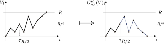
(a)

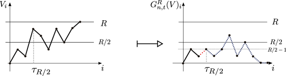
(b)

Figure 3: The transformation $G_{n,t}^{R}(V)$. We let $\tau_{R/2}:=\min\{i\geq 1\colon V_{i}\geq R/2\}$. In $(\textrm{a})$ we draw the case in which $V_{\tau_{R/2}}=R/2$. In this case we define $G_{n,t}^{R}(V)$ by simply reflecting $V$ across $R/2$ from $\tau_{\tau_{R/2}}$ onward (in blue, dotted). In $(\textrm{b})$ we draw the case in which $V_{\tau_{R/2}}>R/2$. In this second case we let $G_{n,t}^{R}(V)_{\tau_{R/2}}=\frac{R}{2}-1$ (in red, dotted) and we concatenate the reflection of $V$ across $R/2$ from $\tau_{R/2}$ onward. We add a final point $G_{n,t}^{R}(V)_{n+2}:=0$ (in blue, dotted).

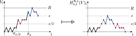
Figure 4: The transformation $H_{n,t}^{R,x}(V)$: We fix $x\leq R$ even and we consider a path $V$ ending at $V_{n}=x$. We let $\sigma_{x/2}:=\max\{i\geq 0\colon\,V_{i}<\tfrac{x}{2}\}$ and $\widetilde{\sigma}_{x}:=\min\{i\geq\sigma_{x/2}+1\colon\,V_{i}\geq x\}.$ In the figure we draw the transformation $H_{n,t}^{R,x}(V)$ when $V_{\sigma_{x/2}+1}>x/2$ and $V_{\widetilde{\sigma}_{x}}>x$. In this case we define $H_{n,t}^{R,x}(V)_{\sigma_{x/2}+1}:=x/2$. Then we take the piece of $V$ on the interval $[\widetilde{\sigma}_{x},n]$ lowered by $x/2$ and we insert it at time $\sigma_{x/2}+2$ (blue). Finally the piece of $V$ on the interval $[\sigma_{x/2}+1,\widetilde{\sigma}_{x}-1]$ is reflected across $x/2$ and reattached at the end (violet). We add a final point $H_{n,t}^{R,x}(V)_{n+2}:=0$.

To bound the last ratio in (4.3), we will bound $\widehat{L}_{R}(t)/\boldsymbol{\mathrm{P}}_{R}^{*}\big{(}T\geq t\big{)}$, which arises from the last incomplete excursion in the excursion decomposition. Recall that $\widehat{L}_{R}(0):=1=\boldsymbol{\mathrm{P}}_{R}^{*}(T>0)$.

Lemma 4.2.

There exists $C>0$ such that

$$\frac{\widehat{L}_{R}(t)}{\boldsymbol{\mathrm{P}}_{R}^{*}(T>t)}\leq CRt^{2}\quad\mbox{ for all }R,t\in\mathbb{N}.$$ (4.19)

Proof.

Recall $\widehat{L}_{R}(t)$ from (4.4). It suffices to show that there exists $C>0$ such that

$$\widehat{L}_{R}(t)\leq CR\,t^{2}L_{R}(t+2,0),$$ (4.20)

since

$$\boldsymbol{\mathrm{P}}_{R}^{*}\big{(}T>t\big{)}=\sum_{j>t}L^{*}_{R}(j)\geq\sum_{j>t}L_{R}^{*}(j,0)=\sum_{j>t}L_{R}(j,0)\geq L_{R}(t+2,0).$$

For $x\in\{1,\dots,R-1\}$ and $n\leq t$, we consider the set of effective random walk trajectories

$${\mathcal{D}}_{n,t}^{R,x}= \Big{\{}(V_{i})_{i=0}^{n}\colon\,V_{0}=0,V_{i}\in\{0,\dots,R\}\ \forall i\in\{0,\dots,n\},V_{n}=x,\sum_{i=1}^{n}|U_{i}|=t-n\Big{\}}.$$ (4.21)

For simplicity, we assume that $x$ is even, but the case $x$ odd can be treated similarly. Let

$$\sigma_{x/2}:=\max\{i\geq 0\colon\,V_{i}<\tfrac{x}{2}\}\quad\text{and}\quad\widetilde{\sigma}_{x}:=\min\{i\geq\sigma_{x/2}+1\colon\,V_{i}\geq x\}.$$ (4.22)

We define a map $H_{n,t}^{R,x}:{\mathcal{D}}_{n,t}^{R,x}\to{\mathcal{A}}_{n+2,t+2}^{R}$ (cf. (4.16)) as follows. Let $V\in{\mathcal{D}}_{n,t}^{R,x}$. We distinguish between four cases:

1. $V_{\sigma_{x/2}+1}>x/2$ and $V_{\widetilde{\sigma}_{x}}>x$,

2. $V_{\sigma_{x/2}+1}>x/2$ and $V_{\widetilde{\sigma}_{x}}=x$,

3. $V_{\sigma_{x/2}+1}=x/2$ and $V_{\widetilde{\sigma}_{x}}>x$,

4. $V_{\sigma_{x/2}+1}=x/2$ and $V_{\widetilde{\sigma}_{x}}=x$.

We will treat case 1 only, where $H_{n,t}^{R,x}$ maps $V$ to a path in ${\mathcal{A}}_{n+2,t+2}^{R}$ (see Figure 4). Cases 2–4 are similar and even simpler, and to ensure that $H_{n,t}^{R,x}(V)\in{\mathcal{A}}_{n+2,t+2}^{R}$, we can add extra horizontal steps if needed. Roughly speaking, under $H_{n,t}^{R,x}$, the piece of $V$ on the interval $[\widetilde{\sigma}_{x},n]$ is lowered by $x/2$ and inserted at time $\sigma_{x/2}+2$, while the piece of $V$ on the interval $[\sigma_{x/2}+1,\widetilde{\sigma}_{x}-1]$ is reflected across $x/2$ and reattached at the end. More precisely, set

$$H_{n,t}^{R,x}(V)_{i}:=V_{i}\quad\text{for}\quad i\leq\sigma_{x/2},$$

$$H_{n,t}^{R,x}(V)_{\sigma_{x/2}+1}:=x/2,$$

$$H_{n,t}^{R,x}(V)_{\sigma_{x/2}+1+i}:=V_{\widetilde{\sigma}_{x}+i-1}-x/2\quad\text{for}\quad i=1,\dots,n+1-\widetilde{\sigma}_{x},$$

$$H_{n,t}^{R,x}(V)_{n+2-(\widetilde{\sigma}_{x}-\sigma_{x/2})+i}:=x-V_{\sigma_{x/2}+i}\quad\text{for}\quad i=1,\dots,\widetilde{\sigma}_{x}-\sigma_{x/2}-1,$$

$$H_{n,t}^{R,x}(V)_{n+2}:=0.$$

We note that the sum of absolute increments of $H_{n,t}^{R,x}(V)$ equals that of $V$, and $H_{n,t}^{R,x}(V)$ is confined to $[0,R]$. Therefore $H_{n,t}^{R,x}(V)\in{\mathcal{A}}_{n+2,t+2}^{R}$. It remains to bound the number of pre-images of every $V\in{\mathcal{A}}_{n+2,t+2}^{R}\cap H_{n,t}^{R,x}({\mathcal{D}}_{n,t}^{R,x})$ under $H_{n,t}^{R,x}$. Note that to undo $H_{n,t}^{R,x}(V)$, we only need to find the two times $\sigma_{x/2}+2$ and $\sigma_{x/2}+n+2-\widetilde{\sigma}_{x}$ at which the original segments of $V$ are glued together and $H_{n,t}^{R,x}(V)_{i}=0$. Since there are at most $n^{2}\leq t^{2}$ such choices, and combined with similar estimates for cases 2–4, we have

$$\widehat{L}_{R}(t,n) =\sum_{x=1}^{R-1}\boldsymbol{\mathrm{E}}\Big{[}e^{\log(\frac{3}{2})n-\lambda^{*}t}\,{\sf 1}_{\,{\mathcal{D}}_{n,t}^{R,x}}(V)\Big{]}$$ (4.23)

$$\leq 4(R-1)\,t^{2}\Big{(}3^{2}e^{-2\log(\frac{3}{2})+2\lambda^{*}}\boldsymbol{\mathrm{E}}\Big{[}e^{\log(\frac{3}{2})(n+2)-\lambda^{*}(t+2)}\,{\sf 1}_{\,{\mathcal{A}}_{n+2,t+2}^{R}}(V)\Big{]}\Big{)}$$

$$\leq CR\,t^{2}L_{R}(t+2,n+2,0),$$

which establishes (4.20) and hence the lemma. ∎

As a corollary of Lemma 4.2, we have the following bound on the last ratio in (4.3):

$$\frac{\widehat{L}_{R_{\gamma_{L}}}(L-(T_{1}+\cdots+T_{\gamma_{L}}))}{\boldsymbol{\mathrm{P}}_{R_{\gamma_{L}}}^{*}\big{(}T>L-(T_{1}+\cdots+T_{\gamma_{L}})\big{)}}\leq C\,L(L-(T_{1}+\cdots+T_{\gamma_{L}}))^{2}.$$ (4.24)

5 Proof of Theorems 2.2 and 2.3

We will use the excursion decomposition developed in Section 4, in particular, the representation in (4.3). First we show that for large $L$, a uniform prudent walk typically crosses its range at most $\log L$ times. Namely,

Lemma 5.1.

There exists $\delta>0$ such that

$$\lim_{L\to\infty}\boldsymbol{\mathrm{P}}_{{\rm unif},L}\big{[}\exists\,i\in\{\delta\log L,\dots,\gamma_{L}(\pi)\}\colon\,{\mathcal{E}}_{i}(\pi)=1\big{]}=0.$$ (5.1)

Then we show that the total length of the first $\log L$ excursions grows less than a power of $\log L$.

Lemma 5.2.

For every $\delta>0$, there exists $\kappa>0$ such that

$$\lim_{L\to\infty}\boldsymbol{\mathrm{P}}_{{\rm unif},L}\big{[}T_{1}(\pi)+\dots+T_{\delta\log L}(\pi)\geq\kappa\,(\log L)^{2}\big{]}=0.$$ (5.2)

Finally, we show that the last incomplete excursion of the walk typically has length at most $\log L$.

Lemma 5.3.

There exists $\alpha>0$ such that

$$\lim_{L\to\infty}\boldsymbol{\mathrm{P}}_{{\rm unif},L}\big{[}L-(T_{1}+\dots+T_{\gamma_{L}})\geq\alpha\log L\big{]}=0.$$ (5.3)

We prove Theorem 2.2 next using Lemmas 5.1–5.3, whose proof are postponed to Sections 5.2–5.4.

5.1 Proof of Theorems 2.2 and 2.3

Let $\delta,\kappa,\alpha>0$, and we define ${\mathcal{G}}_{L}\subset\Omega_{L}$ by

$${\mathcal{G}}_{L}:=\Big{\{}{\mathcal{E}}_{i}=0\,\forall\,i\in\{\delta\log L,\dots,\gamma_{L}\},\,T_{1}+\dots+T_{\delta\log L}\leq\kappa(\log L)^{2},\ L-(T_{1}+\dots+T_{\gamma_{L}})\leq\alpha\log L\Big{\}}.$$

By Lemmas 5.1–5.3, we can choose $\delta,\kappa$ and $\alpha$ such that $\lim_{L\to\infty}\boldsymbol{\mathrm{P}}_{\text{unif},L}\big{(}{\mathcal{G}}_{L}\big{)}=1$.

We introduce a little more notation. Let ${\mathcal{O}}:=\{\text{NE,NW,SE,SW}\}$ be the set of possible directions of a 2-sided prudent path. For $o\in{\mathcal{O}}$ let $\Omega_{L}^{\,o}$ be the set of $L$-step 2-sided path with orientation $o$ (e.g. $\Omega_{L}^{\text{NE}}=\Omega_{L}^{+}$). Pick $\pi\in\Omega_{L}$ and recall that the endpoint of each excursion of $\pi$ lies at one of the 4 corners (indexed in ${\mathcal{O}}$) of the smallest rectangle containing the range of $\pi$ up to that endpoint. Thus, for $\pi\in{\mathcal{G}}_{L}$, we denote by $\vartheta(\pi)\in{\mathcal{O}}$ the corner at which the endpoint of the $\delta\log L$-th excursion lies.

For a path $\pi\in{\mathcal{G}}_{L}$, let $\sigma_{1}:=T_{1}+\dots+T_{\delta\log L}$ be the length of the first $\delta\log L$ excursions, and let $\sigma_{2}:=L-(T_{1}+\dots+T_{\gamma_{L}})$ be the length of the last incomplete excursion. Note that $(\pi_{i})_{i=\sigma_{1}}^{L-\sigma_{2}}$ is a 2-sided prudent path of orientation $\vartheta(\pi)$ because ${\mathcal{E}}_{i}=0$ for $\delta\log L<i\leq\gamma_{L}(\pi)$. Therefore, we can safely enlarge a bit ${\mathcal{G}}_{L}$ into

$$\widetilde{\mathcal{G}}_{L}:=\Big{\{}(\pi_{i})_{i=\sigma_{1}}^{L-\sigma_{2}}\in\Omega_{L-\sigma_{1}-\sigma_{2}}^{\vartheta(\pi)},\,T_{1}+\dots+T_{\delta\log L}\leq\kappa(\log L)^{2},\ L-(T_{1}+\dots+T_{\gamma_{L}})\leq\alpha\log L\Big{\}}.$$

Note that conditioned on $\pi\in\widetilde{\mathcal{G}}_{L}$, $\sigma_{1}(\pi)=m$, $\sigma_{2}(\pi)=n$, and $\vartheta(\pi)=o$, the law of $(\pi_{i})_{i=m}^{L-n}$ under $\boldsymbol{\mathrm{P}}_{\text{unif},L}$ (modulo translation and rotation) is exactly that of a uniform 2-sided prudent walk with total length $L-m-n$, for which we have proved the law of large numbers in Theorem 3.1 and the invariance principle in Theorem 3.2. Since $\boldsymbol{\mathrm{P}}_{\text{unif},L}\big{(}\widetilde{\mathcal{G}}_{L}\big{)}\to 1$, we only need to consider $m\leq\kappa(\log L)^{2}$ and $n\leq\alpha\log L$. Since $m/\sqrt{L},n/\sqrt{L}$ tend to $0$ uniformly as $L$ tends to infinity, $(\pi_{i})_{i=1}^{m}$ and $(\pi_{i})_{i=L-n}^{L}$ are negligible in the scaling limit, and hence Theorems 2.2 and 2.3 follow from their counterparts for the uniform 2-sided prudent walk, with the direction $o$ distributed uniformly in ${\mathcal{O}}$ by symmetry. ∎

5.2 Proof of Lemma 5.1

Let $M=M(L)$ be an increasing function of $L$ that will be specified later. We set

$$\alpha_{L}:=\boldsymbol{\mathrm{P}}_{\text{unif},L}\big{(}\exists\,i\in[M,\gamma_{L}]\,s.t.\,{\mathcal{E}}_{i}(\pi)=1\big{)}=\frac{\big{|}\{\pi\in\Omega_{L}:\,\exists\,i\in[M,\gamma_{L}]\,s.t.\,{\mathcal{E}}_{i}(\pi)=1\}\big{|}}{|\Omega_{L}|}.$$ (5.4)

Multiply both the numerator and denominator by $2^{-L}e^{-\lambda^{*}L}$, we can then apply (4.3) together with (4.24) to obtain

$$\alpha_{L} \leq CL^{3}\frac{\,\sum_{j=M}^{L}\boldsymbol{\mathrm{E}}^{*}\Big{[}{\sf 1}_{\{{\mathcal{E}}_{j}=1\}}\,\prod_{i=1}^{\gamma_{L}}\frac{L_{R_{i-1}}(T_{i},N_{i},{\mathcal{E}}_{i})}{L^{*}_{R_{i-1}}(T_{i},N_{i},{\mathcal{E}}_{i})}\Big{]}}{\boldsymbol{\mathrm{E}}^{*}\Big{[}\prod_{i=1}^{\gamma_{L}}\frac{L_{R_{i-1}}(T_{i},N_{i},{\mathcal{E}}_{i})}{L^{*}_{R_{i-1}}(T_{i},N_{i},{\mathcal{E}}_{i})}{\sf 1}_{\{T_{1}+\dots+T_{\gamma_{L}}=L\}}\Big{]}}$$

$$\leq CL^{3}\frac{\,\sum_{j\geq M}\boldsymbol{\mathrm{E}}^{*}\Big{[}{\sf 1}_{\{T_{j}\geq\frac{j}{2}\}}\,\prod_{i=1}^{\gamma_{L}}\frac{L_{R_{i-1}}(T_{i},N_{i},{\mathcal{E}}_{i})}{L^{*}_{R_{i-1}}(T_{i},N_{i},{\mathcal{E}}_{i})}\Big{]}}{\boldsymbol{\mathrm{E}}^{*}\Big{[}\prod_{i=1}^{\gamma_{L}}\frac{L_{R_{i-1}}(T_{i},N_{i},{\mathcal{E}}_{i})}{L^{*}_{R_{i-1}}(T_{i},N_{i},{\mathcal{E}}_{i})}{\sf 1}_{\{T_{1}+\dots+T_{\gamma_{L}}=L\}}\Big{]}}:=CL^{3}\frac{\Psi_{1}(L,M)}{D_{L}},$$ (5.5)

where we used that ${\mathcal{E}}_{i}=1$ only if $T_{i}\geq 1+R_{i-1}$, and $R_{i}\geq\frac{i-1}{2}$ for every $i\in\mathbb{N}$ (cf. Section 4.1). Lemma 5.1 then follows immediately from (5.5) and Claims 5.4 and 5.5 below.

Claim 5.4.

There exist $c_{1},c_{2}>0$ such that $\Psi_{1}(L,M)\leq c_{1}\,e^{-c_{2}M}$ for every $M\in\mathbb{N}$ and $L\geq M$.

Claim 5.5.

There exists $c_{3}>0$ such that $D_{L}\geq c_{3}$ for every $L\in\mathbb{N}$.

Proof of Claim 5.4. Recall from Section 4.3 how $(T_{i},N_{i},{\mathcal{E}}_{i})_{i\geq 1}$ is constructed from the i.i.d. sequence $(\widetilde{V}_{i},\widetilde{T}_{i},\widetilde{N}_{i})_{i\geq 1}$ with law $\boldsymbol{\mathrm{P}}^{*}$, with $\widetilde{T}_{i}\geq T_{i}\,\forall\,i\in\mathbb{N}$. We first state and prove a key lemma.

Lemma 5.6.

Let $L\in\mathbb{N}$, and let $\Phi:\mathbb{R}^{L}_{+}\to\mathbb{R}_{+}$ be any function that is non-decreasing in each of its $L$ arguments. Then there exists $c>0$ independent of $L$ and $\Phi$, such that

$$\boldsymbol{\mathrm{E}}^{*}\bigg{[}\!\Phi(T_{1},\dots,T_{L})\prod_{i=1}^{\gamma_{L}}\frac{L_{R_{i-1}}(T_{i},N_{i},{\mathcal{E}}_{i})}{L^{*}_{R_{i-1}}(T_{i},N_{i},{\mathcal{E}}_{i})}\bigg{]}\leq\boldsymbol{\mathrm{E}}^{*}\bigg{[}\Phi(\widetilde{T}_{1},\dots,\widetilde{T}_{L})\prod_{i=1}^{L}\big{(}1+c\widetilde{T}_{i}\,{\sf 1}_{\{\widetilde{T}_{i}\geq\frac{i-1}{2}\}}\big{)}\bigg{]}.$$ (5.6)

Proof.

For $n\in\mathbb{N}$, let ${\mathcal{F}}_{n}$ be the $\sigma$-algebra generated by $(\widetilde{T}_{i},T_{i},N_{i},{\mathcal{E}}_{i})_{i\leq n}$. For ease of notation, let $A_{L}$ denote the l.h.s. of (5.6). Note that

$$A_{L} \leq\boldsymbol{\mathrm{E}}^{*}\bigg{[}\Phi(T_{1},\dots,T_{L})\prod_{i=1}^{L}\max\bigg{\{}\frac{L_{R_{i-1}}(T_{i},N_{i},{\mathcal{E}}_{i})}{L^{*}_{R_{i-1}}(T_{i},N_{i},{\mathcal{E}}_{i})},1\bigg{\}}\bigg{]}$$ (5.7)

$$=\boldsymbol{\mathrm{E}}^{*}\bigg{[}\prod_{i=1}^{L-1}\max\Big{\{}\frac{L_{R_{i-1}}(T_{i},N_{i},{\mathcal{E}}_{i})}{L^{*}_{R_{i-1}}(T_{i},N_{i},{\mathcal{E}}_{i})},1\Big{\}}\,\,H_{L}\bigg{]},$$ (5.8)

with

$$\begin{split}H_{L}&:=\boldsymbol{\mathrm{E}}^{*}\bigg{[}\Phi(T_{1},\dots,T_{L})\max\Big{\{}\frac{L_{R_{L-1}}(T_{L},N_{L},{\mathcal{E}}_{L})}{L^{*}_{R_{L-1}}(T_{L},N_{L},{\mathcal{E}}_{L})},1\Big{\}}\Big{|}{\mathcal{F}}_{L-1}\bigg{]}\\ &\ =\sum_{t}\Phi(T_{1},\dots,T_{L-1},t)\sum_{n\leq t}\sum_{\varepsilon=0,1}\max\big{\{}{L_{R_{L-1}}(t,n,\varepsilon)},L^{*}_{R_{L-1}}(t,n,\varepsilon)\big{\}}.\end{split}$$ (5.9)

When $t<R_{L-1}$, we have ${L_{R_{L-1}}(t,n,1)}=L^{*}_{R_{L-1}}(t,n,1)=0$, and ${L_{R_{L-1}}(t,n,0)}=L^{*}_{R_{L-1}}(t,n,0)$ by (4.9), so that

$$\sum_{n\leq t}\sum_{\varepsilon=0,1}\max\big{\{}{L_{R_{L-1}}(t,n,\varepsilon)},L^{*}_{R_{L-1}}(t,n,\varepsilon)\big{\}}=L^{*}_{R_{L-1}}(t).$$ (5.10)

When $t\geq R_{L-1}$, we have

$$\begin{split}&\sum_{n\leq t}\sum_{\varepsilon=0,1}\max\big{\{}{L_{R_{L-1}}(t,n,\varepsilon)},L^{*}_{R_{L-1}}(t,n,\varepsilon)\big{\}}\\ &\quad\leq\ \sum_{n\leq t}\sum_{\varepsilon=0,1}({L_{R_{L-1}}(t,n,\varepsilon)}+L^{*}_{R_{L-1}}(t,n,\varepsilon))=L_{R_{L-1}}(t)+L^{*}_{R_{L-1}}(t)\leq(1+ct)L^{*}_{R_{L-1}}(t),\end{split}$$ (5.11)

where we applied Lemma 4.1. Therefore we have

$$\begin{split}H_{L}&\leq\sum_{t}\Phi(T_{1},\dots,T_{L-1},t)\big{(}1+ct{\sf 1}_{\{t\geq R_{L-1}\}}\big{)}L^{*}_{R_{L-1}}(t),\\ &=\boldsymbol{\mathrm{E}}^{*}\left[\Phi(T_{1},\dots,T_{L-1},T_{L})\big{(}1+cT_{L}{\sf 1}_{\{T_{L}\geq R_{L-1}\}}\big{)}\,\big{|}\,{\mathcal{F}}_{L-1}\right].\end{split}$$ (5.12)

Since $R_{L-1}\geq\frac{L-1}{2}$ and $\widetilde{T}_{L}\geq T_{L}$, we can replace $R_{L-1}$ by $\frac{L-1}{2}$ and $T_{L}$ by $\widetilde{T}_{L}$ in the r.h.s. of (5.12). Moreover, note that $\widetilde{T}_{L}$ does not depend on $R_{L-1}$, and hence we can plug (5.12) into (5.7) to obtain

$$\begin{split}A_{L}\leq\boldsymbol{\mathrm{E}}^{*}\bigg{[}\bigg{(}\prod_{i=1}^{L-1}\max\big{\{}\frac{L_{R_{i-1}}(T_{i},N_{i},{\mathcal{E}}_{i})}{L^{*}_{R_{i-1}}(T_{i},N_{i},{\mathcal{E}}_{i})},1\big{\}}\bigg{)}\Phi(T_{1},\dots,T_{L-1},\widetilde{T}_{L})\big{(}1+c\widetilde{T}_{L}\,{\sf 1}_{\{\widetilde{T}_{L}\geq\frac{L-1}{2}\}}\big{)}\bigg{]}.\end{split}$$

We can now iterate the argument to deduce (5.6). ∎

To prove Claim 5.4, we now apply Lemma 5.6 with $\Phi(t_{1},\dots,t_{L})={\sf 1}_{\{t_{j}\geq\frac{j}{2}\}}$ for $j\geq M$ to obtain

$$\Psi_{1}(L,M) \leq\sum_{j\geq M}\boldsymbol{\mathrm{E}}^{*}\bigg{[}{\sf 1}_{\{\widetilde{T}_{j}\geq\frac{j}{2}\}}\prod_{i=1}^{L}\big{(}1+c\widetilde{T}_{i}\,{\sf 1}_{\{\widetilde{T}_{i}\geq\frac{i-1}{2}\}}\big{)}\bigg{]}$$

$$\leq\sum_{j\geq M}\boldsymbol{\mathrm{E}}^{*}\bigg{[}(1+c\widetilde{T}_{j}){\sf 1}_{\{\widetilde{T}_{j}\geq\frac{j}{2}\}}\prod_{i\neq j\leq L}\Big{(}1+c\,\widetilde{T}_{i}\,{\sf 1}_{\{\widetilde{T}_{i}\geq\frac{i-1}{2}\}}\Big{)}\bigg{]}$$

$$=\sum_{j\geq M}\boldsymbol{\mathrm{E}}^{*}\bigg{[}(1+c\widetilde{T}_{1}){\sf 1}_{\{\widetilde{T}_{1}\geq\frac{j}{2}\}}\bigg{]}\prod_{i\neq j\leq L}\Big{(}1+c\boldsymbol{\mathrm{E}}^{*}[\widetilde{T}_{1}{\sf 1}_{\{\widetilde{T}_{1}\geq\frac{i-1}{2}\}}]\Big{)}$$ (5.13)

Since $\widetilde{T}_{1}$ has exponential tail under $\boldsymbol{\mathrm{P}}^{*}$ (cf. Remark 3.5), there exist $C_{1},C_{2}>0$ such that

$$\boldsymbol{\mathrm{P}}^{*}(\widetilde{T}_{1}\geq l)\leq\boldsymbol{\mathrm{E}}^{*}\big{[}\widetilde{T}_{1}{\sf 1}_{\{\widetilde{T}_{1}\geq\ell\}}\big{]}\leq C_{1}\,e^{-C_{2}\ell}\qquad\mbox{for all }\ell\in\mathbb{N}.$$ (5.14)

This implies that

$$\Psi_{1}(L,M)\leq(1+c)\sum_{j\geq M}C_{1}e^{-C_{2}\,\frac{j}{2}}\prod_{i=1}^{\infty}\Big{(}1+c\,C_{1}e^{-C_{2}\,\frac{i-1}{2}}\Big{)}\leq c_{1}e^{-c_{2}\,M},$$ (5.15)

which concludes the proof of Claim 5.4. ∎

Proof of Claim 5.5 The claim is essentially a consequence of the renewal theorem. Note that by construction, we have $R_{0}=0$, ${\mathcal{E}}_{1}=1$, and $L_{0}(T_{1},N_{1},1)=L^{*}_{0}(T_{1},N_{1},1)$, and when $R_{i-1}\geq 1$ and $T_{i}=1$, or when $T_{i}<R_{i-1}$, we must have ${\mathcal{E}}_{i}=0$ and $L_{R_{i-1}}(T_{i},N_{i},0)=L^{*}_{R_{i-1}}(T_{i},N_{i},0)$. Therefore, with $A>0$ to be chosen later, we can bound

$$\begin{split}M_{L}:=\ &{\boldsymbol{\mathrm{E}}^{*}\bigg{[}\prod_{i=1}^{\gamma_{L}}\frac{L_{R_{i-1}}(T_{i},N_{i},{\mathcal{E}}_{i})}{L^{*}_{R_{i-1}}(T_{i},N_{i},{\mathcal{E}}_{i})}{\sf 1}_{\{T_{1}+\dots+T_{\gamma_{L}}=L\}}\bigg{]}}\\ \geq\ &\boldsymbol{\mathrm{P}}^{*}\big{(}T_{1}+\dots+T_{\gamma_{L}}=L,\ T_{i}=1\,\forall\,i\in[1,A],\ T_{j}<R_{j-1}\,\forall\,j\in[A+1,\gamma_{L}]\big{)}.\end{split}$$ (5.16)

Recall that $(T_{i},N_{i},{\mathcal{E}}_{i})_{i\in\mathbb{N}}$ is constructed from $(\widetilde{V}_{i},\widetilde{T}_{i},\widetilde{N}_{i})_{i\in\mathbb{N}}$ with law $\boldsymbol{\mathrm{P}}^{*}$ such that $\widetilde{T}_{i}\geq T_{i}$ a.s., and when $\widetilde{T}_{i}=1$ or $\widetilde{T}_{i}\leq R_{i-1}$, we have $T_{i}=\widetilde{T}_{i}$ (cf. Section 4.3). Since $R_{1},R_{2}\geq 1$ and $R_{i}\geq\frac{i-1}{2}$ for $i\geq 3$, we can bound the r.h.s. of (5.16) by

$$M_{L} \geq\boldsymbol{\mathrm{P}}^{*}\big{(}\widetilde{T}_{1}+\dots+\widetilde{T}_{\widetilde{\gamma}_{L}}=L,\ \widetilde{T}_{i}=1\ \forall\,i\in[1,A],\ \widetilde{T}_{j}<\tfrac{j-1}{2}\ \forall\,j>A\big{)},$$

$$=\boldsymbol{\mathrm{P}}^{*}(\widetilde{T}_{1}=1)^{A}\ \boldsymbol{\mathrm{P}}^{*}\Big{(}\widetilde{T}_{1}+\dots+\widetilde{T}_{\,\widetilde{\gamma}_{L-A}}=L-A,\ \widetilde{T}_{i}<\tfrac{A+i-1}{2}\ \forall\,i\geq 1\Big{)},$$ (5.17)

where $\widetilde{\gamma}_{L}$ is the counterpart of $\gamma_{L}$ for $(\widetilde{T}_{i})_{i\in\mathbb{N}}$ (recall (3.15)). Since $(\widetilde{T}_{j})_{j\in\mathbb{N}}$ is i.i.d. with exponential tail, we may pick $A\in\mathbb{N}$ large enough such that

$$\boldsymbol{\mathrm{P}}^{*}\Big{(}\widetilde{T}_{i}<\frac{A+i-1}{2}\ \forall\,i\geq 1\Big{)}\geq 1-\frac{1}{4\boldsymbol{\mathrm{E}}^{*}[\widetilde{T}_{1}]}.$$ (5.18)

Having chosen $A$, the renewal theorem then ensures that there exists $L_{0}\in\mathbb{N}$ such that

$$\boldsymbol{\mathrm{P}}^{*}(\widetilde{T}_{1}+\dots+\widetilde{T}_{\,\widetilde{\gamma}_{L-A}}=L-A)\geq\frac{1}{2\boldsymbol{\mathrm{E}}^{*}[\widetilde{T}_{1}]}\quad\forall\ L>L_{0}.$$ (5.19)

Combining (5.18) and (5.19) then shows that the r.h.s. in (5.2) is bounded from below by a positive constant uniformly in $L\geq L_{0}$. The proof is then complete. ∎

5.3 Proof of Lemma 5.2

The proof is similar to that of Lemma 5.1. Let $\delta>0$ and $\kappa>0$ and set

$$\beta_{L}:=\boldsymbol{\mathrm{P}}_{\text{unif},L}\big{(}T_{1}(\pi)+\dots+T_{\delta\log L}(\pi)\geq\kappa(\log L)^{2}\big{)}=\frac{|\{\pi\in\Omega_{L}:T_{1}+\cdots+T_{\delta\log L}\geq\kappa(\log L)^{2}\}|}{|\Omega_{L}|}.$$

Since $T_{1}(\pi)+\cdots+T_{\delta\log L}\geq\kappa(\log L)^{2}$ implies that $T_{i}\geq\kappa\delta^{-1}\log L$ for some $1\leq i\leq\delta\log L$, similar to (5.5), we have

$$\beta_{L}\leq CL^{3}\,\frac{\sum_{j=1}^{\delta\log L}\boldsymbol{\mathrm{E}}^{*}\Big{[}{\sf 1}_{\{T_{j}\geq{\kappa\delta^{-1}\log L}\}}\prod_{i=1}^{\gamma_{L}}\frac{L_{R_{i-1}}(T_{i},N_{i},{\mathcal{E}}_{i})}{L^{*}_{R_{i-1}}(T_{i},N_{i},{\mathcal{E}}_{i})}\Big{]}}{\boldsymbol{\mathrm{E}}^{*}\Big{[}\prod_{i=1}^{\gamma_{L}}\frac{L_{R_{i-1}}(T_{i},N_{i},{\mathcal{E}}_{i})}{L^{*}_{R_{i-1}}(T_{i},N_{i},{\mathcal{E}}_{i})}{\sf 1}_{\{T_{1}+\dots+T_{\gamma_{L}}=L\}}\Big{]}}:=CL^{3}\frac{\Psi_{2}(L)}{D_{L}}.$$ (5.20)

By Claim 5.5, $D_{L}$ is bounded away from $0$ uniformly in $L$. Using Lemma 5.6 and (5.14), we obtain

$$\Psi_{2}(L) \leq\sum_{j=1}^{\delta\log L}{\boldsymbol{\mathrm{E}}^{*}\bigg{[}{\sf 1}_{\{\widetilde{T}_{j}\geq{\kappa\delta^{-1}\log L}\}}\prod_{i=1}^{L}\left(1+c\widetilde{T}_{i}{\sf 1}_{\{\widetilde{T}_{i}\geq\frac{i-1}{2}\}}\right)\bigg{]}}$$

$$\leq(\delta\log L)\,\boldsymbol{\mathrm{E}}^{*}\Big{[}(1+c\widetilde{T}_{1}){\sf 1}_{\{\widetilde{T}_{1}\geq\kappa{\delta^{-1}\log L}\}}\Big{]}\prod_{i=1}^{\infty}\Big{(}1+c\boldsymbol{\mathrm{E}}^{*}[\widetilde{T}_{1}{\sf 1}_{\{\widetilde{T}_{1}\geq\frac{i-1}{2}\}}]\Big{)}$$

$$\leq(\delta\log L)c_{1}e^{-c_{2}\kappa{\delta^{-1}\log L}},$$ (5.21)

which tends to $0$ as $L$ tends to infinity if $\kappa$ is chosen large enough. ∎

5.4 Proof of Lemma 5.3

As in the proof of Lemmas 5.1 and 5.2, given $\delta>0$, we set

$$\rho_{L}:=\boldsymbol{\mathrm{P}}_{\text{unif},L}\big{(}L-(T_{1}(\pi)+\dots+T_{\gamma_{L}}(\pi))\geq\alpha\log L\big{)}=\frac{|\{\pi\in\Omega_{L}:(L-(T_{1}+\cdots+T_{\gamma_{L}})\geq\alpha\log L)\}|}{|\Omega_{L}|}.$$

Similar to (5.5), we have

$$\rho_{L}\leq CL^{3}\,\frac{\boldsymbol{\mathrm{E}}^{*}\bigg{[}{\sf 1}_{\{L-(T_{1}+\dots+T_{\gamma_{L}})\geq\alpha\log L\}}\prod_{i=1}^{\gamma_{L}}\frac{L_{R_{i-1}}(T_{i},N_{i},{\mathcal{E}}_{i})}{L^{*}_{R_{i-1}}(T_{i},N_{i},{\mathcal{E}}_{i})}\bigg{]}}{\boldsymbol{\mathrm{E}}^{*}\bigg{[}\prod_{i=1}^{\gamma_{L}}\frac{L_{R_{i-1}}(T_{i},N_{i},{\mathcal{E}}_{i})}{L^{*}_{R_{i-1}}(T_{i},N_{i},{\mathcal{E}}_{i})}{\sf 1}_{\{T_{1}+\dots+T_{\gamma_{L}}=L\}}\bigg{]}}=:CL^{3}\frac{\Psi_{3}(L)}{D_{L}}.$$ (5.22)

By Claim 5.5, $D_{L}$ is bounded away from $0$ uniformly in $L$. Since $L-(T_{1}+\dots+T_{\gamma_{L}})\geq\alpha\log L$ implies $\max\{T_{1},\dots,T_{L}\}\geq\alpha\log L$, again by Lemma 5.6 and (5.14), we have

$$\Psi_{3}(L) \leq\,\boldsymbol{\mathrm{E}}^{*}\bigg{[}{\sf 1}_{\{\max\{T_{1},\dots,T_{L}\}\geq\alpha\log L\}}\prod_{i=1}^{\gamma_{L}}\frac{L_{R_{i-1}}(T_{i},N_{i},{\mathcal{E}}_{i})}{L^{*}_{R_{i-1}}(T_{i},N_{i},{\mathcal{E}}_{i})}\bigg{]}$$

$$\leq\boldsymbol{\mathrm{E}}^{*}\bigg{[}{\sf 1}_{\{\max\{\widetilde{T}_{1},\dots,\widetilde{T}_{L}\}\geq\alpha\log L\}}\prod_{i=1}^{L}\big{(}1+c\,\widetilde{T}_{i}\,{\sf 1}_{\{\widetilde{T}_{i}\geq\frac{i-1}{2}\}}\big{)}\bigg{]}$$

$$\leq L\boldsymbol{\mathrm{E}}^{*}\Big{[}(1+c\widetilde{T}_{1}){\sf 1}_{\{\widetilde{T}_{1}\geq\alpha\log L\}}\Big{]}\prod_{i=1}^{\infty}\Big{(}1+c\boldsymbol{\mathrm{E}}^{*}[\widetilde{T}_{1}{\sf 1}_{\{\widetilde{T}_{1}\geq\frac{i-1}{2}\}}]\Big{)}\leq c_{1}Le^{-c_{2}\alpha\log L},$$ (5.23)

which tends to $0$ as $L$ tends to infinity if $\alpha$ is chosen large enough. ∎

References

- Beaton and Iliev (2015) {barticle}[author] \bauthor\bsnmBeaton, \bfnmN. R.\binitsN. R. and \bauthor\bsnmIliev, \bfnmG. K.\binitsG. K. (\byear2015). \btitleTwo-sided prudent walks: a solvable non-directed model of polymer adsorption. \bjournalJ. Stat. Mech. Theory Exp. \bvolume9 \bpagesP09014, 23. \bmrnumber3412072 \endbibitem