Regularization with Numerical Extrapolation for Finite and
UV-Divergent Multi-loop Integrals

Abstract

We give numerical integration results for Feynman loop diagrams such as those covered by Laporta [1] and by Baikov and Chetyrkin [2], and which may give rise to loop integrals with UV singularities. We explore automatic adaptive integration using multivariate techniques from the ParInt package for multivariate integration, as well as iterated integration with programs from the Quadpack package, and a trapezoidal method based on a double exponential transformation. ParInt is layered over MPI (Message Passing Interface), and incorporates advanced parallel/distributed techniques including load balancing among processes that may be distributed over a cluster or a network/grid of nodes. Results are included for 2-loop vertex and box diagrams and for sets of 2-, 3- and 4-loop self-energy diagrams with or without UV terms. Numerical regularization of integrals with singular terms is achieved by linear and non-linear extrapolation methods.

url]http://www.cs.wmich.edu/elise

1 Introduction

High energy physics collider experiments target the precise measurement of parameters in the standard model and beyond, and detection of any deviations of the experimental data from the theoretical predictions, leading to the study of new phenomena. In modern physics, there are three basic interactions acting on particles: weak, electromagnetic and strong interactions. When we consider a scattering process of elementary particles, the cross section reflects the dynamics that govern the motion of the particles, caused by the interaction.

All information on a particle interaction is contained in the amplitude according to the (Feynman) rules of Quantum Field Theory. Generally, with a given particle interaction, a large number of configurations (represented by Feynman diagrams) is associated. Each diagram represents one of the possible configurations of virtual processes, and it describes a part of the total amplitude. The square sum of the amplitudes delivers the probability or cross section of the process. Based on the Feynman rules, the amplitude can be obtained in an automatic manner: (i) determine the physics process (external momenta and order of perturbation); (ii) draw all Feynman diagrams relevant to the process; (iii) describe the contributions to the amplitude.

Feynman diagrams are constructed in such a way that the initial state particles are connected to the final state particles by propagators and vertices. Particles meet at vertices according to a coupling constant $g,$ which indicates the strength of the interaction. The amplitude is expanded as a perturbation series in $g,$ where the leading (lowest) order of approximation corresponds to the tree level of the Feynman diagrams. Higher orders require the evaluation of loop diagrams, so that the computation of loop integrals is very important for the present and future high-energy experiments.

When few masses occur in the computation of loop integrals, analytic approaches are generally feasible. However, in the presence of a wide range of masses, analytic evaluation becomes very complicated or impossible. For one-loop integrals, explicit analytic methods have been established by many authors, but alternative approaches are compulsory for multi-loop integrals with a variety of masses and momenta. We propose a fully numerical approach based on multi-dimensional integration and extrapolation, and demonstrate results of the technique for multi-loop integrals with and without masses.

In the computation of loop integrals we have to handle singularities. Depending on the value of internal masses and external momenta, the integrand denominator may vanish in the interior of the integration domain. The term $i\rho$ (subtracted from $V$) in the denominator of the loop integral representation of Eq (4) is intended to prevent the integral from diverging if $V$ vanishes in the domain. The idea of our numerical extrapolation approach is to consider $\rho$ not as an infinitesimal small number for the analytic continuation but as a finite number, to make the integral non-singular. We choose a sequence of $\rho$ values, $\rho_{\ell}\rightarrow 0$ (e.g., a geometric sequence), so that multi-dimensional integration yields consecutive $I(\rho_{\ell})$ corresponding to $\rho_{\ell}.$ The sequence of $I(\rho_{\ell})$ is extrapolated numerically to approximate the value of the loop integral in the limit as $\rho_{\ell}\rightarrow 0.$ For physical kinematics where an imaginary part is present, it can be treated numerically as well as the real part, since the integrand is not singular for finite $\rho_{\ell}.$ In previous work we have demonstrated various loop integral computations using this type of method not only in the Euclidean but also in the physical region [3, 4, 5, 6, 7, 8, 9].

For the infrared divergent case we have two prescriptions. One is to introduce a small fictitious mass for the massless particles and the other is to use dimensional regularization. We have shown results for several problem classes in [10, 5, 11, 12, 9].

In this paper we concentrate on loop integrals with UV singularities, which satisfy asymptotic expansions in the dimensional regularization parameter $\varepsilon$ (see Eq (4), where the space-time dimension $n$ will be set to $n=4-2\varepsilon$ to account for UV singularity). Based on multi-dimensional integration and numerical extrapolation, we present a novel numerical regularization method for integrals with UV singularities, applied to 1-, 2-, 3- and 4-loop diagrams. We compare with results in the literature, including those of Laporta [1] $-$ whose method is based on the numerical solution of systems of difference equations, the sector decomposition approach by Smirnov and Tentyukov [13], and the analytic results by Baikov and Chetyrkin [2].

The integration strategies in this paper adhere to automatic integration, which is a black-box approach for generating an approximation ${\mathcal{Q}}f$ to an integral

$${\mathcal{I}}f=\int_{\mathcal{D}}f(\vec{x})\leavevmode\nobreak\ d\vec{x},$$ (1)

as well as an absolute error estimate $E_{a}f,$ in order to satisfy a specified accuracy requirement of the form

$$|\,{\mathcal{Q}}f-{\mathcal{I}}f\,|\leavevmode\nobreak\ \leq\leavevmode\nobreak\ E_{a}f\leavevmode\nobreak\ \leq\leavevmode\nobreak\ \max\,\{\,t_{a}\,,\,t_{r}\,|\,{\mathcal{I}}f\,|\leavevmode\nobreak\ \}$$ (2)

for a given integrand function $f:{\mathcal{D}}\subset{\mathbb{R}}^{d}\rightarrow{\mathbb{R}},$ a $d$-dimensional domain $\mathcal{D},$ and (absolute/relative) error tolerances $t_{a}$ and $t_{r}.$ If it is found that Eq (2) cannot be achieved, an error indicator should be returned. In order to achieve the accuracy requirement, the actual error should not exceed the error estimate $E_{a}f,$ and the error estimate should not exceed the weaker of the absolute and relative error tolerances (indicated by the maximum taken on the right of‘(2)). When a relative or an absolute accuracy (only) needs to be satisfied we set $t_{a}=0$ or $t_{r}=0,$ respectively. If both $t_{a}\neq 0$ and $t_{r}\neq 0,$ the weaker of the two error tolerances is imposed; if $t_{a}=t_{r}=0$ then the program will reach an abnormal termination. This type of accuracy requirement is based on [14] and used extensively in Quadpack [15].

Known methods for parallelization of these procedures include:
(i) Parallelization on the rule or points level: typically in non-adaptive algorithms, e.g., for Monte-Carlo (MC) algorithms and composite rules using grid or lattice points. Then in $If=\int_{\mathcal{D}}f\approx\sum_{k}w_{k}{\color[rgb]{0,0,0}f(\vec{x}_{k})},$ the function evaluations $f(\vec{x}_{k})$ are performed in parallel.
(ii) Parallelization on the region level: in adaptive (region-partitioning) methods. These lead to task pool strategies, which may benefit from load balancing on distributed memory systems; or maintain a shared priority queue on shared memory systems.
(iii) We added multi-threading to iterated integration [16, 17, 18]: the inner integrals are independent and computed in parallel. For example, over a subregion $\mathcal{S}={\mathcal{D}}_{1}\times{\mathcal{D}}_{2}$  (with inner region ${\mathcal{D}}_{2}$) consider $\int_{\mathcal{S}}F({\vec{x}})\,d{\vec{x}}\approx\sum_{k}w_{k}{\color[rgb]{0,0,0}\vec{F}({\vec{x}_{k}})},$  with  ${\color[rgb]{0,0,0}\vec{F}({\vec{x}_{k}})}=\int_{{\mathcal{D}}_{2}}f(\vec{x_{k}},{\vec{y}})\,d{\vec{y}}.$ The integrations in the different coordinate directions can be performed adaptively, which we achieved with iterated versions of the 1D programs Dqags or Dqage from Quadpack [15, 9].

We further apply numerical extrapolation techniques for convergence acceleration of a sequence of integrals with respect to a parameter $\gamma.$ For linear extrapolation, an asymptotic expansion of the form

$${\color[rgb]{0,0,0}{\mathcal{I}}(\gamma)\sim\sum_{k\geq\kappa}C_{k}\,\varphi_{k}(\gamma),\leavevmode\nobreak\ \leavevmode\nobreak\ \leavevmode\nobreak\ \leavevmode\nobreak\ \leavevmode\nobreak\ \leavevmode\nobreak\ \mbox{as\leavevmode\nobreak\ \leavevmode\nobreak\ }\gamma\rightarrow 0}$$ (3)

is assumed, where ${\cal I}(\gamma)$ represents the integral and the sequence of $\varphi_{k}(\gamma)$ is known. If the structure of the expansion is unknown we resort to a non-linear extrapolation with the $\epsilon$-algorithm [19, 20, 21, 22, 23].

This paper gives an overview of our recent work. Section 2 provides background and notations for multi-loop Feynman integrals and diagrams, and discusses the use of extrapolation or convergence acceleration. Section 3 describes iterated integration, the ParInt adaptive strategies, and the double exponential transformation method. Numerical results obtained for a set of 2-loop self-energy, vertex and box diagrams are discussed in Section 4; 3-loop massless and massive self-energy diagrams are covered in Section 5, and 4-loop massless self-energy diagrams in Section  6.

Results from parallel distributed computations were obtained on the thor cluster of the Center for High Performance Computing and Big Data at WMU, where we used 16-core cluster nodes with Intel(R) Xeon(R) E5-2670, 2.6 GHz dual processors and 128 GB of memory, and the cluster’s Infiniband interconnect for message passing via MPI. Some sample sequential and parallel results were collected from runs on Intel(R) Xeon(R) CPU E5-1660 3.30GHz, E5-2687W v3 3.10 GHz, and on a 2.6 GHz Intel(R) Core i7 Mac-Pro with 4 cores and 16 GB memory under OS X. For the inclusion of OpenMP [24] multi-threading compiler directives in the iterated integration code (based on the Fortran version of Quadpack), we used the (GNU) gfortran compiler and the Intel Fortran compiler, with the flags -fopenmp and -openmp, respectively. ParInt and its integrand functions were compiled with gcc (mpicc). Besides Intel processors, we used POWER7(R) 3.83 GHz on the KEKSC system A of the Computing Research Center at KEK (SR16000 model M1), with the HITACHI Fortran90 compiler that enables automatic parallelization with the flag  -parallel.

2 Feynman loop integrals and extrapolation

2.1 General form of Feynman loop integrals

Higher-order corrections are required for accurate theoretical predictions of the cross section for particle interactions. Loop diagrams are taken into account, leading to the evaluation of loop integrals. The derivation of a closed analytic form is generally hard or impossible for higher-order loop integrals with arbitrary internal masses and external momenta. Thus we resort to numerical calculations.

A scalar $L$-loop integral with $N$ internal lines can be represented in Feynman parameter space by

$${\color[rgb]{0,0,0}\mathcal{I}={\mathcal{I}}_{N}=(-1)^{N}\frac{\Gamma\left(N-\frac{{\color[rgb]{0,0,0}n}L}{2}\right)}{(4\pi)^{{\color[rgb]{0,0,0}n}L/2}}\int_{0}^{1}\prod_{r=1}^{N}dx_{r}\,\delta(1-\sum x_{r})\,\frac{1}{U^{n/2}(V-i{\color[rgb]{0,0,0}\varrho})^{N-{\color[rgb]{0,0,0}n}\,L/2}}},$$ (4)

where

$$V=M^{2}-\frac{1}{U}W,\qquad M^{2}=\sum m_{r}^{2}x_{r}$$

and $m_{r}$ is the mass for the propagator associated with $x_{r}.$ Here $U$ and $W$ are polynomials determined by the topology of the corresponding diagram and physical parameters ($U=1$ for 1-loop ($L=1$) integrals), and $n$ is the space-time dimension. We further denote

$${\mathcal{I}}_{N}\leavevmode\nobreak\ =\leavevmode\nobreak\ \frac{1}{(4\pi)^{\,n\,L/2}}\,I\leavevmode\nobreak\ \leavevmode\nobreak\ =\leavevmode\nobreak\ \leavevmode\nobreak\ (-1)^{N}\frac{\Gamma\left(N-\frac{n\,L}{2}\right)}{(4\pi)^{\,n\,L/2}}\,J,$$ (5)

defining $I$ and $J$ as integrals with a factor different from that of ${\mathcal{I}}_{N},$ in order to draw comparisons with results in the literature. We sometimes also use the following notation for Feynman parameters,

$$x_{j\,k\cdots}=x_{j}+x_{k}+\cdots\,.$$

The integration in Eq (4) is taken over the $N$-dimensional unit cube. However, as a result of the $\delta$-function one of the $x_{r}$ can be expressed in terms of the other ones in view of $\sum_{j=1}^{N}x_{j}=1,$ which reduces the integral dimension to $N-1$ and the domain to the $d=(N-1)$-dimensional unit simplex

$${\mathcal{S}}_{d}=\{\,(x_{1},x_{2},\ldots,x_{d})\leavevmode\nobreak\ \in\leavevmode\nobreak\ {\mathbb{R}}^{d}\leavevmode\nobreak\ \leavevmode\nobreak\ |\leavevmode\nobreak\ \sum_{j=1}^{d}x_{j}\leq 1\mbox{ and }x_{j}\geq 0\,\}.$$ (6)

When the behavior of a singularity of the integrand is moderate, we can carry out the integration within the unit simplex domain without variable transformation. For the numerical integration where a steeper singularity appears, the unit simplex domain of Eq (4) can be transformed to the $(N-1)$-dimensional unit cube, using

$$x_{1}=\tilde{x}_{1}$$

$$x_{2}=(1-x_{1})\,\tilde{x}_{2}$$

$$x_{3}=(1-x_{1}-x_{2})\,\tilde{x}_{3}$$ (7)

$$\ldots$$

$$x_{N-1}=(1-x_{1}-x_{2}-\ldots-x_{N-2})\,\tilde{x}_{N-1}$$

with Jacobian  $(1-x_{1})\,(1-x_{1}-x_{2})\ldots(1-x_{1}-x_{2}-\ldots-x_{N-2}),$  i.e.,

$$\int_{0}^{1}dx_{1}\int_{0}^{1-x_{1}}dx_{2}\int_{0}^{1-x_{1}-x_{2}-\ldots-x_{N-2}}\,dx_{N-1}\,f\,(x_{1},x_{2},\ldots,x_{N-1})$$ (8)

$$=\int_{0}^{1}d\tilde{x}_{1}\leavevmode\nobreak\ (1-x_{1})\int_{0}^{1}d\tilde{x}_{2}\leavevmode\nobreak\ (1-x_{1}-x_{2})\ldots\int_{0}^{1}d\tilde{x}_{N-1}\leavevmode\nobreak\ (1-x_{1}-x_{2}-\ldots-x_{N-2})\leavevmode\nobreak\ \leavevmode\nobreak\ f\,(x_{1},(1-x_{1})\,\tilde{x}_{2},\ldots,(1-x_{1}-x_{2}-\ldots-x_{N-2})\,\tilde{x}_{N-1}).$$

We find that the approximations thus obtained are often more accurate than those generated with the multivariate simplex rules in ParInt (see Section 3.2), without the transformation. Further, for some integrands with severe boundary singularities, we use the double-exponential transformation by Takahasi and Mori [25, 26, 27], which is given in Section 3.3. We show examples of its application in Sections 5.4 and 6.2. Furthermore, we introduce another type of variable transformations related to the topology of Feynman diagrams to increase the accuracy of the results for some integrals in Sections 4.1, 4.2 and 5.4. The integration domain is mapped to the unit cube. Unlike the first two transformations, we determine the latter using a heuristic approach.

Loop integrals are notorious for singularities due to vanishing denominators, which may lead to divergence (e.g., IR or UV divergence) of the integral. In the absence of IR and UV singularities, we have ${\color[rgb]{0,0,0}n=4}.$ For dimensional regularization in case of IR singularities we set ${\color[rgb]{0,0,0}n=4+2\varepsilon}$  (cf., [12]), and for UV singularities, ${\color[rgb]{0,0,0}n=4-2\varepsilon}.$ We apply the regularization by a numerical extrapolation as ${\color[rgb]{0,0,0}\varepsilon\rightarrow 0}$ (cf., Section 2.2).

The term  $i\,{\color[rgb]{0,0,0}\varrho}$  prevents the integrand denominator in Eq (4) from vanishing in the interior of the domain, and can be used for regularization. A regularization to keep the integral from diverging was achieved by extrapolation as $\varrho\rightarrow 0$ in [3, 4, 5, 6, 7, 8, 9]. Results given in [11] applied iterated integration with Quadpack programs and a double extrapolation with respect to $\varrho$ and $\varepsilon$ to deal with interior as well as IR singularities.

However, even for finite integrals, setting $\varepsilon=0$ or $\varrho=0$ in the integrand of Eq (4) may not yield the desired accuracy and it may be advantageous to extrapolate as $\varepsilon\rightarrow 0$ or $\varrho\rightarrow 0$ (cf., Section 5.1).

2.2 Numerical extrapolation

For an extrapolation with respect to the dimensional regularization parameter $\varepsilon,$ the integral of Eq (4) is evaluated as a sequence of ${\cal I}(\varepsilon)$ for decreasing $\varepsilon=\varepsilon_{\ell},$ which assumes an asymptotic expansion of the form of Eq (3) for $\gamma=\varepsilon.$ For example, the $\varphi_{k}(\varepsilon)$ functions in Eq (3) may be integer powers of $\varepsilon,$ $\varphi_{k}(\varepsilon)=\varepsilon^{k}.$ Then for finite integrals, $\kappa=0$ in Eq (3) and the integral is represented by $C_{0}.$

Linear extrapolation can be applied when the $\varphi_{k}(\varepsilon)$ functions are known. In that case, ${\cal I}(\varepsilon)$ is approximated for decreasing values of $\varepsilon=\varepsilon_{\ell},$ and Eq (3) is truncated after $2,3,\ldots,\nu$ terms to form linear systems of increasing size in the $C_{k}$ variables. This is a generalized form of Richardson extrapolation [28, 22]. If the integral approximation becomes harder with smaller $\varepsilon,$ we can use slowly decreasing sequences $\{\varepsilon_{\ell}\},$ such as a geometric sequence with base $1/1.15.$ Another sequence of interest is based on the Bulirsch sequence $\{b_{\ell}\}:1,2,3,4,6,8,12,16,24,\ldots$ (see [29]); we employ $\{1/b_{j}\}_{j\geq j_{0}},$ from a starting index $j_{0}$ in the Bulirsch sequence. The stability of linear extrapolation using geometric, harmonic and Bulirsch type sequences was studied by Lyness [30] with respect to the mesh ratio of composite rules. The condition of the system was found best for geometric and worse for the harmonic sequences, with the Bulirsch sequence behavior in between.

We resort to non-linear extrapolation when the structure of the asymptotic expansion is not known. In previous work we have made ample use of the $\epsilon$-algorithm [19, 20, 21, 22, 23], which can be applied with geometric sequences of $\varepsilon.$ The extrapolation results given in this paper are achieved with a version of the $\epsilon$-algorithm code from Quadpack [15]. In between calls, the implementation retains the last two lower diagonals of the triangular extrapolation table. When a new element $\mathcal{I}(\varepsilon_{\ell})$ of the input sequence is supplied, the algorithm calculates a new lower diagonal, together with an estimate or measure of the distance of each newly computed element from preceding neighboring elements. With the location of the “new” element in the table relative to $e_{0},\leavevmode\nobreak\ e_{1},\leavevmode\nobreak\ e_{2},\leavevmode\nobreak\ e_{3},$ pictured as:   $e_{0}$ $e_{3}$ $e_{1}$ new $e_{2}$    we have that $\mbox{\emph{new}}=e_{1}+1/(1/(e_{1}-e_{3})+1/(e_{2}-e_{1})-1/(e_{1}-e_{0})),$ and the distance measure for the new element is set to $|e_{2}-e_{1}|+|e_{1}-e_{0}|+|e_{2}-\mbox{\emph{new}}|.$ The new lower diagonal element with the smallest value of the distance measure is then returned as the result for this call to the extrapolation code. Note that the accuracy of the extrapolated result is generally limited by the accuracy of the input sequence.

For an extrapolation as $\varrho\rightarrow 0$ in Eq (4), the integral is approximated by a sequence of numerical results for ${\cal I}(\varrho_{\ell})$ with decreasing $\varrho_{\ell}.$ An asymptotic expansion of the form of Eq (3), ${\cal I}(\varrho)\sim\sum_{k\,\geq\,\kappa}C_{k}\,\varphi_{k}(\varrho)$ for $\varrho=\varrho_{\ell}$ is assumed, where the $\varphi_{k}(\varrho)$ functions are generally unknown, and we perform non-linear extrapolation with the $\epsilon$-algorithm.

3 Numerical Integration Methods

Though various integration methods may be applicable in our approach, we currently use three types of integration methods as presented in subsequent sections. These are: numerical iterated integration, parallel adaptive integration and double-exponential transformation methods.

3.1 Numerical iterated integration

For iterated integration over a $d$-dimensional product region we express Eq (1) as

$${\mathcal{I}}f=\int_{\alpha_{1}}^{\beta_{1}}dx_{1}\int_{\alpha_{2}}^{\beta_{2}}dx_{2}\ldots\int_{\alpha_{d}}^{\beta_{d}}dx_{d}\leavevmode\nobreak\ f(x_{1},x_{2},\ldots,x_{d}),$$ (9)

where the limits of integration are given by functions $\alpha_{j}=\alpha_{j}\,(x_{1},x_{2},\ldots,x_{j-1})$ and $\beta_{j}=\beta_{j}\,(x_{1},x_{2},\ldots,x_{j-1}).$ In particular, the boundaries of the $d$-dimensional unit simplex ${\mathcal{S}}_{d}$ given by Eq (6) are $\alpha_{j}=0$ and $\beta_{j}=1-\sum_{k=1}^{j-1}x_{k}.$

For the numerical integration over the interval $[\alpha_{j},\beta_{j}],\leavevmode\nobreak\ 1\leq j\leq d$ in Eq (9) we can apply, e.g., the 1D adaptive integration code Dqage from the Quadpack package [15] in each coordinate direction, and select the $(K=15)$-point Gauss-Kronrod rule pair via an input parameter, for the integral (and error) approximation on each subinterval. If an interval $[a,b]$ arises in the partitioning of  $[\alpha_{j},\beta_{j}],$ then the local integral approximation over $[a,b]$ is of the form

$$\int_{a}^{b}dx_{j}\leavevmode\nobreak\ {\mathcal{F}}(c_{1},\ldots,c_{j-1},x_{j})\leavevmode\nobreak\ \approx\leavevmode\nobreak\ \sum_{k=1}^{K}w_{k}\,{\mathcal{F}}(c_{1},\ldots,c_{j-1},x^{(k)}),$$ (10)

where the $w_{k}$ and $x^{(k)},1\leq k\leq K,$ are the weights and abscissae of the local rule scaled to the interval $[a,b]$ and applied in the $x_{j}$-direction. For $j=1$ this is the outer integration direction. The function evaluation

$${\mathcal{F}}(c_{1},\ldots,c_{j-1},x^{(k)})=\int_{\alpha_{j+1}}^{\beta_{j+1}}dx_{j+1}\ldots\int_{\alpha_{d}}^{\beta_{d}}dx_{d}\leavevmode\nobreak\ f\,(c_{1},\ldots,c_{j-1},x^{(k)},x_{j+1},\ldots,x_{d}),\leavevmode\nobreak\ \leavevmode\nobreak\ \leavevmode\nobreak\ \leavevmode\nobreak\ \leavevmode\nobreak\ 1\leq k\leq K,$$ (11)

is itself an integral in the $x_{j+1},\ldots,x_{d}$ - directions for $1\leq j<d,$ and is computed by the method(s) for the inner integrations. For $j=d,$ Eq (11) is the evaluation of the integrand function

$${\mathcal{F}}(c_{1},\ldots,c_{d-1},x^{(k)})=f\,(c_{1},\ldots,c_{d-1},x^{(k)}).$$

Note that successive coordinate directions may be combined into layers in the iterated integration scheme. Furthermore, the error incurred in any inner integration will contribute to the integration error in all of its subsequent outer integrations [31, 32, 33].

Since the ${\mathcal{F}}(\,)$ evaluations on the right of Eq (10) are independent of one another they can be evaluated in parallel. Important benefits of this approach include that:
(i) the granularity of the parallel integration is large, especially when the inner integrals ${\mathcal{F}(\,)}$ are of dimension $\geq 2;$
(ii) the points where the function ${\mathcal{F}}$ is evaluated in parallel are the same as those of the sequential evaluation; i.e., apart from the order of the summation in Eq (10), the parallel calculation is essentially the same as the sequential one. This important property facilitates the debugging of parallel code. As another characteristic, the parallelization does not increase the total amount of computational work.

In addition, the memory required for the procedure is determined by (the sum of) the amounts of memory needed for the data pertaining to the subintervals incurred in each coordinate direction (corresponding to the length of the recursion stack for a recursive implementation). Consequently the total memory increases linearly as a function of the dimension $d.$ Note that successive coordinate directions may be combined into layers in the iterated integration scheme.

To achieve the multi-threading, OpenMP [24] compiler directives were inserted in the iterated integration code. For the Fortran version of Quadpack we used the (GNU) gfortran compiler and the Intel Fortran compiler, with the flags -fopenmp and -openmp, respectively.

3.2 ParInt package

Written in C and layered over MPI [34], the ParInt methods (parallel adaptive, quasi-Monte Carlo and Monte Carlo) are implemented as tools for automatic integration, where the user defines the integrand function and the domain, and specifies a relative and absolute error tolerance for the computation ($t_{r}$ and $t_{a},$ respectively). For Parint the integrand is generally defined as a vector function with $m$ components,

$$\vec{f}:{\mathcal{D}}\subset{\mathbb{R}}^{d}\rightarrow{\mathbb{R}}^{m},$$ (12)

over a (finite) $d$-dimensional (hyper-rectangular or simplex) domain $\mathcal{D}.$ Denoting the exact integral by

$${\mathcal{I}}\vec{f}=\int_{\mathcal{D}}\vec{f}\,(\vec{x})\leavevmode\nobreak\ d\vec{x},$$ (13)

then the objective of Eq (2) is generalized to returning an approximation ${\mathcal{Q}}\vec{f}$ and absolute error estimate $E_{a}\vec{f}$ such that

$$||\,{\mathcal{Q}}\vec{f}-{\mathcal{I}}\vec{f}\,||\leq||\,E_{a}\vec{f}\,||\leq\max\{\,t_{a},\,t_{r}\,||\,{\mathcal{I}}\vec{f}\,||\,\}$$ (14)

(in infinity norm). In order to satisfy the error criterion of Eq (14) the program tests throughout whether

$$||\,E_{a}\vec{f}\,||\leq\max\,\{\,t_{a},\,t_{r}\,||\,{\mathcal{Q}}\vec{f}\,||\,\}$$

is achieved. We used the vector function integration capability in [35] for a simultaneous computation of the entire entry sequence for extrapolation, obtained as the $m$ components of the integral ${\mathcal{I}}\vec{f}.$

The available cubature rules in ParInt (to compute the integral approximation over the domain or its subregions) include a set of rules for the $d$-dimensional cube [36, 37, 38], the 1D (Gauss-Kronrod) rules used in Quadpack and a set of rules for the $d$-dimensional simplex [39, 40, 41]. Some results in this paper are computed over the $d$-dimensional simplex using iterated integration with Gauss-Kronrod rules. In other cases, multivariate rules of polynomial degree 7 or 9 are used over the $d$-dimensional unit cube. A formula is said to be of a particular polynomial degree $k$ if it renders the exact value of the integral for integrands that are polynomials of degree $\leq k,$ and there are polynomials of degree $k+1$ for which the formula is not exact. The number of function evaluations per (sub)region is constant, and the total number of subregions generated, or the number of function evaluations in the course of the integration, is considered a measure of the computational effort.

3.2.1 ParInt adaptive methods

In the adaptive approach, the integration domain is divided initially among the workers. Each on its own part of the domain, the workers engage in an adaptive partitioning strategy similar to that of Dqage from Quadpack [15] and of Dcuhre [42] by successive bisections. The workers then each generate a local priority queue as a task pool of subregions.

Evaluate initial region and update results
Initialize priority queue with initial region
while (eval. limit not reached and estim. err. $>$ tolerance)
	Retrieve region from priority queue
	Split region
	Evaluate new subregions and update results
	Insert new subregions into priority queue

Figure 1: Adaptive integration meta-algorithm

The priority queue is implemented as a max-heap keyed with the estimated integration errors over the subregions, so that the subregion with the largest estimated error is stored in the root of the heap. If the user specifies a maximum size for the heap structure on the worker, the task pool is stored as a deap or double-ended heap, which allows deleting of the maximum as well as the minimum element efficiently, in order to maintain a constant size of the data structure once it reaches its maximum.

A task consists of the selection of the associated subregion and its subdivision (generating two children regions), integration over the children, deletion of the parent region (root of the heap) and insertion of the children into the heap (see Figure 1). The bisection of a region is performed perpendicularly to the coordinate direction in which the integrand is found to vary the most, according to $4^{th}$-order differences computed in each direction [42]. The subdivision procedure continues until the global error estimate falls below the tolerated error, or the total number of function evaluations exceeds the user-specified maximum.

3.2.2 Load balancing

For a regular integrand behavior and $p$ MPI processes distributed evenly over homogeneous processors, the computational load would ideally decrease by a factor of about $p.$ Otherwise it may be possible to improve the parallel time (and space) usage by load balancing, to attempt keeping the loads on the worker task pools balanced.

The receiver-initiated, scheduler based load balancing strategy in ParInt is an important mechanism of the distributed integration algorithm [43, 44, 45, 46]. The message passing is performed in a non-blocking and asynchronous manner, and permits overlapping of computation and communication, which benefits ParInt’s efficiency on a hybrid platform (multi-core and distributed) where multiple processes are assigned to each node. As a result of the asynchronous processing and message passing on MPI, ParInt executes on a hybrid platform by assigning multiple processes across the nodes. The user has the option of turning load balancing on or off, as well as allowing or dis-allowing the controller to also act as a worker.

3.2.3 Use of ParInt

ParInt can be invoked from the command line, or by calling the

i_integrate() } function
in a 

rogram for computing an integral of the form of Eq (13). A user guide is provided in [47]. The call sequence passes a pointer to the integrand function, typed as a pointer to a function that returns an integer, and where the parameters of the integrand function correspond to the integral dimension, argument vector $\vec{x},$ number of component functions fucs (corresponding to $m$ in Eq (12)) and the resulting component values of the function $\vec{f}\,(x).$ Apart from fucs , further input parameters of

i_integrate() } are: an integer
identifying the cubature/quadrature rule to use, the
maximum number of function evaluations allowed, the region ty

e (hyper-rectangle or simplex) and specification. The output parameters are: the integral and error component approximations esult[] } and {\veb error[] , and a user-declared pointer to a status structure. The execution time is returned as part of the output printed by the ParInt pi_print_results() function.

When ParInt is used as a stand-alone executable, it uses the ParInt Plug-in Library (PPL) mechanism to specify integrand functions. The functions are written by the user, added to the library (along with related attributes), and then compiled using a ParInt-supplied compiler into plug-in modules (.ppl files). A single PPL file is loaded at runtime by the ParInt executable. Using a function library enables quick access to a predefined set of functions and lets ParInt users add and remove integrand functions dynamically without re-compiling the ParInt binary. Once these functions are stored in the library, they can be selected by name for integration.

For an execution on MPI, the MPI host file (

yhostfile }) contains lines of the
for

: node_name slots=ppn where ppn is the number of processes to be used on each participating node. A typical MPI run from the command line may be of the form
mpirun -np 64 --hostfile myhostfile ./parint -f fcn -lf 10000000 -ea 0.0 -er 5.0e-10
For example, with four nodes listed in  

yhostfile }~ and ~{\verb"ppn = 16"},~
a total of 64 processes is requested on the specified nodes.
The integrand function of this run is na

ed cn } in the user’s library; the maximum number o function evaluations is 10000000, and the absolute and relative error tolerances are 0 and 5.0e-10, respectively.

Optionally the ParInt installation can be configured to use long doubles instead of doubles.

3.3 Double-exponential transformation

The Double Exponential (tanh-sinh) formula, referred to here as DE formula in short, was proposed by Takahasi and Mori in 1974 [25, 26, 27]. It is an efficient method for the numerical approximation of an integral whose integrand is a holomorphic function with end-point singularities. This formula transforms the integration variable in $\int_{0}^{1}f(x)\,dx$ to  $x=\phi\,(t)=\frac{1}{2}(\rm{tanh\,(\frac{\pi}{2}\rm{sinh\,(t)})+1}).$ Then  ${\mathcal{I}}=\int_{0}^{1}f(x)\,dx=\int_{-\infty}^{\infty}f\,(\phi(t))\,\phi^{\prime}(t)\,dt$  with  $\phi^{\prime}(t)=\frac{\pi\,\rm{cosh\,(t)}}{4\,\rm{cosh^{2}(\frac{\pi}{2}\rm{sinh\,(t))}}}.$ After the transformation, the trapezoidal rule is applied leading to

$$I_{h}^{N_{eval}}=\sum_{k=-N_{-}}^{k=N_{+}}f\,(\phi\,(kh))\,\phi^{\prime}(kh),$$ (15)

with mesh size $h$ and $N_{eval}=N_{-}+N_{+}+1$ function evaluations. A major issue in numerical integration with the DE formula is the treatment of overflows at large $|t|$ and for large $|N_{eval}|,$ and it is sometimes necessary to evaluate the integrand using multi-precision arithmetic even though it takes more CPU time than double precision. This helps alleviating the loss of trailing digits in the evaluation of the integrand near the end-points.

For multi-dimensional loop integrals, we use the DE formula in a repeated integration scheme. Apart from our sequential implementation we also developed code for multi-core systems using a parallel library such as OpenMP or a compiler with auto-parallelization capabilities. For an execution in a multi-precision environment, a dedicated accelerator system consisting of multiple FPGA (Field Programmable Gate Array) boards was developed and its performance results were presented by Daisaka et al. [48].

4 2-loop integrals with massive internal lines

In this section we calculate the integral $I$ of Eq (5) for $L=2$ and $n=4-2\varepsilon$ according to

$$I = (-1)^{N}{\Gamma\left(N-4+2\varepsilon\right)}\int_{0}^{1}\prod_{r=1}^{N}dx_{r}\,\delta(1-\sum x_{r})\frac{1}{U^{2-\varepsilon}(V-i\varrho)^{N-4+2\varepsilon}}$$

$$= (-1)^{N}{\Gamma\left(N-4+2\varepsilon\right)}\int_{{\mathcal{S}}_{N-1}}\frac{1}{U^{2-\varepsilon}(V-i\varrho)^{N-4+2\varepsilon}}.$$

IR divergence occurs through a singularity arising when $V$ vanishes at the boundaries of the domain. This problem can be addressed by dimensional regularization with ${\color[rgb]{0,0,0}n=4+2\varepsilon},$ which we implemented numerically in [11, 12, 9] using an extrapolation as $\varepsilon\rightarrow 0$ ($\varepsilon>0$). It is assumed that the denominator does not vanish in the interior of the integration domain, so we can set $\varrho=0.$

In this paper, we concentrate on UV divergence, which occurs when $U$ vanishes at the boundaries. The $\Gamma$-function in Eq (4) contributes to UV divergence when $N\leq 4$. We treat UV divergence by a dimensional regularization with ${\color[rgb]{0,0,0}n=4-2\varepsilon},$ implemented by a numerical extrapolation as $\varepsilon\rightarrow 0$ after either iterated integration with Dqags from Quadpack, multivariate adaptive integration with ParInt or the DE formula.

4.1 2-loop self-energy integrals

Fig 2(d) depicts 2-loop self-energy diagrams with $N=3,\,4$ and 5 internal lines. We refer to the 2-loop self-energy diagrams (a-d) as the sunrise-sunset, lemon, half-boiled egg and Magdeburg diagrams, and to the corresponding integrals as $I_{a}^{S2}$, $I_{b}^{S2}$, $I_{c}^{S2}$ and $I_{d}^{S2}$, respectively. As show in in Fig 2(d), the entering momentum is $p,$ and we denote $s=p^{2}$.

(a)

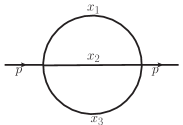
(b)

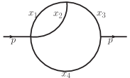
(c)

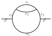
(d)

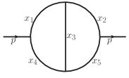
Figure 2: 2-loop self-energy diagrams with massive internal lines: (a) 2-loop sunrise-sunset $N=3$ (Laporta [1] , Fig 2(b)), (b) 2-loop lemon $N=4$ (Laporta [1] , Fig 2(c)), (c) 2-loop half-boiled egg $N=5$, (d) 2-loop Magdeburg $N=5$ ((Laporta [1] , Fig 2(d))

.

Analytic results for the integrals have been derived by many authors. We use the following formulas for the functions $U$ and $V$ in Eq (4):
$-$ for the sunrise-sunset diagram (Fig 2(d)(a)), $U=x_{1}x_{2}+x_{2}x_{3}+x_{3}x_{1},\leavevmode\nobreak\ W/s=x_{1}x_{2}x_{3};$
$-$ for the lemon diagram (Fig 2(d)(b)), we have $U=x_{12}x_{34}+x_{1}x_{2},\leavevmode\nobreak\ W/s=x_{4}\,(x_{1}x_{2}+x_{2}x_{3}+x_{3}x_{1});$
$-$ for the half-boiled egg diagram (Fig 2(d)(c)), $U=x_{12}x_{345}+x_{1}x_{2},\leavevmode\nobreak\ W/s=x_{5}\,(x_{12}x_{34}+x_{1}x_{2});$
$-$ for the Magdeburg diagram (Fig 2(d)(d)), $U=x_{14}x_{25}+x_{3}x_{1245},\leavevmode\nobreak\ W/s=x_{1}x_{4}x_{235}+x_{2}x_{5}x_{134}+x_{3}\,(x_{1}x_{5}+x_{2}x_{4}).$

In the numerical evaluation, we take particular values for energy and masses, i.e., $s=p^{2}=1,$ and all masses $m_{r}=1$ in order to make comparisons with results in the references.

The integrals are expanded with respect to the dimensional regularization parameter $\varepsilon.$ The integrals $I_{a}^{S2},I_{b}^{S2}$ are divergent as $\displaystyle{1/\varepsilon^{2}},$ which is the product of $\displaystyle{1/\varepsilon}$ from the $\Gamma$-function part and $\displaystyle{1/\varepsilon}$ from the integral part. The integral $I_{c}^{S2}$ is divergent as $\displaystyle{1/\varepsilon},$ which comes from the integral part. The integral $I_{d}^{S2}$ is finite. The expansions are of the form of Eq (3),

$${\color[rgb]{0,0,0}S(\varepsilon)\sim\sum_{k\geq\kappa}C_{k}\,\varepsilon^{k}\leavevmode\nobreak\ \leavevmode\nobreak\ \leavevmode\nobreak\ \leavevmode\nobreak\ \leavevmode\nobreak\ \leavevmode\nobreak\ \mbox{as\leavevmode\nobreak\ \leavevmode\nobreak\ }\varepsilon\rightarrow 0},$$ (17)

and we use linear extrapolation to approximate the coefficients of the leading terms. We multiply the integrals $I_{a}^{S2},$ $I_{b}^{S2}$ and $I_{d}^{S2}$ of Eq (4) with the factor $\Gamma(1+\varepsilon)^{-2}$ for comparison with the results in Laporta [1], since the latter are computed with this factor. The half-boiled egg diagram is not covered in [1]. We give the analytic formula for $J_{c}^{S2}$ in Appendix A of this paper.

$$I_{a}^{S2}({\varepsilon})\leavevmode\nobreak\ \Gamma(1+{\varepsilon})^{-2}=\sum_{k\geq-2}C_{k}\,{\varepsilon^{k}} = -1.5\,{\varepsilon^{-2}}-4.25\,{\varepsilon^{-1}}-7.375-17.22197253479\,{\varepsilon}\ldots$$ (18)

$$I_{b}^{S2}({\varepsilon})\leavevmode\nobreak\ \Gamma(1+{\varepsilon})^{-2}=\sum_{k\geq-2}C_{k}\,{\varepsilon^{k}} = 0.5\,{\varepsilon^{-2}}+0.6862006357658\,{\varepsilon^{-1}}-0.6868398873414$$ (19)

$$+ 1.486398391913\,{\varepsilon}\ldots$$

$$J_{c}^{S2}({\varepsilon})=\sum_{k\geq-1}C_{k}\,{\varepsilon^{k}} = 0.6045997880781\,{\varepsilon^{-1}}-0.1756970002260\,-0.2977242542666\,{\varepsilon}$$ (20)

$$+ 0.4140155361099\,{\varepsilon^{2}}\ldots$$

$$I_{d}^{S2}({\varepsilon})\leavevmode\nobreak\ \Gamma(1+{\varepsilon})^{-2}=\sum_{k\geq 0}C_{k}\,{\varepsilon^{k}} = 0.9236318265199-1.284921671848\,{\varepsilon}+2.689507626490\,{\varepsilon^{2}}$$ (21)

$$- 5.338399227511\,{\varepsilon^{3}}\ldots$$

Note that the value of $\kappa$ in Eq (17) corresponds with the index of the first coefficient $C_{\kappa}$ in the expansion. In that case we find that, if $\kappa$ is replaced by $\kappa-1$ for the extrapolation, then the first coefficient converges to $C_{\kappa-1}=0.$

Table 1: Results UV sunrise-sunset integral, $I_{a}^{S2}\,\Gamma(1+\varepsilon)^{-2}$  (on Mac Pro),  rel. err. tol. $t_{r}=10^{-9}$ (outer), $10^{-9}$ (inner), $T[s]$ = Time (elapsed user time in $s$),  $\varepsilon=1.2^{-10-\ell}$ (starting at $1.2^{-10}$),  $E_{r}=$ outer integration estim. rel. error

	Integral  $I_{a}^{S2}\,\Gamma(1+\varepsilon)^{-2}$  Extrapolation
$\ell$	$E_{r}$	T[s]	Res.  $C_{-2}$	Res.  $C_{-1}$	Res.  $C_{0}$	Res.  $C_{1}$
$0$	3.2e-10	0.015
$1$	4.7e-10	0.013	-1.156740414	-8.2070492
$2$	6.6e-10	0.013	-1.603088981	-2.1269693	-20.5343
$3$	9.2e-10	0.013	-1.476861131	-4.9718825	0.60362	-51.7769
$4$	4.0e-11	0.028	-1.504342324	-4.0584835	-10.6252	8.73336
$5$	6.9e-11	0.029	-1.499360223	-4.2880409	-6.46343	-28.3731
$6$	1.3e-10	0.029	-1.500078550	-4.2438757	-7.57341	-13.7781
$7$	2.2e-10	0.028	-1.499992106	-4.2507887	-7.34157	-18.0041
$8$	3.6e-10	0.028	-1.500000763	-4.2499043	-7.38015	-17.0657
$9$	5.4e-10	0.029	-1.499999886	-4.2500174	-7.37374	-17.2650
$10$	7.8e-10	0.029	-1.500000026	-4.2499948	-7.37544	-17.2010
Eq (18):			-1.5	-4.25	-7.375	-17.2220

Table 2: Results UV lemon integral, $I_{b}^{S2}\,\Gamma(1+\varepsilon)^{-2}$  (on Mac Pro),  rel. err. tol. $t_{r}=10^{-10}$ (outer), $5\times 10^{-11}$ (inner two), $T[s]$ = Time (elapsed user time in $s$),  $\varepsilon=1/b_{\ell}$ (starting at 1/4),  $E_{r}=$ outer integration estim. rel. error

	Integral  $I_{b}^{S2}\,\Gamma(1+\varepsilon)^{-2}$  Extrapolation
$b_{\ell}$	$E_{r}$	T[s]	Res.  $C_{-2}$	Res.  $C_{-1}$	Res.  $C_{0}$	Res.  $C_{1}$
$4$	3.5e-11	0.36
$6$	8.8e-11	0.34	0.5130221162587	0.52467607220
$8$	2.9e-12	0.40	0.5031467341833	0.62342989295	-0.237009170
$12$	3.4e-12	0.41	0.5004379328119	0.67218831764	-0.518724512	0.52008986
$16$	1.5e-11	0.39	0.5000485801347	0.68386889795	-0.643317369	1.08075772
$24$	4.7e-11	0.38	0.5000037328535	0.68593187289	-0.679195194	1.37495588
$32$	4.1e-11	0.43	0.5000002195177	0.68617780639	-0.685884585	1.46545941
$48$	1.4e-11	0.44	0.5000000087538	0.68619930431	-0.686757991	1.48373011
$64$	1.3e-11	0.31	0.5000000002937	0.68620057333	-0.686834471	1.48614633
$96$	3.2e-11	0.31	0.5000000000039	0.68620063534	-0.686839872	1.48639673
Eq (19):			0.5	0.68620063577	-0.686839887	1.48639839

Table 3: Results UV half-boiled egg integral, $J_{c}^{S2}$  (on Mac Pro),  rel. err. tol. $t_{r}=10^{-12}$ (outer), $5\times 10^{-13}$ (inner three), $T[s]$ = Time (elapsed user time in $s$),  $\varepsilon=1/b_{\ell}$ (starting at 1.0),  $E_{r}=$ outer integration estim. rel. error

	Integral  $J_{c}^{S2}$  Extrapolation
$b_{\ell}$	$E_{r}$	T[s]	Res.  ${C}_{-1}$	Res.  ${C}_{0}$	Res.  ${C}_{1}$	Res.  ${C}_{2}$
$1$	4.2e-13	7.3
$2$	3.9e-14	11.4	0.6121795323700	-0.26893337928
$3$	2.6e-13	10.8	0.6219220162954	-0.29816083105	-0.019484967
$4$	5.2e-13	10.3	0.6084345649676	-0.21723612309	-0.128876997	0.08092471
$6$	1.1e-13	14.9	0.6050661595977	-0.18355206939	-0.246771185	0.24934498
$8$	7.9e-13	9.2	0.6046439346384	-0.17679647004	-0.286882556	0.35912347
$12$	9.6e-13	12.5	0.6046028724387	-0.17581097725	-0.296039426	0.40100691
$16$	2.3e-13	19.4	0.6045999612478	-0.17570617438	-0.297527045	0.41176667
$24$	8.7e-13	19.1	0.6045997948488	-0.17569752162	-0.297707921	0.41374216
$32$	7.7e-13	24.9	0.6045997882885	-0.17569702304	-0.297723238	0.41399119
$48$	4.1e-13	33.2	0.6045997880782	-0.17569700033	-0.297724241	0.41401488
Eq (20):			0.6045997880781	-0.17569700023	-0.297724254	0.41401554

Table 4: Results UV Magdeburg integral, $I_{d}^{S2}\,\Gamma(1+\varepsilon)^{-2}$  (by ParInt on thor in long double precision),  rel. err. tol. $t_{r}=10^{-13},$ max. # evals = 1B, $T[s]$ = Time (elapsed user time in $s$),  $\varepsilon=2^{-\ell}$ (starting at 1.0),  $E_{r}=$ estim. rel. error

	Integral  $I_{d}^{S2}\,\Gamma(1+\varepsilon)^{-2}$  Extrapolation
$\ell$	$E_{r}$	T[s]	Res.  $C_{0}$	Res.  $C_{1}$	Res.  $C_{2}$	Res.  $C_{3}$
$0$	8.5e-14	0.8
$1$	1.0e-13	19.7	0.69130084611470	-0.142989490499
$2$	1.6e-13	7.5	0.84949643770104	-0.617576265258	0.3163911832
$3$	4.8e-13	6.9	0.90878784906010	-1.032616144771	1.1464709422	-0.47433129
$4$	8.5e-13	6.6	0.92198476262012	-1.230569848171	2.0702548914	-2.05796092
$5$	1.2e-12	6.5	0.92353497740505	-1.278626506507	2.5508214747	-3.98022725
$6$	3.0e-12	6.6	0.92362889210499	-1.284543132600	2.6730984140	-5.02831530
$7$	2.4e-12	6.6	0.92363178137723	-1.284910070175	2.6885097922	-5.30131686
$8$	2.8e-12	6.6	0.92363182617006	-1.284921492347	2.6894768694	-5.33613164
$9$	2.8e-12	6.6	0.92363182651847	-1.284921670382	2.6895071354	-5.33832809
$10$	2.9e-12	6.6	0.92363182651995	-1.284921671903	2.6895076534	-5.33840357
$11$	2.9e-12	6.6	0.92363182651990	-1.284921671790	2.6895075765	-5.33838110
$12$	2.9e-12	6.6	0.92363182651992	-1.284921671898	2.6895077252	-5.33846839
$13$	3.7e-12	6.6	0.92363182651991	-1.284921671798	2.6895075774	-5.33835823
$14$	2.9e-12	6.6	0.92363182651991	-1.284921671840	2.6895076182	-5.33839951
Eq (21):			0.9236318265199	-1.284921671848	2.6895076265	-5.33839923

Tables 1,  2,  3 and  4 show the convergence of the extrapolation method for the integrals of Eqs (18)-(21). While the integral $I_{d}^{S2}$ has no UV-divergent terms and starts from a finite term ($\kappa=0$), the coefficients ${C}_{0}$, ${C}_{1}$, ${C}_{2}$ and ${C}_{3}$ can be obtained using extrapolation. To evaluate $I_{d}^{S2}$, we transform the variables as:

$$x_{1} = y_{1m}y_{3m}y_{4},\leavevmode\nobreak\ \leavevmode\nobreak\ \leavevmode\nobreak\ \leavevmode\nobreak\ \leavevmode\nobreak\ \leavevmode\nobreak\ x_{2}\leavevmode\nobreak\ =\leavevmode\nobreak\ y_{1m}y_{3m}y_{4m},$$

$$x_{3} = y_{1}y_{2m},\leavevmode\nobreak\ \leavevmode\nobreak\ \leavevmode\nobreak\ \leavevmode\nobreak\ \leavevmode\nobreak\ \leavevmode\nobreak\ x_{4}\leavevmode\nobreak\ =\leavevmode\nobreak\ y_{1m}y_{3},$$ (22)

$$x_{5} = y_{1}y_{2}$$

with $y_{im}=1-y_{i}$ and Jacobian $y_{1}y_{1m}^{2}y_{3m}$. The accuracy and time of the calculation of the integral sequence for the extrapolation in Table 4 are improved considerably by the transformation.

For the first three integrals, an iterated integration is applied with Dqags from Quadpack, on a Mac Pro, 2.6 GHz Intel Core i7, with 16 GB memory, under OS X. The value of $E_{r}$ is (the absolute value of) the estimated relative error returned by the outer integration (not accounting for the inner integration error). It is listed for each integration, as well as the elapsed user time $T[s]$ (in seconds). The time for the extrapolation is negligible compared to that of the integration. We use a standard linear system solver to solve very small systems (of sizes $2\times 2$ up to around $15\times 15$ for the cases in this paper).

Table 4 illustrates an application of ParInt for the Magdeburg integral, on the thor system of the High Performance Computing and Big Data Center at WMU, with dual Intel Xeon E5-2670, 2.6 GHz processors, 16 cores and 128 GB of memory per node. For the distributed computation with ParInt, using 16 processes per node and 64 processes total, the MPI host file has four lines of the form nx slots=16 where nx represents a selected node name. The running time is reported (in seconds) from ParInt, and comprises all computation not inclusive of the process spawning and ParInt initialization at the start of the program. The cubature rule of degree 9 is used for integration over the subregions (see Section 3.2), to an allowed maximum number of one billion (1B) integrand evaluations over all processes, and a requested accuracy of $t_{r}=10^{-13}$ in long double precision. The total estimated relative error is denoted by $E_{r}$ in Table 4.

The extrapolation parameter for Tables 2 and 3 adheres to $\{1/b_{\ell}\}$ where $\{b_{\ell}\}$ is the Bulirsch sequence [29] started at an early index. Tables 1 and 4 give results for a geometric sequence of the extrapolation parameter $\varepsilon=\varepsilon_{\ell}.$ The convergence results in Tables 1-2 and 4 are compared with with the expansion coefficients available from [1] (see Eqs (18)-(19), (21). Table 3 shows excellent approximations to the analytic result of Eq (20) derived in the Appendix.

Throughout the extrapolation we keep track of the difference with the previous result as a measure of convergence. Increases of the distance between successive extrapolation results are an indicator that the convergence is no longer improving and the procedure can be terminated.

4.2 2-loop vertex integrals

(a)

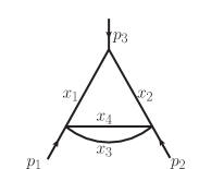
(b)

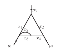
Figure 3: 2-loop vertex (UV-divergent) diagram with massive internal lines: (a) $N=4$ (Laporta [1] , Fig 3(b) ), (b) $N=5$ (Laporta [1] , Fig 3(c) )

Fig 3(a) and (b) depict 2-loop vertex diagrams with $N=4$ and $5$ internal lines, and the integrals of Eq (4) are denoted by $I_{a}^{V2}$ and $I_{b}^{V2}$, respectively. The former is divergent as $\displaystyle{1/\varepsilon^{2}},$ which is the product of $\displaystyle{1/\varepsilon}$ arising from the $\Gamma$-function factor and $\displaystyle{1/\varepsilon}$ from the integral. The latter is divergent as $\displaystyle{1/\varepsilon}$ arising from the integral.
$-$ For $I_{a}^{V2}$, we have $U=x_{12}x_{34}+x_{3}x_{4}$ and $W=p_{1}^{2}x_{1}x_{3}x_{4}+p_{2}^{2}x_{2}x_{3}x_{4}+p_{3}^{2}x_{1}x_{2}x_{34}.$
$-$ For $I_{b}^{V2}$, we have $U=x_{124}x_{3}+x_{1234}x_{5}$ and $W=(p_{1}^{2}x_{1}+p_{2}^{2}x_{2})\,(x_{3}x_{45}+x_{4}x_{5})+p_{3}^{2}x_{1}x_{2}x_{35}$.

Table 5: Results UV vertex integral, $I_{a}^{V2}$  (on Mac Pro),  rel. err. tol. $t_{r}=10^{-10}$ (outer), $5\times 10^{-11}$ (inner three), $T[s]$ = Time (elapsed user time in $s$),  $\varepsilon=1/b_{\ell}$ (starting at 1/3),  $E_{r}=$ outer integration estim. rel. error

	Integral ${I}_{a}^{V2}\leavevmode\nobreak\ \Gamma(1+\varepsilon)^{-2}$  Extrapolation
$b_{\ell}$	$E_{r}$	T[s]	Res.  ${C}_{-2}$	Res.  ${C}_{-1}$	Res.  ${C}_{0}$	Res.  ${C}_{1}$
$3$	8.7e-12	$1.4$
$4$	2.3e-11	$1.5$	0.51489021736	0.535680679
$6$	3.1e-10	$1.8$	0.50586162735	0.598880809	-0.1083431
$8$	8.2e-11	$5.2$	0.50111160609	0.660631086	-0.3648442	0.342002
$12$	1.2e-09	$2.5$	0.50015901670	0.680635463	-0.5153534	0.822107
$16$	1.7e-09	$4.2$	0.50001764652	0.685300679	-0.5733151	1.161395
$24$	4.4e-09	$20.5$	0.50000135665	0.686098882	-0.5885950	1.307352
$32$	7.7e-09	$19.1$	0.50000007798	0.686192225	-0.5912981	1.347595
$48$	3.8e-10	$8.6$	0.50000000083	0.686200327	-0.5916415	1.355242
Eq   (23):			0.5	0.686200636	-0.5916667	1.356197

Table 6: Results UV vertex integral, $I_{b}^{V2}\,\Gamma(1+\varepsilon)^{-2}$  (by ParInt on thor in long double precision),  rel. err. tol. $t_{r}=10^{-13},$ max. # evals = 10B, $T[s]$ = Time (elapsed user time in $s$),  $\varepsilon=1.2^{-\ell}$ (starting at $1.2^{-8}$),  $E_{r}=$ estim. rel. error

	Integral  $I_{b}^{V2}\,\Gamma(1+\varepsilon)^{-2}$  Extrapolation
$\ell$	$E_{r}$	T[s]	Res.  $C_{-1}$	Res.  $C_{0}$	Res.  $C_{1}$	Res.  $C_{2}$
$8$	9.9e-14	0.7
$9$	5.7e-14	0.9	0.653547537693	0.10873442398
$10$	8.7e-14	1.3	0.667737620294	-0.02549804326	0.148227487
$11$	5.7e-14	1.7	0.670486635108	-0.06852379156	0.536826159	-0.37763368
$12$	9.8e-14	6.9	0.671112937626	-0.08297974141	0.660237921	-0.83947237
$13$	9.8e-14	8.4	0.671231024200	-0.08675821868	0.707808436	-1.13401646
$14$	9.6e-14	9.3	0.671250129509	-0.08757395495	0.722045637	-1.26401791
$15$	9.4e-14	10.3	0.671252763777	-0.08772025175	0.725452770	-1.30714663
$16$	1.0e-13	65.7	0.671253072371	-0.08774214433	0.726115949	-1.31834841
$17$	9.4e-14	13.8	0.671253102986	-0.08774488225	0.726221896	-1.32067610
$18$	9.9e-14	18.1	0.671253105554	-0.08774516889	0.726235878	-1.32106853
$19$	9.3e-14	39.5	0.671253105741	-0.08774519476	0.726237453	-1.32112425
$20$	1.0e-13	76.0	0.671253105743	-0.08774519512	0.726237480	-1.32112544
$21$	1.0e-13	77.4	0.671253105751	-0.08774519670	0.726237628	-1.32113350
$22$	1.1e-13	77.8	0.671253105748	-0.08774519610	0.726237559	-1.32112888
Eq (24):			0.671253105748	-0.08774519609	0.726237563	-1.32112949

Table 7: Results UV vertex integral, $I_{b}^{V2}\,\Gamma(1+\varepsilon)^{-2}$  (by ParInt on thor in long double precision),  rel. err. tol. $t_{r}=10^{-13},$ max. # evals = 10B, $T[s]$ = Time (elapsed user time in $s$),  $\varepsilon=1.5^{-\ell}$ (starting at 1.0),  $E_{r}=$ estim. rel. error

	Integral  $I_{b}^{V2}\,\Gamma(1+\varepsilon)^{-2}$  Extrapolation
$\ell$	$E_{r}$	T[s]	Res.  $C_{-1}$	Res.  $C_{0}$	Res.  $C_{1}$	Res.  $C_{2}$
$0$	1.0e-13	0.31
$1$	1.0e-13	0.77	0.552646148416	-0.03261093175
$2$	2.7e-14	0.26	0.645884613605	-0.09301315450	0.139857698
$3$	3.9e-14	0.44	0.659977890791	-0.02607008786	0.240272298	-0.04756481
$4$	4.9e-14	0.92	0.668110702931	-0.04000901078	0.428597729	-0.02705818
$5$	1.2e-14	1.32	0.670596883473	-0.07279551667	0.588431945	-0.63020875
$6$	3.8e-14	1.96	0.671155085836	-0.08439565952	0.680218075	-0.98346458
$7$	9.5e-14	13.9	0.671242833695	-0.08721867268	0.715417521	-1.20334533
$8$	1.0e-13	76.5	0.671252362159	-0.08768802398	0.724477468	-1.29252918
$9$	1.0e-13	77.7	0.671253068976	-0.08774095520	0.726041833	-1.31636903
$10$	9.3e-15	26.8	0.671253104515	-0.08774498285	0.726222803	-1.32059155
$11$	2.1e-13	78.3	0.671253105720	-0.08774518885	0.726236811	-1.32108845
$12$	4.9e-13	79.5	0.671253105748	-0.08774519595	0.726237540	-1.32112754
Eq (24):			0.671253105748	-0.08774519609	0.726237563	-1.32112949

In order to compare with Laporta’s results [1], we put $m_{r}=1$ and $p_{1}^{2}=p_{2}^{2}=p_{3}^{2}=1,$ and multiply the integrals with a factor $\Gamma(1+{\varepsilon})^{-2}.$ The expansions from [1] are:

$$I_{a}^{V2}({\varepsilon})\leavevmode\nobreak\ \Gamma(1+{\varepsilon})^{-2}=\sum_{k\geq-2}C_{k}\,{\varepsilon^{k}} = 0.5\,{\varepsilon^{-2}}+0.6862006357658\,{\varepsilon^{-1}}-0.5916667014024$$ (23)

$$+ 1.356196533114\,{\varepsilon}\ldots$$

$$I_{b}^{V2}({\varepsilon})\leavevmode\nobreak\ \Gamma(1+{\varepsilon})^{-2}=\sum_{k\geq-1}C_{k}\,{\varepsilon^{k}} = 0.671253105748\,{\varepsilon^{-1}}-0.08774519609257+0.7262375626947\,{\varepsilon}$$ (24)

$$- 1.32112948587\,{\varepsilon^{2}}\ldots$$

The numerical results for $I_{a}^{V2}$ obtained with iterated integration by Dqags, and extrapolation using a Bulirsch sequence and linear system solver are shown in Table 5. Tables 6-7 show results for $I_{b}^{V2}$ with geometric sequences of base 1/1.2 and 1/1.5, respectively, achieved by ParInt using 64 processes on four 16-core nodes of the thor cluster. Both deliver very accurate results, with the final results in Table 6 slightly closer to the analytic values. The extrapolation in Table 7 converges somewhat faster. For the computation of $I_{b}^{V2}$, we transform the variables as for $I_{d}^{S2}$ in Section 4.1. This transformation maps the integration domain to the 4-dimensional unit cube and also guards against the loss of significant digits near the boundaries.

4.3 2-loop box integrals

The 2-loop box integrals according to Eq (4) for the diagrams in Fig 4 are all finite integrals and can be evaluated with $\varepsilon=0$. Integral approximations obtained with ParInt for the double-triangle ($N=5$), tetragon-triangle ($N=6$), pentagon-triangle ($N=7$), ladder and crossed ladder ($N=7$) diagrams were presented in [18]. The $U$ and $W$ functions can also be found in the reference. In the numerical evaluation, we set $s=t=1,\ p_{j}^{2}=1,\ m_{r}=1$ for simplicity and for comparisons with other results in the literature.

(a)

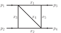
(b)

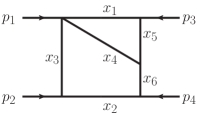
(c)

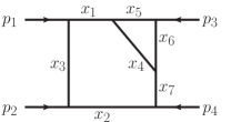
(d)

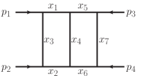
(e)

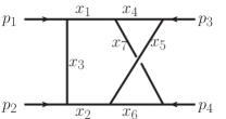
Figure 4: 2-loop box diagrams with massive internal lines (finite diagrams) (a) double-triangle $N=5$ (Laporta [1],  Fig 4(c)), (b) tetragon-triangle $N=6$ (Laporta [1],  Fig 4(d)), (c) pentagon-triangle $N=7$ (Laporta [1],  Fig 4(g)), (d) ladder $N=7$ (Laporta [1],  Fig 4(h)), (e) crossed ladder $N=7$ (Laporta [1],  Fig 4(i))

This subsection provides timing results obtained with ParInt on the thor cluster, corresponding to the five diagrams in Fig 4. Table 8 gives a brief overview of pertinent test specifications, $T_{1},\leavevmode\nobreak\ T_{p}$ and the speedup $S_{p}=T_{1}/T_{p}$ for $p=64.$ The times $T_{p}$ are expressed in seconds, as a function of the number of MPI processes $p,1\leq p\leq 64.$ When referring to numbers of integrand evaluations, million and billion are abbreviated by “M” and “B”, respectively. For instance, the times of the $N=5$ double triangle diagram decrease from 32.6 seconds at $p=1,$ to  0.74 seconds at $p=64$ for $t_{r}=10^{-10}$ (reaching a speedup of 44); whereas the $N=7$ crossed diagram times range between 27.6 seconds and 0.49 seconds for $t_{r}=10^{-7}$ (with speedup exceeding 56). The transformation of Eq (7) was used.

For the two-loop crossed box problem as an example, we ran ParInt in long double precision. The results for an increasing allowed maximum number of evaluations and increasingly strict (relative) error tolerance $t_{r}$ (using 64 processes) are given in Table 9, as well as the corresponding double precision results. Listed are: the integral approximation, relative error estimate $E_{r},$ number of function evaluations reached and time taken in long double precision, followed by the relative error estimate, number of function evaluations reached and running time in double precision. For a comparable number of function evaluations, the time using long doubles is slightly less than twice the time taken using doubles. The iflag parameter returns 0 when the requested accuracy is assumed to be achieved, and 1 otherwise. Reaching the maximum number of evaluations results in abnormal termination with iflag = 1. The integral approximation for the double computation is not listed in Table 9; it is consistent with the long double result within the estimated error (which appears to be over-estimated). Using doubles the program terminates abnormally for the requested relative accuracy of $t_{r}=10^{-10}.$ Normal termination is achieved in this case around 239B evaluations with long doubles.

Fig 5 shows ParInt timing plots for the diagrams of Fig 4, depicting a considerable time decrease as a function of the number of processes $p.$ Plots with similar orders of the time are grouped in Fig 5(a) and in Fig 5(b).

Timing results obtained with parallel (multi-threaded) iterated integration were given in [18].

Table 8: Test specifications and range of times in Fig 5(a)-(d)

Diagram	Figure/Timing Plot	$N$	Rel Tol	Max evals	$T_{1}[s]$	$T_{64}[s]$	Speedup
			$E_{r}$				$S_{p}$ for $p=64$
double triangle	Fig 4(a) / Fig 5(a)	5	$10^{-10}$	400M	32.6	0.74	44.1
crossed ladder	Fig 4(e) / Fig 5(a)	7	$10^{-7}$	300M	27.6	0.49	56.3
tetragon triangle	Fig 4(b) / Fig 5(b)	6	$10^{-9}$	3B	213.6	5.06	42.2
ladder	Fig 4(d) / Fig 5(b)	7	$10^{-8}$	2B	189.9	4.33	43.9
pentagon triangle	Fig 4(c) / Fig 5(c)	7	$10^{-8}$	5B	507.9	8.83	57.5
crossed ladder	Fig 4(e) / Fig 5(d)	7	$10^{-9}$	20B	1892.5	34.6	54.7

Table 9: ParInt long double and double results for crossed diagram Fig 4(e)

$t_{r}$	Max	long double precision					double precision
	Evals	Integral Approx	$E_{r}$	iflag	#Evals	Time[s]	$E_{r}$	iflag	#Evals	Time
$10^{-08}$	600M	0.085351397048123	3.5e-07	1	600000793	1.7	3.4E-07	1	600001115	0.95
	1B	0.085351397753978	1.7e-07	1	1000000141	2.9	1.6e-07	1	1000000141	1.6
	2B	0.085351398064779	2.9e-08	1	2000000443	6.0	2.9e-08	1	2000000765	3.3
	6B	0.085351398130559	5.6e-09	0	4164032999	14.3	8.0e-09	0	4424455329	8.6
$10^{-09}$	10B	0.085351398143465	5.5e-09	1	10000001571	29.7	5.5e-09	1	10000000927	16.4
	50B	0.085351398152623	9.9e-10	0	35701321579	124.4	4.5e-10	0	9799638359	16.0
$10^{-10}$	80B	0.085351398153315	5.5e-10	1	80000001137	240.2	5.5e-10	1	80000000171	133.5
	100B	0.085351398153507	4.1e-10	1	100000000093	302.0	4.1e-10	1	100000000093	168.3
	300B	0.085351398153798	9.1e-11	0	238854968513	642.3	1.3e-10	1	300000000279	587.2

(a)

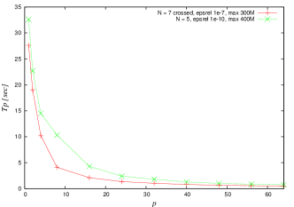
(b)

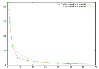
(c)

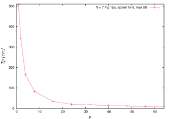
(d)

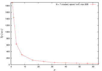
Figure 5: ParInt timing plots for Fig 4 diagrams as a function of the number of procs. $p.$ (a) $N=5$ [Fig 4(a)], $t_{r}=10^{-10}$ and $N=7$ [Fig 4(e)], $t_{r}=10^{-7};$ (b) $N=6$ [Fig 4(b)], $t_{r}=10^{-8}$ and $N=7$ [Fig 4(d)], $t_{r}=10^{-8};$ (c) $N=7$ [Fig 4(c)], $t_{r}=10^{-8};$ (d) $N=7$ [Fig 4(e)], $t_{r}=10^{-9}$

5 3-loop self-energy integrals

In this section we deal with the integral determined by Eq (5) for $L=3$ and $n=4-2\varepsilon,$

$$I=(-1)^{N}{\Gamma\left(N-6+3\varepsilon\right)}\int_{0}^{1}\prod_{r=1}^{N}dx_{r}\,\delta(1-\sum x_{r})\frac{1}{U^{2-\varepsilon}(V-i\varrho)^{N-6+3\varepsilon}}.$$ (25)

UV divergence occurs when $U$ vanishes at the boundaries. The $\Gamma$-function in Eq (25) contributes to UV divergence when $N\leq 6$. As shown in the figures, the entering momentum is $p,$ and we denote $s=p^{2}$.

We calculate integrals adhering to Eq (25), denoted by $I_{a}^{S3},\,I_{b}^{S3},\,\cdots,I_{j}^{S3},$ for the diagrams of Fig 6(a)-(j), respectively. In the following four subsections, we consider massless/massive internal lines and UV finite/divergent cases.

5.1 3-loop finite integrals with massless internal lines

The integrals $I_{a}^{S3},\,I_{b}^{S3},\,I_{c}^{S3},\,I_{d}^{S3}$ are finite, with the $U,\ W$ functions given in Eqs (26)-(29) below.

$$\mathrm{(a)}\quad\left\{\begin{array}[]{l}U=x_{4}x_{7}x_{12356}+x_{12}x_{47}x_{56}+x_{3}\,(x_{12}x_{4}+x_{56}x_{7}+x_{12}x_{56})\\ W/s=x_{4}x_{7}x_{15}x_{236}+x_{4}\,(x_{1}x_{2}x_{356}+x_{12}x_{36}x_{5})\\ \quad+x_{7}\,(x_{5}x_{6}x_{123}+x_{1}x_{23}x_{56})+x_{3}\,(x_{1}x_{2}x_{56}+x_{12}x_{5}x_{6})\end{array}\right.$$ (26)

$$\mathrm{(b)}\quad\left\{\begin{array}[]{l}U=x_{7}\,(x_{12}x_{3456}+x_{34}x_{56})+x_{13}x_{24}x_{56}+x_{1}x_{2}x_{34}+x_{12}x_{3}x_{4}\\ W/s=x_{7}\,(x_{15}x_{26}x_{34}+x_{1}x_{2}x_{56}+x_{12}x_{5}x_{6})+(x_{1}x_{3}+x_{13}x_{5})\,(x_{2}x_{4}+x_{2}x_{6}+x_{4}x_{6})\end{array}\right.$$ (27)

$$\mathrm{(c)}\quad\left\{\begin{array}[]{l}U=x_{5}x_{8}x_{123467}+x_{5}x_{12}x_{3467}+x_{8}x_{1234}x_{67}+x_{12}x_{34}x_{67}\\ W/s=x_{5}x_{8}x_{136}x_{247}+x_{5}\,(x_{1}x_{2}x_{3467}+x_{12}x_{36}x_{47})\\ \quad+x_{8}\,(x_{6}x_{7}x_{1234}+x_{13}x_{24}x_{67})+x_{1}x_{2}x_{34}x_{67}+x_{12}x_{3}x_{4}x_{67}+x_{12}x_{34}x_{6}x_{7}\end{array}\right.$$ (28)

$$\mathrm{(d)}\quad\left\{\begin{array}[]{l}U=x_{5}x_{8}x_{123467}+x_{5}x_{124}x_{367}+x_{8}x_{123}x_{467}+x_{12}x_{3}x_{467}+x_{123}x_{4}x_{67}\\ W/s=x_{5}x_{8}x_{136}x_{247}+x_{5}\,(x_{17}x_{24}x_{36}+x_{1}x_{7}x_{2346})\\ \quad+x_{8}\,(x_{26}x_{13}x_{47}+x_{2}x_{6}x_{1347})+x_{34}\,(x_{1}x_{2}x_{67}+x_{12}x_{6}x_{7})+x_{3}x_{4}x_{17}x_{26}\end{array}\right.$$ (29)

In this subsection we take $m_{r}=0$ for the internal lines. In the absence of divergences we set $\varrho=\varepsilon=0$ in Eq (25) for $I_{a}^{S3},\,I_{b}^{S3},\,I_{c}^{S3},$ and show the results in Table 10. However, the integral $I_{d}^{S3}$ is problematic with $\varrho=\varepsilon=0$ in view of integrand singularities, and we use the extrapolation method with either $\varepsilon=0$ and in the limit as $\rho\rightarrow 0,$ or with $\varrho=0$ and in the limit as $\varepsilon\rightarrow 0.$ The analytic result is the same for the four diagrams (see [2]),

$$I_{a}^{S3}=I_{b}^{S3}=I_{c}^{S3}=I_{d}^{S3}=20\,\zeta_{5}=20.738555102867\ldots\,.$$

(a)

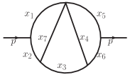
(b)

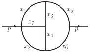
(c)

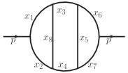
(d)

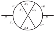
(e)

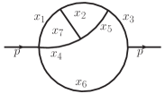
(f)

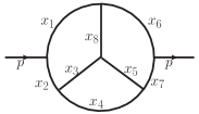
(g)

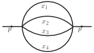
(h)

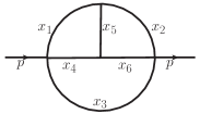
(i)

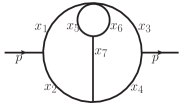
(j)

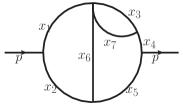
Figure 6: 3-loop self-energy diagrams with massive and massless internal lines (finite and UV-divergent diagrams), cf. Laporta [1], Baikov and Chetyrkin [2]: (a) $N=7$, (b) $N=7$, (c) $N=8$, (d) $N=8$, (e) $N=7$, (f) $N=8$, (g) $N=4$, (h) $N=6$, (i) $N=7$, (j) $N=7$

ParInt numerical results and timings were given in [49] for the 3-loop diagrams of Fig 6(a)-(d), from runs on 16-core nodes of the thor cluster. For the integration over each subregion, the rule of degree 9 is used (see Section 3.2), which evaluates the 6D integrand at 453 points and the 7D integrand at 717 points. These integrals are transformed to the unit cube according to Eq (7). Table 10 lists the results obtained directly with $\varrho=\varepsilon=0$ for Fig 6(a)-(c) by ParInt using 48 processes: integral approximation, relative error estimate $E_{r},$ and time in seconds for various total numbers of function evaluations in double and long double precision. Fig 7 shows times and speedups as a function of the number of processes $p,$ for a computation of the integrals of Fig 6(a)-(c) using 10B integrand evaluations in double precision. Denoting the time in seconds for $p$ processes by $T_{p}[s],$ the corresponding speedup given by $S_{p}=T_{1}/T_{p}$ is nearly optimal – which would coincide with the diagonal in the graph, or slightly superlinear ($>p$) over the given range of $p.$

Table 10: ParInt accuracy and times with 48 procs. for loop integrals of Fig 6(a)-(c) with massless internal lines, using  $\varrho=0,$  and various numbers of function evaluations; $E_{r}=$ integration estim. rel. error

		double precision			long double precision
Diagram	# Fcn.	Integral	Rel. err.	Time	Integral	Rel. err.	Time
	Evals.	Result	Est. $E_{r}$	T[s]	Result	Est. $E_{r}$	T[s]
Exact:		20.73855510			20.73855510
Fig 6 (a)	5B	20.73871652	2.21e-05	9.0	20.73871522	2.5e-05	16.0
	10B	20.73856839	3.50e-06	17.9	20.73856878	3.42e-06	32.1
	25B	20.73855535	3.79e-07	44.9	20.73855539	3.71e-07	80.5
	50B	20.73855508	9.07e-08	90.3	20.73855508	8.94e-08	161.1
	75B	20.73855507	4.26e-08	135.6	20.73855507	4.23e-08	242.1
	100B	20.73855508	2.59e-08	180.8	20.73855508	2.56e-08	323.2
Fig 6 (b)	5B	20.73933800	3.69e-05	9.7	20.73933292	3.63e-05	17.5
	10B	20.73872210	6.64e-06	19.4	20.73872078	6.61e-06	35.1
	25B	20.73857098	8.32e-07	48.6	20.73857018	8.12e-07	87.9
	50B	20.73855716	1.96e-07	98.2	20.73855718	1.95e-07	175.9
	75B	20.73855576	9.28e-08	146.4	20.73855575	9.12e-08	264.4
	100B	20.73855540	5.68e-08	196.7	20.73855540	5.43e-08	352.6
Fig 6 (c)	5B	20.74194961	1.19e-03	10.3	20.74196270	1.19e-03	19.6
	10B	20.73886434	3.64e-04	20.7	20.73880437	3.51e-04	39.2
	25B	20.73827908	5.04e-05	51.7	20.73827607	5.04e-05	98.2
	50B	20.73841802	1.09e-05	103.4	20.73842495	9.79e-06	196.7
	75B	20.73848662	3.66e-06	146.4	20.73848624	3.70e-06	295.0
	100B	20.73851402	1.96e-06	207.5	20.73851338	1.98e-06	393.9

(a)

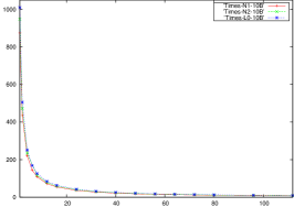
(b)

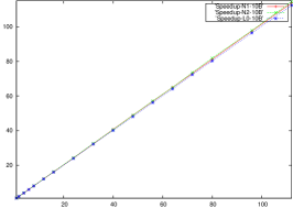
Figure 7: ParInt parallel performance for computation of integrals (Fig 6(a-c)) using 10B evaluations: (a) Computation times (in seconds), (b) $S_{peedup}=T_{1}/T_{p}$

Table 11: Integration with ParInt using 64 procs., max. # evals = 150B, $\varrho=\varrho_{\ell}=2^{-\ell},\ell=20,21,\ldots$ and extrapolation with $\epsilon$-algorithm for Fig 6(d) integral with massless internal lines

	Integral Fig 6(d)			Extrapolation
$\ell$	Integral	$E_{r}$	T[s]	Last	Selected
20	19.69036128576084	1.44e-07	474.5
21	19.91633676759658	1.64e-07	474.6
22	20.09256513888053	1.84e-07	474.7	20.71685142	20.71685142
23	20.23033834092921	1.94e-07	474.7	20.72393791	20.72393792
24	20.33827222472266	2.16e-07	474.7	20.73801873	20.73801873
25	20.42297783943613	2.36e-07	474.7	20.73801873	20.73801873
26	20.48955227010659	2.53e-07	474.7	20.73815511	20.73815511
27	20.54194208640818	2.74e-07	474.7	20.73825979	20.73825979
28	20.58321345028519	2.95e-07	474.7	20.73811441	20.73811441
29	20.61575568045697	3.14e-07	474.8	20.74104946	20.73840576
30	20.64143527978811	3.34e-07	474.6	20.73854289	20.73833347
31	20.66171281606668	3.51e-07	474.7	20.73861767	20.73855952
32	20.67774379215522	4.16e-07	474.6	20.73855567	20.73847582
			Eq (5.1):	20.73855510	20.73855510

With $\varrho=0$ the integrand has boundary singularities. For example, the integrals of Fig 6(a)-(d) have a zero denominator with $U=0$  at  $x_{2}=1$ and the other variables 0 (on the boundary of the unit simplex). Thus the integrand program codes test for zero denominators. However some of the computations overflow by integrand evaluations in the vicinity of the singularities, which is found to occur for Fig 6 (d) in double precision at 1B = $10^{9}$ evaluations or higher.

Table 12: Integration with ParInt using 64 procs., max. # evals = 100B, $\varepsilon=\varepsilon_{\ell}=2^{-\ell},\ell=8,9,\ldots$ and extrapolation with $\epsilon$-algorithm for Fig 6(d) integral with massless internal lines

	Integral Fig 6(d)			Extrapolation
$\ell$	Integral	$E_{r}$	T[s]	Last	Selected
8	21.21987706233486	8.84e-08	648.5
9	20.97727482739239	8.69e-08	648.0
10	20.85743468356065	8.61e-08	649.0	20.74044694	20.74044693
11	20.79787566374119	8.56e-08	647.7	20.73903010	20.73903010
12	20.76818590083646	8.53e-08	648.1	20.73855734	20.73855734
13	20.75336343266232	8.39e-08	648.3	20.73855626	20.73855626
14	20.74595780282081	8.29e-08	647.6	20.73855580	20.73855580
15	20.74225639032920	8.21e-08	647.6	20.73855592	20.73855592
			Eq (5.1):	20.73855510	20.73855510

For the integral $I_{d}^{S3},$ we first take $\varepsilon=0$ and use the following form with non-zero $\varrho:$

$$\Re{e}\,I_{d}^{S3}={\Gamma\left(2\right)}\int_{0}^{1}\prod_{r=1}^{8}dx_{r}\,\delta(1-\sum x_{r})\frac{V^{2}-\varrho^{2}}{U^{2}(V^{2}+\varrho^{2})^{2}}.$$ (30)

Table 11 shows an extrapolation as $\varrho\rightarrow 0$ using the $\epsilon$-algorithm of Wynn [19, 20, 21, 22, 23] (see Section 2.2). The $\varrho_{\ell}$ geometric sequence is computed with base 2,  $\varrho_{\ell}=2^{-\ell}$ and the integration is performed in long double precision using 150B evaluation points. The Selected column lists the element along the new lower diagonal that is presumed the best, based on its distance from the neighboring elements as computed by the $\epsilon$-algorithm function from Quadpack. The Last column lists the final (utmost right) element computed in the lower diagonal. Overall the $\epsilon$-algorithm function from Quadpack appears successful at selecting a competitive element as its result for the iteration.

For an extrapolation as $\varepsilon\rightarrow 0$ we set $\varrho=0,$ so that

$$I_{d}^{S3}={\Gamma\left(2+3\varepsilon\right)}\int_{0}^{1}\prod_{r=1}^{8}dx_{r}\,\delta(1-\sum x_{r})\frac{1}{U^{2-\varepsilon}V^{2+3\varepsilon}}.$$ (31)

Baikov and Chetyrkin [2] derive asymptotic expansions in integer powers of  $\varepsilon$  for 3- and 4-loop integrals arising from diagrams with massless propagators. Table 12 gives an extrapolation in $\varepsilon$ for the integral of the Fig 6(d) diagram, using 100B evaluations for the integrations in long double precision. The results show good agreement with the literature [2, 13]. The integrand with $\varrho=0$ in Eq (31) has a singular behavior with $UV=0$ at the boundaries of the domain. The extrapolation converges faster than that with respect to $\varrho$ in Table 11. The times are larger compared to those of Table 11, likely by calling the pow function (in the C programming language) for each integrand evaluation, whereas the integrand of Eq (30) for the $\varrho$ extrapolation can be calculated using only multiplications, divisions, additions and subtractions.

5.2 3-loop finite integrals with massive internal lines

Table 13: Parallel performance of ParInt for 3-loop diagrams of Fig 6 (a)-(f) with massive internal lines, abs. tolerance $t_{a}=5\times 10^{-10},$ and max. number of evaluations = 10B

3-loop	$N$	Result	Result	Result	$T_{1}[s]$	$T_{64}[s]$	$S_{64}$
diag.		Laporta [1]	$p=1$	$p=64$
Fig 6 (a)	7	2.00250004111	2.00250004113	2.0025000412	879.3	13.4	65.6
Fig 6 (b)	7	1.34139924145	1.34139924147	1.3413992416	1026.2	14.4	71.3
Fig 6 (c)	8	0.27960892328	0.2796089227	0.279608920	1019.7	15.9	64.1
Fig 6 (d)	8	0.14801330396	0.1480133036	0.1480133026	976.6	16.4	59.5
Fig 6 (e)	7	1.32644820827	1.326448206	1.32644819	902.7	15.8	57.1
Fig 6 (f)	8	0.18262723754	0.1826272372	0.1826272368	1018.3	15.8	64.4

For a set of 3-loop self-energy diagrams with massive internal lines given in Fig 6 (a)-(f), corresponding numerical results and ParInt performance results are shown in Table 13. The $U,\ W$ functions for (a)-(d) are given in the previous subsection and those for (e) and (f) are listed in Eqs (32)-(33) below.

$$\mathrm{(e)}\quad\left\{\begin{array}[]{l}U=x_{6}x_{7}x_{1245}+x_{7}x_{12}x_{345}+(x_{1}x_{2}+x_{3}x_{7})\,x_{45}+x_{14}x_{25}x_{36}+x_{12}x_{4}x_{5}\\ W/s=x_{6}\,(x_{7}x_{12}x_{345}+(x_{1}x_{2}+x_{3}x_{7})\,x_{45}+x_{12}x_{4}x_{5}+x_{3}x_{14}x_{25})\end{array}\right.$$ (32)

$$\mathrm{(f)}\quad\left\{\begin{array}[]{l}U=(x_{3}x_{5}+x_{5}x_{8}+x_{3}x_{8})\,x_{12467}+x_{5}x_{12}x_{467}+x_{3}x_{124}x_{67}+x_{4}x_{12}x_{67}+x_{4}x_{8}x_{1267}\\ W/s=(x_{3}x_{5}+x_{5}x_{8}+x_{3}x_{8})\,x_{16}x_{247}+x_{5}\,(x_{1}x_{2}x_{467}+x_{12}x_{47}x_{6})\\ \quad+x_{3}\,(x_{1}x_{6}x_{247}+x_{16}x_{24}x_{7})+x_{4}\,(x_{8}x_{16}x_{27}+x_{1}x_{2}x_{67}+x_{12}x_{6}x_{7})\end{array}\right.$$ (33)

In order to compare our integral approximations with Laporta’s [1], we set all masses $m_{r}=1$ and $s=1,$ and furthermore divide the integral by $\leavevmode\nobreak\ \Gamma(1+\varepsilon)^{3}.$ The integrals are transformed from the (unit) simplex to the (unit) cube according to the transformation of Eqs (7) and (8) and the integration is taken over the cube, using a basic integration rule of polynomial degree 9 (see Section 3.2) and a maximum total of 10B evaluations. The function evaluations are distributed over all the processes. The absolute tolerance is $t_{a}=5\times 10^{-10}$ and the maximum number of integrand evaluations is $10B=10^{10}$ (which is reached in producing the results of Table 13).

The results in Table 13 are given for $p=1$ and for $p=64$ MPI processes. $T_{1}$ is the time with one process and $T_{64}$ is the parallel time on the thor cluster with $p=64$ processes, distributed over four 16-core, 2.6 GHz compute nodes and using the Infiniband interconnect for message passing via MPI. The speedup $S_{64}=T_{1}/T_{64}$ indicates good scalability of the parallel implementation (see also [50, 35]). Note that superlinear speedups ($S_{64}$) are obtained in some cases, where the speedup exceeds the number of processes. This is partially due to the fact that the timing is done within ParInt after the processes are started. It may also be noted that the adaptive partitioning reaches somewhat more accuracy sequentially. Each process has its own priority queue, keyed with the absolute error estimates over their region. This may lead to unnecessary work by the processes locally, which increases with the number of processes.

Tables 14 and 17 are computed with consecutive calls to

i_integrate() } in
a loo

and linear extrapolation, for the functions depicted in Fig 6(b) and (f), respectively. The values of $C_{0},C_{1}$ and $C_{2}$ are listed ($\kappa=0$ in Eq (3)). Results from extrapolation with the $\epsilon$-algorithm are shown in Table 15 for the diagram in Fig 6(b). More extrapolations are needed with the $\epsilon$-algorithm than with linear extrapolation. In this case the latter is more accurate and efficient but utilizes knowledge of the structure of the asymptotic expansion, i.e., that $\varphi_{k}(\varepsilon)=\varepsilon^{k};$ this is not assumed for the non-linear extrapolation with the $\epsilon$-algorithm.

Tables 16 and 18 illustrate the vector function integration capability of ParInt to calculate the entry sequence for the extrapolation (as a vector integral result - see (13)) with one call to i_integrate()}. This rocedure delivers excellent accuracy and efficiency. Note that the integration of the vector function in Table 16 took 2403.4 seconds, compared to the total time of 3766.6 seconds for the integrations listed in Table 14. With regard to Table 18, the time for integrating the vector function was 2180.2 seconds, vs. the total (sum) of 3426.3 seconds for the iterations in Table 17.

Table 14: Integral and leading expansion coefficients using ParInt with 16 procs., and linear extrapolation for 3-loop integral of Fig 6(b),  err. tol. $t_{a}=10^{-12}$; max. # evals = 20B, $\varepsilon=\varepsilon_{\ell}=2^{-\ell},\ell=3,4,\ldots$, $T[s]$ = elapsed time (s); $E_{a}=$ integration estim. abs. error

	Integral Fig 6(b)		Extrapolation
$\ell$	Integral	$E_{a}$	T[s]	Result  $C_{0}$	Result  $C_{1}$	Result  $C_{2}$
${3}$	0.89462319318517	6.33e-10	356.9
${4}$	1.07605987265074	8.56e-10	426.3	1.257496552116	-2.9029868714
${5}$	1.19524813881849	1.15e-09	426.2	1.333416355943	-4.7250621633	9.7177349
${6}$	1.26445377191768	1.34e-09	426.2	1.341017173944	-5.1507079713	16.5280678
${7}$	1.30188593759114	1.46e-09	426.2	1.341390110905	-5.1954604067	18.1988254
${8}$	1.32137252564963	1.52e-09	426.2	1.341399132800	-5.1976978366	18.3778198
${9}$	1.33131707386056	1.55e-09	426.2	1.341399240859	-5.1977522983	18.3868241
${10}$	1.33634079003748	1.57e-09	426.2	1.341399241503	-5.1977529523	18.3870438
${11}$	1.33886565298449	1.58e-09	426.2	1.341399241505	-5.1977529584	18.3870480
Laporta [1]:				1.341399241447	-5.1977529559	18.3870466

Table 15: Integral and leading expansion coefficients using ParInt with 16 procs., and extrapolation with $\epsilon$-algorithm for 3-loop integral of Fig 6(b),  err. tol. $t_{a}=10^{-12}$; max. # evals = 20B, $\varepsilon=\varepsilon_{\ell}=2^{-\ell},\ell=3,4,\ldots$, $T[s]$ = elapsed time (s); $E_{a}=$ integration estim. abs. error

	Integral Fig 6(b)		Extrapolation
$\ell$	Integral	$E_{a}$	T[s]	Result  $C_{0}$	Result  $C_{1}$	Result  $C_{2}$
${3}$	0.89462319318517	6.33e-10	356.9
${4}$	1.07605987265074	8.56e-10	426.3
${5}$	1.19524813881849	1.15e-09	426.2	1.423460265674	-2.0676022044	-7.9521322
${6}$	1.26445377191768	1.34e-09	426.2	1.360275447540	-3.2163693548	-23.710490
${7}$	1.30188593759114	1.46e-09	426.2	1.339480501116	-6.2931480198	5.5420653
${8}$	1.32137252564963	1.52e-09	426.2	1.341163816983	-5.4086365404	9.8856275
${9}$	1.33131707386056	1.55e-09	426.2	1.341410985041	-5.1746466051	25.0634683
${10}$	1.33634079003748	1.57e-09	426.2	1.341399965444	-5.1950222482	19.5001958
${11}$	1.33886565298449	1.58e-09	426.2	1.341399223875	-5.5197895049	18.6327973
${12}$	1.34013135392416	1.58e-09	426.2	1.341399240952	-5.1977615908	18.3726055
${13}$	1.34076502405465	1.59e-09	426.2	1.341399241506	-5.1977527356	18.3878520
Laporta [1]:				1.341399241447	-5.1977529559	18.3870466

Table 16: Integral and leading expansion coefficients using one call to ParInt with vector function, 16 procs. and linear extrapolation for 3-loop integral of Fig 6(b),  err. tol. $t_{a}=10^{-12}$; max. # evals = 20B, $\varepsilon=\varepsilon_{\ell}=2^{-\ell},\ell=3,4,\ldots$; $E_{a}=$ integration estim. abs. error

	Integral Fig 6(b)	Extrapolation
$\ell$	Integral	$E_{a}$	Result  $C_{0}$	Result  $C_{1}$	Result  $C_{2}$
${3}$	0.89462319317861	6.69e-10
${4}$	1.07605987265229	1.11e-09	1.257496552126	-2.9029868716
${5}$	1.19524813882721	1.49e-09	1.333416355961	-4.7250621636	9.7177349
${6}$	1.26445377193259	1.74e-09	1.341017173967	-5.1507079720	16.5280678
${7}$	1.30188593761059	1.88e-09	1.341390110931	-5.1954604075	18.1988254
${8}$	1.32137252566889	1.96e-09	1.341399132816	-5.1976978351	18.3778196
${9}$	1.33131707388060	2.01e-09	1.341399240882	-5.1977523004	18.3868246
${10}$	1.33634079005812	2.03e-09	1.341399241524	-5.1977529529	18.3870438
${11}$	1.33886565300527	2.04e-09	1.341399241526	-5.1977529577	18.3870471
Laporta [1]:			1.341399241447	-5.1977529559	18.3870466

Table 17: Integral and leading expansion coefficients using ParInt with 16 procs., and linear extrapolation for 3-loop integral of Fig 6(f),  err. tol. $t_{a}=10^{-12}$; max. # evals = 20B, $\varepsilon=\varepsilon_{\ell}=2^{-\ell},\ell=3,4,\ldots$, $T[s]$ = elapsed time (s); $E_{a}=$ integration estim. abs. error

	Integral Fig 6(f)		Extrapolation
$\ell$	Integral	$E_{a}$	T[s]	Result  $C_{0}$	Result  $C_{1}$	Result  $C_{2}$
${3}$	0.176698722960541	1.01e-09	363.8
${4}$	0.179083545661235	9.17e-10	437.2	0.181468368362	-0.0381571632
${5}$	0.180693790881676	9.24e-10	437.3	0.182582592016	-0.0648985309	0.14262063
${6}$	0.181617679292608	9.34E-10	437.2	0.182626195317	-0.0673403158	0.18168919
${7}$	0.182111420125171	9.79e-10	437.7	0.182627225039	-0.0674638824	0.18630234
${8}$	0.18236652627441	9.84e-10	437.6	0.182627237225	-0.0674669046	0.18654412
${9}$	0.182496175680214	9.86e-10	437.7	0.182627237219	-0.0674669014	0.18654358
${10}$	0.182561529243301	9.86e-10	437.8	0.182627237221	-0.0674669038	0.18654439
Laporta [1]:				0.182627237539	-0.0674669097	0.18654624

Table 18: Integral and leading expansion coefficients using one call to ParInt with vector function, 16 procs. and linear extrapolation for 3-loop integral of Fig 6(f),  err. tol. $t_{a}=10^{-12}$; max. # evals = 20B, $\varepsilon=\varepsilon_{\ell}=2^{-\ell},\ell=3,4,\ldots$; $E_{a}=$ integration estim. abs. error

	Integral Fig 6(f)		Extrapolation
$\ell$	Integral	$E_{a}$	Result  $C_{0}$	Result  $C_{1}$	Result  $C_{2}$
${3}$	0.176698722966533	1.57e-09
${4}$	0.179083545593469	1.63e-09	0.181468368220	-0.0381571620
${5}$	0.1806937908054	1.71e-09	0.182582591950	-0.0648985315	0.1426206455
${6}$	0.181617679222644	1.76e-09	0.182626195261	-0.0673403170	0.1816892047
${7}$	0.182111420130547	1.80e-09	0.182627225208	-0.0674639106	0.1863033669
${8}$	0.182366526276538	1.81e-09	0.182627237153	-0.0674668729	0.1865403500
${9}$	0.182496175679009	1.82e-09	0.182627237223	-0.0674669081	0.1865461701
${10}$	0.182561529242407	1.83e-09	0.182627237223	-0.0674669083	0.1865462415
Laporta [1]:			0.182627237539	-0.0674669097	0.1865462421

5.3 3-loop UV-divergent integrals with massless internal lines

This section handles the integral associated with the massless diagram of Fig 6(g) (the 3-loop sunrise-sunset diagram named $P_{3}$ in [2]), which has a $1/\varepsilon$ singularity in the dimensional regularization parameter, arising from the $\Gamma$-function factor  ($\Gamma(N-6+3\varepsilon)$)  in Eq (25).

The polynomials $U$ and $W$ for  $I_{g}^{S3}$  are given by

$$\mathrm{(g)}\quad\left\{\begin{array}[]{l}U=x_{1}x_{2}x_{3}+x_{1}x_{2}x_{4}+x_{1}x_{3}x_{4}+x_{2}x_{3}x_{4}\\ W/s=x_{1}x_{2}x_{3}x_{4}\end{array}\right.$$ (34)

We take $\varrho=0$ in Eq (25), and the numerical evaluation is done with $s=1$. In order to compare the result to that of Baikov and Chetyrkin [2], we multiply with the factor $n(\varepsilon)^{L}$ where $n(\varepsilon)$ is defined (in their footnote 11, p. 193) as

$$n(\varepsilon)=\frac{\Gamma(2-2\varepsilon)}{\Gamma(1+\varepsilon)\leavevmode\nobreak\ \Gamma(1-\varepsilon)^{2}}\,,$$ (35)

leading to the expansion

$$\leavevmode\nobreak\ n(\varepsilon)^{3}\,I_{g}^{S3}=\frac{1}{36}\,\frac{1}{\varepsilon}+\frac{35}{216}+\frac{991}{1296}\,\varepsilon+\,\ldots$$

$$=\,0.027777777777\,\frac{1}{\varepsilon}+0.162037037037+0.764660493827\,\varepsilon+\,\ldots$$ (36)

Table 19: Results UV 3-loop integral, $n(\varepsilon)^{3}\,I_{g}^{S3}$ (on 4 nodes/64 procs thor cluster), abs. err. tol. $t_{a}=10^{-12},$ $T[s]$ = Time (elapsed user time in s); $\varepsilon=\varepsilon_{\ell}=2^{-\ell},\leavevmode\nobreak\ \ell=8,9,\ldots,$   $E_{a}=$ integration estim. abs. error

	Integral Fig 6(g)		Extrapolation
$\ell$	$E_{a}$	T[s]	Result  ${C}_{-1}$	Result  ${C}_{0}$	Result  ${C}_{1}$
$8$	2.8e-14	0.37
$9$	1.4e-13	0.65	0.0277718241800302	0.166588879051
$10$	1.7e-13	0.96	0.0277777978854937	0.162001073255	0.78298552
$11$	1.6e-13	0.56	0.0277777777439553	0.162037166892	0.76450558
$12$	1.7e-13	1.01	0.0277777777777756	0.162037037022	0.76466073
Eq (36):			0.0277777777777777	0.162037037037	0.76466049

Based on integrations with ParInt, a maximum of 10B function evaluations and an absolute error tolerance of $10^{-12}$ (on the computation of the integral ${\mathcal{I}}_{g}^{S3}/\Gamma(-2+3\varepsilon)$), the results in Table 19 are produced using linear extrapolation. ParInt returns a 0 error flag for the integrals in the input sequence to the extrapolation, indicating that a successful termination is assumed according to Eqs (2) or (14) for the requested accuracy.

5.4 3-loop UV-divergent integrals with massive internal lines

In this subsection we calculate the integrals corresponding to massive diagrams of Fig 6(h)-(j). The integral $I_{h}^{S3}$ is divergent as $\displaystyle{1/\varepsilon},$ resulting from the $\Gamma$-function factor. On the other hand, the integrals $I_{i}^{S3}$ and $I_{j}^{S3}$ are divergent as $\displaystyle{1/\varepsilon}$ due to the integral part. The $U,W$ functions for $I_{h}^{S3},\,I_{i}^{S3},\,and\,I_{j}^{S3}$ are listed in Eqs (37)-(39) below.

$$\mathrm{(h)}\quad\left\{\begin{array}[]{l}U=x_{5}\,(x_{12}x_{346}+x_{3}x_{46})+x_{3}x_{14}x_{26}+x_{1}x_{2}x_{46}+x_{12}x_{4}x_{6}\\ W/s=x_{3}\,(x_{5}x_{12}x_{46}+x_{1}x_{2}x_{46}+x_{12}x_{4}x_{6})\end{array}\right.$$ (37)

$$\mathrm{(i)}\quad\left\{\begin{array}[]{l}U=x_{56}\,(x_{12}x_{34}+x_{1234}x_{7})+x_{5}x_{6}x_{1234}\\ W/s=x_{56}\,(x_{1}x_{2}x_{3}+x_{1}x_{2}x_{4}+x_{1}x_{3}x_{4}+x_{2}x_{3}x_{4}+x_{13}x_{24}x_{7})+x_{5}x_{6}x_{13}x_{24}\end{array}\right.$$ (38)

$$\mathrm{(j)}\quad\left\{\begin{array}[]{l}U=x_{37}\,(x_{12}x_{45}+x_{1245}x_{6})+x_{3}x_{7}x_{126}\\ W/s=x_{37}\,(x_{1}x_{2}x_{4}+x_{1}x_{2}x_{5}+x_{1}x_{4}x_{5}+x_{2}x_{4}x_{5}+x_{14}x_{25}x_{6})\\ \quad+x_{3}x_{7}\,(x_{1}x_{25}+x_{2}x_{5}+x_{25}x_{6})\end{array}\right.$$ (39)

Expansions for these integrals from [1] are:

$$I_{h}^{S3}({\varepsilon})\leavevmode\nobreak\ \Gamma(1+{\varepsilon})^{-3}=\sum_{k\geq-1}C_{k}{\varepsilon^{k}}=2.404113806319\,{\varepsilon^{-1}}-9.7634244476+34.99888166\,{\varepsilon}-116.0420478\,\varepsilon^{2}\ldots$$ (40)

$$I_{i}^{S3}({\varepsilon})\leavevmode\nobreak\ \Gamma(1+{\varepsilon})^{-3}=\sum_{k\geq-1}C_{k}{\varepsilon^{k}}=0.923631826520\,{\varepsilon^{-1}}-2.4234916344+8.3813497101\,{\varepsilon}-26.99362122\,\varepsilon^{2}\ldots$$ (41)

$$I_{j}^{S3}({\varepsilon})\leavevmode\nobreak\ \Gamma(1+{\varepsilon})^{-3}=\sum_{k\geq-1}C_{k}{\varepsilon^{k}}=0.923631826520\,{\varepsilon^{-1}}-2.1161697185+6.9295446853\,{\varepsilon}-21.50327838\,\varepsilon^{2}\ldots$$ (42)

The evaluation is performed with $s=1,\,m_{r}=1$. Numerical results by ParInt on the thor cluster, for the asymptotic expansion coefficients of $I_{h}^{S3}\,\Gamma(1+{\varepsilon})^{-3}$ in Eq (40), are listed in Table 20. A geometric sequence in base $2^{-1}$ is used for $\varepsilon.$

For the computation of $I_{i}^{S3}$ and $I_{j}^{S3}$, the variables are transformed as:

$$x_{1} = y_{1m}y_{2}y_{4}y_{5},\leavevmode\nobreak\ \leavevmode\nobreak\ \leavevmode\nobreak\ \leavevmode\nobreak\ x_{2}\leavevmode\nobreak\ =\leavevmode\nobreak\ y_{1m}y_{2}y_{4}y_{5m},$$

$$x_{3} = y_{1m}y_{2}y_{4m}y_{6},\leavevmode\nobreak\ \leavevmode\nobreak\ \leavevmode\nobreak\ x_{4}\leavevmode\nobreak\ =\leavevmode\nobreak\ y_{1m}y_{2}y_{4m}y_{6m},$$

$$x_{5} = y_{1}y_{3},\leavevmode\nobreak\ \leavevmode\nobreak\ \leavevmode\nobreak\ \leavevmode\nobreak\ x_{6}\leavevmode\nobreak\ =\leavevmode\nobreak\ y_{1}y_{3m},$$ (43)

$$x_{7} = y_{1m}y_{2m}$$

with $y_{im}=1-y_{i}$ and Jacobian $y_{1}y_{1m}^{4}y_{2}^{3}y_{4}y_{4m}$ for the former, and

$$x_{1} = y_{1}y_{2}y_{4},\leavevmode\nobreak\ \leavevmode\nobreak\ \leavevmode\nobreak\ \leavevmode\nobreak\ x_{2}=y_{1}y_{2}y_{4m},$$

$$x_{3} = y_{1m}y_{3}y_{6},\leavevmode\nobreak\ \leavevmode\nobreak\ \leavevmode\nobreak\ x_{4}=y_{1}y_{2m}y_{5},$$

$$x_{5} = y_{1}y_{2m}y_{5m},\leavevmode\nobreak\ \leavevmode\nobreak\ \leavevmode\nobreak\ x_{6}=y_{1m}y_{3m},$$ (44)

$$x_{7} = y_{1m}y_{3}y_{6m}$$

with $y_{im}=1-y_{i}$ and Jacobian $y_{1}^{3}y_{1m}^{2}y_{2m}y_{2}y_{3}$ for the latter. These variable transformations are beneficial to smoothen the integrand boundary singularities. The above two variable transformations can be adopted for both $I_{i}^{S3}$ and $I_{j}^{S3}$. However, the transformation (5.4) works better for $I_{i}^{S3}$ and (5.4) works better for $I_{j}^{S3}.$

Table 20: Results UV 3-loop integral of Fig 6(h) (on 4 nodes with 16 procs per node of thor cluster), err. tol. $t_{a}=10^{-12},$ $T[s]$ = Time (elapsed user time in s); $\varepsilon=\varepsilon_{\ell}=2^{-\ell},\leavevmode\nobreak\ \ell=2,3,\ldots,$   $E_{r}=$ integration estim. abs. error

	Integral Fig 6(h)		Extrapolation
$\ell$	$E_{r}$	T[s]	Result  ${C}_{-1}$	Result  ${C}_{0}$	Result  ${C}_{1}$	Result  ${C}_{2}$
$2$	5.7e-10	17.6
$3$	1.8e-09	28.3	1.990363419875	-3.3722810037
$4$	3.2e-09	28.3	2.330127359814	-7.4494482830	10.87244608
$5$	4.9e-09	28.3	2.397223358974	-9.3281362595	25.90194989	-34.353152
$6$	6.3e-09	28.3	2.403788052525	-9.7220178725	33.25440667	-84.769999
$7$	7.0e-09	28.3	2.404106076736	-9.7634244078	34.83180676	-110.00840
$8$	7.4e-09	28.3	2.404113714590	-9.7633776138	34.99091852	-115.46366
$9$	7.7e-09	28.3	2.404113805535	-9.7634238138	34.99868012	-116.01362
$10$	8.5e-09	28.3	2.404113806117	-9.7634244078	34.99888129	-116.04259
Eq (40):			2.404113806319	-9.7634244476	34.99888166	-116.04205

Table 21: Results UV 3-loop diagram of Fig 6(i) with massive internal lines, using 36 threads on Intel(R) Xeon(R) E5-2687W v3 3.10 GHz. DE is applied with mesh size $h=0.1265988$ and number of evaluations $N_{eval}=104$ (cf., Eq (15)). For extrapolation, $\varepsilon=\varepsilon_{\ell}=1.15^{-\ell},\ell=17,18,\ldots$

Integral Fig 6(i)		Extrapolation
$\ell$	Result  ${C}_{-1}$	Result  ${C}_{0}$	Result  ${C}_{1}$	Result  ${C}_{2}$
$17$
$18$	0.89291935327	-1.506522015
$19$	0.91852761612	-2.187886833	0.45102458
$20$	0.92289114325	-2.375404012	7.17894748	-12.57809
$21$	0.92353815728	-2.415386426	8.09798189	-21.89098
$22$	0.92362147849	-2.422338750	8.32777907	-25.65197
$23$	0.92363082823	-2.423351621	8.37298426	-26.71586
$24$	0.92363174411	-2.423477056	8.38025256	-26.94683
$25$	0.92363182249	-2.423490372	8.38122798	-26.98707
$26$	0.92363182726	-2.423491361	8.38131792	-26.99177
Eq (41):	0.92363182652	-2.423491634	8.38134971	-26.99362

Numerical results achieved with DE on Intel(R) Xeon(R) E5-2687W v3 3.10 GHz are shown in Tables 21 and  22. Using IEEE 754-2008 binary128, extensive computation times are incurred (28 hours per iteration for Table 21 and 10 hours for Table 22), as a trade-off for high accuracy. Similar or slightly less accuracy but far shorter computation times (between 670 and 2540 seconds per iteration) are reported in [51], using ParInt in long double precision on 4 nodes and 16 MPI processes per node of the thor cluster.

6 4-loop self-energy integrals with massless internal lines

In this section we calculate the integral in Eq (5) for $L=4$ and $n=4-2\varepsilon,$

$$I=(-1)^{N}\,{\Gamma\left(N-8+4\varepsilon\right)}\int_{0}^{1}\prod_{r=1}^{N}dx_{r}\,\delta\,(1-\sum x_{r})\,\frac{1}{U^{2-\varepsilon}\,(V-i\varrho)^{N-8+4\varepsilon}}.$$ (45)

Table 22: Results UV 3-loop diagram of Fig 6(j) with massive internal lines, using 36 threads on Intel(R) Xeon(R) E5-2687W v3 3.10 GHz. DE is applied with mesh size $h=0.1253191$ and number of evaluations $N_{eval}=94$ (cf., Eq (15)). For extrapolation, $\varepsilon=\varepsilon_{\ell}=1.15^{-\ell},\ell=10,11,\ldots$

Integral Fig 6(j)		Extrapolation
$\ell$	Result  ${C}_{-1}$	Result  ${C}_{0}$	Result  ${C}_{1}$	Result  ${C}_{2}$
$10$
$11$	0.79879040550	-0.6424371659
$12$	0.87785768590	-1.3301603488	1.48816624
$13$	0.90817425166	-1.7560535047	3.46958790	-3.0528730
$14$	0.91891701861	-1.9730679987	5.10026802	-8.4546800
$15$	0.92233670919	-2.0663458474	6.10815188	-13.847111
$16$	0.92331256399	-2.1009045295	6.61235817	-17.726240
$17$	0.92356140680	-2.1120455643	6.82339433	-19.918551
$18$	0.92361796674	-2.1151864872	6.89861152	-20.933028
$19$	0.92362939967	-2.1159628755	6.92167297	-21.326253
$20$	0.92363145072	-2.1161313491	6.92779243	-21.455677
$21$	0.92363177660	-2.1161634494	6.92920277	-21.492152
$22$	0.92363182245	-2.1161688298	6.92948625	-21.501020
$23$	0.92363182806	-2.1161696094	6.92953519	-21.502856
$24$	0.92363182875	-2.1161697224	6.92954359	-21.503232
Eq (42):	0.92363182652	-2.1161697185	6.92954468	-21.503278

UV divergence occurs when $U$ vanishes at the boundaries. The $\Gamma$-function in Eq (45) contributes to UV divergence when $N\leq 8$. As show in in figures, the entering momentum is $p,$ and we denote $s=p^{2}$.

We address the integrals adhering to Eq (45) for the diagrams of Fig 8, which are denoted by $I_{a}^{S4},\,I_{b}^{S4},\,I_{c}^{S4},\,I_{d}^{S4}.$ We only consider the massless case, i.e., $m_{r}=0$. In the numerical evaluation, we set the value $s=1$.

6.1 4-loop finite integrals

Let us consider the finite integrals $I_{a}^{S4},\,I_{b}^{S4}$ corresponding to the diagrams of Fig 8(a) and (b) (named $M_{44}$ and $M_{45}$ in Baikov and Chetyrkin [2]). The $U,W$ functions are given in Eqs (46)-(47).

$$\mathrm{(a)}\quad\left\{\begin{array}[]{l}U=x_{7}x_{8}x_{9}x_{123456}+x_{7}x_{8}x_{1256}x_{34}+x_{7}x_{9}x_{126}x_{345}+x_{8}x_{9}x_{16}x_{2345}+x_{7}x_{5}x_{126}x_{34}\\ \quad+x_{8}x_{16}x_{25}x_{34}+x_{9}x_{2}x_{16}x_{345}+x_{2}x_{5}x_{16}x_{34}\\ W/s=x_{7}x_{8}x_{9}x_{123}x_{456}+x_{7}x_{8}\,(x_{12}x_{3}x_{456}+x_{123}x_{4}x_{56})+x_{7}x_{9}\,(x_{12}x_{3}x_{456}+x_{123}x_{45}x_{6})\\ \quad+x_{8}x_{9}\,(x_{1}x_{23}x_{456}+x_{123}x_{45}x_{6})+x_{7}x_{5}\,(x_{12}x_{3}x_{46}+x_{123}x_{4}x_{6})\\ \quad+x_{8}\,(x_{12}x_{34}x_{5}x_{6}+x_{1}x_{2}x_{34}x_{56}+x_{16}x_{3}x_{4}x_{25})+x_{9}x_{2}\,(x_{13}x_{45}x_{6}+x_{1}x_{3}x_{456})\\ \quad+x_{2}x_{5}\,(x_{1}x_{3}x_{46}+x_{13}x_{4}x_{6})\end{array}\right.$$ (46)

$$\mathrm{(b)}\quad\left\{\begin{array}[]{l}U=x_{7}x_{8}x_{9}x_{123456}+x_{7}x_{8}\,(x_{12}x_{34}+x_{34}x_{56})+x_{7}x_{9}x_{126}x_{345}+x_{8}x_{9}x_{156}x_{234}\\ \quad+x_{7}x_{5}x_{126}x_{34}+x_{8}x_{2}x_{156}x_{34}+x_{9}\,(x_{16}x_{2}x_{345}+x_{126}x_{34}x_{5})+x_{2}x_{5}x_{16}x_{34}\\ W/s=x_{7}x_{8}x_{9}x_{123}x_{456}+x_{7}x_{8}\,(x_{12}x_{4}x_{356}+x_{124}x_{3}x_{56})+x_{7}x_{9}\,(x_{12}x_{3}x_{456}+x_{123}x_{45}x_{6})\\ \quad+x_{8}x_{9}\,(x_{1}x_{23}x_{456}+x_{123}x_{4}x_{56})+x_{7}x_{5}\,(x_{12}x_{3}x_{46}+x_{123}x_{4}x_{6})+x_{8}x_{2}\,(x_{13}x_{4}x_{56}+x_{1}x_{3}x_{456})\\ \quad+x_{9}\,(x_{1}x_{2}x_{36}x_{45}+x_{12}x_{36}x_{4}x_{5}+x_{14}x_{25}x_{3}x_{6})+x_{2}x_{5}\,(x_{1}x_{3}x_{46}+x_{13}x_{4}x_{6})\end{array}\right.$$ (47)

Since the corresponding integrals are finite, Eq (45) is evaluated with $\varrho=\varepsilon=0$. These diagrams have $N=9$ internal lines, leading to an 8-dimensional integral in the numerical evaluation. Table 23 lists the results for the integrals, obtained with ParInt executed on thor in double precision, using the cubature rule of degree 9 in 8 dimensions (see Section 3.2), which evaluates the function at 1105 points per subregion.

The analytic values given in [2] are:

$$I_{a}^{S4}=\frac{441\,\zeta_{7}}{8}=55.5852539156784\,,$$ (48)

$$I_{b}^{S4}=36\,\zeta_{3}^{2}=52.017868743610\,.$$ (49)

$I_{a}^{S4}$ and $I_{b}^{S4}$ were evaluated numerically by Smirnov and Tentyukov using FIESTA [13]. The finite terms are given as $55.58537\pm 0.00031$ and $52.0181\pm 0.0003,$ respectively, with $1.5$ M samples.

(a)

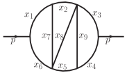
(b)

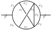
(c)

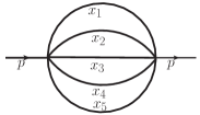
(d)

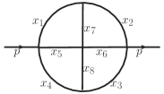
Figure 8: 4-loop self-energy diagrams with massless internal lines, cf., Baikov and Chetyrkin [2]: (a) $N=9$, (b) $N=9$, (c) $N=5$, (d) $N=8$

Table 23: ParInt accuracy and times (on 4 nodes/64 procs. thor cluster) for the loop integrals of the diagrams of Fig 8(a) and (b) ($M_{44}$ and $M_{45}$ in Baikov and Chetyrkin [2]) with $\varrho=\varepsilon=0,$ using various numbers of function evaluations.

Diagram	# Fcn.	Integral	Rel. err.	Time
	Evals.	Result	Est. $E_{r}$	T[s]
Fig 8 (a)	100B	55.594725	9.87e-04	185.1
	200B	55.586822	3.53e-04	370.0
	300B	55.585150	1.80e-04	554.3
	Eq (48):	55.585254
Fig 8 (b)	100B	52.026428	9.84e-04	239.5
	200B	52.019118	3.63e-04	479.9
	275B	52.017714	2.20e-04	658.8
	Eq (49):	52.017869

6.2 4-loop UV-divergent integrals

This section handles the integrals associated with the massless diagrams of Fig 8(c) and (d) (the 4-loop sunrise-sunset and Shimadzu diagrams named $M_{01}$ and $M_{36},$ respectively, in [2]), which have a UV singularity from the $\Gamma$-function factor in Eq (45). We put $\varrho=0$ in the integrals for Fig 8 (c) and (d), and consider the expansions in $\varepsilon.$

For the integral $I_{c}^{S4}$ in Fig 8, the $U,\,W$ functions are

$$\mathrm{(c)}\quad\left\{\begin{array}[]{l}U=x_{1}x_{2}x_{3}x_{4}+x_{1}x_{2}x_{3}x_{5}+x_{1}x_{2}x_{4}x_{5}+x_{1}x_{3}x_{4}x_{5}+x_{2}x_{3}x_{4}x_{5}\\ W/s=x_{1}x_{2}x_{3}x_{4}x_{5}\end{array}\right.\,.$$ (50)

The numerical results are compared with the expansion in Baikov and Chetyrkin [2],

$$n(\varepsilon)^{4}I_{c}^{S4}=-\frac{1}{576}\,\frac{1}{\varepsilon}-\frac{13}{768}-\frac{9823}{82944}\,\varepsilon+\,\ldots$$

$$=-0.001736111111\,\frac{1}{\varepsilon}-0.016927083333-0.118429301698\,\varepsilon+\,\ldots$$ (51)

Note that $I=I_{c}^{S4}$ of Eq (45) is multiplied with $n(\varepsilon)^{4},$ where $n(\varepsilon)$ is defined in Eq (35).

Based on integrations with ParInt, using a maximum of 10B function evaluations and an absolute error tolerance of $10^{-12}$ (on the computation of the integral $I_{c}^{S4}/\Gamma(-3+4\varepsilon)$), the results in Table 24 are produced using linear extrapolation. ParInt returns a 0 error flag for the integrals constituting the input sequence to the extrapolation, indicating that a successful termination is assumed according to Eqs (2) or (14) for the requested accuracy.

Table 24: Results UV 4-loop sunrise-sunset integral, Fig 8 (c) (on 4 nodes/64 procs. thor cluster), err. tol. $t_{a}=10^{-12},$ $T[s]$ = Time (elapsed user time in seconds); $\varepsilon=\varepsilon_{\ell}=2^{-\ell},\leavevmode\nobreak\ \ell=8,9,\ldots,$   $E_{a}=$ integration estim. abs. error

	Integral $I_{c}^{S4}$		Extrapolation
$\ell$	$E_{a}$	T[s]	Result  ${C}_{-1}$	Result  ${C}_{0}$	Result  ${C}_{1}$
$8$	3.9e-14	30.2
$9$	3.8e-14	34.3	-0.001735179254977
$10$	3.6e-14	34.1	-0.001736115881839	-0.016918557081	-0.012276556
$11$	4.1e-14	50.8	-0.001736111099910	-0.016927126297	-0.011837812
$12$	4.2e-14	58.5	-0.001736111111130	-0.016927083216	-0.011842959
$13$	1.5e-14	48.1	-0.001736111111109	-0.016927083381	-0.011842916
Eq (51):			-0.001736111111111	-0.016927083333	-0.011842930

For $I_{d}^{S4}$ of the $N=8$ diagram shown in Fig 8 (d) (Shimadzu, named $M_{36}$ in [2, 13]), the $U,W$ functions are:

$$\mathrm{(d)}\quad\left\{\begin{array}[]{l}U=x_{7}x_{8}\,(x_{12}x_{3456}+x_{34}x_{56})+x_{78}x_{1234}x_{5}x_{6}\\ \quad+x_{7}\,(x_{5}x_{3}x_{124}+x_{6}x_{4}x_{123}+x_{3}x_{4}x_{12})+x_{8}\,(x_{5}x_{2}x_{134}+x_{6}x_{1}x_{234}+x_{1}x_{2}x_{34})\\ \quad+x_{5}x_{6}x_{14}x_{23}+x_{5}x_{2}x_{3}x_{14}+x_{6}x_{1}x_{4}x_{23}+x_{1}x_{2}x_{3}x_{4}\\ W/s=x_{7}x_{8}x_{12}x_{34}x_{56}+x_{78}x_{12}x_{34}x_{5}x_{6}+x_{7}x_{12}x_{3}x_{4}x_{56}+x_{8}x_{1}x_{2}x_{34}x_{56}\\ \quad+x_{5}x_{6}\,(x_{1}x_{2}x_{34}+x_{12}x_{3}x_{4})+x_{56}x_{1}x_{2}x_{3}x_{4}\end{array}\right.$$ (52)

The expansion given in [2] is

$$n(\varepsilon)^{4}I_{d}^{S4}=\frac{5\zeta_{5}}{\varepsilon}-5\zeta_{5}-7\zeta_{3}^{2}+\frac{25}{2}\zeta_{6}+\,(35\zeta_{5}+7\zeta_{3}^{2}-\frac{25}{2}\zeta_{6}-21\zeta_{3}\zeta_{4}+\frac{127}{2}\zeta_{7})\,\varepsilon+\,\ldots,$$

$$=\frac{5.184638776}{\varepsilon}-2.582436090+70.39915145\,\varepsilon+\,\ldots$$ (53)

This is $I=I_{d}^{S4}$ of Eq (45) multiplied with $n(\varepsilon)^{4},$ where $n(\varepsilon)$ is defined in Eq (35). The numerical result by FIESTA is shown in [13] and it is $5.184645\pm 0.000042$.

The results by the DE formula (15) with $N_{eval}=49$ and mesh size $h=0.125$ in all dimensions, and linear extrapolation, are shown in Table 25. The starting $\varepsilon$ is $2^{-10}.$ The time required for each iteration using 64 threads on KEKSC System A, SR16000 Model M1 (POWER7(R) processor) is below 20 minutes.

Table 25: Results UV 4-loop Shimadzu integral, $I_{d}^{S4}$, Fig 8 (d), (on KEKSC 64 threads); $\varepsilon=\varepsilon_{\ell}=2^{-\ell},\leavevmode\nobreak\ \ell=10,11,\ldots,$.

Integral $I_{d}^{S4}$	Extrapolation
$\ell$	Result  ${C}_{-1}$	Result  ${C}_{0}$	Result  ${C}_{1}$
$10$
$11$	5.18460577	-2.47956688
$12$	5.18463921	-2.58230627	70.1367604
$13$	5.18463922	-2.58243393	70.3982056
$14$	5.18463923	-2.58243413	70.3991764
Eq  (53):	5.18463878	-2.58243609	70.3991515

7 Conclusions

In this paper we describe a fully numerical method for Feynman loop integrals, based on numerical multi-dimensional integration and linear or non-linear extrapolation. We use three categories of numerical integration methods, iterated integration with Dqage (Dqags) from Quadpack, multivariate adaptive integration with ParInt, and the DE formula. For the numerical extrapolation, we employ nonlinear extrapolation with geometric sequences of the extrapolation parameter, and linear extrapolation with Bulirsch or geometric sequences. The main advantage of the method is its general applicability to multi-loop integrals with arbitrary physical masses and external momenta, without resorting to special problem formulations. Using dimensional regularization, both UV-divergent and finite terms are estimated. We have shown that the technique works well for sets of diagrams with up to four loops and up to four external lines, with or without UV-divergence, and the numerical results reveal excellent agreement with expansions in the literature [1, 2, 13].

We also demonstrate the effectiveness of variable transformations for some integrals. Regardless of whether or not variables are transformed, the formulation of the numerical method is not affected and it is only necessary to replace the integrand and Jacobian. The way to transform variables for a loop integral is not unique, and a general technique to find the most effective transformation is not currently known. However, the effectiveness of transformations can be assessed by examining the behavior of the integrations and the ensuing convergence of the extrapolation. The experience gained with the transformations in this paper will yield guidelines to construct a more general procedure, which will be studied in future work.

The computation time of the numerical multivariate integration increases with the number of internal lines, i.e., with the dimension of integration. For example, though we understand the importance of scattering processes with more external legs than five or six in two-loop order, this is beyond the scope of the current paper, and we plan on addressing these and related types of problems in future work.

Furthermore, while the examples shown here are limited to scalar loop integrals, they can easily be extended to more general cases with physical masses and external momenta, by including the associated numerator in the integrand (see [4]). The present work includes integrals with massive and massless internal particles. For massive particles, a mass value of one is assigned in order to compare results with the literature [1]. Massless cases are compared, e.g., with results in [2]. In view of the numerical nature of the methods there is in principle no limitation for the general mass values, even though challenges may arise with respect to computing time vs. computational precision. We are helped in dealing with this trade-off by the evolution in computer architecture and the computational techniques.

Appendix A Analytic method for Fig 2(d)(c)

This Appendix derives the analytic result for the 2-loop half-boiled egg diagram of Fig 2(d)(c).

By the variable transformation

$x_{1}=\tau\,(1-\xi)$,  $x_{2}=\tau\,\xi$,  $x_{3}=(1-\tau)\,\tau^{\prime}\,(1-\xi^{\prime})$,  $x_{4}=(1-\tau)\,\tau^{\prime}\,\xi^{\prime}$,  $x_{5}=(1-\tau)\,(1-\tau^{\prime}),$

the functions $U,V$ are given by

$$U=\tau\,F,\quad F=1-\tau+\tau\,\xi\,(1-\xi)$$

$$W/s=\tau\,G,\quad G=(1-\tau)\,(1-\tau^{\prime})\,((1-\tau)\,\tau^{\prime}+\tau\,\xi\,(1-\xi))$$

and

$$J_{c}^{S2}=\int_{0}^{1}d\tau\leavevmode\nobreak\ \tau(1-\tau)^{2}\int_{0}^{1}d\xi\int_{0}^{1}d\tau^{\prime}\,\tau^{\prime}\frac{1}{U^{1-3\varepsilon}\,(UV)^{1+2\varepsilon}}$$ (54)

where we assume $m_{3}=m_{4}$ to perform the $\xi^{\prime}$-integration.

The integral is divergent at $\tau=0$ to produce $\displaystyle{1/\varepsilon}$ singularity, and the separation of the singularity is done as follows. Let us denote $H=M^{2}F-s\,G,$ and let us use the suffix 0 for the function defined at $\tau=0$, i.e., $F_{0}=F\,(\tau=0)=1$ and $H_{0}=H\,(\tau=0)=[\tau^{\prime}m_{3}^{2}+(1-\tau^{\prime})\,m_{5}^{2}]-s\,(1-\tau^{\prime})\,\tau^{\prime}$.

The integral is separated into two terms as

$$J_{c}^{S2}=I_{A}+I_{B}$$

where the first term $I_{A}$ has a UV singularity. The integrands of $I_{A}$ and $I_{B}$ are given according to Eq (54) and

$$\frac{1}{U^{1-3\varepsilon}(UV)^{1+2\varepsilon}}=\frac{1}{\tau^{2-\varepsilon}}\frac{1}{F^{1-3\varepsilon}H^{1+2\varepsilon}}=\frac{1}{\tau^{2-\varepsilon}}\left[\frac{1}{F_{0}^{1-3\varepsilon}H_{0}^{1+2\varepsilon}}+\left(\frac{1}{F^{1-3\varepsilon}H^{1+2\varepsilon}}-\frac{1}{F_{0}^{1-3\varepsilon}H_{0}^{1+2\varepsilon}}\right)\right]\,.$$

The divergent term $I_{A}$ is trivial in the $\xi$-integral and is calculated as

$$I_{A}=\int_{0}^{1}d\tau\,\frac{(1-\tau)^{2}}{\tau^{1-\varepsilon}}\int_{0}^{1}d\tau^{\prime}\frac{\tau^{\prime}}{H_{0}^{1+2\varepsilon}}$$

$$=\left(\frac{1}{\varepsilon}-\frac{3}{2}+\frac{7}{4}\varepsilon-\frac{15}{8}\varepsilon^{2}\right)\times\left(I_{A}^{(0)}+I_{A}^{(1)}\varepsilon+I_{A}^{(2)}\varepsilon^{2}+I_{A}^{(3)}\varepsilon^{3}\right)$$ (55)

and the non-divergent term $I_{B}$ is

$$I_{B}=\int_{0}^{1}d\tau\int_{0}^{1}d\xi\int_{0}^{1}d\tau^{\prime}\,\frac{(1-\tau)^{2}\tau^{\prime}}{\tau^{1-\varepsilon}}\left(\frac{1}{F^{1-3\varepsilon}H^{1+2\varepsilon}}-\frac{1}{H_{0}^{1+2\varepsilon}}\right)$$

$$=I_{B}^{(1)}+I_{B}^{(2)}\varepsilon+I_{B}^{(3)}\varepsilon^{2}$$ (56)

The terms $I_{A}^{(0)},I_{A}^{(1)},I_{A}^{(2)},I_{A}^{(3)}$ and $I_{B}^{(1)},I_{B}^{(2)},I_{B}^{(3)}$ in Eqs (55) and (56) can be obtained by expanding the integrands in powers of $\varepsilon$. We evaluated these terms numerically by Dqage and Dqags from Quadpack and the DE formula, for the values $s=M^{2}=1,$ yielding the expression in Eq (20).

References

References

- [1] Laporta S 2000 Int. J. Mod. Phys. A 15 5087–5159 arXiv:hep-ph/0102033v1
- [2] Baikov B A and Chetyrkin K G 2010 Nuclear Physics B 837 186–220
- [3] de Doncker E, Shimizu Y, Fujimoto J and Yuasa F 2004 Computer Physics Communications 159 145–156
- [4] de Doncker E, Shimizu Y, Fujimoto J, Yuasa F, Cucos L and Van Voorst J 2004 Nuclear Instruments and Methods in Physics Research A 539 269–273 hep-ph/0405098
- [5] Yuasa F, de Doncker E, Fujimoto J, Hamaguchi N, Ishikawa T and Shimizu Y 2007 Precise numerical results of IR-vertex and box integration with extrapolation XI Adv. Comp. and Anal. Tech. in Phys. Res. PoS (ACAT07) 087, arXiv:0709.0777v2 [hep-ph]
- [6] Yuasa F, Ishikawa T, Fujimoto J, Hamaguchi N, de Doncker E and Shimizu Y 2008 Numerical evaluation of Feynman integrals by a direct computation method XII Adv. Comp. and Anal. Tech. in Phys. Res. PoS (ACAT08) 122; arXiv:0904.2823
- [7] de Doncker E, Fujimoto J, Kurihara Y, Hamaguchi N, Ishikawa T, Shimizu Y and Yuasa F 2010 Recursive box and vertex integrations for the one-loop hexagon reduction in the physical region XIII Adv. Comp. and Anal. Tech. in Phys. Res. PoS (ACAT10) 073
- [8] Yuasa F, de Doncker E, Hamaguchi N, Ishikawa T, Kato K, Kurihara Y and Shimizu Y 2012 Journal Computer Physics Communications 183 2136–2144
- [9] de Doncker E, Fujimoto J, Hamaguchi N, Ishikawa T, Kurihara Y, Shimizu Y and Yuasa F 2011 Journal of Computational Science (JoCS) 3 102–112 doi:10.1016/j.jocs.2011.06.003
- [10] de Doncker E, Li S, Fujimoto J, Shimizu Y and Yuasa F 2005 Springer Lecture Notes in Computer Science (LNCS) 3514 165–171
- [11] de Doncker E, Fujimoto J, Hamaguchi N, Ishikawa T, Kurihara Y, Ljucovic M, Shimizu Y and Yuasa F 2010 Extrapolation algorithms for infrared divergent integrals arXiv:hep-ph/1110.3587; PoS (CPP2010)011
- [12] de Doncker E, Yuasa F and Kurihara Y 2012 Journal of Physics: Conf. Ser. 368
- [13] Smirnov A V and Tentyukov M 2010 Nuclear Physics B 837 40–49
- [14] de Boor C 1971 CADRE: An algorithm for numerical quadrature Mathematical Software ed Rice J R (Academic Press, New York) pp 417–449
- [15] Piessens R, de Doncker E, Überhuber C W and Kahaner D K 1983 QUADPACK, A Subroutine Package for Automatic Integration (Springer Series in Computational Mathematics vol 1) (Springer-Verlag)
- [16] de Doncker E and Yuasa F 2013 Journal of Physics: Conf. Series 410 012047 doi:10.1088/1742-6596/410/1/012047
- [17] de Doncker E, Yuasa F and Assaf R 2013 Journal of Physics: Conf. Ser. 454 doi:10.1088/1742-6596/454/1/012082
- [18] de Doncker E and Yuasa F 2014 XV Adv. Comp. and Anal. Tech. in Phys. Res., Journal of Physics: Conference Series (ACAT 2013) 523 doi:10.1088/1742-6596/523/1/012052
- [19] Shanks D 1955 J. Math. and Phys. 34 1–42
- [20] Wynn P 1956 Mathematical Tables and Aids to Computing 10 91–96
- [21] Sidi A 1996 Journal of Approximation Theory 86 21–40
- [22] Sidi A 2003 Practical Extrapolation Methods - Theory and Applications (Cambridge University Press) iSBN 0-521-66159-5
- [23] Sidi A 2011 Numer. Math. 119 725–764
- [24] OpenMP http://www.openmp.org
- [25] Takahasi H and Mori M 1974 Publications of the Research Institute for Mathematical Sciences 9 721–741
- [26] Davis P J and Rabinowitz P 1984 Methods of Numerical Integration (Academic Press, New York)
- [27] Sugihara M 1997 Numerische Mathematik 75 379–395
- [28] Brezinski C 1980 Numerische Mathematik 35 175–187
- [29] Bulirsch R 1964 Numerische Mathematik 6 6–16
- [30] Lyness J N 1976 Journal of Computational Physics 20 346–364
- [31] Fritsch F N, Kahaner D K and Lyness J N 1981 ACM TOMS 7 46–75
- [32] Kahaner D, Moler C and Nash S 1988 Numerical Methods and Software (Prentice Hall)
- [33] de Doncker E and Kaugars K 2010 Procedia Computer Science 1 117–124
- [34] Open-MPI http://www.open-mpi.org
- [35] de Doncker E, Yuasa F, Kapenga J and Olagbemi O 2015 The Journal of Physics: Conf. Series (JPCS) 640 doi:10.1088/1742-6596/640/1/012062
- [36] Genz A and Malik A 1980 Journal of Computational and Applied Mathematics 6 295–302
- [37] Genz A and Malik A 1983 SIAM J. Numer. Anal. 20 580–588
- [38] Berntsen J, Espelid T O and Genz A 1991 ACM Trans. Math. Softw. 17 437–451
- [39] Genz A 1990 An adaptive numerical integration algorithm for simplices Lecture Notes in Computer Science vol 507 ed Sherwani N A, de Doncker E and Kapenga J A pp 279–285
- [40] Grundmann A and Möller H 1978 SIAM J. Numer. Anal. 15 282–290
- [41] de Doncker E 1979 Math. Comp. 33 1003–1018
- [42] Berntsen J, Espelid T O and Genz A 1991 ACM Trans. Math. Softw. 17 452–456 http: //www.sci.wsu.edu/math/faculty/genz/homepage
- [43] de Doncker E, Gupta A and Ealy P 1996 Lecture Notes in Computer Science, Springer-Verlag 1067 562–570
- [44] de Doncker E, Kaugars K, Cucos L and Zanny R 2001 Current status of the ParInt package for parallel multivariate integration Proc. of Computational Particle Physics Symposium (CPP 2001) pp 110–119
- [45] Achalla C, Kaugars K and de Doncker E 2003 Load balancing in distributed adaptive task partitioning Parallel and Distributed Computing and Systems pp 280–283
- [46] Achalla C, de Doncker E, Kaugars K and VanṼoorst J 2004 -load balancing for parallel adaptive task partitioning Parallel and Distributed Computing and Systems
- [47] ParInt http://www.cs.wmich.edu/parint
- [48] Motoki S, Daisaka H, Nakasato N, Ishikawa T, Yuasa F, Fukushige T, Kawai A and Makino J 2015 The Journal of Physics: Conf. Series (JPCS) 608 doi:10.1088/1742-6596/608/1/012011
- [49] de Doncker E, Yuasa F and Olagbemi F 2015 Procedia Computer Science 51 1333–1342 doi:10.1016/j.procs.2015.05.318
- [50] de Doncker E, Yuasa F, Kato K, Ishikawa T and Olagbemi O 2015 The Journal of Physics: Conf. Series (JPCS) 608 doi:10.1088/1742-6596/608/1/012071
- [51] de Doncker E, Yuasa F, Kato K and Ishikawa T 2016 Automatic numerical integration and extrapolation for Feynman loop integrals Workshop on Computational Particle Physics (CPP2016) Under review