Visualization of the global flow structure in a modified Rayleigh-Bénard setup using contactless inductive flow tomography

Abstract

Rayleigh-Bénard convection is not only a classical problem in fluid dynamics but plays also an important role in many metallurgical and crystal growth applications. The measurement of the flow field and of the dynamics of the emerging large-scale circulation in liquid metals is a challenging task due to the opaqueness and the high temperature of the melts. Contactless inductive flow tomography is a technique to visualize the mean three-dimensional flow structure in liquid metals by measuring the flow induced magnetic field perturbations under the influence of one or several applied magnetic fields. In this paper, we present first measurements of the flow induced magnetic field in a Rayleigh-Bénard setup, which are also used to investigate the dynamics of the large-scale circulation. Additionally, we investigate numerically the quality of the reconstruction of the three-dimensional flow field for different sensor configurations.

1 Introduction

Buoyancy driven flows of fluids heated from below and cooled from above play a key role in geo- and astrophysics, in the natural ventilation of buildings, and in many metallurgical applications. It is thus no surprise that Rayleigh-Bénard (RB) convection has served as one of the central paradigms for stability theory, pattern formation, and scaling behavior [1].

Besides asking how global thermohydraulic features such as the Reynolds and the Nusselt number depend on the Rayleigh and the Prandtl number [2], special focus of RB studies has been laid on the phenomenon of large-scale convection (LSC) [3, 4, 5, 6, 7, 8, 9, 10]. LSC appears at sufficiently high values of the Rayleigh number, when thermal plumes erupt from the boundary layers and self-organize into a flywheel structure [1]. The dynamics of this global wind has turned out surprisingly rich, comprising torsional modes [11] and sloshing modes [12, 13], as well as global reorientations by azimuthal rotations and (rare) cessations [8, 10]. A number of experiments dedicated to these LSC problems were carried out with water [3, 8, 10], silicon oil [3], helium-gas [4], air [9], and liquid mercury [5, 6].

RB experiments with liquid metals are not only fundamentally important to explore the low Prandtl number regime, but are also relevant for a variety of metallurgical and crystal growth applications. For instance, in the Czochralski (Cz) crystal growth of mono-crystalline silicon large temperature gradients are inherently present at the crystallization edge which lead to strong temperature fluctuations [14, 15]. The control (and optimization) of these fluctuations still remains a challenge. The flow structure, which plays a key role for the quality of the final crystal since it controls the temperature gradient and mass transport, is governed by the details of heating and the differential rotation of crucible and crystal. For stabilizing the flow, external magnetic fields are frequently used [14].

While dedicated RB experiments with low-melting liquid metals such as mercury and GaInSn can easily be equipped with direct contact sensors such as thermistors [6] or ultrasonic transducers [16], industrial high temperature applications (e.g. with liquid silicon) demand for contactless flow measurement techniques.

A step in this direction is the contactless inductive flow tomography (CIFT) [17, 18, 19], which is able to provide a picture of the three-dimensional flow by applying primary magnetic fields to the melt and by measuring the flow induced magnetic field perturbation outside the fluid volume. From these field perturbations CIFT infers the flow field by solving a linear inverse problem. Appropriate regularization techniques, like Tikhonov regularization in combination with the L-curve technique [20], are necessary in order to mitigate the intrinsic non-uniqueness of the inverse problem. In a first demonstration experiment [18], the propeller stirred three-dimensional flow of the eutectic alloy GaInSn in a cylindrical vessel was reconstructed. The CIFT-inferred mean velocity turned out to be in good agreement with comparative ultrasonic Doppler flow measurements. Later, CIFT was successfully applied to visualize the (essentially two-dimensional) flow field in the mold of a laboratory model of continuous slab casting [21, 22, 23].

As for Czochralski crystal growth, any real application of CIFT to determine the flow in a Cz-puller would face a number of problems. Due to the high temperature of about 1500^∘ C in the oven, the magnetic field sensors can only be placed outside the device, which necessarily results in a large distance between the sensors and the melt. To make matters worse, the typical meridional flow velocity is only in the order of a few cm/s, i.e. one order of magnitude smaller than in the case of continuous casting. Both facts would decrease significantly the ratio between the measurable induced field and the applied magnetic field, which is a crucial criterion for the technical applicability of CIFT.

Motivated by this challenge, this paper is intended to examine the viability of CIFT for measuring liquid metal velocities in the order of 1 cm/s as they are typical for liquid metal RB convection in general, and for Czochralski crystal growth in particular. For this purpose, an existing set-up of a modified RB convection cell [15] has been equipped with one pair of excitation coils, generating a basically vertical magnetic field in the fluid, and 20 magnetic field sensors which are situated along the azimuth, approximately at mid-height of the convection cell (Fig. 1).

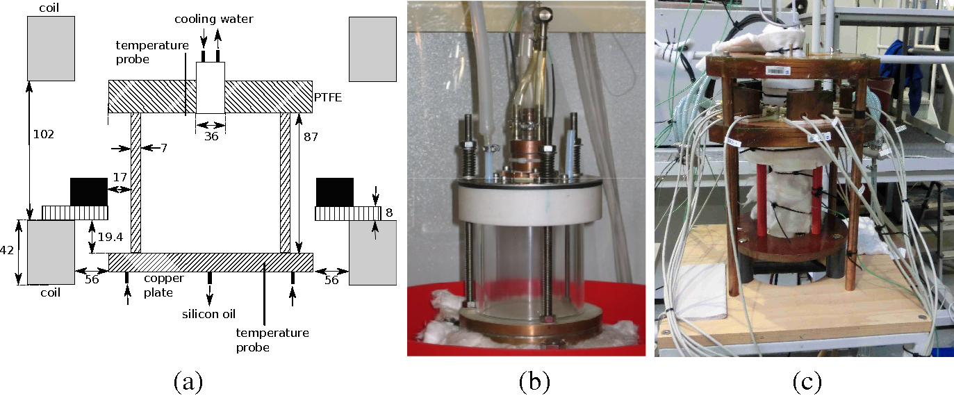
Figure 1: Schematic sketch (a), photography of the cell (b), and photography of the complete set-up (c) of the RB experiment.

We will demonstrate that typical dynamical features of the LSC, like azimuthal rotations and even cessations, as well as the typical frequencies of the torsional/sloshing mode [13] are well detectable. While our main goal is to proof the principle applicability of CIFT for RB flows, a full three-dimensional flow reconstruction would require more sensors at different heights, and, perhaps, a second magnetic field to be applied in horizontal direction. Therefore, we will also examine numerically the quality of the CIFT-reconstructed velocity field for such enhanced measurement configurations.

The paper is structured as follows: after a short reminder of the basic principles and some numerical tests of CIFT for a typical LSC structure, we will describe the experimental setup and present investigations of the dynamics of the azimuthal orientation of LSC for five specific temperature differences. Based on those measurements, we will discuss some preliminary results of the CIFT-reconstruction with our reduced sensor configuration.

2 Contactless inductive flow tomography and RB flows

In this section we discuss the mathematical basics of CIFT and examine numerically how it can be applied to typical RB convection problems.

2.1 Basics of CIFT

Here, we only briefly delineate the theory of CIFT. More details, in particular concerning the non-uniqueness problem of the ill-posed inverse problem, and how to mitigate it, can be found in previous papers [17, 24].

Assume an electrically conductive fluid with a velocity field $\bf v$ exposed to a magnetic field $\bf B$. According to Ohm’s law in moving conductors, a current density

$${\bf j} = \sigma({\bf v}\times{\bf B}-\nabla\varphi)$$ (1)

will be induced, with $\sigma$ denoting the electrical conductivity of the fluid and $\varphi$ the electric scalar potential. Applying Biot-Savart’s law [17], this current density ${\bf j}$ induces the following (secondary) magnetic field ${\bf b}({\bf r})$:

$${\bf b}({\bf r}) = \frac{\mu_{0}\sigma}{4\pi}\iiint\limits_{V}[{\bf v}({\bf r}^{\prime})\times{\bf B}({\bf r}^{\prime})]\times\frac{{\bf r}-{\bf r}^{\prime}}{|{\bf r}-{\bf r}^{\prime}|^{3}}dV^{\prime}$$ (2)

$$-\frac{\mu_{0}\sigma}{4\pi}\oiint\limits_{S}\varphi({\bf s}^{\prime}){\bf n}({\bf s}^{\prime})\times\frac{({\bf r}-{\bf s}^{\prime})}{|{\bf r}-{\bf s}^{\prime}|^{3}}dS^{\prime}\;.$$

It is important to incorporate the surface integral on the r.h.s. of Eq. (2) which, in certain circumstances, can completely cancel the volume integral term (early attempts [25, 26] to develop a CIFT-like magnetic flow tomography were flawed by this omission).

Exploiting the divergence-free condition of $\bf j$, Eq. (1) leads to a Poisson equation for the electric potential:

$$\Delta\varphi = \nabla\cdot({\bf v}\times{\bf B})\;.$$ (3)

Using Green’s theorem, the solution of this Poisson equation can be shown to fulfill the boundary integral equation

$$\varphi({\bf s}) = \frac{1}{2\pi}\iiint\limits_{V}[{\bf v}({\bf r}^{\prime})\times{\bf B}({\bf r}^{\prime})]\cdot\frac{{\bf s}-{\bf r}^{\prime}}{|{\bf s}-{\bf r}^{\prime}|^{3}}dV^{\prime}$$ (4)

$$-\frac{1}{2\pi}\oiint\limits_{S}\varphi({\bf s}^{\prime}){\bf n}({\bf s}^{\prime})\cdot\frac{({\bf s}-{\bf s}^{\prime})}{|{\bf s}-{\bf s}^{\prime}|^{3}}dS^{\prime}\;,$$

if insulating boundaries are assumed.

In general, the total magnetic field $\bf B$ under the integrals of Eqs. (2) and (4) is the sum of an externally applied (primary) magnetic field ${\bf B}_{0}$ and the induced (secondary) magnetic field $\bf b$ itself. The ratio between $\bf b$ and ${\bf B}_{0}$ is proportional to the magnetic Reynolds number $Rm$ of the flow, defined as

$$Rm=\mu_{0}\sigma lv\;,$$ (5)

with $l$ and $v$ denoting characteristic length and velocity scales of the fluid, respectively. For large values of $Rm$, and appropriate flow topologies, it is possible to achieve self-excitation of a magnetic field. In this case, one can obtain solutions of Eqs. (2) and (4) even for ${\bf B}_{0}=0$ , an effect that is known as homogeneous dynamo action [27, 28].

However, in most industrial applications, and in particular in typical RB convection problems, $Rm$ is typically smaller than $1$. As for the experiment to be discussed here, with a vessel width of approximately 0.1 m, a typical LSC velocity of $v_{LSC}\approx 1$ cm/s, and a conductivity of the liquid GaInSn of $3.27\times 10^{6}$ S/m, we obtain $Rm\approx 0.004$. In such cases, it is well justified to replace ${\bf B}$ by ${\bf B}_{0}$ under the integrals in Eqs. (2) and (4). Thereby, we arrive at a linear inverse problem for the determination of the velocity field $\bf v$ from the induced magnetic field $\bf b$ that is supposed to be measured in the exterior of the fluid. Note that the primary magnetic field can be applied in various directions. As long as the typical time for velocity changes is larger than the switching times for the different applied fields, this allows to collect more information about (basically) the same velocity field which can further mitigate the non-uniqueness of the inverse problem. Examples of its solution in cylindrical geometry, and details on how to apply the Tikhonov regularization, can be found in [18, 29].

2.2 Numerical tests of CIFT for RB flows

In the following, we will discuss how CIFT can be employed to infer the typical LSC flow structure of RB convection. For this purpose we have first simulated the RB flow using the buoyantBoussinesqPimpleFoam solver of the finite volume library OpenFOAM. No turbulence models were used. The time-average of the resulting flow served then as the basis for computing the induced magnetic fields according to Eqs. (2) and (4). Finally, these fields were used, in turn, as input for reconstructing the velocity structure by solving the linear inverse problem. In this step, we tested various (hypothetical) configurations of magnetic field sensors situated around the vessel, and applied also different combinations of primary magnetic fields.

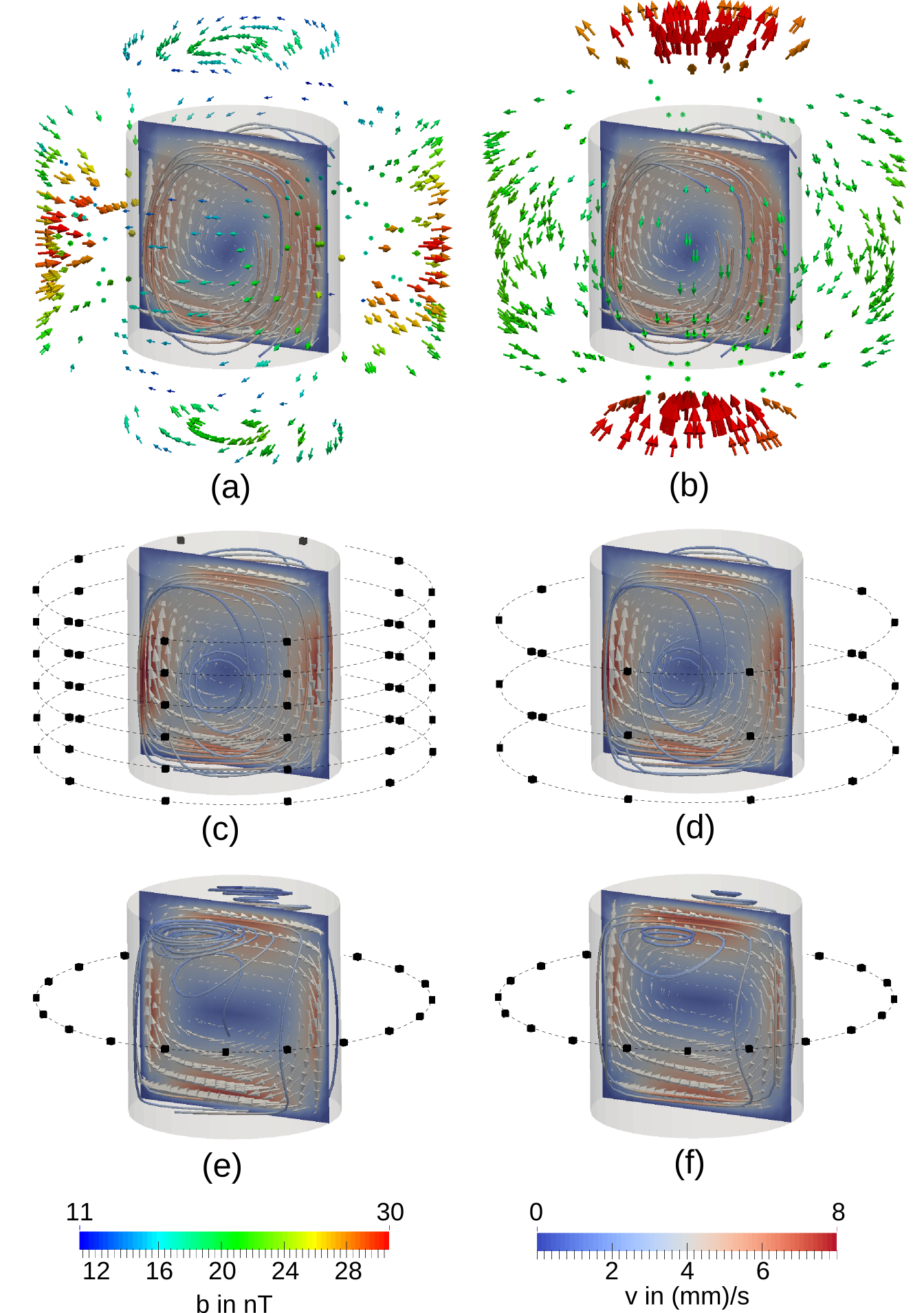
Figure 2: Numerical tests of CIFT for an RB flow at $\Delta T=2.2$ K. (a) OpenFOAM-simulated velocity structure, and the induced magnetic field for an applied vertical field. (b) As in (a), but for an applied horizontal field. (c) Measurement configuration with 6$\times$10 sensors, and CIFT inferred velocity for applying both a vertical and a horizontal field. (d) As in (c), but for 3$\times$10 sensors. (e) As in (c), but for 1$\times$20 sensors. (f) As in (e), but restricted to measurements with only applied vertical field.

Figs. 2a,b show the OpenFOAM-simulated, time-averaged velocity field for a temperature difference of $2.3$ K, together with the flow-induced magnetic field for applied vertical field (a) and applied horizontal field (b), and the CIFT-reconstructed velocity field by assuming four different measuring configurations (c,d,e,f). For the inversion shown in Fig. 3c we assume homogeneous vertical and horizontal primary fields of $3$ mT to be applied, and a hypothetical number of 6$\times$10 sensors distributed over 6 heights and 10 azimuths around the mantle of the cylinder. The visual impression of an excellent coincidence between the original (Fig. 2a) and the reconstructed flow (Fig. 2c) is supported by an empirical correlation coefficient as high as 0.95 and a relative rms error as low as 0.09. A similar coincidence holds if the number of sensors is reduced to $3\times 10$ as in Fig. 2d. Then the inversion ends up with an empirical correlation coefficient of 0.95 and a relative rms error of 0.11.

Amazingly, even the strongly reduced sensor configuration as used in our experiment, with 20 sensors at mid-height, distributed regularly along the azimuth, provides reasonable results. When applying both a vertical and a horizontal field (Fig. 2e) we still obtain an empirical correlation coefficient of 0.84 and a relative rms error of 0.29. The minor deterioration of the agreement seems to be connected with the appearance of an (artificial) eddy structure at the top, where some necessary magnetic field information is obviously missing. Even when restricting the measurements to the case of a vertically applied field (Fig. 2f), we still get a reasonable empirical correlation coefficient of 0.8 and a relative rms error of 0.36. This surprisingly robust behavior of CIFT suggests to start our RB investigation with the reduced measurement configuration as shown in Fig. 2f.

3 Experimental setup

The setup of our RB experiment (Fig. 1) consists of a cylindrical column filled with the eutectic liquid alloy GaInSn that is homogeneously heated from below. In trying to emulate the growing crystal of a Czochralski system, only partial cooling of the top is realized by means of a circular heat exchanger mounted concentrically within the upper lid. This partial cooling covers approximately the same relative area as the growing crystal in a real Cz-puller. Both heat exchangers (heater and cooler) are made of copper with branched channels to minimize any remaining temperature gradients. PID-controlled thermostats with a large reservoir were used to supply both the top heat exchanger and the bottom plate with the coolant/heating fluid at high flow rate. Fig. 1b shows a photograph of the experimental cell with the diameter and height of $D=H=87$ mm (aspect ratio $\Gamma=D/H=1$). The transparent side wall is made of borosilicate glass, because of its low heat conductivity. During the measurements, the whole apparatus is embedded in mineral wool in order to minimize lateral heat loss (Fig. 1c).

For a given temperature difference $\Delta T$ between bottom and top, we obtain an (approximate) Rayleigh number of

$$Ra = \frac{g\beta}{\kappa\nu}H^{3}\Delta T$$ (6)

$$= \frac{g\beta\rho c_{p}}{\lambda\nu}H^{3}\Delta T$$

$$= 3.42\times 10^{8}\frac{H^{3}\Delta T}{m^{3}K}$$

$$= 2.25\times 10^{5}\frac{\Delta T}{K}$$

by considering $g=9.81$ m/s² and the following material parameters of GaInSn at $20^{\circ}$ C [30]: thermal expansion coefficient $\beta=1.24\times 10^{-4}$ K^-1, density $\rho=6350$ kg/m³, specific heat capacity at constant pressure $c_{p}=366$ J/(kg k), viscosity $\nu=3.44\times 10^{-7}$ m²/s, thermal diffusivity $\lambda=24.0$ W/(m K). Note that, in particular at high $\Delta T$, $Ra$ should be determined more accurately by taking into account the temperature dependence of material parameters (which here are simply fixed to a reference temperature of 20^∘ C). Note also that, even for the same value of $Ra$, one should not expect a perfect agreement with other liquid metal RB experiments, because of the partial cooling at the top.

In the first experimental realization of CIFT, the excitation magnetic field is generated by only one pair of circular coils which are fed by a current of 20 A generating in the fluid a fairly homogeneous vertical field $B_{z}$ of approximately 4 mT. In asking whether this field itself could have an influence on the flow structure, we determine the Hartmann number as $Ha=B_{z}H(\sigma/(\rho\nu)^{1/2}\approx 13$, and the maximum expectable interaction parameter (estimated for the lowest LSC velocity of $v_{LSC}\approx 0.5$ cm/s) as $N=Ha^{2}/Re\approx 0.14$. Both values suggest that the influence of the measuring field on the flow should be minor.

The coils are cooled in order to minimize temperature changes over time. In contrast to the more advanced measurement configurations as numerically examined in the previous section, the flow induced magnetic field is measured by only 20 Fluxgate probes which are regularly distributed over the azimuth, approximately at mid-height of the RB vessel. The measured magnetic field component is always the radial one, pointing normally to the nearest surface point of the vessel. For low $\Delta T$, the measured induced magnetic field is typically in the order of $10...100$ nT, which is a factor 10^-5 smaller than the primary magnetic field! For this reason it is essential to guarantee a very stiff mounting of the sensors with respect to the coils in order to minimize bias magnetic field perturbations that would result from any deformations due to thermal expansion of the coil and/or the sensor holders.

Complementary to the magnetic field measurements, the temperature was measured at the top of the vessel, slightly offset from the center (see Fig. 1a).

4 Experiments and flow reconstructions

In this section we present some exemplary magnetic field measurements, and discuss the possibility to employ CIFT on the basis of our reduced sensor configuration.

After carefully taking into account various sources of measurement errors, in particular the thermal expansion of the setup, and redesigning the measurement setup accordingly, we were able to measure the very weak LSC induced magnetic fields for temperature differences reaching from 2.2 K to 80.8 K (corresponding to Rayleigh numbers between $5.18\times 10^{5}$ and $1.82\times 10^{7}$).

Most of the experiments were carried out during night, in order to avoid magnetic field perturbations which inevitably result from any moving ferromagnetic parts or from switching high-amperage currents during typical daytime operations in our experimental hall (see [31] for illustrations).

4.1 Experiments at $\Delta T=2.2$ K

Fig. 3 illustrates a typical measurement of the flow induced magnetic fields, and some derived features, for an average temperature difference $\Delta T=2.2$ K. First, Fig. 3a shows the actual temperature difference together with the amplitude $|b|$ of a sine function $|b(t)|\sin(\phi-\phi_{0}(t))$ fitted to the 20 magnetic field data in dependence on time. Here, $\phi$ denotes the angle as measured in clockwise direction starting from sensor No. 0 (see Fig. 3d,e,f). After establishing the temperature difference at $t\approx 10000$ s, the flow induced magnetic field rises and is maintained until the temperature difference is set to zero again at $t\approx 40000$ s. Second, Fig. 3b shows the signal of 4 selected sensors which are positioned in quadrature. The sine fit gives also the time-dependent offset angle $\phi_{0}(t)$, which lays in the middle between the angles of dominant upward and downward flow of the LSC (Fig. 3c). The angle where the LSC can be expected to have its maximum upward velocity, can be determined as $\phi_{up}=\phi_{0}+\pi/4$. Finally, Figs. 3d,e show the structure of the measured magnetic field at three selected instants $t=11000$ s, $t=24000$ s, and $t=37000$ s.

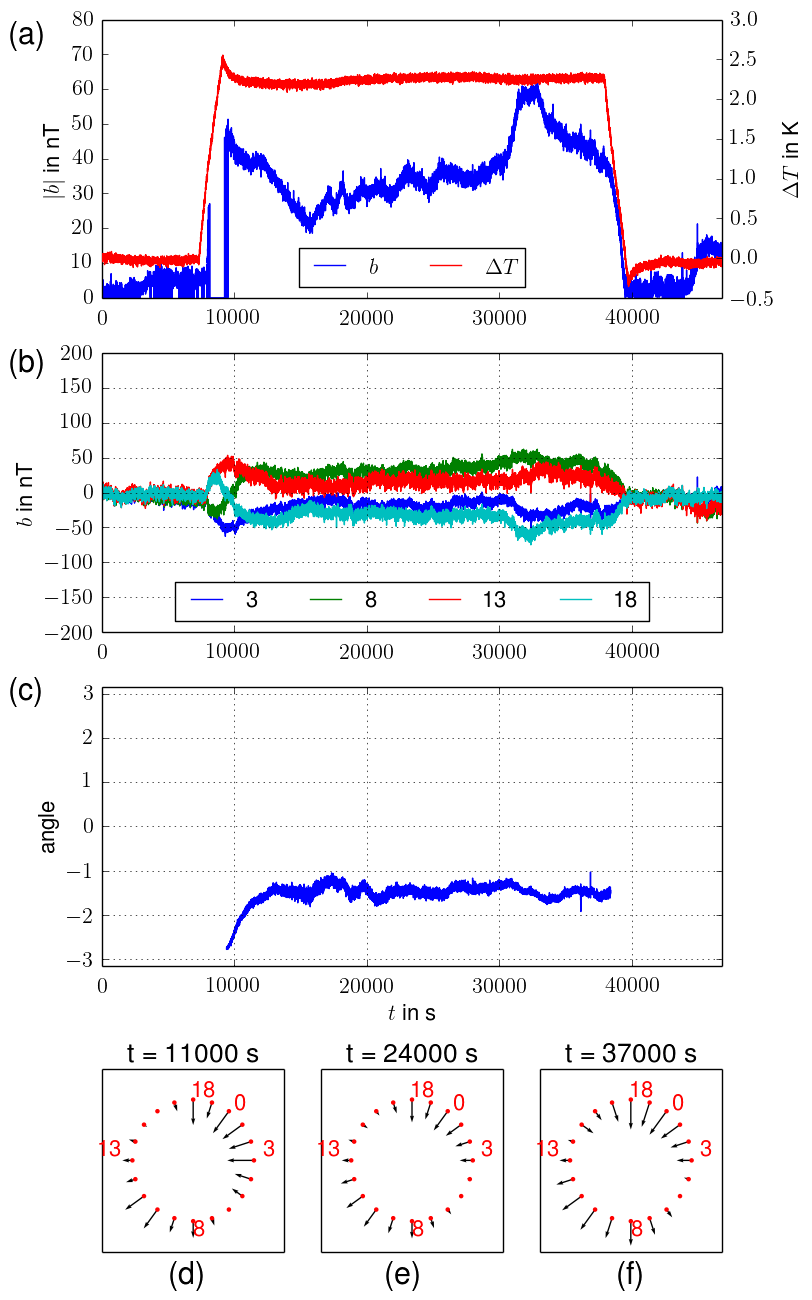
Figure 3: Measurements for $\Delta T=2.2$ K. (a) Temperature difference and amplitude $|b(t)|$ of the sine fit to the 20 measured magnetic fields. (b) Signals of sensors 3,8,13,18 which are separated by 90^∘. (c) Inferred angle $\phi_{0}(t)$. (d,e,f) All 20 magnetic signals as measured at three different snapshots.

For this comparably low temperature difference, we obtain relatively smooth data which indicate a fairly stable LSC that is basically pinned at a certain angle, around which it performs weak oscillations. Such a pinning of the LSC at some particular angle had also been observed by Cioni et al. [6] who had attributed it to weak inhomogeneities of the experimental set-up (in particular, the heating system).

The impression of a ”quiet” LSC is also supported by Fig. 4 which shows the histograms of the amplitude $|b(t)|$ of the 20 measured magnetic fields (a), and the histogram of the angle $\phi_{0}(t)$ (b).

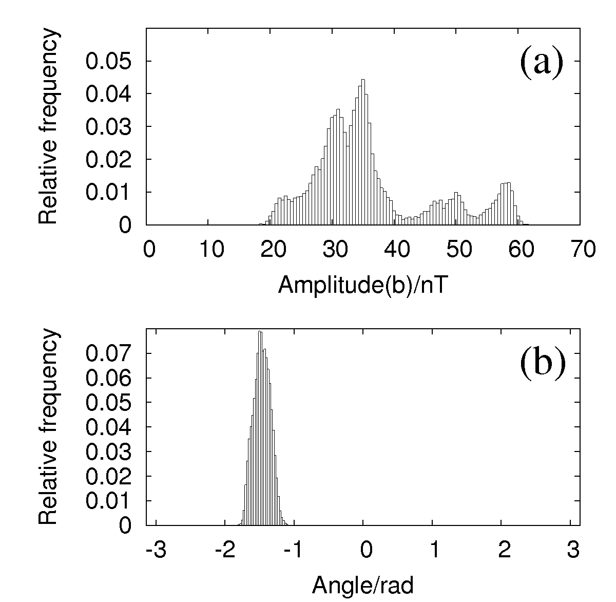
Figure 4: Histogram of the amplitude of the sine fit to the 20 measured magnetic fields (a), and of the angle $\phi_{0}$ of the LSC (b), for $\Delta T=2.2$ K.

Fig. 5 is an enlarged section of Fig. 3 for the time-interval $30000...30500$ s. Sensors 8 and 13, in particular, show a regular oscillation, whose sharp frequency $f=0.0185$ Hz can be identified in the Fourier transform of the time series (see Fig. 18 further below). This frequency, which lays in the typical range of the turn-over frequency $f_{turnover}\approx v_{LSC}/(4H)$ of the LSC, very likely corresponds to either a torsional or a sloshing mode [13]. Given the restriction of our sensor data to only one height, we refrain here from trying to distinguish between the two modes, and leave that for future work.

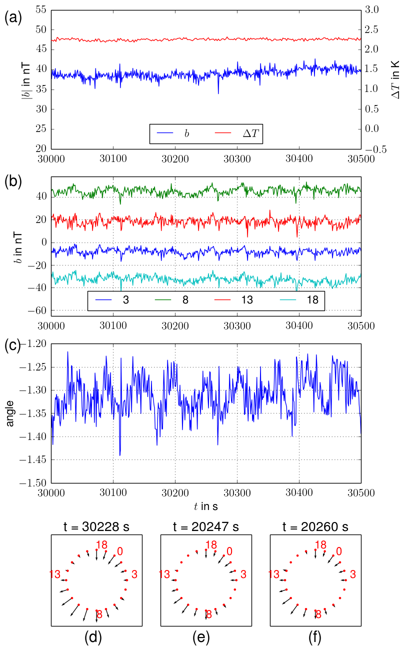
Figure 5: As in Fig. 3, but restricted to the period $30000...30500$ s. A dominant oscillation with a frequency of 0.0185 Hz is clearly visible in the sensor and angle data.

4.2 Experiments at $\Delta T=5.3$ K

New effects come into play when increasing the temperature difference to $\Delta T=5.3$ K. Fig. 6 shows again the complete time-line of the experiment, which reveals significantly stronger variations of the LSC. This is also visible in the histograms (Fig. 7), in particular in the broader distribution of the amplitude.

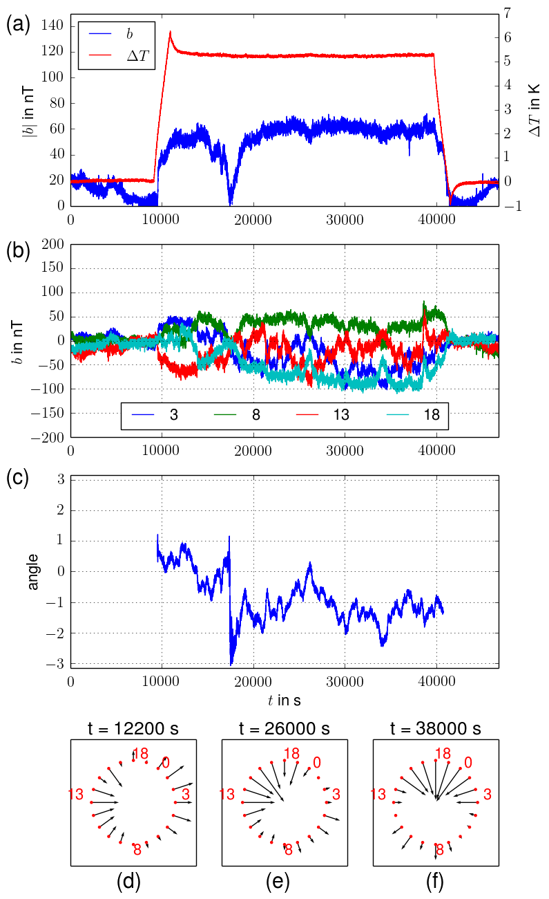
Figure 6: As in Fig. 3, but for $\Delta T=5.3$ K.

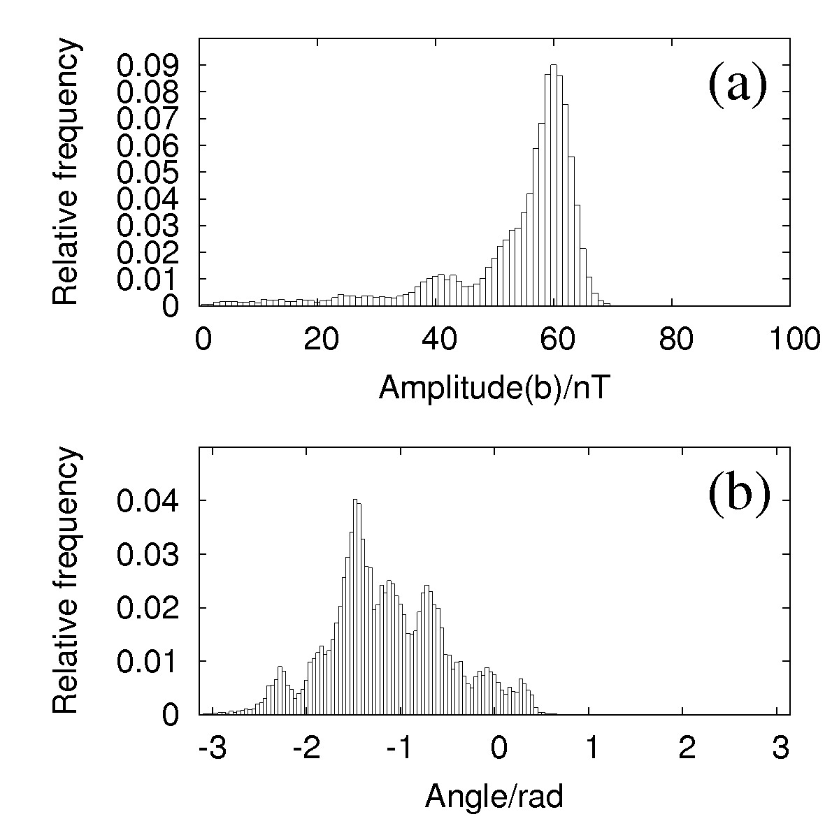
Figure 7: As in Fig. 4, but for $\Delta T=5.3$ K.

An interesting detail of this experiment is exhibited in Fig. 8 which covers the time interval $14000...19600$ s. Around $t=17500$s we observe a vanishing of the amplitude of the magnetic fields, which clearly indicates a ”cessation” of the LSC as it had been described previously by various authors [8, 10]. After this cessation, the LSC starts again at another angle (Fig. 8c).

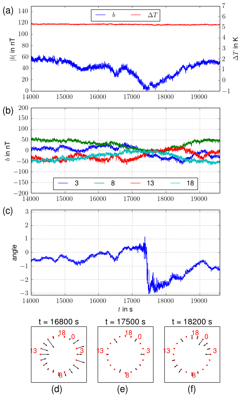
Figure 8: As in Fig. 6, but restricted to the period $14000...19600$ s. The flow ceases at around $t=17500$ s.

4.3 Experiments at $\Delta T=12.5$ K

A somewhat different behavior is observed at $\Delta T=12.5$ K. Fig. 9a indicates a rather constant amplitude of the fields (and hence of the intensity of the LSC), with just a moderate reduction close to the end of the experiment. However, the individual sensor signals (Fig. 9b) point to strong fluctuations of the angle of the LSC, which is quantified in Fig 9c and illustrated in the three snapshots of Figs. 9d,e.

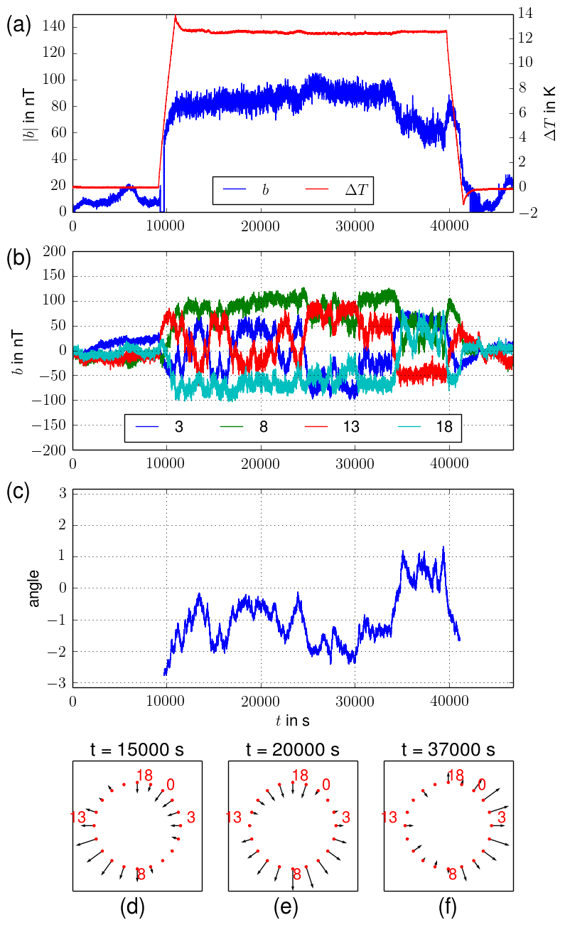
Figure 9: As in Fig. 3, but for $\Delta T=12.5$ K.

The corresponding histograms show indeed a remarkable constant amplitude (Fig. 10a) and a kind of tri-modal distribution of the angle (Fig. 10b).

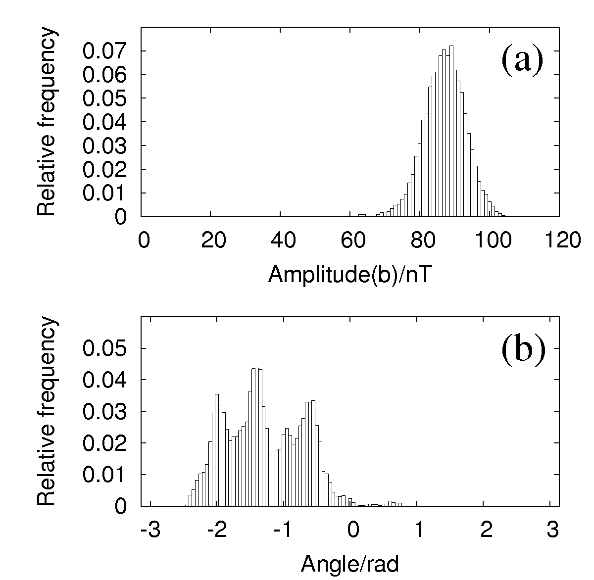
Figure 10: As in Fig. 4, but for $\Delta T=12.5$ K.

A rather slow rotation of the angle by around 180^∘ can be identified in the details for the time-interval $32000...36000$ s, see Fig. 11.

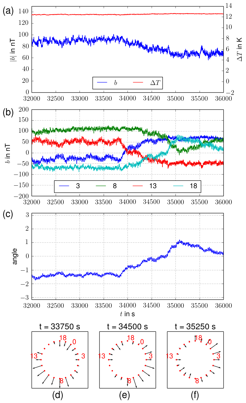
Figure 11: As in Fig. 9, but restricted to the period $32000...36000$ s. Note the rotation of the angle at around $t=34500$ s.

4.4 Experiments at $\Delta T=31.6$ K

Yet another feature appears at $\Delta T=31.6$ K (Fig. 12). Again, the amplitude of the field remains rather constant, while the individual fields and the angle undergo sudden jumps and reversals. The histogram (Fig. 13b) shows now a sort of bi-modal behavior of the angle with two dominant angles which are opposite to each other.

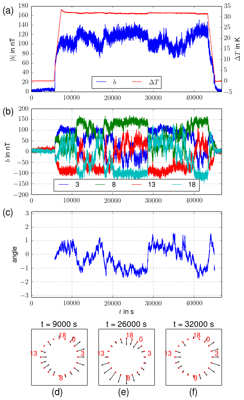
Figure 12: As in Fig. 3, but for $\Delta T=31.6$ K.

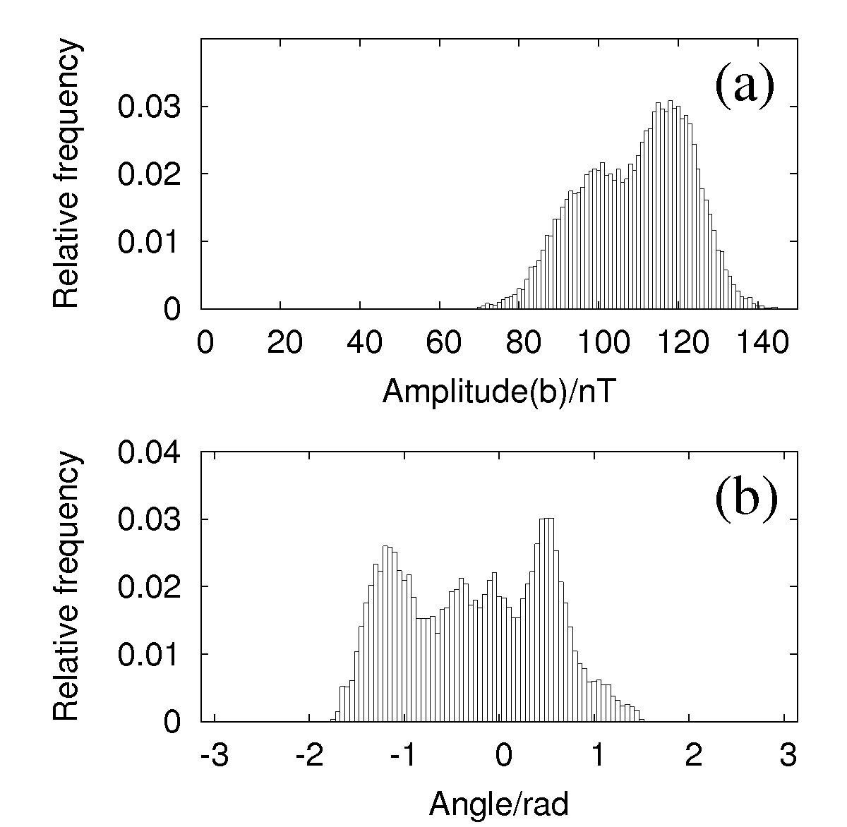
Figure 13: As in Fig. 4, but for $\Delta T=31.6$ K.

A typical reversal between the two angles, which relies on a fast rotation instead of a cessation, is illustrated in detail in Fig. 14.

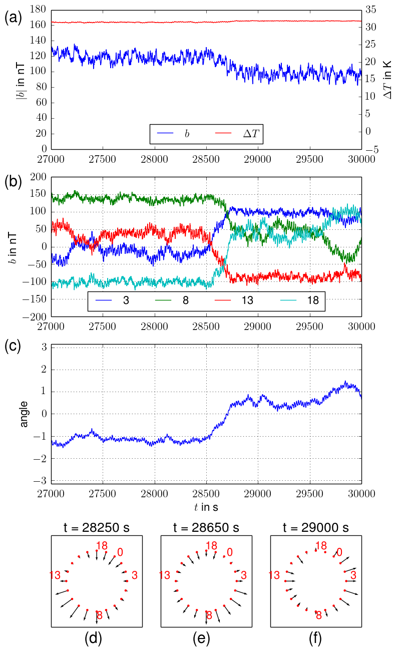
Figure 14: As in Fig. 12, but restricted to the period $27000...30000$ s. Note the fast rotation of the angle starting at $t=28500$ s.

4.5 Experiments at $\Delta T=80.8$ K

In contrast to the shorter experiments discussed above, the run at $\Delta T=80.8$ K has been carried out over a time interval as long as $50$ h. Over this period, the amplitude of the fields does not change very much, while the individual fields and the angle of the LSC undergo again strong variations (Fig. 15). The histogram (Fig. 16) shows now a sort of bi-modal behavior of both the amplitude and the angle, which on closer inspection even seem to be correlated.

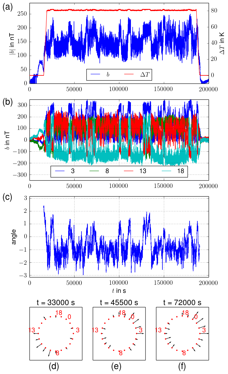
Figure 15: As in Fig. 3, but for $\Delta T=80.8$ K.

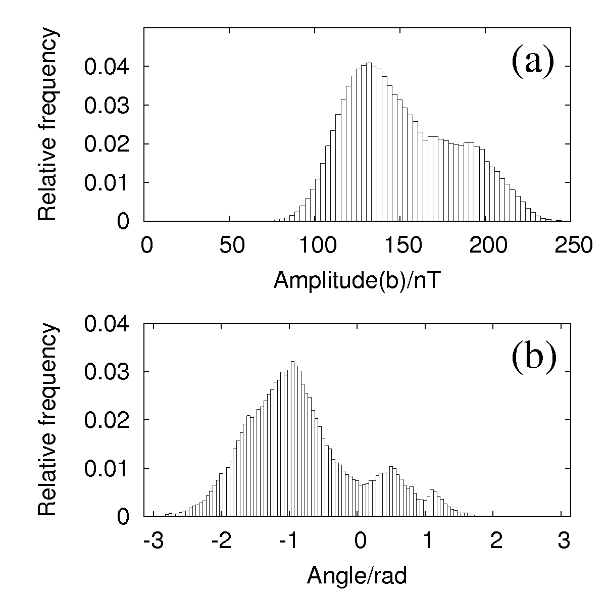
Figure 16: As in Fig. 4, but for $\Delta T=80.8$ K.

Fig. 17 shows the details of an ”excursion” of the angle of the LSC.

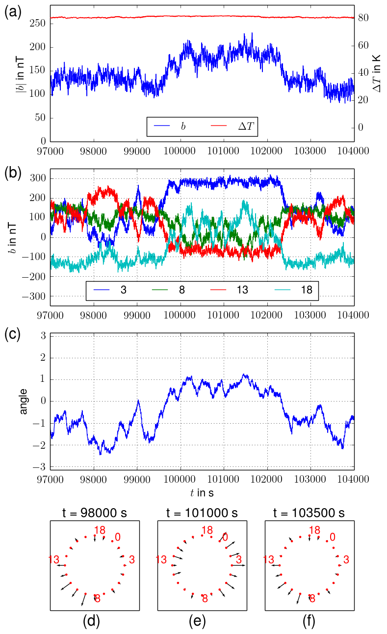
Figure 17: As in Fig. 15, but restricted to the period $97000...10400$ s. Note the ”excursion” of the angle during this period.

4.5.1 Summary of experiments

For five different values of $\Delta T$ (and, therefore, of $Ra$) the measured magnetic field perturbations have unveiled a variety of flow phenomena. These include a LSC that is pinned at some angle from were it undergoes slight oscillations which, very likely, correspond to torsional and/or sloshing modes. In all experiments the frequencies of these modes turned out to be quite sharp. This is illustrated in Fig. 18 which shows the spectra for the signal of sensor 8 (a), for the amplitude of all 20 sensor data (b), and for the angle $\phi_{0}$ of the LSC (c). Whereas the main peaks of the torsional/sloshing mode are clearly visible in all three features, some interesting distinctions can be made. For example, the peak of the amplitude for $\Delta T=12.5$ K is rather weak, while the corresponding peak of the angle is both strong and sharp. This is in agreement with the histograms in Fig. 10. Somewhat opposite to this is the behavior at $\Delta T=5.3$ K, which shows a weaker oscillation of the angle, but a more pronounced fluctuation of the amplitude (see also Fig. 7).

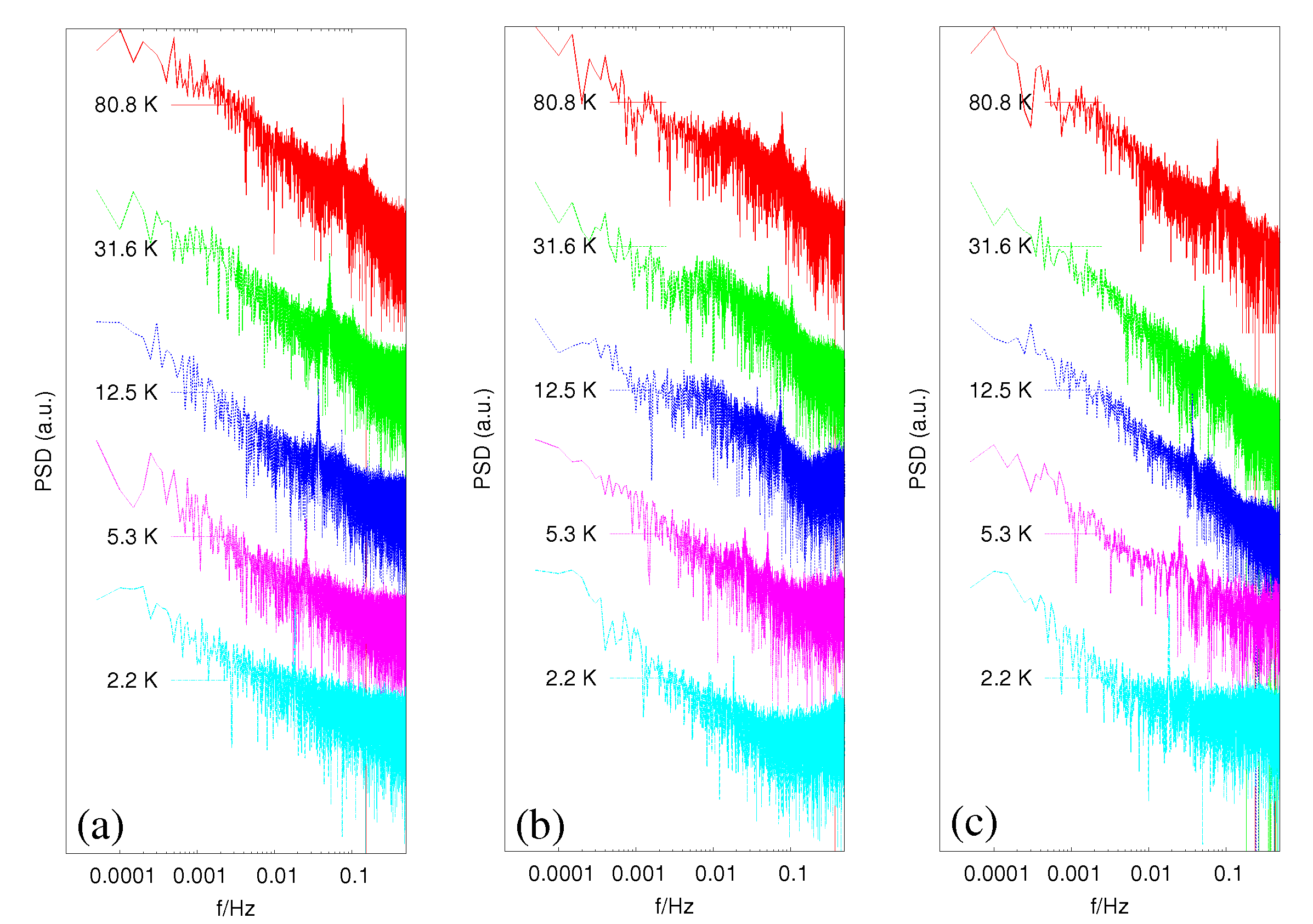
Figure 18: Spectra for the five runs with different temperature differences. (a) Spectra of the signal of sensor 8. (b) Spectra of the amplitude of the sine fit to the 20 measured signals. (c) Spectra of the angle of the LSC as determined from the 20 sensors. Note that the signals underlying all spectra were equally restricted to the interval $t=15000...35000$ s (even if the long measurements at $\Delta T=80.8$ K would have allowed for a much longer interval). The PSD is given logarithmically in arbitrary units, and the individual curves have been shifted appropriately for the sake of better visibility.

Based on a total of 14 experiments (from which we have discussed only five in detail), the dependence of the dominant frequency on $\Delta T$ is summarized in Fig. 19. The fit curve of these values is $f=0.013\Delta T^{0.401}$ which turns out to be in reasonable agreement with a corresponding result of Cioni et al. [6] who had derived a relation $2\pi f=0.47\kappa Ra^{0.424}$. The remaining difference of the exponent might be due to the partial cooling of the top, and/or to the temperature dependence of various material parameters which modifies, in particular for higher $\Delta T$, the simplified linear relation between $\Delta T$ and $Ra$.

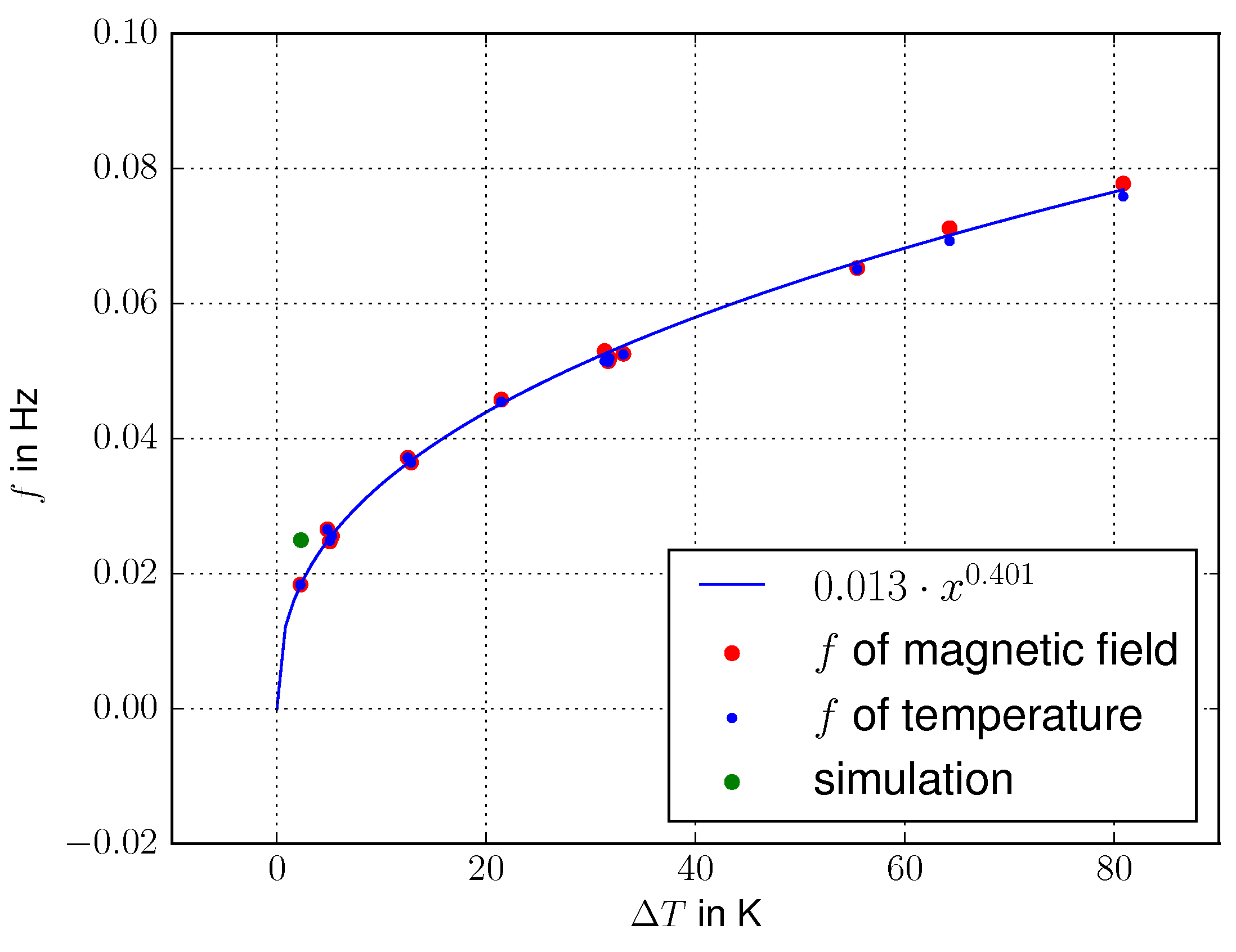
Figure 19: Dependence of measured frequencies on $\Delta T$, and the corresponding fit curve $f=0.013\Delta T^{0.401}$. The measurements were done simultaneously with the CIFT system (red) and with temperature sensors (blue). One single simulated frequency (green) fits well into the overall picture.

Apart from this general dominance of the high frequency modes, the experiments at larger $\Delta T$ show further effects, such as one (single !) cessation as observed for $\Delta T=5.3$ K, and the more frequent reversals at even higher $\Delta T$. The additional ”bulge” of the amplitude spectrum around $f\sim 0.01$ Hz, which becomes visible for $\Delta T=31.6$ K and $\Delta T=80.8$ K (Fig. 18b), indicates the appearance of low-frequency fluctuations of the LSC intensity, perhaps even a bi-modal behavior as also suggested in Fig. 16a.

4.6 Flow reconstructions

The presented measurements show that, despite of their weakness, the flow induced magnetic fields can be safely measured, and that the time-dependence of the LSC can be reliably determined. While a full three-dimensional reconstruction of the flow would require a second primary field to be applied in horizontal direction, and also more sensors to be distributed at different heights, we can still try to reconstruct the flow from just the 20 measurements at hand.

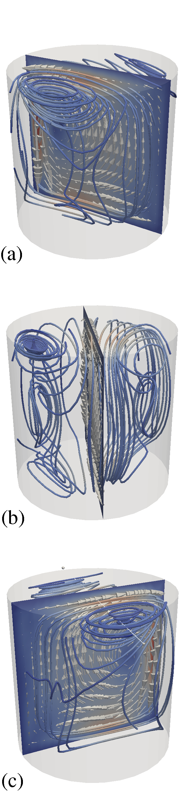
Figure 20: CIFT-reconstructed velocity for $\Delta T=31.6$ K, at the instants $t=28250$ s (a), $t=28650$ s (b), and $t=29000$ s (b), corresponding to the three measurements shown in Figs. 14d,e,f, respectively.

As an example we use here the three data snapshots from Figs. 14d,e,f, whose CIFT-reconstructions are shown now in Figs. 20a,b,c, respectively. Apart from some unrealistic eddy structures at the top (which are likely artifacts due to the missing magnetic field information at that height as seen in Figs. 2g,f), the global rotation of the LSC becomes clearly visible.

5 Conclusions

In this paper, we have demonstrated the viability of CIFT for measuring the LSC in liquid metal convection without any contact with the melt and without disturbing the homogeneous thermal boundary conditions at top and bottom. Even by only measuring the flow induced magnetic fields for one single (vertical) applied magnetic, it was possible to identify the direction and the dynamics of the LSC.

If a second magnetic field were applied to the convecting liquid, the full three-dimensional, time-dependent flow in the cylinder could be reconstructed with even better quality, although perhaps not with the very high empirical correlation coefficient as obtained, in the numerical part of this paper, for the time-averaged velocity. For this enhanced measurement configuration, we still have to find an optimum number and spatial distribution of sensors. One of the purposes of such an enhancement would also be to distinguish between torsional and sloshing modes of the LSC. The application of low-frequency AC fields, and the use of (gradiometric) pick-up coils, could further improve the robustness and technical applicability of the method.

6 References

References

- [1] L.P. Kadanoff, Turbulent heat flow: structure and scaling, Phys. Today 54 (2001) 34-39.
- [2] G. Ahlers, S. Grossmann, D. Lohse, Heat transfer and large scale dynamics in turbulent Rayleigh-Bénard convection, Rev. Mod. Phys. 81 (2009) 503-537.
- [3] R. Krishnamurti, L.N. Howard, Large-scale flow generation in turbulent convection, Proc. Natl. Acad. Sci. 78 (1981) 1991-1985.
- [4] M. Sano, X.-Z. Wu, A. Libchaber, Turbulence in helium-gas free convection, Phys. Rev. A 40 (1989) 6421-6430.
- [5] T. Takeshita, T. Segawa, J.A. Glazier, M. Sano, Thermal turbulence in mercury, Phys. Rev. Lett. 76 (1996) 1465-1468.
- [6] S. Cioni, S. Ciliberto, J. Sommeria, Strongly turbulent Rayleigh-Bénard convection in mercury: comparison with results at moderate Prandtl number, J. Fluid Mech. 335 (1997) 111-140.
- [7] H.-D. Xi, S. Lam., K.-Q. Xia, From laminar plumes to organized flows: the onset of large-scale circulation in turbulent thermal convection, J. Fluid Mech. 503 (2004) 47-56.
- [8] E. Brown, G. Ahlers, Rotations and cessations of the large-scale circulation in turbulent Rayleigh-Bénard convection, J. Fluid Mech. 568 (2006) 351-386.
- [9] C. Resagk, R. du Puits, A. Thess, F.V. Dolzhansky, S. Grossman, F.F. Araujo, D. Lohse, Oscillations of the large scale wind in turbulent thermal convection, Phys. Fluids 18 (2006) 095105.
- [10] H.-D. Xi, K.-Q. Xia, Cessations and reversals of the large-scale circulation in turbulent thermal convection, Phys. Rev. E 75 (2008) 066307.
- [11] D. F nfschilling, G. Ahlers, Plume motion and large scale circulation in a cylindrical Rayleigh-Bénard cell, Phys. Rev. Lett. 92 (2004) 194502.
- [12] H.-D. Xi, S.-Q. Zhou, T.-S. Chan, K.-Q. Xia, Origin of temperature oscillation in turbulent thermal convection, Phys. Rev. Lett. 102 (2009) 044503.
- [13] E. Brown, G. Ahlers, The origin of oscillations of the large-scale circulation of turbulent Rayleigh-Bénard convection, J. Fluid Mech. 638 (2009) 383-400.
- [14] A. Muiznieks, A. Krause, B. Nacke, Convective phenomena in large melts including magnetic fields, J. Cryst. Growth 303 (2007) 211-220.
- [15] A. Cramer, M. Röder, J. Pal, G. Gerbeth, A physical model for electromagnetic control of local temperature gradients in a Czochralski system, Magnetohydrodynamics 46 (2010) 353-361.
- [16] Y. Tasaka, K. Igaki, T. Yanagisawa, T. Vogt. T. Zürner, S. Eckert, Regular flow reversals in Rayleigh-Bénard convection in a horizontal magnetic field, Phys. Rev. E 93 (2016) 043109.
- [17] F. Stefani, G. Gerbeth, A contactless method for velocity reconstruction in electrically conducting fluid, Meas. Sci. Techn. 11 (2000) 758-765.
- [18] F. Stefani, T. Gundrum, G. Gerbeth, Contactless inductive flow tomography, Phys. Rev. E 70 (2004) 056306
- [19] M. Ratajczak, T. Gundrum, F. Stefani, T. Wondrak, Contactless inductive flow tomography: brief history and recent developments in its application to continuous casting, J. Sensors 2014 (2014) 739161.
- [20] P. C. Hansen, Analysis of discrete ill-posed problems by means of the L-curve, SIAM Rev. 34 (1992) 561-580.
- [21] T. Wondrak, V. Galindo, G. Gerbeth, Th. Gundrum, F. Stefani, K. Timmel, Contactless inductive flow tomography for a model of continuous steel casting, Meas. Sci. Technol. 21 (2010) 045402.
- [22] T. Wondrak, S. Eckert, G. Gerbeth, K. Klotsche, F. Stefani, K. Timmel, A. Peyton, N. Terzija, W. Yin, Combined electromagnetic tomography for determining two-phase flow characteristics in the submerged entry nozzle and in the mould of a continuous-casting model, Metal. Mater. Trans. B 42 (2011) 1201-1210.
- [23] T. Wondrak, S. Eckert, V. Galindo, G. Gerbeth, F. Stefani, K. Timmel, A.J. Peyton, W. Yin, S. Riaz, Liquid metal experiments with swirling flow submerged entry nozzle, Ironmaking and Steelmaking 39 (2012) 1-9.
- [24] F. Stefani and G. Gerbeth, On the uniqueness of velocity reconstruction in conducting fluids from measurements of induced electromagnetic fields, Inverse Probl. 16 (2000) 1-9.
- [25] J. Baumgartl, A. Hubert, and G. Müller, The use of magnetohydrodynamic effects to investigate fluid flow in electrically conducting melts, Phys. Fluids A 5 (1993) 3280-3289.
- [26] D.V. Berkov and N.L. Gorn, Reconstruction of the velocity distribution in conducting melts from induced magnetic field measurements, Comp. Phys. Comm. 86 (1995) 255-263.
- [27] F. Stefani, G. Gerbeth, K.-H. Rädler, Steady dynamos in finite domains: an integral equation approach, Astron. Nachr. 321 (2000) 65-73.
- [28] M. Xu, F. Stefani, and G. Gerbeth, The integral equation method for a steady kinematic dynamo problem, J. Comp. Phys. 196 (2004) 102-125.
- [29] T. Wondrak, F. Stefani, T. Gundrum, G. Gerbeth, Some methodological improvements of the contactless inductive flow tomography, Int. J. Appl. Electromagn. Mech. 30 (2009) 225-264.
- [30] Y. Plevachuk, V. Sklyarchuk, N. Shevchenko, S. Eckert, Electrophysical and structure-sensitive properties of liquid Ga-In alloys, Int. J. Mater. Res. 106 (2015) 66-71.
- [31] M. Ratajczak, T. Wondrak, T. Zürner, F. Stefani, Enhancing robustness and applicability of contactless inductive flow tomography, 2015 IEEE Sensors (2015) 7370342.