Visualization and Analysis of Large-Scale, Tree-Based, Adaptive Mesh Refinement Simulations with Arbitrary Rectilinear Geometry

Abstract

We present here the first systematic treatment of the problems posed by the visualization and analysis of large-scale, parallel adaptive mesh refinement (AMR) simulations on an Eulerian grid.

When compared to those obtained by constructing an intermediate unstructured mesh with fully described connectivity, our primary results indicate a gain of at least 80% in terms of memory footprint, with a better rendering while retaining similar execution speed.

In this article, we describe the key concepts that allow us to obtain these results, together with the methodology that facilitates the design, implementation, and optimization of algorithms operating directly on such refined meshes. This native support for AMR meshes has been contributed to the open source Visualization Toolkit (VTK).

This work pertains to a broader long-term vision, with the dual goal to both improve interactivity when exploring such data sets in 2 and 3 dimensions, and optimize resource utilization.

1 Introduction

1.1 Preamble

Massive numerical simulations are nowadays routinely run on petascale supercomputers such as Tera100 and the pre-exascale Tera1000 tera:CEA . Among simulation codes, those using adaptive mesh refinement (AMR) are especially efficient at tracking fine details within very large domains of interest. AMR enables a trade-off between numerical accuracy, memory footprint, and computational cost, by allowing for mesh refinement (and coarsening) in sub-regions of the simulation. Recent large scale simulations have reached ten trillion cells on a regular Eulerian grid woodward:12 . This pioneering work, representative of what will be “everyday” tomorrow exascale computing, showed that it might however be either impossible to store due to a too large number of elements, or would be computationally too expensive to post-process.

Figure 1: Visualization of supersonic shockwave drag, simulated on a tree-based AMR mesh.

These difficulties can be alleviated by refining the original mesh only where needed, while retaining coarser elements wherever local feature scales permit. Of course, this approach is limited to those specific physical problems where the meaningful phenomena are spatially localized. This is the case, for example, in astrophysics ramses:02 , transient wave propagation lomov:05 , or shock wave computation bale:02 ; berger:11 , illustrated in Figure 1, all cases where some appropriate coarsening criterion can also be easily defined.

Since the first description of an AMR methodology with the Berger-Oliger berger:84 type, several implementations have been proposed and developed. It is beyond the scope of this article to provide an in-depth comparison of block structured (also known as patch-based) versus tree-based (also known as point-wise structured) AMR methodologies. Nonetheless, in order to fully understand the motivations and constraints of the work presented hereafter, one must be aware that the fundamental difference between the two approaches is, essentially, a trade-off between memory footprint, and complexity of processing algorithms. Specifically, ceteris paribus, a typical tree-based AMR grid will occupy much less memory estate than its block structured equivalent, at the cost of higher processing time as a result of more complicated algorithms. In fact, this dichotomy between methods arises from the more general opposition between implicit and explicit representations, with the ensuing consequences when storing, as opposed to processing, the resultant data objects. It is worth noticing here that the FLASH framework flash:00 offers both options, although this is actually done with two different underlying codes: Chombo (block structured) and Paramesh (tree-based).

Block structured AMR will not be discussed in the rest of this article; the interested reader can refer in particular to the Chombo pages for more details chombo:overview . Our interest instead focused on the analysis of data sets produced by tree-based AMR codes. Several codes pertain to this group, for instance starting with successive refinement in octants (therefore producing octrees) of an initial root cell as done in RAMSES ramses:02 , or using a uniform, structured grid of root cells as done in RAGE/SAGE gittings:08 or HERA jourdren:05 , the tree-based AMR hydrodynamics simulation code developed at CEA.

1.2 Scope

We begin, in §2, by providing the background and context for this work, analyzing the challenges posed to scientific visualization by tree-based AMR simulations. As a result, we propose our global vision for addressing these challenges in an exascale perspective. However, the scope of this article is limited to the foundational aspects of this vision, by means of laying out the necessary data structures as well as the methodology to optimally process these.

What the reader will get from reading §3 is a full understanding of our novel data structures, which we implemented in VTK avila:10 . Wherever necessary, based in particular on acquired experience with large-scale data sets, we mention changes to claims or hypotheses which we had made in earlier work carrard:imr21 .

We then study in §4 the method we designed to operate on these data objects, with a particular emphasis on execution speed, in order to maintain interactivity even with the largest data sets that can be stored on currently available hardware.

We illustrate this methodology in §4.7, with a case of particular interest, namely iso-contouring, which is arguably one of the most widely used visualization techniques. It is also the most complicated, amongst all algorithms we have devised and implemented so far for our tree-based data sets, due to the intrinsic complications that arise from the very topological nature of iso-manifolds.

In §5, we examine the validity of our claims relative to performance with a set of tests, that are representative of the scientific simulation data sets we wish to address.

Finally, we conclude this article by examining to what extent the work presented in these pages covers what we initially intended to do. We subsequently discuss how future work will be articulated with what has been achieved so far, in order to achieve our long-term vision.

2 Context

2.1 Problem Statement

In order to exploit the massive data sets produced by the various numerical simulation codes of CEA, our visualization team developed the Large Object Visualization Environment (Love) aguilera:07 ; love:12 , a dedicated parallel visualization tool. It based on VTK/ParaView, an open-source, C++ set of libraries an applications for scientific data visualization and analysis supporting many data types and featuring hundreds of algorithms, with thousands of users in the global scientific community.

One approach for the visualization and analysis of AMR data sets with VTK is to use its native unstructured grid data objects. One obvious advantage of this method is to make available the wealth of existing filters already available in VTK for such data sets (e.g., cutting, clipping, iso-contouring, etc.). However, the additional memory requirements that arise from converting a mostly implicit data object into a fully explicit one rapidly become prohibitive as the size of the grid grows. Furthermore, when the cells of an AMR mesh are directly used as unstructured element inputs (quadrilaterals or hexahedra) of an algorithm such as iso-contouring, topological irregularities resulting in strong visual artifacts such as gaps may appear. These are caused by the topology of AMR meshes, which have partly connected vertices (“T-junctions”) when they contain neighboring cells at different refinement levels. Linear interpolation, commonly used by visualization algorithms, produces discontinuities across T-junctions, ultimately resulting in incorrect visualizations.

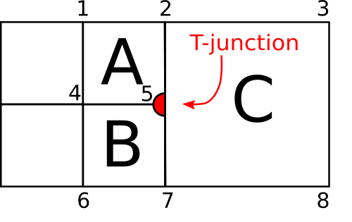
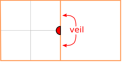
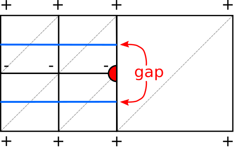
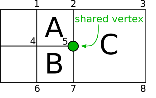
Figure 2: Top: AMR grid converted into: (left) a quadrangle mesh with a T-junction at point 5, which is shared by A and B but not by C, and (right) a generic unstructured mesh where vertex 5 is shared by pentagon C as well as quadrangles A and B. Middle: outside boundary (orange) computed over these 2 meshes; a topological artifact (veil) is caused by the T-junction (left), but not in the conforming, generic mesh (right). Bottom: linear iso-contour (blue) computed over theses 2 meshes, between vertex values above ($+$) or below ($-$) a given value; dashed gray lines represent possible triangulations used by the contouring algorithm.

The latter problem is further explicated in dimension 2 by Figure 2, where the top row represents an AMR grid with 5 cells. On the left, the cells are considered as the elements of an unstructured quadrilateral mesh: by construction, quadrangle C does not have any reference to vertex 5, creating a T-junction along edge 2–7. On the right, the cells are now viewed as arbitrary polygons, with pentagon C sharing vertex 5 with quadrilaterals A and B, hence eliminating the T-junction. Attempting to extract the outside boundary of the quadrilateral mesh results in a topological artifact, called a veil, whereas the outside boundary is correctly extracted on the polygonal mesh. Similarly, the effect of linear iso-contouring on both constructions, when cell values are above or below a given iso-value are shown in the bottom row. The T-junction on the left causes a gap in the iso-contour, because the algorithm cannot detect a contour intercept along edge 2–7 of cell C. Meanwhile, the same contouring algorithm is able correctly process the generic cells, and produces a correct iso-contour without false gaps.

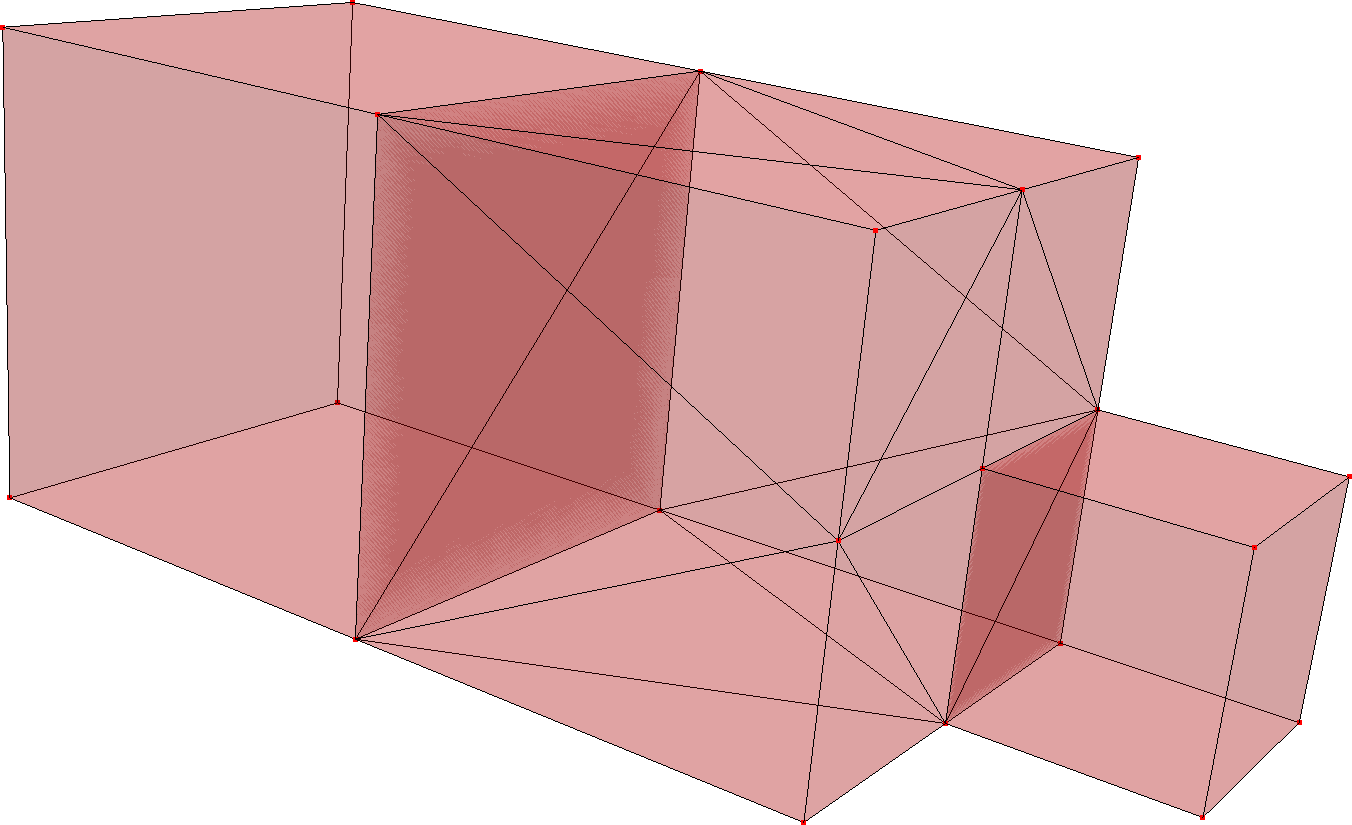
Figure 3: Top row, left: one generic cell located between 2 hexahedra, resulting in the appearance of extraneous veils being generated by the VTK geometry filter; right: all cells are generic and the boundary is correctly extracted by the filter. Bottom row: outside boundary of a bi-material 3D AMR simulation; left: extraneous veils appear when the filter is applied to a mixed-cell conforming unstructured mesh; right, the boundary is correctly extracted with all generic cells.

The Hercule I/O library developed at CEA hercule:12 supports such conversion from AMR grids into unstructured, conforming meshes. Prior to 2012, this was the only option available to visualize the tree-based AMR data sets produced at CEA. In addition to the already discussed performance limitations, using this approach also comes at the price of reduced interactivity because of I/O latency.

Furthermore, VTK does not support well the mixing of hexhaedral elements with generic cells as illustrated in Figure 3, left. Specifically, when attempting to extract the outside surface of the unstructured mesh with mixed cells, the subdivision of the generic cells by VTK results in incompatible tessellations across neighboring element faces. Although it is possible to resolve this problem by using only generic cells, as shown in Figure 3, right, but the computational and memory costs quickly become prohibitive for realistically-sized meshes.

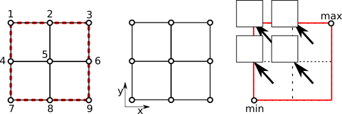
Figure 4: Two different representations of the same mesh: explicit unstructured representation (left), versus AMR description (right). The red color coding indicates the root cell, which is stored in the AMR representation, but not in the unstructured mesh.

It is easy to illustrate, for instance with the simple example depicted in Figure 4, the dramatic inefficiency of using explicit unstructured meshes to represent AMR grids. Considering a quadrilateral in dimension 2, decomposed into 4 sub-elements, it is straightforward to devise a corresponding tree-based AMR representation using $4$ floats for the extremal coordinates of the grid and $1$ Boolean value to indicate that the quadrangle is subdivided. Meanwhile, an explicit unstructured representation of the same requires $9\times 2=18$ floats for the vertex coordinates, as well as $4\times 4=16$ integers to describe the connectivity of the $4$ cells. Therefore, the AMR description reduces the memory footprint of almost a full order of magnitude for this simple case alone.

VTK has long provided some support for block-structured AMR data sets. Prior to 2012, it also offered very limited support for a particular case of tree-based AMR with a single-root octree object yau:83 .

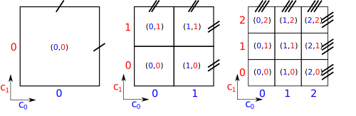
Figure 5: The 3 allowed AMR subdivision patterns in dimension $2$: without refinement ($f=1$, left), binary subdivision ($f=2$, center), and ternary subdivision ($f=3$, right), with respective numbers of children equal to $1$, $4$, and $9$. In dimension 3 these translate respectively into $1$, $8$, and $27$ children.

Furthermore, simulation codes such as HERA use either binary or ternary subdivision schemes when refining meshes, i.e., with branching factor $f\in\{2;3\}$ along each dimension of the grid. This is illustrated by Figure 5 in dimension $2$. In general, in dimension $d$, refining a cell results in obtaining $f^{d}$ subchildren (sub-cells). Any post-processing methodology designed to handle the results of such simulations must therefore be able to accommodate, not only the usual binary trees, quadtrees and octrees, but also more exotic ternary trees. Finally, another constraint to be taken account is the fact that AMR simulation codes used at CEA are run in parallel, with the corresponding data sets being distributed over many thousands of compute nodes. These codes balance computational sub-domains by allocating the root cells in the grid of trees, resulting in individual AMR trees that are never shared between different compute nodes. Traversal objects for such grids of trees must therefore be carefully designed in order to a priori allow for extremely unbalanced trees structures between various areas of the overall domain.

2.2 Vision

Our global, long-term vision for tree-based AMR visualization and analysis can be articulated as follows:

1. Propose a novel VTK data object to support all requested tree-based features, that is both memory-efficient and able to convert such objects into conforming meshes. This is to allow for the direct utilization of the wealth of existing unstructured mesh algorithms when explicitly requested.

2. Design and implement visualization and analysis algorithms that are specific to the primary tree structure, as needed by actual users, with a strong emphasis on performance. In our vision, this optimization of execution speed is best achieved by using specialized constructs called cursors and supercursors.

3. Optimize rendering speed, in order be able to maintain interactivity when visualizing the largest possible tree grids that can be contained in memory. A possible approach could be to take advantage of the tree structure of the grids, to allow for level-of-detail culling relative to the size of the rendering window, screen resolution, view and camera position, etc.

4. Qualitatively improve the final rendering with, e.g., mapping, texture splatting or ray tracing techniques specifically tailored for the tree-based AMR objects.

5. Design and implement a way to pass object information, so a reader specific to tree-based AMR grids be able to limit actual reading and storing of those parts of the entire grid that are explicitly needed by filters and rendering (such as maximum depth of refinement and bounding box).

6. Define a serialization specification for these structures, and develop I/O classes implementing it. Such a serialization protocol will also improve current parallel load balancing schemes by allowing for communication of large sub-grids in small messages.

7. Expand the range of supported tree-based AMR data sets; envisioned objects include grids that have many root cells but a small number of refinement levels or, conversely, that only have a very small number of root cells with many refinement levels. Such extensions would have to be achieved while maintaining the same goal of memory footprint minimization and execution speed maximization.

8. Expand the current post-processing paradigm to include concurrent approaches based on in situ and in transit processing. Such a data-centric approach would allow for increased spatial and temporal resolutions for post-processing purposes, reduced I/O costs, and significant decrease of time from data to insight. This would therefore alleviate increasing difficulties encountered by AMR simulation analysts caused by the current need to save a sufficient amount of raw solution data to persistent storage.

We acknowledge that some of these items are mutually independent, and thus do not have to be executed in the order of the list. However, [a] and [b] constitute the necessary foundation of the whole; this article is therefore focused on these two first steps.

3 Foundations

Neither of the features for tree-based AMR grids, necessary per the requirements detailed in §2, were supported by VTK prior to 2012. We therefore decided to design, and implement, what was then the first of its kind support for such data sets. This preliminary work was released as a set of new classes in VTK; we also briefly described its governing principles in carrard:imr21 . However, we never provided a comprehensive description of the corresponding data objects, and how they relate to the class of AMR meshes of interest in our applications. In addition, several years have passed since this first approach to the problem, and our ideas and implementations have matured and solidified. We therefore think that the time has come to provide an in-depth exposition of the foundations necessary to achieve our vision outlined above.

3.1 Vertices, Graphs, and Trees

It is beyond the scope of this article to provide an extensive picture of graph nomenclature and classification; the interested reader can refer, e.g., to bondy:11 for a systematic treatment of the theory of graphs. The fundamental building blocks of our trees are vertices, which can also be implemented as data objects containing various quantities of interest, such as simulation data, and mesh topology or geometry attributes. Given a set of vertices $V$, we then define an undirected edge as a pair set of vertices, with the following requirements for the set of all undirected edges:

1. be connected, i.e., any two vertices are connected by a path of adjacent edges, and

2. not contain any cycle, i.e., a set of edges forming a closed polygon.

In addition, one (and only one) vertex is chosen in $V$ to be the root. In this setting, the directed edges are immediately deduced from the undirected ones with the implicit ordering based on distance from the root, in the sense of number of edges needed to transitively connect to it. Note that this is implicit ordering is indeed unambiguous: on one hand, thanks to the connectivity axiom (i), any vertex in ${V}$ can always be connected to the root with a finite subset of undirected edges, called a path. Furthermore, this path is unique: otherwise, a plurality of such paths would contradict the acylicity axiom (ii); one can then define a unique depth as being the number of edges in this path. Finally, at least one vertex does not have any directed edge leaving it, and any vertex that has this property is called a leaf; all non-leaf vertices are called strict nodes.

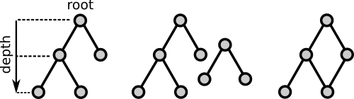
Figure 6: Three different types of graphs: tree (left); not connected graph (center), not a tree but nonetheless a forest; and a graph containing a cycle (right), therefore not a tree. We decide to always show the root at the top.

What matters most for a correct understanding of this article, is to pay attention to the fact that typical usage of the term tree in Computer Science refers to a directed, rooted, acyclical graph, whereas in Mathematics it is more broadly understood as an undirected, transitive, acyclical graph. The double $(V,E)$, where $E$ is the set of all directed edges, is the definition of a tree to be used thereafter. A handful of examples and counter-examples are provided in Figure 6; note that, for concision, we never represent the directionality of the edges, for it is implicit as we use the convention to always represent a tree with its root at the top. We also decide to always horizontally align vertices that have the same depth.

3.2 The Hyper Tree Object

We now introduce the concepts specific to our work, and in particular the following, for which there are different definitions in the literature:

Definition 1

A hyper tree object (shorthand hypertree) in dimension $d\in\mathbb{N}^{*}$ with branching factor $f\in\mathbb{N}^{*}$, is a type of data set that can be represented as a tree, and where each strict node has exactly $f^{d}$ children. In addition, primary attributes of this data set are attached to the vertices of the tree.

Remark 1

The range of AMR grids we want to support for our applications is limited to the possible combinations of $d\in\{1;2;3\}$ and $f\in\{2;3\}$. The corresponding objects are called, in dimension $1$, bintrees ($f=2$) and tritrees ($f=3$), in dimension $2$, quadtrees ($f=2$) and $9$-trees ($f=3$), and in dimension $3$, octrees ($f=2$) and $27$-trees ($f=3$).

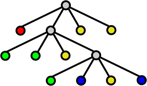
Figure 7: Left: a $2$-dimensional AMR mesh obtained with 3 levels of successive binary refinements of a quadrilateral; right: the corresponding hypertree representation. Colors are used to represent the attribute values attached to mesh cells.

There is a trivial bijection between hypertree objects and tree-based AMR meshes descending from a unique root cell: for instance, each leaf of a hypertree object $\mathcal{H}$ represents exactly one mesh cell that is not refined, whereas strict nodes in $\mathcal{H}$ are bijectively associated with all coarse cells (i.e., cells in the mesh that are subdivided). This bijective construction is illustrated with the case of a quadtree in Figure 7. Note that this AMR mesh does not have attribute values attached to coarse cells, whence the gray color in the corresponding strict tree nodes. However, it is possible to assign attribute values to strict nodes, and in fact some CEA simulations codes compute attribute values at coarse cells. Furthermore, coarse cell attributes can be computed during post-processing, e.g. for level-of-detail (LOD) purposes. Last, as will be seen later in this article, we exploit this capability to store attribute values at strict nodes in the aim of optimizing tree traversals for some classes of filters.

Regarding the geometry of a hypertree object, this work addresses the case of AMR meshes embedded in the $3$-dimensional Euclidean space $\mathbb{R}^{3}$, irrespective of their actual dimensionality. We thus do not provide support for higher dimension meshes, which are not needed by current AMR simulation codes. Another consequence is that we do not handle planar nor linear AMR grids natively; rather, they are always viewed as a 3D object with one or two fixed coordinates. This might appear as a sub-optimal setting, which it is in some very limited respect because, as we will see, coordinates do not have to be stored for all cells. But, on the other hand, VTK is optimized for dimension 3, and its rendering system does not provide a good way to co-mingle objects of different dimensionalities in a generic fashion. Furthermore, some of the visualization filters considered, and in some cases developed, produce AMR outputs that have lower dimensionality than the AMR inputs. Therefore, this trade-off appears to be the best one under the current circumstances: choice of the visualization library as well as range of potential data sets.

Because the considered AMR meshes are always rectilinear, the geometry of a hypertree object is implicitly but nonetheless unambiguously specified, given:

1. the origin $\overrightarrow{x}=(x_{0};x_{1};x_{2})\in\mathbb{R}^{3}$ of the root node;

2. the size $\overrightarrow{s}=(s_{0};s_{1};s_{2})\in\mathbb{R}^{3}$ of the root node; and

3. the direction (resp. normal, first axis) vector $\overrightarrow{v}\in\mathbb{R}^{3}$ of the root node in dimension $1$ (resp. $2$, $3$).

We made the additional design choice to natively support only axis-aligned tree-based AMR meshes, because VTK has a generic approach to supporting geometric transformations such has translations, rotations, and homothecies. This allows us to use an orientation value $o\in\mathbb{N}$ only, in order to specify the direction of the axis along which a 1-dimensional AMR mesh is aligned, or the normal to the plane inside which a 2-dimension mesh is contained, in order to specify the embedding into $\mathbb{R}^{3}$. If $d=3$, the convention is that $o=0$ as this value is not used anyway. Last, thanks to the size vector $\overrightarrow{s}$, supported AMR geometries are therefore not limited to unit segments, squares and cubes, but also include arbitrary segment lengths and rectangular shapes. Using these notations, the triple $(\overrightarrow{x};\overrightarrow{s};o)\in(\mathbb{R}^{3})^{2}\times\mathbb{N}$ is called the $3$-dimensional embedding of the considered hyper tree.

3.3 Mapping and Indexing

No particular indexing is assumed in tree structures in general, for it depends on the particular traversal scheme utilized to visit tree vertices and index them accordingly. However, we need to have a consistent mapping scheme, in order to unambiguously map AMR meshes in the class we want to address, into hypertree objects. In Figure 7 for instance, implicit orderings of mesh cells and of tree vertices were used, in order to map one into the other. It is natural, following the flow in which mesh refinement is performed, to convention that mesh cells as well as tree vertices are ordered by depth, root first, which is another way of saying that both mesh and tree are traversed by breadth-first search (BFS) bondy:11 traversal.

Meanwhile, because there is no unique order over $\llbracket 0;f\llbracket^{d}$, as soon as $d>1$, it is easy to convince oneself that choosing a particular BFS scheme amounts to determining a unique way to locally index the sub-cells obtained by refining a coarse cell $C$, called children cells of $C$. By definition, there are always $f^{d}$ such children cells to any coarse cells, which can each be uniquely identified in terms of the number of refinements at which they begin along each axis. The corresponding indices in $\llbracket 0;f\llbracket^{d}$, shown in Figure 5 in the case where $d=f=2$, are called the child coordinates. In order to generalize the construction illustrated in this example, to map an arbitrary AMR mesh into a hypertree, in an unambiguous manner, one needs to define a particular bijection from the $d$-dimensional Cartesian product $\llbracket 0;f\llbracket^{d}$ into the ordered set $\llbracket 0;f^{d}\llbracket$. For all our work, we decide to use the following convention:

Definition 2

The hypertree child index map $\Upphi_{d,f}$, with $(d,f)\in{\mathbb{N}^{*}}^{2}$ is the lexicographic order over $\llbracket 0;f\llbracket^{d}$.

It is beyond the scope of this article to discuss the lexicographic order over Cartesian products in a detailed way; suffices to know that it is the analog to the lexicographic order over finite words in a finite alphabet (the dictionary order) and that it indeed provides a total order. In addition, one has the following property, whose proof is left to the interested reader as an exercise (by recurrence over $d$):

Proposition 1

Given child coordinates $(c_{0},\dots,c_{d-1})$ in dimension $d$:

$$\Upphi_{d,f}(c_{0},\dots,c_{d-1})=\sum_{k=0}^{d-1}c_{k}f^{k}.$$

$$\begin{array}[]{@{}r|cc@{}}1&6&7\\ 0&4&5\\ \hline\cr c_{2}=1&0&1\end{array}$$

$$\begin{array}[]{@{}r|cc@{}}1&2&3\\ 0&0&1\\ \hline\cr c_{2}=0&0&1\end{array}$$

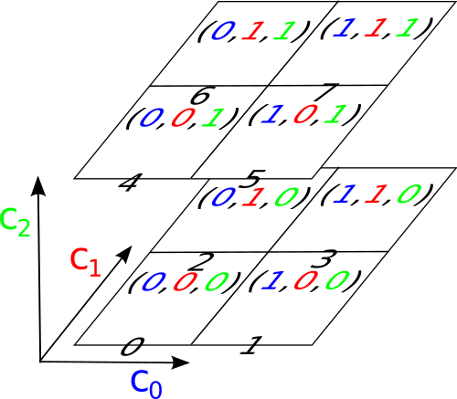
Figure 8: The hypertree child index map in the $3$-dimensional binary case ($d=3$, $f=2$).

The index maps for $d=1$ are simply the identities over $\llbracket 0;f\llbracket$. For the values of $d$ and $f$ that are of practical interest to us, the $(c_{0},c_{1},c_{2})$ tables are given in Figure 8 for $f=2$, and by the following tables for $f=3$:

$$\begin{array}[]{@{}r|ccc@{}}2&6&7&8\\ 1&3&4&5\\ 0&0&1&2\\ \hline\cr c_{2}=0&0&1&2\end{array}\quad\begin{array}[]{@{}r|ccc@{}}2&15&16&17\\ 1&12&13&14\\ 0&9&10&11\\ \hline\cr c_{2}=1&0&1&2\end{array}\quad\begin{array}[]{@{}r|ccc@{}}2&24&25&26\\ 1&21&22&23\\ 0&18&19&20\\ \hline\cr c_{2}=2&0&1&2\end{array}$$

When considering only the 2 tables with $c_{2}=0$ amongst the above, one obtains the corresponding maps for $d=2$.

3.4 The Hyper Tree Grid Object

In order to account for a broad category of tree-based AMR grids, including those that do not have uniform geometry along each axis, or whose initial refinement pattern is not that of hypertree, we introduced a broader-scoped object in 2012, which have since deeply modified and are discussing fully now.

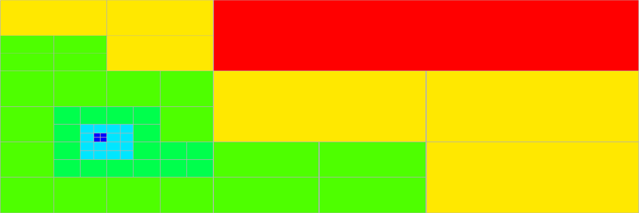
Figure 9: A $2$-dimensional AMR mesh obtained with 4 levels of successive binary refinements of $3\times 2$ rectilinearly aligned hypertree objects with different sizes along each axis.

Definition 3

Let $\mathcal{H}$ and $\mathcal{H}^{\prime}$ be two hypertree objects, with same dimension $d\in\{1;2;3\}$ and branching factor $f\in\mathbb{N}^{*}$, with respective $3$-dimensional embeddings $(\overrightarrow{x};\overrightarrow{s};o)$ and $(\overrightarrow{x}^{\prime};\overrightarrow{s}^{\prime};o^{\prime})$. If

$$\exists k\in\{0;1;2\}\quad\left\{\begin{array}[]{l}x_{k}^{\prime}=x_{k}+s_{k}\\ \forall l\in\{0;1;2\}\setminus{\{k\}}\;(x_{l}^{\prime},s_{l}^{\prime})=(x_{l},s_{l})\end{array}\right.$$

and, when $d\neq 3$, $o^{\prime}=o$, we say that $\mathcal{H}^{\prime}$ is rectilinearly consecutive to $\mathcal{H}$ for component $k$, denoted $\mathcal{H}\underset{k}{\prec}\mathcal{H}^{\prime}$.

Intuitively, what this means is that the outside boundary of $\mathcal{H}\cup\mathcal{H}^{\prime}$ is a line segment in dimension $1$, a rectangle in dimension $2$, and a rectangular prism in dimension $3$, with origin and orientation equal to those of $\mathcal{H}$, and size vector as well, except for its $k$ component which is equal to $\overrightarrow{s_{k}}+\overrightarrow{s_{k}}^{\prime}$. For example, Figure 9, are shown $6$ binary hypertree objects in dimension $2$, arranged in to have rectilinear consecutiveness for components $0$ and $1$.

Given any triple $t\in\mathbb{N}^{3}$, we denote $\Uppi{t}$ the product of its components, and $\llbracket{t}\llbracket$ the set of triples $t^{\prime}\in\mathbb{N}^{3}$ such that $t^{\prime}<t$ in the lexicographic sense. For example,

$$\llbracket{(3;2;2)}\llbracket=\big{\{}\{0;0;0\};\{0;0;1\};\{0;1;0\};\dots;\{2;1;1\}\big{\}}.$$

We now introduce our main object:

Definition 4

A hyper tree grid object (shorthand hypertree grid) in dimension $d\in\{1;2;3\}$ with branching factor $f\in\mathbb{N}^{*}$ and extent $E\in{\mathbb{N}^{*}}^{d}\times\{1\}^{3-d}$, denoted $\mathcal{G}_{E}^{d,f}$, is a type of data set comprising $\Uppi{E}$ hyper tree objects in dimension $d$ and with branching factor $f$, denoted $\mathcal{H}_{i,j,k}$ where $(i;j;k)\in\llbracket{E}\llbracket$, such that

$$\forall(i;j;k)\in\llbracket{E}\llbracket\;\left\{\begin{array}[]{lcl}i+1<E_{0}&\Rightarrow&\mathcal{H}_{i,j,k}\underset{0}{\prec}\mathcal{H}_{i+1,j,k}\\ j+1<E_{1}&\Rightarrow&\mathcal{H}_{i,j,k}\underset{1}{\prec}\mathcal{H}_{i,j+1,k}\\ k+1<E_{2}&\Rightarrow&\mathcal{H}_{i,j,k}\underset{2}{\prec}\mathcal{H}_{i,j,k+1}\end{array}\right.$$

In addition, primary attributes of this data set are attached to the individual hypertrees.

Given an arbitrary hyper tree grid object $\mathcal{G}_{E}^{d,f}$, we denote $\mathcal{H}_{i,j,k}^{d,f}$ the hyper tree object with discrete coordinates $(i;j;k)\in\llbracket{E}\llbracket$ and call it the constituting hypertree of $\mathcal{H}_{E}^{d,f}$ at position $(i;j;k)$. Under the assumptions of Definition 4 regarding $d$, $f$, and $E$, we have:

Proposition 2

The outside boundary of a hyper tree grid object $\mathcal{G}_{E}^{d,f}$ is a $d$-dimensional rectangular prism, uniquely determined by the $3$-dimensional embeddings of its constituting hypertree objects.

Proof

Without loss of generality, it is sufficient to prove this assertion in dimension $3$: the result in dimension $2$ (resp. $1$) ensues by setting $E_{2}=1$ (resp. $E_{1}=E_{2}=1$). By definition, given any 2 integers $a$ and $b$ such that $(1,a,b)\in\llbracket{E}\llbracket$, $\mathcal{H}_{0,a,b}^{d,f}\underset{0}{\prec}\mathcal{H}_{1,a,b}^{d,f}$ and, for all $i\in\llbracket 0;E_{0}-1\llbracket$, $\mathcal{H}_{i,a,b}^{d,f}\underset{0}{\prec}\mathcal{H}_{i+1,a,b}^{d,f}$. Therefore, by recurrence, the outside boundary $R_{a,b}$ of $\cup_{i<E_{0}}\mathcal{H}_{i,a,b}$ is a rectangular prism with origin and size equal to those of $\mathcal{H}_{0,a,b}$, with the exception of the first component of its size vector, that is equal to the sum of the first components of the size vectors along the first axis.

Applying the same argument to such stacks, with the form $\cup_{i<E_{0}}\mathcal{H}_{i,a,b}$, that are consecutive along the second axis, one obtains that the outside boundary $R_{b}=\cup_{a}R_{a,b}$ of $\cup_{i<E_{0},j<E_{1}}\mathcal{H}_{i,j,b}$ is also a rectangular prism, with origin and size equal to those of $\mathcal{H}_{0,0,b}$, with the exception of the first and second components of its size vector, that are equal to the sums of the first and second components of the size vectors along the first and second axes, respectively.

Finally, stacking consecutive blocks $\cup_{i<E_{0},j<E_{1}}\mathcal{H}_{i,j,b}$ that are consecutive along the third axis, one finally obtains the outside boundary $R=\cup_{b}R_{b}$ of $\mathcal{G}_{E}^{d,f}$, a rectangular prism, with origin equal to that of $\mathcal{H}_{0,0,0}$, and with size vector whose components are the sums of the corresponding components of the size vectors along the 3 axes, respectively. ∎

Remark 2

Applying the same argument to the origin vectors of the constituting hypertrees shows that these are exactly the vertex coordinates of a rectilinear grid, whose elements are exactly the bounding boxes of said hypertrees. It is therefore not necessary to explicitly store the $\Uppi{E}$ geometric embedding triples (i.e., $2d\Uppi{E}$ floats and $\Uppi{E}$ integers) to describe the geometry of the hypertree grid. Rather, it is sufficient to describe it implicitly by storing one coordinate array per dimension and a single orientation for the entire grid, at a much smaller total cost between $d(\sqrt[d]{\Uppi{E}}+1)$ (best case: $\mathcal{G}_{(a,a,a)}^{3,f}$) and $\Uppi{E}+5$ (worst case: $\mathcal{G}_{(a,1,1)}^{d,f}$) all hypertrees consecutive along a single direction) floats, plus a single integer.

Finally, a map providing a direct look-up from the local index $n_{\mathrm{l}}$ of a vertex inside the constituting hypertree $(i;j;k)\in\mathbb{N}^{3}$, into the global index $n_{\mathrm{g}}$ of this vertex relative to $\mathcal{G}_{E}^{d,f}$ as a whole, is needed in order to retrieve attribute values at any given vertex. Such a map thus must take the following form:

Definition 5

The global index map $\Upgamma_{d,f,E}$ of a hypertree grid $\mathcal{G}_{E}^{d,f}$ is an injective map:

$$\begin{array}[]{rccl}\Upgamma_{d,f,E}:&\mathbb{N}^{4}&\longrightarrow&\mathbb{N}\\ &(n_{\mathrm{l}};i;j;k)&\longmapsto&n_{\mathrm{g}}.\end{array}$$

We hereafter freely identify any rectilinear, tree-based AMR meshes with its corresponding hypertree grid object, referring to this process as that of identification, so that it not be confused with that of duality which we are now going to discuss.

3.5 The Dual Mesh

In order to resolve the difficulties posed by AMR T-junctions, two different approaches are possible: one is to implement new processing algorithms specialized towards tree-based AMR grids, the other consists of transforming the AMR input into a conforming unstructured grid, allowing for reuse of existing algorithms. In earlier work carrard:imr21 (which, in our knowledge, is the only existing work in this field), we chose the latter approach, by the means of defining a dual grid construction, upon which all filters designed for vertex-centered attributes (i.e., iso-contouring) could natively operate when all variables are cell-centered. In this case, the visualization results are correct, provided the attributes correspond to variables values computed at cell centers – as opposed to averaged over the cell. That was a strong limitation of this approach, from its inception, as most cell-centered simulations use the latter rather than the former.

Nonetheless, this notion of duality remains a powerful conceptual tool when the considered visualization technique requires that the elements of a conforming mesh be generated, used, and disposed of, one at a time (as opposed to creating the entire mesh) In what follows, by mesh we refer to a polytopal cover of a finite, closed subset of an Euclidean space. The reader interested in an in-depth discussion of meshes, and how they relate to numerical simulations, can refer in particular to frey:08 .

Definition 6

Given $d\in\{1;2;3\}$ and a $d$-dimensional mesh $\mathcal{M}$, referred to as the primary mesh, we define its dual mesh $\mathcal{M}^{\ast}$ as follows:

1. to every $d$-dimensional cell $e\in\mathcal{M}$ is associated a dual vertex $e^{\ast}\in\mathcal{M}^{\ast}$, with coordinates those the isobarycenter of $e$;

2. to every vertex $v\in\mathcal{M}$ is associated a dual cell $v^{\ast}\in\mathcal{M}^{\ast}$, whose vertices are exactly the dual vertices $e_{i}^{\ast}\in\mathcal{M}^{\ast}$ such that $v$ is a vertex of $e_{i}$.

Depending on the value of $d$, dual edges and dual faces are defined as the $1$ and $2$ dimensional elements of the dual cells, respectively.

Remark 3

Note that this definition is not that of duality in the Delaunay-Voronoï sense delaunay:34 because, as a result of the finite extent of $\mathcal{M}$, there is no bijection between the vertices of $\mathcal{M}$ and the cells of $\mathcal{M}^{\ast}$ although, by construction, there is a bijection between the cells of $\mathcal{M}$ and the vertices of $\mathcal{M}^{\ast}$.

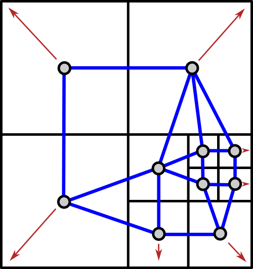
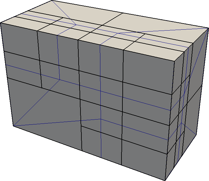
Figure 10: Left: a 2D ternary tree-based AMR mesh (in black), overlaid with its dual (in blue); arrows indicate how the dual vertices may be displaced to produce an adjusted dual. Right: a 3D binary tree-based AMR grid (in black) overlaid with its adjusted dual (in blue).

When applied to the case of AMR meshes, this definition must be understood in the sense that $\mathcal{M}$ only contains the non-refined cells (i.e. hypertree leaves), excluding all coarse cells (i.e. hypertree strict nodes). Furthermore, we often also use an adjusted dual $\varphi(\mathcal{M}^{\ast})$, where $\varphi$ is a geometric transformation that maps the vertices belonging to $\partial\mathcal{M}^{\ast}$, the boundary of $\mathcal{M}^{\ast}$, so that

$$\partial\varphi(\mathcal{M}^{\ast})=\partial\mathcal{M}.$$

Note that there is no unicity in the choice of $\varphi$; examples of this construction are provided, in dimension $2$ and  $3$, in Figure 10. Using the notion of conforming mesh in the sense of a polytopal covering where two $k$-dimensional items are either distinct or their intersection is exactly a shared $(k-1)$-dimensional item of the mesh, we have the following key result, whose proof is left to the reader as an exercise:

Proposition 3

If $\mathcal{M}$ is formed by the refined cells of a tree-based rectilinear AMR mesh, then $\mathcal{M}^{\ast}$ is a conforming mesh.

By definition, a T-junction is the topological configuration where two edges (i.e. $1$-dimensional mesh items) intersect at a vertex (i.e. a $0$-dimensional mesh item) which is not shared by both edges. Therefore, if a mesh has one T-junction, it is not conforming; by contraposition of Proposition 3, it follows that the problem of T-junctions as illustrated, e.g. in Figure 2, vanishes when replacing the primal AMR mesh with its dual or its adjusted dual (which does not modify the topology).

3.6 Cursors and Supercursors

We are now at a point where we can represent and store all tree-based, rectilinear AMR meshes we want to support. The question that immediately follows is that of operating on these, by means of appropriately designed hypertree grid filters. In order to do this, such filters must be endowed with an efficient way to both access and traverse hypertree grid objects. Because a hypertree grid $\mathcal{G}$ is inherently a list of hypertrees, it is only natural to iterate over these as a way to traverse $\mathcal{G}$ in its entirety. In general, depth-first search (DFS) traversal of trees is efficient, and is therefore our preferred modus operandi, whenever no other order of traversal is explicitly needed. Meanwhile, an algorithm that needs to iterate over all vertices of $\mathcal{G}$ will also typically need access to some of the information contained there, such as global indices allowing for attribute retrieval from data arrays. We thus introduce the following object:

Definition 7

A hypertree cursor is a structure pointing to a hypertree, that can both traverse it and access its vertex attributes.

A minimal hypertree cursor will therefore comprise a reference to the underlying hypertree, together with a stack-like data structure storing the path from the root to the current vertex, i.e. the vertex towards which the cursor is pointing. It will also be endowed with at least the two following operators:

ToParent():

move one vertex up in the tree, except if already at the root.

ToChild(i):

descend into the vertex with child index i (cf. Definition 2), relative to the vertex currently pointed at, except if already at a leaf.

Any actual implementation will also equip this structure with other operators such as data accessors, direct or indirect, to vertex attributes. Because the AMR meshes we want to address only have cell-wise attributes, the corresponding data arrays are all of equal length and allow for random access per cell index. In order to keep the hypertree cursor as lightweight as possible, we chose to provide only indirect access to attribute values, which can be achieved with a single instance variable storing vertex, and therefore mesh cell, indices into the corresponding data arrays. This turns into the requirement that attribute fields be all ordered in the same fashion, using the global indexing scheme (cf. Definition 5).

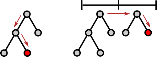
Figure 11: DFS traversal to the red-colored leaf, in a hypertree (left) and a hypertree grid (right).

However, because individual hypertrees are never used on their own but, rather, are always interlocked in a broader hypertree grid $\mathcal{G}$, the hypertree cursor is not sufficient to traverse $\mathcal{G}$. Rather, it must be enriched with additional topological information, allowing it to move from one tree root to the next, as if there were a meta-root vertex, from which all hypertree roots would descend. This means, in particular, that both ToParent() and ToChild() must be equipped with additional logic, in order to properly traverse across level $0$ cells. This is illustrated in Figure 11, showing the path taken by a hypertree cursor searching a vertex with a give attribute value, compared to that of a hypertree grid cursor doing the same inside a $2\times 1\times 1$ hypertree grid.

A hypertree cursor, extended to allow for traversal across a grid of hypertree objects, is naturally called a hypertree grid cursor.

Furthermore, many visualization filters require neighborhood information to perform their computations. For example, an outside boundary extraction filer, in dimension $3$, needs to know whether a given cell has neighbors across any of its faces, as a boundary face is generated if and only if it is not shared by two cells. In order to provide neighborhood information we devised and implemented the following compound structures:

Definition 8

A supercursor is a hypertree grid cursor keeping track of a neighborhood of cursors while traversing the hypertree grid.

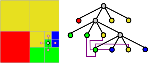
Figure 12: Left: $4$-neighborhood of a cell in a $3$-deep, $2$-dimensional binary AMR mesh; right: same neighborhood when mapped to the hypertree representation of the mesh.

For the sake of simplicity, let us consider the case of a hypertree grid containing a single hypertree. One such example is readily provided by the single-root AMR mesh of Figure 7, left. Let us then turn our attention to the single green cell that is to be found at the deepest refinement level: it has $4$ neighbor across its edges, marked by the cross-shaped structure in Figure 12, left. This same structure is then showed, to the right, after having been mapped onto the hypertree equivalent of the AMR mesh: the set of purple multi-lines connecting the green leaf at maximum depth to 4 other tree leaves is, effectively, the supercursor state when it points to the green leaf with depth 3. Implementing this supercursor thus entails providing the logic necessary to update these links, when moving vertically within a hypertree, as well as when moving horizontally from one hypertree root to a neighboring one in the Cartesian grid of roots.

Remark 4

It is important to note that a supercursor is not a hybrid DFS/BFS traversal structure: it can only retrieve information from the vertices to which it is linked, but it cannot directly traverse to them. The complexity and computational cost of a traversal object able to achieve that end would be prohibitive indeed.

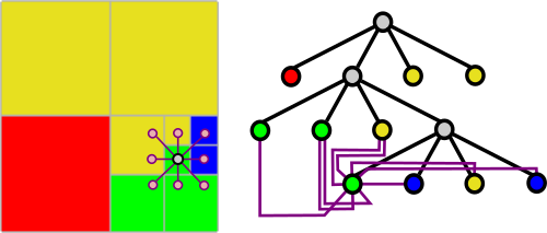
Figure 13: Left: $8$-neighborhood of a cell in a $3$-deep, $2$-dimensional binary AMR mesh; right: same neighborhood when mapped to the hypertree representation of the mesh.

Another complication arises from the fact that the notion of neighborhood itself is not invariant, but rather depends on the considered topology. In our case, choosing a topology amounts to defining a criterion to decide whether $2$ cells in an AMR mesh are connected. For instance, the already introduced hypertree and hypertree grid cursors are supercursors with respect to the discrete topology. In dimension $1$ (resp. $2$, $3$), another type of connectivity is called the $2$- (resp. $4$-, $6$-) connectivity, where two cells are connected if and only if their share a common vertex (resp., edge, face). This type of connectivity defines the corresponding $d$-dimensional Von Neumann neighborhood packard:85 .

Moreover, some algorithms need richer neighborhoods, expanding this criterion to include connectivity across mesh vertices for $d=2$, and also across mesh edges for $d=3$. For instance, in order to compute a dual cell associated with a given vertex $v$ of a primal cell $C$ in dimension $2$, it is necessary to iterate over all mesh cells that share $v$ with $C$, i.e., all those that are connected to $C$ either by an edge that contains $v$, or by $v$ alone. A Von Neumann neighborhood no longer suffices for this purposes. In dimension $3$, the problem is further compounded by the distinction between per-vertex, per-edge, and per-face connectivity. This defines the corresponding $d$-dimensional Moore neighborhood. Figure 13 illustrates the difference between these two neighborhood types in dimension $2$, with the Moore supercursor pointing to $3^{d}-1=8$ neighbors, of which only $2d=4$ belong to the Von Neumann neighborhood of Figure 12.

Note that, in dimension $1$, there is not distinction between von Neumann and Moore connectivities. Furthermore, in dimension $2$, these two are distinct but without any intermediate in the scale of connectivity pattern whereas, in dimension $3$ one could also consider 18-connectivity, i.e., where two mesh cells are connected if and only if they share a face or an edge (but a vertex only is not sufficient). However, we have not found so far any use case where this type of connectivity would be useful. Other types of neighborhoods could also be defined, e.g., with vicinity stencils spanning more that one cell on each side, as required by the considered algorithm.

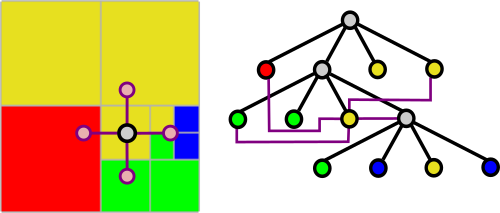
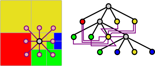
Figure 14: Von Neumann (top) and Moore (bottom) neighborhoods of a cell that has neighbors with greater depth, in a $3$-deep, $2$-dimensional binary AMR mesh.

However, the notion of vicinity of a cell is not always unambiguous. Specifically, given a cell $C$ at depth $\delta(C)$ in the mesh and one of its lower-dimensional entities $e$, define $\mathcal{N}(C,e)$ the set of all cells that are neighbors of $C$ across $e$ for the considered neighborhood type. When $\mathcal{N}(C,e)\neq\varnothing$, let $C^{\prime}\in\mathcal{N}(C,e)$ that has greatest depth in $\mathcal{N}(C,e)$. This cell $C^{\prime}$ is not necessarily unique, and only the following two cases thus may occur:

1. $\delta(C^{\prime})>\delta(C)$; in this case, $C^{\prime}$ is a smaller cell than $C$ and other cells with the same size may share entity $e$ with $C$ as well. The neighbor cell to $C$ is thus chosen to be the unique $C^{\prime\prime}$ in $\mathcal{N}(C,e)$ that has the same depth as $C$; this is illustrated in Figure 14.

2. $\delta(C^{\prime})\leq\delta(C)$; in this case, $C^{\prime}$ is a cell at least as large as $C$ and thus there can be no ambiguity for no other mesh cells may share $e$ with $C$ as well. In this case, and only in this case, $C^{\prime}$ is chosen to be the neighbor of $C$ in the supercursor.

Two important consequences result from the above: first, one same cell can appear more than once in the vicinity cursors; second, a neighbor of a leaf can be a coarse cell.

3.7 The Material Mask

Further complexity arises from the fact that AMR simulations results we wish to support can also distinguish between different materials participating in the simulation. We now focus on how we have enriched the hypertree grid object in order to both support this additional feature and at the same time take advantage of it even in the absence of a material specification to increase execution speed of some filters.

One first consideration is that the material properties are specified on a per-cell basis, for coarse as well as for refined cells. Furthermore, some simulations allow for the presence of two different materials in a same cell, hereby implying the existence of a material interface, which can be approximated using various techniques not discussed here. By design, a coarse cell in the AMR mesh exists if and only it has at least one leaf in its descent that contains the selected material. Although this can result in an incomplete AMR mesh, when compared to the whole computational domain, this trade-off is warranted by the fact that the analyst generally knows which materials are strictly necessary, and which ones can be ignored (e.g., vacuum, inert materials, etc.).

Our approach to handling the material, is to define an additional cell-wise attribute, call the material mask. In practice, this is a bit array, sized as the other attribute arrays of the considered hypertree grid, i.e., with a number of entries that are equal to the number of vertices (both strict nodes and leaves).

Our approach to processing hypertree grids with non-void material mask is to consider masked vertices, as well as all their descent, as being non-existent. As a result, a DFS traversal will stop its descent as soon as a masked tree vertex is encountered, irrespective of the fact that its parent cell is stricto sensu a strict node, hereby giving rise to a notion of lato sensu leaf: for all processing purposes, a strict vertex in the hypertree, whose children are all masked, is considered as a leaf node. Moreover, one masked tree vertex hides to processing algorithm the entirety of the sub-tree that descends from it. Nonetheless, the entirety of the hypertree grid remains represented.

This design constraint, arising from the very nature of the notion of material in an AMR mesh, must not only be accommodated, but can also be abused, by being used as a form of virtual decimation. This results in dramatically accelerating execution speed of hypertree grid filters, as they traverse an input mesh and obey some logic to decide whether an input cell with generate output items, or not. In other words, for the sake of performance, a material mask can be used to produce virtually decimated hypertree grids, at the expense of the additional memory required to store the hidden parts. In general, a material mask is an attribute with negligible relative memory footprint, for it only consumes one bit per tree vertex. However, the additional memory space required by the virtually decimated – but nonetheless truly represented – vertices might become prohibitive. An ideal use of this concept would therefore balance those two relative costs in an adaptive fashion and decide when actual decimation shall be executed.

4 Method

After having established the necessary foundations for our work, we now discuss the methodology that we used to turn this theoretical framework into an actual implementation. While §3 can be understood as a frame of reference that shall not evolve much in the future, the concrete methods discussed below are, by nature, subject to further improvements or revisions. In particular, the techniques which are discussed hereafter are already improvements upon earlier versions: we have completely revised our approach to utilizing the dual, as well as the design of supercursors, with respect to our our earlier presentation carrard:imr21 . We begin by describing our methodological choices for efficient representation and indexing of hypertrees and hypertree grids.

4.1 The Compact Representation

The ratio between the number of strict nodes to the total number of nodes remain within $[\tfrac{1}{1+f^{d}};\tfrac{1}{f^{d}}]$, an tends towards the upper bound of this interval as the number of nodes increases. It thus follows that the number of leaves dominates that of strict nodes. Which is why we sought to implicitly define the leaves, while explicitly storing in memory only the strict nodes. Such a compact representation still allows for traversal, at the cost of minimal additional processing when visiting the leaves due to their implicitness compensated by fewer cache missing.

In order to fully describe a hypertree, it is therefore sufficient that each strict node store one index to refer the first amongst its children, called the eldest child node. It is indeed sufficient to only store a reference to the eldest when all children of a given cell are created as once as a block of contiguous indices, at the end of the node array, instead of allocating memory for each child which might be non-leaf cell itself. Furthermore, the size of this block is constant and equal to $f^{d}$, by definition of a hypertree. In addition, because all of these children, child leaf or child strict node, have the same parent, it suffices that only the eldest child store its parent index. In fact, in order to retrieve the parent of any given node, only the extra step of finding the position of its eldest sibling is thus necessary.

Figure 15: Construction of a binary hypertree in dimension $1$: the order in which it is performed impacts the total memory footprint. At each step (#), the index in a square is that of the nodes being refined; indices underlined with a solid (resp. dashed) line represent allocated (resp. implicit) nodes.

Using short integers, of size 4 bytes (B), in order to store the parent index child, and denoting $m$ the number of its strict nodes, describing the topology of a hypertree thus costs at a minimum $4(m-1)$B for the parent indices of the eldest children and $4m$B for the indices of the eldest children themselves; this amounts to a total cost of $8m-4$ bytes if $m\in\mathbb{N}^{*}$. This theoretical minimum cost is rarely attained. The overall efficiency of this approach is very sensitive to the topological structure of the tree and the order in which it is traversed at construction time. This is illustrated in Figure 15: when the topological structure of the tree is created in DFS order, some unnecessary allocations (namely, for nodes 4 and 5) occur; in contrast, an optimal traversal only allocates space for strict tree nodes. This worst case occurs when the last refined cell is the one which is also the last entry during the penultimate refinement stage, the cost for parent indices can be as high as $4(m-1)(1+f^{d})$B.

One thus obtains the following bounds for the memory cost $C(m)$, expressed in bytes:

$$4(2m-1)B\leq C(m)\leq 4\left[1+(m-1)(1+f^{d})B\right].$$

Note that the lower bound indicated above is a theoretical memory footprint, with an ideal topology where all children of a strict node have the same type (either all strict nodes, or all leaves) and ideal implementation (the traversal strategy refines last all strict nodes than only have leaf children). Unfortunately, there is not a way to devise a traversal strategy that is optimal for all possible topological structure of trees.

When $n$ hypertrees are embedded inside a $d$-dimensional hypertree grid, $m\gg{n}$, this minimum cost becomes $4(2m-n)$B and is reached when at most one common depth level is partially refined across all hypertrees. The maximum cost occurs in both cases when only one hypertree is refined, and with the worst possible traversal; in this case, the cost is $4\left[n+(m-1)(1+f^{d})\right]$B for $m\in\mathbb{N}^{*}$. On the other hand, the memory footprint relative to the description of the spatial grid, using double precision floats for the coordinates, is least equal to $8\left(3+d\sqrt[d]{n}\right)B$ for a square or cubic grid, and at most $8(d+n+2)$B for a linear grid.

All lower bounds theoretical mentioned above are indeed very difficult to attain. But the lower bound defined for a topology is attain with the ideal implementation that it is therefore the responsibility of the developer to make this trade-off, depending on whether additional CPU processing is acceptable to achieve a better memory footprint, with potentially enormous gains. For instance, in the binary $3$-dimensional case, the memory gain factor between this AMR description and its explicit, unstructured all-hexahedral equivalent can range from $18$ to more than $80$.

4.2 The Global Index Map

A natural choice to build a concrete $\Upgamma_{d,f,E}$ is to combine a $0$-level indexing of the constituting hypertree roots with the child index maps in each of these hypertrees. For instance, the $0$-level indexing can be the lexicographic order in §3.3, applied to $\llbracket{E}\llbracket$. One can then set

$$\Upgamma_{d,f,E}(n_{\mathrm{l}};i;j;k)=n_{\mathrm{l}}+S_{i,j,k}$$

where $S_{i,j,k}$ is the global index start of the hypertree object at position ${i,j,k}$ in the Cartesian grid of hypertree objects. By construction, the restriction of $\Upgamma_{d,f,E}$ to any particular hypertree, being piece-wise affine with unit slope, is strictly increasing over $\mathbb{N}$ and therefore injective. Therefore, if the $S_{i,j,k}$ are chosen so that there be no overlap across the image spaces of these per-hypertree restrictions, then $\Upgamma_{d,f,E}$ as a whole is injective and thus satisfies the specification of Definition 5.

In this setting, the global index start of each constituting hypertree only needs to be stored as an integer offset, at the minimal additional cost of $8$B per hypertree. In practice, this can be achieved by constructing the hypertree grid one hypertree object at a time, and incrementing the global index start when moving to the next hypertree with the number of vertices in the last constructed hypertree.

It is important to note, however, that this method to build the global index map by means of assigning a global index start per constituting hypertree is in no way mandatory. Rather, our implementation provides the ability to specify an arbitrary version of $\Upgamma_{d,f,E}$; it is the responsibility of the developer to ensure that this map comply with the requirements of Definition 5. In addition, such an explicit definition increases the total memory footprint by the cost of representing as many integers as there are vertices in the hypertree grid.

4.3 The Virtual Dual

In order to support the widest variety of visualization algorithms, our first version of the hypertree grid object was implemented with a primal/dual API, because while some visualization filters work best processing dual grid cells, others can operate directly upon the primal cells. This double API thus provided visualization filters with the alternative to traverse hypertree grids through either primal or dual cells.

A first limitation of this design is its complexity, as two different outside-facing data structures must be maintained and kept consistent. In addition, dual grids have inherently a more complex topology than their corresponding primal tree grids. For instance, dual grids of $3$-dimensional tree-based AMR meshes contain pyramids and wedges, in addition to hexahedral cells. Moreover, the memory footprint of the dual has proven to become untenable when attempting to process realistically sized cases, for the dual must be represented explicitly (in the sense of fully described, unstructured grid), canceling all the benefits of tree-based storage.

Figure 16: Left: a $2$-dimensional tree-based AMR mesh $\mathcal{M}$ (gray), overlaid with $\mathcal{M}^{\ast}$ (blue), showing dual cell ownership by primal vertices with orange arrows; right: cursor indices in a $2$-dimensional Moore supercursor, used as tie-breakers for dual cell ownership amongst the deepest primal cells.

Algorithm 1 $\mathtt{IsOwner}(s,i)$

1:  $\delta\leftarrow\mathtt{GetDepth}(s)$

2:  $\omega\leftarrow\tfrac{3^{d}-1}{2}$

3:  for all $j\in\mathcal{\llbracket}{2^{d}}\llbracket$ do

4:     $k\leftarrow\mathtt{CornerNeighborCursorsTable}[d][i][j]$

5:     $c\leftarrow\mathtt{GetNeighbor}(s,k)$

6:     if $\mathtt{Masked}(c)\lor\neg\mathtt{IsLeaf}(c)\lor(k>\omega\land\mathtt{GetLevel}(c)=\delta)$ then

7:        return  $\mathtt{False}$

8:     end if

9:  end for

10:  return  $\mathtt{True}$

In order to avoid cell replication in the dual grid, our method assigns ownership of dual vertices to a single leaf, amongst the $2^{d}$ that potentially touch a primal vertex in dimension $d$: specifically, ownership of the dual cell is assigned to the deepest of these leaves, breaking ties in favor of the one that has the greatest cursor index relative to the others. Specifically, the function that determines ownership of the dual cell at any corner $i\in\llbracket{2^{d}}\llbracket$ of an arbitrary leaf cell, at which a Moore supercursor $s$ is centered, is explicated in Algorithm 1 and illustrated in Figure 16, left. The $3$-dimensional integer array called $\mathtt{CornerNeighborsCursorTable}$ is a table that provides, given a $d$-dimension Moore supercursor and a corner index, the indices of the cursors that surround said corner. that surround centered at a cell is a corner-to-leaf traversal table to retrieve the $2^{d}$ indices of all the cell cleaves touching a given corner of a given cell. For example in dimension $2$, as illustrated in Figure 16, right,

$$\mathtt{CornerNeighborCursorsTable}[2][0] =\{0;1;3;4\}$$

$$\mathtt{CornerNeighborCursorsTable}[2][1] =\{1;2;4;5\}$$

$$\mathtt{CornerNeighborCursorsTable}[2][2] =\{3;4;6;7\}$$

$$\mathtt{CornerNeighborCursorsTable}[2][3] =\{4;5;7;8\}.$$

Although this method keeps the additional memory footprint at the strict minimum, by avoiding dual cell duplication, it is not sufficient to prevent memory overruns even with relatively modestly-sized AMR meshes as a result of the unstructured nature of the dual mesh. As a result, we completely revised our initial approach, by retaining the main idea of utilizing duality as a natural means to process conforming cells when necessary for the considered visualization technique, while adding the two following design requirements:

1. ready access to individual dual cells when required,

2. storage of the entire dual mesh is prohibited.

Our new methodology thus consists of utilizing a virtual dual, of which only one cell can be stored at any point in time. Provided an efficient way to generate, on demand, such individual cells from the virtual dual can be devised, then all memory footprint problems will vanish. Meanwhile, and by the same token, it will remain possible to apply visualization techniques that must, by design, operate on the cells of a conforming mesh. In this goal, we retained from our earlier approach the notion of dual item ownership, with the subtle yet important difference that it is expressed in terms of primal cell (and hence dual vertex) ownership of dual cells. This trade-off comes obviously at the price of added computational cost for the benefit of memory footprint, as the dual is not computed and stored once and for all.

4.4 A Hierarchical Approach to Cursors

In our first attempt at using cursors designed to traverse hyper tree grid objects, we sought to handle all cases at once by implementing a supercursor, designed as a $3^{3}$ grid of cursors, with the center cursor simply performing a DFS traversal while tracking all possible 26 adjacent nodes (some of which remaining empty depending on the values of $f$ and $d$). In order to achieve this vicinity tracking, the methodology was making use of pre-computed look-up tables able to tell, for each child being visited, how to populate the new grid of cursors (using the same disambiguation rules as described in §3.6). Such a supercursor can indeed by initialized at the root level of any given hypertree, by considering the placement of the corresponding root cell within its $d$-dimensional embedding in the Cartesian grid of all root nodes.

This early implementation demonstrated the theoretical soundness of the approach, as our proof-of-concept dual mesh algorithm demonstrated carrard:imr21 . However, it quickly became obvious that maintaining a full neighborhood of cursors in all cases, containing all possible topological and geometric information, was computationally too costly. At the same time, we gradually came to realize that not all filters needed all this wealth of information. We therefore set about distinguishing between the different natures, geometric and topological, and the various degrees of information that hypertree grid cursors and supercursors could possibly provide. The results of this effort are summarized from a qualitative vantage point in Figure 17, where the horizontal axis distinguishes, left to right, between 4 increasing levels of complex topological information; meanwhile, the vertical axis separates, from bottom to top, between the two different levels of geometric information that could conceivably be needed by hypertree grid filters.

Specifically, we have the following levels of topological information, from least to most complex:

1. The simplest type of hypertree traversal we can conceive of has DFS type, where child/parent connectivity is all that is needed to traverse the entire tree.

2. Because the main object for our stated purposes is not the hypertree per se, but the hypertree grid, one level of topological information that can naturally be added atop the previous one is the ability to traverse horizontally between hypertree root cells within the grid thereof.

3. As explained in §3.6 some filters need to know the Von Neumann neighborhood of any given cell in order to process it. Therefore, the ability to keep track of such neighborhoods while traversing the hypertree grid is the next level of topological complexity.

4. Finally, as has also been discussed in §3.6, all filters relying on dual cell construction require knowledge of Moore neighborhoods.

Meanwhile, our geometric complexity stack is much simpler, for it only distinguishes between two different cases, as illustrated along the vertical axis of Figure 17, as follows:

1. In its simplest form, geometric information is empty; in other words, the considered traversal does not need access to any of the geometric features, resulting from the $3$-dimensional embedding of the currently traversed hypertree object. This happens most notably while constructing, on-the-fly, the tree-structure of a hypertree grid output while traversing a hypertree grid input whose geometric information is the only that which is needed.

2. The only other type of geometric information, consistent with our design choices explained in §3.2, is the geometric embedding triple $(\overrightarrow{x};\overrightarrow{s};o)\in(\mathbb{R}^{3})^{2}\times\mathbb{N}$.

Note, however, that this rather simple geometric information stack could be enriched as needed, should we decide to support more complex geometric information such as, for instance, the $(\overrightarrow{x};\overrightarrow{s};\overrightarrow{v})\in(\mathbb{R}^{3})^{3}$, also considered in §3.2, but currently not supported. Similarly, should other types of connectivities arise in the future, these would readily find their place along the topological complexity scale.

Figure 17: Venn diagram describing the possible subsets of topological (tree DFS, tree grid DFS, von Neumann and Moore neighborhoods) and geometric (none vs. cell coordinates and sizes) features that grid cursors and supercursors can have. Currently implemented, and used cursors are: HyperTreeCursor, HyperTreeGridCursor, GeometricCursor, VonNeumannSuperCursor, and MooreSuperCursor. The earlier “simple” supercursor is depicted in dashed gray.

These two complexity stacks can be viewed as independent in the context of tree cursors. We can then make the convention to lay them out along two orthogonal axes, and to represent their combinations of interest as Venn diagrams, with the additional convention that a more complex cursor always contains all features of the less complex ones. We thus obtain the conceptual $2$-dimensional representation of Figure 17, where any given cursor, or super-cursor, can be represented in terms of a Venn diagram containing the needed features, both geometric and topological. Indeed, this schematic outlines the corresponding properties of the five cursors and supercursors we came to realize were necessary for our considered applications thus far, as follows:

HyperTreeCursor:

hypertree traversal with DFS, without geometric information.

HyperTreeGridCursor:

hypertree grid traversal with DFS, without geometric information.

GeometricCursor:

hypertree grid traversal with DFS, with geometric information at cursor center.

VonNeumannSuperCursor:

hypertree grid traversal with both DFS and von Neumann connectivity, with geometric information at supercursor center.

MooreSuperCursor:

hypertree grid traversal with both DFS and Moore connectivity, and geometric information at supercursor center and for all vicinity cursors.

Note that our earlier, one-size-fits-all, “simple” supercursor is somewhere between the two latter ones, providing hypertree grid traversal with both DFS and Moore connectivity, but with geometric information only at the center of the supercursor. This is because the ownership of dual cells by explicitly stored dual points instead of primal cells, as explained in §4.3, eliminates the need to retrieve neighbor cell geometric information when generating a dual cell on the fly.

Figure 18: Inheritance diagram of the hierarchy of cursors and supercursors implementation; classes shown in green (resp. blue) are concrete (resp. abstract).

The granularity offered by our novel hierarchy of cursors and supercursors not only allows for the fine-tuning of algorithms in order to optimize execution speed, but can also be extended to include other combinations of properties, or even new properties, as target applications will command. This hierarchy is implemented following the inheritance diagram shown in Figure 18.

4.5 Supercursor Traversals

As explained in  §3.6, a hypertree cursor implementation should implement the ToParent() and ToChild(i) operators in order to allow for movement up and down a tree. Meanwhile, when it is only needed to visit all tree vertices in DFS order, it suffices to be able to position the cursor at the root of every hypertree, and then recursively call ToChild(i) to perform the traversal. This is our primary mode of operation, which de facto eliminates the need for a ToParent() operator, which is thus replaced in practice with a ToRoot() function to position the cursor at the root of each constituting hypertree.

In the case of cursors that are not supercursors (cf. §18), both methods are relatively easy to conceive of, and are therefore not discussed in detail here. Furthermore, ToRoot() is also rather simple to implement for supercursors, given the Cartesian layout of a hypertree grid at the level of the roots. The matter is more complicated for ToChild(i), however, because all neighborhood cursors must be updated upon descent of the supercursor into a child node. This update cannot be done a priori, because neighborhoods no longer have a Cartesian grid structure as soon as depth is non-zero; Instead, the neighborhood of a child must be explicitly computed from that of its parent. This task may seem daunting at first glance, but we devised an approach based on pre-computed traversal tables that greatly facilitates these updates.

Given a supercursor $s$ pointing at a cell $C$, each of the children of this cell are uniquely identified by their respective child index $i\in\llbracket{f^{d}}\llbracket$, as explained in Definition 2. Now, given $f$ and $d$, there exists a unique mapping from the entries of the supercursor of child $C_{i}$ into those of its parent $C$.

Figure 19: Supercursor parent/child and child/child relationships when $d=1$ and $f=3$: cursor indices in black (parent) or blue (children), child indices in green.

Consider for instance the easiest $1$-dimensional case, where there is no difference between Von Neumann and Moore supercursors, each of these containing $3^{1}=2\times 1+1=3$ cursors. Figure 19 illustrates this case, with a solid gray line representing a coarse cell $C$ divided with $3$ children cells; child indices are indicated in green. Potential neighbor cells are shown on both sides with dashed lines; child indices adjacent to the cell of interest are labeled as well. In the same figure are also pictured the supercursors centered at $C$ (above the line) and those centered at each of its children (below). In this case, the cursor with index 0 (i.e., pointing to the left) of the supercursor $s_{0}$ centered at child $C_{0}$ will point towards to either the same cell as cursor with index $0$ of the supercursor $s$ centered at parent cell $C$, or to one of its children. Meanwhile, the two other cursors of $s_{0}$ will point to either the same cell as cursor with index $1$ of $s$, or to one of its children. This logic thus yields the following map, between child and parent cursors, for child $0$: $0\mapsto 0$, $1\mapsto 1$, and $2\mapsto 1$, which we denote $(0;1;1)$ in compact form. One can easily deduce the corresponding maps for the children of $C$ with indices $1$ and $2$, by reading the blue indices of Figure 19 from left to right, mapping them to the cursor indices in black for the corresponding parent supercursor. When concatenated in child index order, these $3$ maps provide the child cursor to parent cursor table for the case where $d=1$ and $f=3$, i.e. $(0;1;1;1;1;1;1;1;2)$.

It is important to note than the or to one of its children clause above may occur only when the cell to which a cursor $c$ of the supercursor is pointing is not a leaf. As explained in §3.6, said cursor $c$ cannot point to a cell of depth greater than that of $C$, but a supercursor centered at child of $C$ can point to cell exactly at most one level deeper. When this situation occurs, $c$ must be descended into the adequate child of the parent cell neighbor in order to retrieve the corresponding vicinity cursor of the child supercursor. For example, in Figure 19, if cell $C_{-}$ to which cursor with index $0$ in the supercursor of $C$ is pointing is not a leaf, then cursor with index $0$ in the supercursor of child cell $C_{0}$ must point to child with index $2$ of $C_{-}$. Another type of map is therefore required to perform the descent into the relevant children of coarse cells whenever necessary. In the current example, $C$ is coarse, hence cursor with index $1$ in $s_{0}$, (i.e., the center cursor) will point to $C_{0}$ itself, i.e. to the child cell with index $0$. Similarly, $C$ being coarse, cursor $2$ of $s_{0}$ will point at child with index $1$ of $C$. We hence obtain the following map in compact form: $(2;0;1)$. The corresponding maps for children $C_{1}$ and $C_{2}$ are obtained accordingly, reading the green indices of Figure 19 from left to right, mapping them to the child cursor indices in blue for the corresponding child supercursor. When concatenated in child index order, these $3$ maps provide the child cursor to child index table for the case where $d=1$ and $f=3$, i.e. $(2;0;1;0;1;2;1;2;0)$.

Figure 20: Von Neumann supercursor $d=2$ and $f=2$: parent/child and child/child relationships (left), corresponding traversal table (right) with vicinity cursor indices in blue, child indices in green, and parent cursor indices in red.

In order to entertain the reader, we provide the corresponding diagrams for the Von Neumann supercursor when $d=2$ and $f=2$ in Figure 20. Such schematics can be used to derive all traversal tables, for all types of supercursors and all possible values of $d$ and $f$. Drawing all possible cases would however be a tedious as well as error-prone task, so we implemented a Python script in order to generate the $2804$ entries filling the $24$ ($2\times 2\times 2\times 3$) possible tables. Traversal table initialization can thus be performed only once at supercursor construction time, based on template parameter value and type of supercursor. This methodology thus ensures code correctness, as well as optimal execution speed for table entry retrieval is only a matter of random access in a small static arrays.

When endowed with these pre-computed tables, updating supercursors when performing a DFS traversal becomes easy: given a supercursor $s$ centered at a given coarse cell, all of its cursors are copied in temporary storage to avoid memory stomping as cross-permutations will occur. Then, given a child index $i$, for each cursor index $j$ the corresponding cursor index $k$ in the parent supercursor is retrieved from the child cursor to parent cursor table. The cursor with index $k$ of the parent supercursor, previously copied as $c[k]$, is assigned to the child cursor and if $c[k]$ points at a leaf, then the update is complete. However, if $c[k]$ points to a coarse cell, then it must be descended into, using the appropriate child index, retrieved from the child cursor to child index table.

Algorithm 2 $\mathtt{SuperCursorToChild}(s,i)$

1:  $n\leftarrow\mathtt{GetNumberOfCursors}(s)$

2:  for all $j\in\mathcal{\llbracket}{n}\llbracket$ do

3:     $c[j]\leftarrow\mathtt{GetCursor}(s,j)$

4:  end for

5:  $C\leftarrow\mathtt{GetChildCursorToChildTable}(s,i)$

6:  $P\leftarrow\mathtt{GetChildCursorToParentCursorTable}(s,i)$

7:  for all $j\in\mathcal{\llbracket}{n}\llbracket$ do

8:     $k\leftarrow P[j]$

9:     $\mathtt{GetCursor}(s,j)\leftarrow c[k]$

10:     if $\neg\mathtt{IsLeaf}(c[k])$ then

11:        $\mathtt{CursorToChild}(\mathtt{GetCursor}(s,j),C[j])$

12:     end if

13:  end for

This scheme is summarized in Algorithm 2. We explicitly distinguish between the $\mathtt{SuperCursorToChild}(c,i)$ and $\mathtt{CursorToChild}(s,i)$ methods in order to emphasize that this method is not recursive: when descent into a child must performed, it is only performed on a cursor of the supercursor, not on the supercursor itself. Note that this formulation of the algorithm ignores, for the sake of legibility, everything that regards the geometric updates which must also be performed.

4.6 Filters

We now discuss our methodology to filtering, i.e. applying visualization and data analysis algorithms, to hypertree grid objects. We begin with the case of geometric transformations, which can be especially efficiently addressed thanks to the notion of geometric embedding. We then explain our two-pass approach, based on a pre-selection stage, used to improve execution speed for those algorithms that rely on heavyweight supercursors. This section closes with a high-level description of the currently implemented filters, whose choice was dictated by actual analysis needs rather than for the sake of academic interest, and how they relate to the previously discussed cursors and supercursors.

4.6.1 Geometric Transformations

We recall that, as defined in §3.2, we can represent the geometry of any arbitrary rectilinear, tree-based AMR by means of the $3$-dimensional embedding $(\overrightarrow{x};\overrightarrow{s};o)\in(\mathbb{R}^{3})^{2}\times\mathbb{N}$ of its hypertree grid equivalent. Because we restricted ourselves to the case of axis-aligned geometries, not all geometric transformations can be represented with this model: for example, a projective transformation will not transform, in general, a rectilinear hypertree grid into another. In fact, not even all affine transformations are suitable: as a result of our choice to only support axis-aligned grids, arbitrary rotations cannot be supported within our current framework either. Nonetheless, restricting possible transformations to that preserve alignment with the coordinate axes entails no loss of generality because, the AMR grids we aim to support are assumed to be axis-aligned by design (cf. §3.2).

For example, it is easy to see that all axis-aligned reflections, i.e., symmetries across a hyperplane that is normal to one coordinate axis, comply with the requirements above, being affine and preserving parallelism with all coordinate axes. We call AxisReflection such a transformation filter in our nomenclature. Furthermore, the reflection across a hyperplane in dimension $d\leq 3$, that is normal to axis $i\in\llbracket 0;d\llbracket$ and has coordinate $\omega\in\mathbb{R}$ can be embedded in dimension $3$ as follows:

$$\begin{array}[]{rccc}r_{i,\omega}:&\mathbb{R}^{3}&\longrightarrow&\mathbb{R}^{3}\\ &(x_{0};x_{1};x_{2})&\longmapsto&(x_{0}^{\prime};x_{1}^{\prime};x_{2}^{\prime})\end{array}$$

where

$$\forall k\in\{0;1;2\}\quad\left\{\begin{array}[]{ll}k=i&\Rightarrow x_{k}^{\prime}=2\omega-x_{k},\\ k\neq i&\Rightarrow x_{k}^{\prime}=x_{k}.\end{array}\right.$$

It thus follows that the image by $r_{i,\omega}$ of the $3$-dimension geometric embedding of an hypertree object is

$$r_{i,\omega}(\overrightarrow{x};\overrightarrow{s};o)=(r_{i,\omega}(\overrightarrow{x});\overrightarrow{s}_{-i};o),$$

where $\overrightarrow{s}_{-i}$ denotes the vector equal to $\overrightarrow{s}$, save for its $i$-th coordinate which is opposed to that of $\overrightarrow{s}$. Therefore, the geometric embedding of the image by $r_{i,\omega}$ of an hypertree grid is exactly the collection of all image geometric embeddings of its constituting hypertrees. Axis-aligned reflection of hypertree grid objects can thus be implemented in a way that only operates upon the geometric embeddings using the very simple formula above. As a result, such an implementation is both extremely fast and memory efficient, for all it needs to do is create a new array of transformed coordinates along a single axis for the geometric embeddings of its constituting hypertrees. Meanwhile, the topological structures of said hypertrees only have to be shallowly copied.

4.6.2 Dual-Based Filters

As explained in 4.3, we devised the concept of virtual dual, in order to extend the the range of applicability of our original dual-based approach to include large-scale meshes. The elements of this virtual dual are thus to be generated, processed and discarded at once as the filter traverses the input grid. In order to generate the dual cell associated with an arbitrary primal vertex (corner) as illustrated in Figure 16, left, a filter must be able to iterate over all primal cells sharing that corner.

Traversal of the input AMR mesh is performed over the vertices of the corresponding hypertree grid using cursor objects discussed in 3.6. Therefore, on-the-fly dual cell creation occurs by iterating over the all corners of all input primal cells and, for each such corner, iterating over all primal cells having it as a corner. In dimension $2$ for instance, there can be 2 across-edge neighbors and 1 across-corner neighbor to a primal cell that share a given corner thereof. In dimension $3$, 3 across-face neighbors can also exist, as well an one additional across-edge neighbor. The cursor must thus provide Moore neighborhoods so that all those types of neighbors of a cell are made available when iterating around one of its corners.

In addition, when a dual cell must actually be generated, based on the ownership rules introduced in 4.3, its vertices are, by definition, located at primal cell centers (and possibly moved the primal boundary when dual adjustment is be performed). As a result, the cursor must also provide access to the geometric information of all neighbors. Both features, topological and geometric, are provided by the Moore supercursor which is thus required by all dual-based filters. This super-cursor is the most complex in our hierarchy of cursors, and every traversal operation onto it requires many operations, with a computational cost that becomes quickly prohibitive as input mesh size increases. This can result in losses in interactivity detrimental to the analysis process, or even in unacceptable execution times.

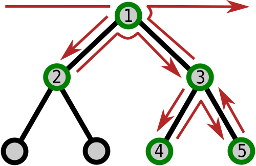
Figure 21: Stages of a two-stage filter applied to one constituting hypertree within a binary hypertree grid. Left: pre-processing stage with post-order DFS traversal, using a lightweight cursor, selecting vertices check-marked in green. Right: main stage with pre-order DFS traversal with a heavier cursor, only across pre-selected vertices. The indices reflect the order in which vertices are processed by each stage.

In order to circumvent this difficulty, we devised a two-pass approach where a more lightweight cursor is used to traverse the entire mesh in a pre-processing stage, selecting only those cells that are concerned by the algorithm. The dual-based computation is thus only performed in the subsequent processing stage, where only those pre-selected parts of the grid are actually traversed by the most expensive Moore supercursor. Specifically and as illustrated in Figure 21, the pre-selection stage uses post-order DFS traversal, in order to propagate upwards per-branch selection (and possibly aggregated attribute information as well), whereas the main stage is performed with pre-order DFS fashion, immediately processing the pre-selected cells in the order in which they are reached when skipping non-selected branches. Albeit more complex in appearance, this two-stage approach can in fact be dramatically more efficient than a direct traversal of the input grid with the most complex cursor, provided a clever pre-selection criterion not requiring neighborhood information be contrived. The key success factor to this approach thus rests on devising a criterion that is easy to compute with minimal information and yet is discriminatory enough so as to avoid as many false positives as possible (while false negatives will result in an incomplete output).

4.6.3 Concrete Filters

We now provide a brief overview of the filters we have developed so far, as concrete instances of our cursor-based general methodology. This list can, and most likely will, be extended as dictated by tree-based AMR post-processing needs.

AxisCut:

produce a $2$-dimensional hypertree grid output from a $3$-dimensional input, comprising the intersection of all cells in the latter that are intercepted by an axis-aligned plane. The output has an associated material mask only when the input has one.

AxisClip:

clip, i.e., mask out all input cells that do not fulfill a geometric condition that can take three forms: hyperplane, rectangular prism (shorthand box), or quadratic function. In hyperplane mode, only those leaf cells that are either intersected by said hyperplane or wholly within a prescribed half-space that it defines are retained. A similar selection process occurs in box mode, based on whether cells are intersected by said box or located entirely in its interior. In quadratic mode, a leaf cell is retained if and only if said function takes on positive values at all corners of this cell. The hypertree grid output always has a material mask even when the input does not.

AxisReflection:

already presented as a geometric transformation filter exemplar in §4.6.1.

CellCenters:

generate the set of points consisting of the centers of the leaf cells in a hypertree grid, with the option to make it also a polygonal data set containing only vertex elements.

Contour:

compute polygonal data sets representing iso-contours corresponding to a set of given values for the cell-wise attribute, using a dual-based approach with a pre-selection criterion discussed in detail in §4.7.

DepthLimiter:

stop the descent into each of the constituting hypertrees whenever either a leaf or the requested maximum depth are reached; in the latter case, a leaf is issued to replace the reached node, and therefore all its descendants too. The output is a hypertree grid that has a material mask only if the input does as well.

Dual:

generate the entire dual mesh, possibly adjusted. For the reasons developed in §3.5, this filter should never be used with sizable hypertree grid inputs, but only for prototyping or illustration purposes.

Geometry:

generate the outside surface of a hypertree grid as a polygonal data set, in particular for rendering purposes. Note that, already memory costly in dimension $3$, this conversion into an unstructured mesh can, in dimension $2$, create an output whose footprint is orders of magnitude larger than that of the hypertree grid input.

PlaneCutter:

similar to the AxisCut, except that it can take an arbitrary plane as cut function, to produce a polygonal data set output. This filter has two modes of operation: primal or dual. In primal mode, both topology and geometry of the original leaf cells are preserved, hereby ensuring that no interpolation error occur and that the cut planes extend to the primal boundary, at the topological cost of producing T-junctions wherever the cut plane intercepts an interface between cells at different depths.

Threshold:

produce a hypertree grid output with an associated material mask, even when the input does not have any, in order to mark out all cells whose attribute value is not within a specified range.

ToUnstructured:

generate a fully explicit unstructured grid data set whose elements are exactly the leaf cells of the input hypertree grid, represented as rectangular prisms (i.e., lines, quads, or voxels depending on the dimensionality of the input). The output thus has exactly the same geometric support as the input; it is not a conforming mesh due to the presence of T-junctions. It is also prohibitively expensive for sizable AMR meshes and shall thus only be used for prototyping or illustration purposes.

Table 1: Cursors vs. filters: unless otherwise mentioned, check-marks correspond to the cursors used to iterate over the input grid, when needed (which is not always the case). $d$ denotes the dimensionality of the input grid. Cursors are arranged left to right in increasing order of complexity. ^∗Note that for the Dual filter, old “simple” super-cursor was sufficient because no neighbor geometry information is necessary as dual points are all computed and stored explicitly.

	TreeCursor	TreeGridCursor	GeometricCursor	VonNeumannSuperCursor	MooreSuperCursor
AxisClip	✓(output)		✓
AxisCut	✓(output)		✓
AxisReflection
CellCenters			✓
Contour		✓(pre-processing)			✓
DepthLimiter	✓(output)	✓
Dual					✓∗
Geometry			✓($d<3$)	✓($d=3$)
PlaneCutter primal dual		✓(pre-processing)	✓		✓
Threshold	✓(output)	✓
ToUnstructuredGrid			✓

These filters are implemented using their respective minimal cursors within the set described in §3.6. The correspondence between filters and cursors is provided in Table 1; it is left to the reader to examine why these relationships are indeed both correct and minimal.

4.7 Iso-Contouring

We conclude this methodological discussion by emphasizing the case of iso-contouring, because it is arguably one of the most widely used amongst all existing visualization techniques, while being especially difficult to perform on AMR grids – in practice, impossible when dealing with large grids if they must be converted to an explicit grid prior to iso-contouring. It is important to mention that we iso-contour hypertree grid attribute fields by considering only their values at leaf nodes. This design choice is made in order to simplify a complex problem. Note however that subsequent implementations could be allowed to take into account field values at strict tree nodes as well. That said, there is no known, efficient iso-contouring algorithm for general polyhedral meshes. Instead, the canonical approach is to subdivide polyhedra into simplices which are subsequently iso-contoured. As discussed in §3, this approach is prohibitive in terms of memory footprint and execution time. It is therefore natural to consider a dual-based approach to tackle iso-contouring of hypertree grids. Therefore, as explained in §4.6.2, the computational efficiency of the algorithm rests upon an astute pre-selection criterion to decide whether a cell may be intercepted by an iso-contour without any information retrieval concerning its neighbors.

Given a hypertree grid $\mathcal{H}$ with $n_{v}$ vertices and an array $C$ of iso-values, our selection criterion defines $\lvert{C}\lvert$ Boolean arrays with length $n_{v}$ called sign arrays. For every value in $C$ with index $j\in\llbracket\lvert{C}\lvert\llbracket$, the corresponding signed array is denoted $S_{j}$. The goal of each $S_{i}$ is to capture the relative position of the field of interest at all tree vertices, with True (resp. False) when the cell-centered value is greater (resp. smaller) than $C[j]$. We also define another Boolean array, $T$, called the truth array, with length $n_{v}$ has well. $T$ is global to the entire set of iso-contours and is used to pre-select tree cells that will be immediately iso-contoured by the main processing phase. Only one such $T$ is used across all iso-contours because a dual cell must be generated when required by at least one iso-value.

Algorithm 3 $\mathtt{RecursivelyPreProcessTree}(c)$

1:  $i\leftarrow\mathtt{GetGlobalIndex}(c)$

2:  $T[i]\leftarrow$False

3:  if $\mathtt{IsLeaf}(c)$ then

4:     for all $j\in\llbracket\lvert\mathcal{C}\lvert\llbracket$ do

5:        $S_{j}[c]\leftarrow(\texttt{GetAttributeValue}(c)>\mathcal{C}[j])$

6:     end for

7:  else

8:     for all $j\in\mathcal{\llbracket}{f^{d}}\llbracket$ do

9:        $c^{\prime}\leftarrow\mathtt{GetChild}(c,j)$

10:        $T[i]\overset{\lor}{\leftarrow}\mathtt{RecursivelyPreProcessTree}(c^{\prime})$

11:        if $\neg T[i]$ then

12:           $k\leftarrow\mathtt{GetGlobalIndex}(c^{\prime})$

13:           for all $l\in\llbracket\lvert\mathcal{C}\lvert\llbracket$ do

14:              if $\neg{j}$ then

15:                 $S_{l}[i]\leftarrow S_{l}[k]$

16:              else

17:                 if $\neg(S_{l}[i]\oplus S_{l}[k])$ then

18:                    $T[i]\leftarrow\texttt{True}$

19:                 end if

20:              end if

21:           end for

22:        end if

23:     end for

24:  end if

25:  return  $T[i]$

Algorithm 3 summarizes the pre-processing stage, for every cursor position $c$ inside the input hypertree grid $\mathcal{H}$. The goal of this function is two-fold: first, store the position of the attribute value of $c$ relative to each of the iso-values in each of the $S_{i}$ arrays; second, store the truth value at $T[c]$ to indicate whether $c$ is intercepted by at least one iso-contour. When $c$ is coarse, $T[c]$ can be True only when $c$ has in its descent at least two leaf cells with opposed signs; in this case, the $S_{i}[c]$ values are irrelevant. In contrast, when $c$ is coarse and $T[c]$ is False, then its entire descent has the same sign, defining the value stored in $S_{i}[c]$; in this case, $T[c]$ as well as the $S_{i}[c]$ values are relevant. When $c$ is a leaf, $T[c]$ is not meaningful and is assigned False by default; in this case, the $S_{i}[c]$ values are relevant. As required, Algorithm 3 needs neither geometric nor topological information, hereby allowing for the use of the lightweight TreeGridCursor for the pre-processing stage.

Algorithm 4 $\mathtt{RecursivelyProcessTree}(s)$

1:  if $\mathtt{IsLeaf}(s)$ then

2:     if $\neg\mathtt{Masked}(s)$ then

3:        for all $i\in\llbracket 2^{d}\llbracket$ do

4:           if $\mathtt{IsOwner}(s,i)$ then

5:              $D\leftarrow\mathtt{GenerateDualCell}(s,i)$

6:              for all $j\in\llbracket\lvert\mathcal{C}\lvert\llbracket$ do

7:                 $\mathcal{I}\,\overset{+}{\leftarrow}\mathtt{MarchingCube}(D,j)$

8:              end for

9:           end if

10:        end for

11:     end if

12:  else

13:     $i\leftarrow\mathtt{GetGlobalIndex}(s)$

14:     for all $j\in\llbracket\lvert\mathcal{C}\lvert\llbracket$ do

15:        for all $k\in\mathcal{\llbracket}{2^{d}}\llbracket$ do

16:           $l\leftarrow\mathtt{GetNeighborGlobalIndex}(s,k)$

17:           if $T[i]\lor T[l]\lor S_{j}[i]\neq S_{j}[l]$ then

18:              for all $k\in\mathcal{\llbracket}{f^{d}}\llbracket$ do

19:                 $\mathtt{RecursivelyProcessTree}(\mathtt{GetChild}(s,k))$

20:              end for

21:              return  

22:           end if

23:        end for

24:     end for

25:  end if

Subsequently, the contouring stage executes the function RecursivelyProcessTree(), described in Algorithm 4, upon every cell of $\mathcal{H}$, using a Moore supercursor $s$. For each generated dual cell $D$ and each contour value $\mathcal{C}[j]$, the call to $\mathtt{MarchingCube}(D,\mathcal{C}[j])$ returns set of polygons (possibly empty) that is appended to the iso-contour mesh $\mathcal{I}$.

Figure 22: Close-up view of an iso-surface generated by the native Contour filter with a large hypertree grid input.

Figure 22 illustrates the results of the main iso-contouring phase, following the pre-processing stage, in the case of a large AMR simulation.

5 Results

We now discuss the main results obtained with the hypertree grid object, beginning with a study of its performance in terms of memory footprint. We continue with an overview of the filters that we have developed so far for this object. This section ends with a detailed analysis of the axis-aligned reflection filter, demonstrating the massive memory savings allowed for by our approach based on separating geometry from topology. These results are those obtained with our concrete implementation in VTK version 7.

5.1 Hypertree Grid Object

We begin with the case of a hypertree grid with $150$ constituting hypertrees, used to represent a variable number of cells in an AMR mesh.

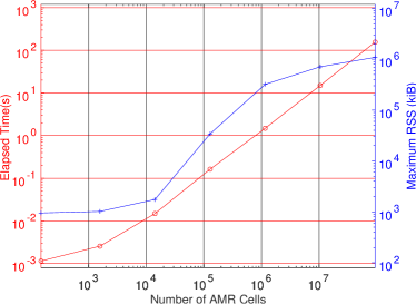
Figure 23: Execution time (red) and memory footprint (blue) versus number of cells in a synthetic hypertree grid.

Figure 23 illustrates this case, when a varying number of cells is obtained by increasing the tree depth $\delta\in[1;6]$. When $\delta=1$, only root-level cells are present in the constituting hypertrees, resulting in relatively high memory fixed costs per hypertree; as $\delta$ increase, these costs are progressively diluted by the ensuing greater number of hypertree cells. In addition, we observe a linear speedup in terms of execution time, hereby demonstrating the scalability of our approach.

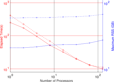
Figure 24: Execution time (red) and memory footprint (blue) versus number of processors used to represent a 2D AMR mesh with $\mathcal{O}(10^{8})$ leaves; solid (resp. dashed) lines correspond to a hypertree (resp. unstructured) grid.

Figure 24 demonstrates the strong scalability (i.e, with fixed total workload) of our approach, which scales almost optimally for memory footprint, and super-optimally for execution time, until maximum speedup is achieved for this problem size. Moreover, when comparing the performance in terms of memory footprint of our hypertree grid object with respect to that of using an unstructured grid representation, we note almost a full order of magnitude improvement (approximately a factor of $7$). Furthermore, we have observed that this massive decrease in memory usage remains constant across a wide range of workload distribution schemes for highly refined meshes.

5.2 Hypertree Grid Filters

We now illustrate some results obtained with the native hypertree grid filters presented in §4.6.3 and implemented in VTK, exploring the $2$ and $3$-dimensional cases as well as the two possible branch factor values.

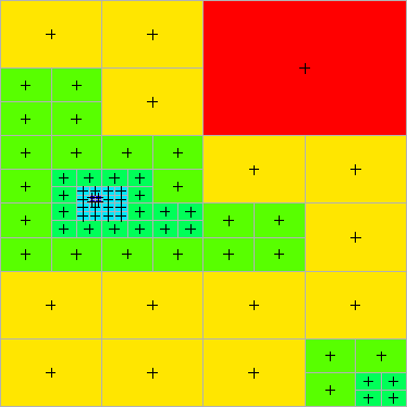
(a)

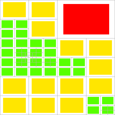
(d)

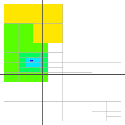
(g)

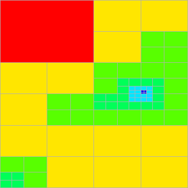
(b)

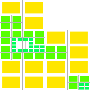
(e)

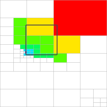
(h)

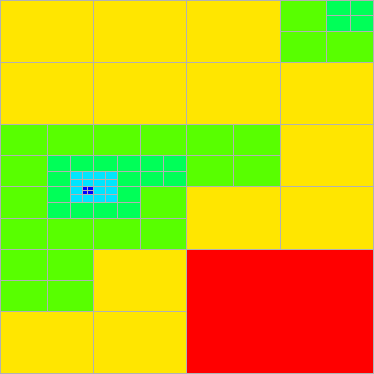
(c)

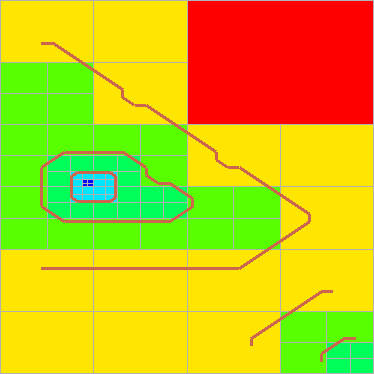
(f)

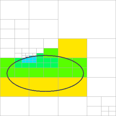
(i)

Figure 25: Visualizations of the data sets produced by application of native filters to a $2$-dimensional, binary hypertree grid with 6 root cells. In all of these, the Geometry filter was used in order to display the underlying AMR mesh, where colors represent cell depth used a cell-centered attribute: CellCenters (a), AxisReflection (b&c), respectively across vertical and horizontal center lines DepthLimiter (d) Threshold (e), Contour (f), AxisClip (g) through (i), respectively by 2 lines parallel to the grid axes, a axis-aligned rectangle, and an ellipse.

We begin with visualizations obtained when the input data set is a 2-dimensional binary hypertree grid, with a $2\times 3$ layout of root cells, to which is attached a single attribute field filled with the cell depths. Figure 25 applies the native hypertree grid Geometry filter (note that shrinkage of the output geometry is sometimes used in order to facilitate the interpretation of the results) to render hypertree grid outputs. In addition to it, these images illustrate the following filters:

(a)

CellCenters, hooked to a glyphing filter to produce the black crosses shown at cell centers.

(b&c)

AxisReflection, where hyperplanes are lines, respectively parallel to the vertical and horizontal axes, passing through the center of the hypertree grid.

(d)

DepthLimiter with depth limit is set to $2$.

(e)

Threshold for attribute values within $[1;3]$.

(f)

Contour with attribute iso-values $1.25$, $2.5$, and $3.75$. Note that, as explained in §3.5, the contours are topologically correct but do not intercept the primal boundary, because a non-adjusted dual is used.

(g–i)

AxisClip, illustrated for each of its three modes of operation, respectively: hyperplane (here, with 2 consecutive appelications), box, and a quadratic corresponding to an axis-aligned ellipse; note that alignment with the grid axes is not required by the filter as any arbitrary quadratic can be specified.

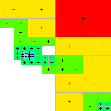
(a)

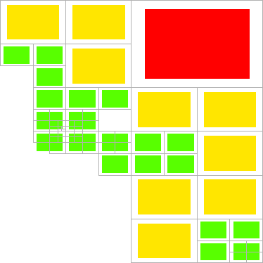
(d)

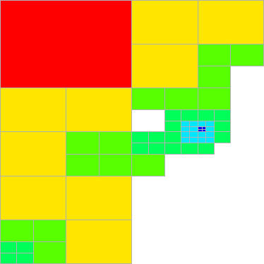
(b)

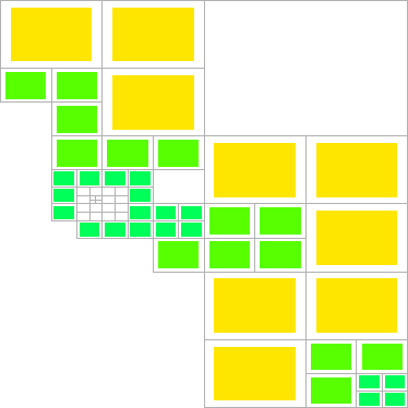
(e)

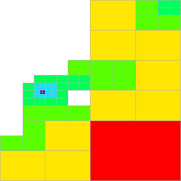
(c)

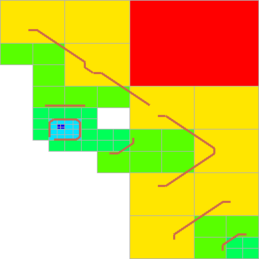
(f)

Figure 26: Results of the same tests as the first six shown Figure 25, but when a non-empty material mask was added to the input grid.

The results computed by the same filters, but when a non-empty material mask is attached to the hypertree grid input, are shown in Figure 26. We are not showing here the results obtained with the AxisClip filters in order to save space, but suffices to say that corresponding images are obtained are expected.

Of particular interest is the iso-contouring case (f): because the current implementation of the filter uses a non-adjusted dual, the computed iso-contours exhibit additional geometric oddities in the vicinity of the non-convexities resulting from the presence of masked cells. In our typical, large-scale applications, the phenomena of interest which are searched for in the post-processing stage tend to be removed from object boundaries (external or internal); therefore, geometric error in computed iso-contours are generally not encountered. It however remains our goal to provide the option to adjust the dual in future implementations.

The case of the DepthLimiter filter (d) also reveals an interesting feature, that can only present itself when non-convexities are present – and therefore, only when a non-empty mask is attached to the input hypertree grid. Specifically, the hypertree grid output by the filter can have a larger geometric extent that the input. This results from the fact that an input coarse cell at the depth limit is retained to create an output leaf as soon as at least one of its descendents is not masked. Indeed, this behavior can be observed in the figure, with the green cell at depth $2$ located at the middle-left of the grid.

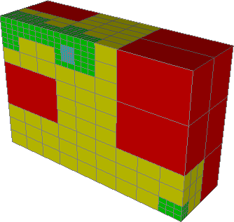
(a)

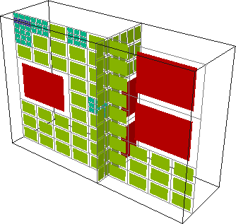
(d)

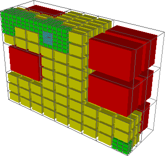
(g)

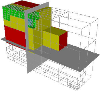
(j)

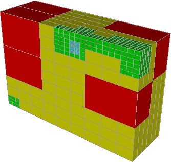
(b)

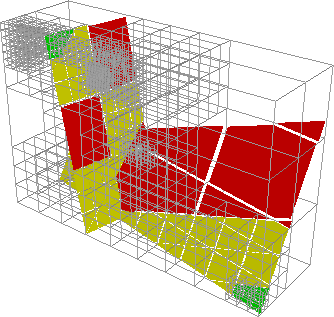
(e)

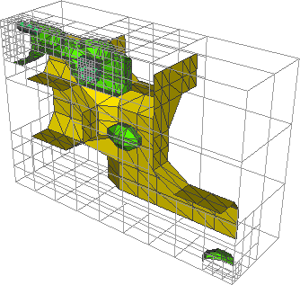
(h)

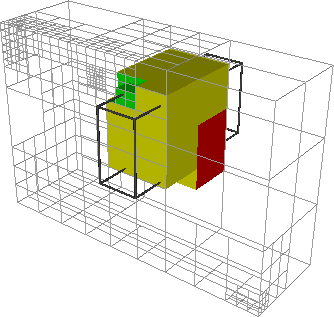
(k)

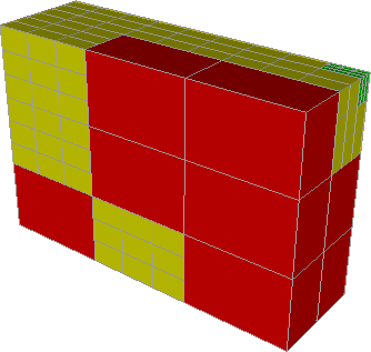
(c)

(f)

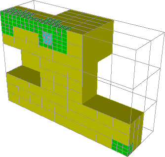
(i)

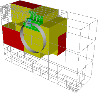
(l)

Figure 27: Renderings of the outputs of hypertree grid filters to a $3$-dimensional, ternary hypertree grid with 18 root cells. The hypertree grid Geometry filter was used to represent the input AMR mesh in wireframe mode wherever visible, as well as the output hypertree grid objects whenever applicable, where colors represent cell depth: Geometry (a), AxisReflection (b&c), respectively across one and two axis-aligned planes, AxisCut (d), PlaneCutter (e&f), respectively in primal and dual mode, ToUnstructured (g), Contour (h), Threshold (i), (j–l): AxisClip, respectively by 2 planes parallel to the grid axes, an axis-aligned box, and a cylinder.

A $3$-dimensional, ternary set of test cases is now used, with a $3\times 3\times 2$ layout of roots to further illustrate our point. In Figure 27, we show visualizations obtained with the following filters (note that Geometry is used to visualize all hypertree grid outputs):

(a)

Geometry.

(b&c)

AxisReflection, respectively with 1 and 2 successive reflections about planes passing through the center of the hypertree grid.

(d)

AxisCut with two axis-aligned cut planes, producing two $2$-dimensional hypertree grids, whose geometry is shrunk for legibility.

(e&f)

PlaneCutter which, in contrast, produces polygonal data sets, respectively in primal and dual modes. The main benefit of latter is its conforming mesh output, and it should thus always used when subsequent post-processing requiring perfect connectivity is intended; it is however important to note that is not only less visually appealing, but also considerably slower than the former.

(g)

ToUnstructured, whose all-hexahedral unstructured grid output is connected downstream to a shrink filter. As discussed in §2.1, the resulting unstructured mesh is not conforming, because interior faces are not shared but replicated.

(h)

Contour, again with three iso-values.

(i)

Threshold, for depth values within $[1;3]$.

(j–l)

AxisClip with its three modes of operation: respectively, two successive clips with planes parallel to the grid axes, an axis-aligned box, and a quadratic associated with a cylinder of revolution about the third coordinate axis.

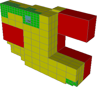
(a)

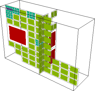
(d)

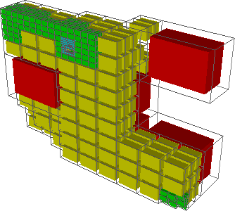
(g)

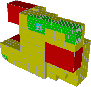
(b)

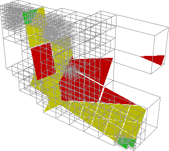
(e)

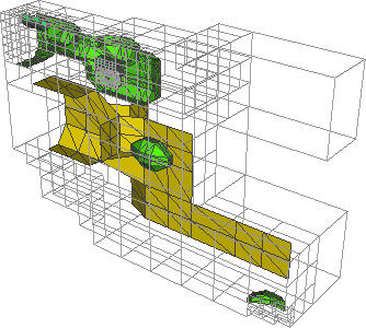
(h)

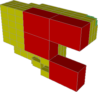
(c)

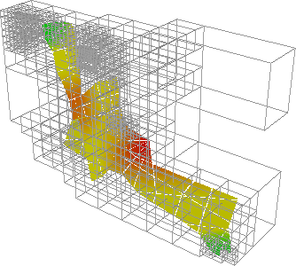
(f)

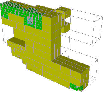
(i)

Figure 28: Results of the same tests as the first six shown Figure 27, but when a non-empty material mask was added to the input grid.

As previously done with the $2$-dimensional cases, Figure 28 present a subset of these cases, but obtained with a non-empty mask attached to the input hypertree grids. Comments similar to those made in the $2$-dimensional, binary case can be made and we will not therefore repeat ourselves. The interested reader is invited to draw parallels between corresponding $2$ and $3$ dimensional sub-figures, and to inspect the contents of the test harness we implemented for all existing hypertree grid filters, across different dimensions, branching factors, and other modalities: to date, 58 individual tests are available and can be either executed as they are, or modified and experimented with at will.

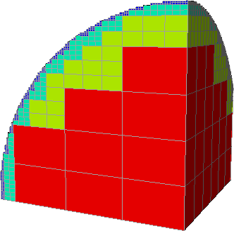
Figure 29: Left: the first octant of a truncated unit ball, approximated with 5 levels of a ternary tree-based AMR grid with $5\times 5\times 6$ root cells. Right: a rendering showing the same truncated octant (upper right corner), together with its successive images (in solid colors) by axis-aligned reflections, yielding a truncated unit ball.

We close this discussion with the particular case of the AxisReflection filter. In Figure 29, we illustrate the use of this filter by applying it to the case of a ternary tree-based AMR grid with $5\times 5\times 6$ root cells, where a material mask is defined using a quadratic function retaining only those cells that are within or intersect a truncated octant of the unit ball. The experiment thus consisted in creating this object, hereafter referred to as the octant, then performing seven reflection across planes, adequately defined in order to produce outputs whose union, together with the initial octant, produces the unit ball truncated by the original plane and its symmetrical about the sphere center. This output is referred to as the reflections. Octant creation, geometry extraction and rendering times were excluded from this experiment in order to assess the performance of the AxisReflection filter in isolation.

Table 2: Main characteristics, and memory footprints in terms of maximum resident set size, of a ternary hypertree grid object (octant), its $8$-time replication (octant*8) and of its union (reflections) with 7 images thereof by the AxisReflection filter.

	Number	Number	Number	RSS
	of cells	of leaves	of trees	(kiB)
octant	$128724$	$123962$	$150$	44924
octant*8	$1029792$	$991696$	$1200$	359392
reflections	$1029792$	$991696$	$1200$	45172

The main results of this experiment performed on a single core are summarized in Table 2; in particular, the reflections represents an AMR mesh 8 times larger, with over one million cells (96.3% of which are leaf cells), than the original octant. Executing the 7 reflections took a negligible time, compared to the octant creation or its rendering, hereby confirming the theoretical prediction that, if correctly implemented, the reflection filter should have negligible execution time. Another key finding of this test was to measure a negligible increase in memory readings, as compared to the real replication of the object requiring a commensurate increase in memory footprint (which might not be available to the target platform). These results demonstrate that our implementation fully delivers the promises of the theoretical analysis, in terms of execution speed as well as of memory footprint. As a result, all future hypertree grid structure-preserving geometry transformation filters shall be implemented following the same paradigm.

6 Conclusion

There are many more details to this story than we could possibly fit within the frame of a journal article. What are we, then, to make of this already long exposé, which encompassed general motivations, theoretical foundations, application methods, and experimental results?

In the next few lines, we will first look back on what has been achieved so far, as compared to what we were initially envisioning. This will allow us to conclude with a set of remarks as to our subsequent projects and goals, articulating them within our general vision together with what we have discovered and done during the course of the work described in this article.

6.1 Main Findings

We set out in §2.2 ([a]) with the goal to propose a novel VTK data object that would be able to support all conceivable types of rectilinear, tree-based AMR data sets, based not only on today’s software but also on what we can foresee of tomorrow’s extreme-scale simulations. We can confidently claim that we have accomplished this first goal, based on the vtkHyperTreeGrid object and its family of lesser objects presented throughout this article. In particular, the key design constraint to drastically reduce memory usage, as compared to either earlier implementations of this object or to different, existing VTK data objects, was fully achieved. This was amply demonstrated by our numerical results in in §5, consistent with what the theory laid out in  §3 was allowing to hope for. This achievevement dramatically reduces hardware requirements by several orders of magnitude, as compared to the alternatives currently used in AMR visualization.

Moreover, we propounded in §2.2 ([b]) to design and implement visualization filters that could natively operate on this novel data object, with the added stated goal of measurable performance in terms of execution speed. We have also entirely fulfilled our objectives in this regard, with demonstrated performance improvements with respect to our earlier design and implementation (not to mention the alternatives which are plainly useless for large-scale meshes).

Meanwhile, in the process of designing such filters, we entirely revised our earlier notion of tree cursors and, more importantly, supercursors. This resulted, in particular, in the introduction of a hierarchy of such objects in order to allow for the selection of the cursor that is the most tightly adapted to the particular algorithm being considered. Due in particular to use of templates, as well to the careful nesting of geometric and topological cursor properties, this results in the added benefits of enhanced code maintainability and legibility. This new incarnation of the hypertree grid object allows us to confidently assert that it can be used even by an application developer not intimately familiar with the implementation details.

An other important aspect of this work is the availability of a full set of visualization filters able to natively operate over the novel data object. As explained this article, these filters have all been written with performance in mind, in terms of both memory footprint and execution speed. Furthermore, our design based on the hierarchy of templated cursors and supercursors, combined with the pre-selection paradigm for enhanced performance, gives developers the opportunity to easily create new filters tailored to their particular needs.

After all has been said in terms of theoretical soundness, or of convincing experimental results, what is ultimately our main claim to success is that our HERA code users at CEA have been able to begin routine post-processing of their AMR simulations, within a setting similar to that which already exists for the visualization of simulations based on other types of meshes.

Based on these findings, we decided to contribute our development to the VTK code base so it can benefit the tree-based AMR community at large.

6.2 Perspectives

As formulated in §2.2, we have considered many potential avenues for further advances in the field of tree-based AMR visualization and analysis. These are not only of academic interest; in fact, they appear as strictly necessary when considering the post-processing options that are commonly available for other types of simulations, such as the finite element method using fully unstructured, conforming meshes.

First, we expecte that our original goal [b] will be further achieved, as the community of users of our contributed code will increase and expand to connected yet different application domains.

Meanwhile, 2-dimensional AMR visualization can be especially challenging, as it requires that all leaf cells be rendered. In consequence, the interactivity of the visualization process decreases as input data object size increases. This problem is further compounded by the enhanced efficiency, in terms of memory footprint, of our hypertree grid model which elicits a new situation where rendering has become the bottleneck for our the target platforms. As a result, the next goal ([c]) is indeed an urgent need, for which the lack of existing solution is currently hindering the AMR visualization and analysis workflow. Our preliminary developments in this regard should be finalized, validated and contributed shortly. These focus on rendering speed, in particular in dimension 2, by exploiting level-of-detail properties, which we also plan to carefully study and explain in a sequel to this article.

Besides, the $3$-dimensional visualization technique known as volume rendering, which has now been broadly used for almost two decades, for different types of data objects, remains mostly unchartered territory when it comes to tree-based AMR data and would come in direct support of our stated goal ([d]). Iso-contouring is often derided as being the “poor man’s volume rendering”. Albeit excessive, as in many cases an iso-surface is exactly what is required by the nature of the analysis being performed, this statement nonetheless usefully conveys the general idea that “true” 3-dimensional visualization is a capability that most if not all users want to have in a visualization tool set before they deem it sufficient. Considerable theoretical and experimental effort will be required in order to support this need, for almost no prior work exists in this area. However, such a major endeavor could potentially be amortized by 2-dimension specializations in addition to the overarching 3-dimensional goal.

The work done so far does not address per se any of items [e]-[g] in our initial vision. However, we believe that the theoretical groundwork which we have already conducted will allow for an easier pursuit of these goals in the future.

Last, we would like to close this panorama by mentioning an ongoing reflection regarding in situ and in transit visualization and analysis. This contemplates the possibilities that exist to directly couple an existing production-level AMR simulation code with a visualization tool set adapted to it, in a fashion that would entirely eliminate intermediate storage to disk. We are confident that this will allow us to address the last vision item ([h]) in the near future, which will be discussed in subsequent work.

Acknowledgments

This work was supported by the French Alternative Energies and Energy Atomic Commission (CEA) for Military Applications (DAM). We are grateful for advice from C. Guilbaud and N. Lardjane (CEA) and helpful discussions with J.-C. Frament (Positiveyes). We also thank D. Chapon at the Institute of Research into the Fundamental Laws of the Universe (Irfu) for providing RAMSES large-scale simulation results and helping us exploit these to generate the astrophysics-related visualization results shown in this article. This article could not have been written without the support and patience of ours families.

References

- [1] CEA’s Tera supercomputer. http://www-hpc.cea.fr/en/complexe/tera.htm.
- [2] Overview of block structured AMR. Online: https://commons.lbl.gov/display/chombo/ Overview+of+Block+Structured+AMR.
- [3] Patch-based adaptive mesh refinement for multimaterial hydrodynamics. In Joint Russian-American Five-Laboratory Conference on Computational Mathematics/Physics, Vienna, Austria, June 2005.
- [4] D. Aguilera, T. Carrard, G. Colin de Verdière, J.-P. Nominé, and V. Tabourin. Parallel software and hardware for capability visualization of HPC results. Numerical Modeling of Space Plasma Flows: Astronum, 2007.
- [5] D. Aguilera, T. Carrard, C. Guilbaud, J. Schneider, and S. Sorbet. Visualization and post-processing for high performance computing. CHOCS, 41:57–67, 2012.
- [6] L. Avila, U. Ayachit, S. Barré, J. Baumes, F. Bertel, R. Blue, D. Cole, D. DeMarle, B. Geveci, W. Hoffman, B. King, K. Krishnan, C. Law, K. Martin, W. McLendon, P. Pébay, N. Russell, W. Schroeder, T Shead, J. Shepherd, A. Wilson, and B. Wylie. The VTK User’s Guide. Kitware, Inc., eleventh edition, 2010.
- [7] D. Bale, R. J. LeVeque, S. Mitran, and J. A. Rossmanith. A wave-propagation method for conservation laws and balance laws with spatially varying flux functions. SIAM J. Sci. Comput., 24:955–978, 2002.
- [8] M. J. Berger, D. L. George, R. J. LeVeque, and K. T. Mandli. The GeoClaw software for depth-averaged flows with adaptive refinement. Adv. Water Res., 34:1195–1206, 2011.
- [9] M. J. Berger and J. Oliger. Adaptive mesh refinement for hyperbolic partial differential equations. J. Comput. Phys., 53(3):484–512, 1984.
- [10] A. Bondy and U.S.R. Murty. Graph Theory. Graduate Texts in Mathematics. Springer London, 2011.
- [11] O. Bressand, L. Colombet, A. Fontaine, G. Harel, and J.-B. Lekien. Hercule: A library of scientific data management for numerical simulation. CHOCS, 41:29–37, 2012.
- [12] T. Carrard, C. Law, and P. Pébaÿ. A generic hyper tree grid implementation for AMR mesh manipulation and visualization in VTK. In Proc. 21st International Meshing Roundtable, San Jose, CA, U.S.A., October 2012.
- [13] B. Delaunay. Sur la sphère vide. Bul. Acad. Sci. URSS, Class. Sci. Nat., pages 793–800, 1934.
- [14] P. Frey and P.-L. George. Mesh generation. John Wiley & Sons, 2 edition, 2008.
- [15] B. Fryxell, K. Olson, P. Ricker, F. X. Timmes, M. Zingale, D. Q. Lamb, P. MacNeice, R. Rosner, J. W. Truran, and H. Tufo. FLASH: An adaptive mesh hydrodynamics code for modeling astrophysical thermonuclear flashes. The Astrophysical Journal Supplement Series, 131(1):273, 2000.
- [16] M. Gittings, R. Weaver, M. Clover, T. Betlach, N. Byrne, R. Coker, E. Dendy, R. Hueckstaedt, K. New, W. R. Oakes, D. Ranta, and R. Stefan. The RAGE radiation-hydrodynamic code. Computational Science & Discovery, 1(1), 2008.
- [17] H. Jourdren. HERA: A hydrodynamic AMR platform for multi-physics simulations. In Adaptive Mesh Refinement Theory and Application, volume 41 of LNCSE, pages 283–294. Springer, 2005.
- [18] N. Packard and S. Wolfram. Two dimensional cell automata. J. Comput. Phys., (38):901–946, 1985.
- [19] R. Teyssier. Cosmological hydrodynamics with adaptive mesh refinement. a new high resolution code called RAMSES. Astronomy and Astrophysics, 385:337–364, 2002.
- [20] P. Woodward, J. Jayayaraj, P.H. Lin, Mike M. Knox, D. Porter, C. Fryer, G. Dimonte, C. Joggerst, G. Rockefeller, W. Dai, R. Kares, and V. Thomas. Simulating turbulent mixing from Richtmyer-Meshkov and Rayleigh-Taylor instabilities in converging geometries using moving cartesian grids. Technical Report LA-UR-13-20949, Los Alamos National Laboratory, 2012.
- [21] M.-M. Yau and S. N. Srihari. A hierarchical data structure for multidimensional digital images. Communications of the ACM, 26(7):504–515, July 1983.