Off-shell gluon production in interaction of a projectile with 2 or 3 targets

Abstract

Within the effective QCD action for the Regge kinematics amplitudes for virtual gluon emission are studied in collision of a projectile with two and three targets. It is demonstrated that all un-Feynman singularities cancel between induced vertices and rescattering contributions. Formulas simplify considerably in a special gauge which is a straightforward generalization of the light-cone gauge for emission of real gluons.

1 Introduction

In the framework of the perturbative QCD at high energies and in Regge kinematics strong interactions can be described in terms of reggeized gluons (”reggeons”), which combine into colorless pomerons exchanged between colliding hadrons. Reggeons and their interactions were first introduced in the dispersion approach, using multiple unitarity cuts  [1, 2]. Later, mostly to describe next order contributions, a convenient and powerful method of effective action was proposed in which the reggeons figure as independent dynamical fields interacting with the standard gluons  [3].The effective action allows to present scattering amplitudes in the Regge kinematics as a sum of diagrams, similar to the Feynman ones with certain rules for propagators and interaction vertices  [4]. The latter, apart from the standard QCD vertices, include the so-called induced vertices in which the reggeons interact with two or more gluons. In the effective action approach the scattering amplitudes depend not only on the transversal variables but also on the longitudinal ones. So one has to perform the longitudinal integrations to reduce the result to the purely transverse form, as in the dispersion approach mentioned above. In applications to the amplitudes with many in-coming or out-going reggeons these integrations are not trivial, since the induced vertices contain singularities in longitudinal variables different from the standard Feynman ones. In earlier papers  [5, 6] it was shown however that amplitudes for emission of a real gluon in transition of a reggeon into two or three reggeons in fact can be rewritten in the purely transverse form with the standard transversal vertices connected with Feynman propagators. The contribution from induced vertices becomes substituted by the one from the Feynman propagators of the rescattering projectile. This result greatly simplifies application of the approach to real processes, as was illustrated in  [7] where scattering off the deuteron projectile was studied. Note that this result heavily rested on the use of a specific gauge, in which the gluon polarization vectors were chosen to be orthogonal to the target momentum and in which the relevant vertices radically simplify.

However in applications (say for the total cross-sections) also vertices for production of a virtual gluon appear. So the question arises whether the same conclusion holds also in this case. Concretely if also for the virtual gluon production the contribution from the induced vertices can be traded for the contribution from the projectile rescattering, thereby liquidating non-Feynman singularities introduced by induced vertices and reducing longitudinal integration to the standard Feynman ones. This problem is the aim of the present study. We shall find that the answer is positive in the sense that the un-Feynman poles are canceled between the contributions from the vertex and rescattering. There also exists a special gauge in which the bulk of the result is reduced to essentially transverse vertices connected by Feynman propagators. However this also requires certain small change in the transverse vertices and taking a new polarization into account.

These conclusions are rather straightforward in the transition into two out-going reggeons, considered in Sections 2 and 3. A considerably more complicated case of three out-going reggeons is studied in Sections 4 and 5. Our conclusions are presented in Section 6.

Note that in  [8, 9] some simple processes initiated by virtual gluons and essentially mediated by a single reggeon exhchange were studied. Validity of the effective action technique was confirmed. However reggeon splitting was not considered, so that the problems treated in our paper were not encountered.

2 Emission of a virtual gluon in interaction with two targets

The amplitude for production of a gluon with momentum $p$, polarization vector $e_{\mu}$ and color $c$ in the transition of a reggeon into two reggeons with momenta $q_{1}$ and $q_{2}$ and colors $b_{1}$ and $b_{2}$ is represented by three diagrams shown on Fig. 1. The left diagram corresponds to emission from the effective vertex $V$ for transition of a reggeon to two reggeons plus the virtual gluon (R$\to$RRP vertex). The other two correspond to rescattering of the projectile.

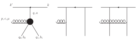
Figure 1: Production amplitude: vertex and rescattering contributions

2.1 Emission from the vertex $V$

The amplitude corresponding to the left diagram in Fig 1 is given by

$${\cal A}^{V}={\cal A}^{V}_{\mu}e^{\mu},\ \ {\cal A}^{V}_{\mu}=g^{3}\bar{u}(k^{\prime})\gamma^{+}u(k)f^{ab_{1}d}f^{db_{2}c}T^{a}\frac{1}{q_{\perp}^{2}}V_{\mu}.$$

Here $k$ and $k^{\prime}$ are the initial and final 4-momenta of the projectile; $q=p+q_{1}+q_{2}$, $q_{-}=0$. We suppress factors coming from the targets, which have their initial 4-momenta $l$. In the c.m. system both $k$ and $l$ have zero transverse components and $k_{-}=l_{+}=0$. $T$ is the quark color matrix. The R$\to$RRP vertex is $V=V_{1}+\Big{(}1\leftrightarrow 2\Big{)}$. In the general gauge and for arbitrary $p$ part $V_{1}$ is given by

$$V_{1\mu}=\frac{i}{4}\Big{\{}\frac{a_{\mu}}{d_{1}}+\frac{b_{\mu}}{q_{1-}d_{1}}+\frac{c_{\mu}}{q_{1-}}\Big{\}},$$ (1)

where $d_{1}$ is the Feynman denominator $d_{1}=(q-q_{1})^{2}+i0$,

$$a(p,q_{2},q_{1})=p_{+}(3p+4q_{1}+4q_{2})\mu-2p_{+}^{2}n_{\mu}^{-}$$

$$+n_{\mu}^{+}\Big{(}-(p+2q_{1}+q_{2},p-q_{2})+q_{1}^{2}+q_{2}^{2}-(p+q_{1}+q_{2})^{2}-(p+q_{2})^{2}+2p_{+}p_{-}\Big{)},$$ (2)

$$b(p,q_{2},q_{1})=-2(p+q_{1}+q_{2})^{2}_{\perp}\Big{[}(p+2q_{2})_{\mu}-p_{+}n_{\mu}^{-}+n_{\mu}^{+}\Big{(}\frac{q_{2}^{2}}{p_{+}}+p_{-}\Big{)}\Big{]}$$ (3)

and

$$c=2n_{\mu}^{-}\frac{(p+q_{1}+q_{2})_{\perp}^{2}}{p_{-}}.$$ (4)

Here $n^{\pm}=(1,0,0,\mp 1)$. Note that $Vp=0$ for arbitrary $p$. Terms in (1) contain poles of the Feynman type at $(q-q_{1})^{2}=0$ and un-Feynman type at $q_{1-}=0$ coming from the induced vertices. To separate the latter we use

$$\frac{1}{q_{1-}d_{1}}=\frac{q_{+}}{(q-q_{1})_{\perp}^{2}d_{1}}+\frac{1}{q_{1-}(q-q_{1})_{\perp}^{2}}.$$ (5)

Then $V_{1}$ is transformed into two parts

$$V_{1}=\frac{i}{4}\Big{\{}\frac{1}{d_{1}}\Big{(}a+\frac{p_{+}b}{(q-q_{1})_{\perp}^{2}}\Big{)}+\frac{1}{q_{1-}}\Big{(}\frac{b}{(q-q_{1})_{\perp}^{2}}+c\Big{)}\Big{\}}.$$ (6)

We introduce the generalized off-mass-shell Lipatov vertex

$$2L_{\mu}(p,q_{2})=-\frac{1}{(p+q_{2})_{\perp}^{2}}\Big{\{}(p+2q_{2})_{\mu}+\Big{(}\frac{q_{2}^{2}}{p_{+}}+p_{-}\Big{)}n^{+}_{\mu}-\Big{(}\frac{(p+q_{2})_{\perp}^{2}}{p_{-}}+p_{+}\Big{)}n^{-}_{\mu}\Big{\}}.$$ (7)

It goes into the standard Lipatov vertex when $p_{-}+q_{2-}=0$, so that $p_{-}=-q_{2-}$. However we preserve this definition also for $p_{-}+q_{2-}\neq 0$, as in our case when $p_{-}+q_{2_{-}}=-q_{1-}$. With this definition we find

$$\frac{b}{(q-q_{1})_{\perp}^{2}}+c=4(p+q_{1}+q_{2})^{2}L(p,q_{2}).$$ (8)

The first term in (6) may be used as the definition of the off-mass-shell Bartels vertex

$$a+\frac{p_{+}b}{(q-q_{1})_{\perp}^{2}}=-4p_{+}(p+q_{1}+q_{2})^{2}B(p,q_{2},q_{1}).$$ (9)

so that the vertex $V$ as a whole can be rewritten in the same form as on the mass shell in the gauge $(el)=0$  [5]

$$V_{1}=i(p+q_{1}+q_{2})^{2}\Big{\{}-\frac{p_{+}B(p,q_{2},q_{1})}{(p+q_{2})^{2}+i0}+\frac{L(p,q_{2})}{q_{1-}}\Big{\}}.$$ (10)

as well as the amplitude corresponding to emission from the vertex

$${\cal A}^{V}=ig^{3}\bar{u}(k^{\prime})\gamma^{+}u(k)f^{ab_{1}d}f^{db_{2}c}t^{a}\Big{[}-\frac{p_{+}B(p,q_{2},q_{1})}{(p+q_{2})^{2}+i0}+\frac{L(p,q_{2})}{q_{1-}}\Big{]}+\Big{(}1\leftrightarrow 2\Big{)}.$$ (11)

Here the unwanted un-Feynman pole at $q_{1-}=0$ is separated in the second term.

For a real emitted gluon the un-Feynman poles in $V$ were canceled by the contribution from the rescattering diagrams on the right in Fig. 1. Presently we study if this also happens with the virtual emitted gluon.

2.2 Emission from rescattering

The two diagrams in Fig. 1 on the right describe emission of a gluon during rescattering of the projectile. If one takes into account the full Feynman projectile propagator they give in the sum

$${\cal A}^{RF}=\frac{g^{3}\bar{u}(k^{\prime})\gamma^{+}u(k)}{q_{2-}+i0}L(p,q_{1})f^{b_{1}cd}t^{b_{2}}t^{d}+\frac{g^{3}\bar{u}(k^{\prime})\gamma^{+}u(k)}{-q_{1-}+i0}L(p,q_{2})f^{b_{2}cd}t^{d}t^{b_{1}}+\Big{(}1\leftrightarrow 2\Big{)}.$$ (12)

Emission vertex $L(p,q_{1})$ is the Lipatov vertex (7) for of-mass-shell gluon. Note that in contrast to (7) here the sum of ”-” components of the two arguments is equal to zero. However, with our definition in which only $p_{-}$ is used, these Lipatov vertices coincide with those in (11).

The propagators can be split into the principal value and delta function terms

$$\frac{1}{\pm q_{1,2-}+i0}={\cal P}\frac{1}{\pm q_{1,2-}}-i\pi\delta(q_{1,2-}).$$

As was discussed in  [5], in the contribution from rescattering one has to keep only the part of the projectile propagator containing the $\delta$-function. The part containing the principal value should be dropped. So the final rescattering contribution is

$${\cal A}^{R}=g^{3}\bar{u}(k^{\prime})\gamma^{+}u(k)\left[-i\pi\delta(q_{2-})L(p,q_{1})f^{b_{1}cd}\Big{\{}t^{b_{2}},t^{d}\Big{\}}-i\pi\delta(q_{1-})L(p,q_{2})f^{b_{2}cd}\Big{\{}t^{d},t^{b_{1}}\Big{\}}\right].$$ (13)

Expression (12) With Feynman propagators is given by the sum

$${\cal A}^{RF}={\cal A}^{R}+{\cal A}^{RP},$$ (14)

where ${\cal A}^{RP}$ contains contributions from the principal value parts of the propagators. One finds

$${\cal A}^{RP}=ig^{3}\bar{u}(k^{\prime})\gamma^{+}u(k)f^{ab_{1}d}f^{db_{2}c}t^{a}{\cal P}\frac{1}{q_{1-}}L(p,q_{1})+\Big{(}1\leftrightarrow 2\Big{)}$$ (15)

It coincides with the second part of (11) containing the Lipatov vertices, provided the singularities at $q_{1.2-}=0$ are taken in the principal value sense. In the sum of the vertex and rescattering contributions according to (14) this second part restores the Feynman propagators in the latter thereby canceling all un-Feynman singularities in the total amplitude, which becomes

$${\cal A}^{tot}=-ig^{3}\bar{u}(k^{\prime})\gamma^{+}u(k)f^{ab_{1}d}f^{db_{2}c}T^{a}\frac{p_{+}B(p,q_{2},q_{1})}{(p+q_{2})^{2}+i0}+{\cal A}^{RF}.$$ (16)

So in the end the amplitude does not contain any singularities different from those provided by the standard Feynman propagators either for the intermediate gluon or for the rescattering quark.

The final expression for the amplitude is rather complicated. However, as for the real emitted gluon, it drastically simplifies by the choice of a suitable gauge.

3 Quasi-lightcone gauge

Off-mass shell gluons have 3 instead of 2 polarizations. It is possible to choose polarization vectors with a minimal difference as compared to real gluons. One can choose two of them (transversal) in the same manner as on the mass shell imposing condition $(e^{T}l)=0$ where $l$ is the target momentum. Then

$$e^{T}_{+}=0,\ \ e^{T}_{-}=-\frac{(e^{T}p)_{\perp}}{p_{+}},\ \ \Big{(}e^{T}\Big{)}^{2}=-1.$$ (17)

The third, longitudinal in the 4-dimensional sense, can be chosen as

$$e^{L}_{\mu}=\frac{\sqrt{p^{2}}}{p_{+}}n^{+}_{\mu}-\frac{1}{\sqrt{p^{2}}}p_{\mu}$$ (18)

with the properties

$$(e^{L}p)=(e^{T}e^{L})=0,\ \ \Big{(}e^{L}\Big{)}^{2}=-1.$$ (19)

Vectors $e^{T}$, $e^{L}$ together with vector $e^{(0)}_{\mu}=p_{\mu}/\sqrt{p^{2}}$ form a set of 4 independent orthonormalized vectors in the Lopenz space in which any polarization vector can be expanded. Excluding $e^{(0)}$ for spin 1 particle one can use $e^{T}$ and $e^{L}$ as polarization vectors. We call this gauge quasi-lightcone, having in mind that the purely transverse polarizations are the same as for the real gluon.

In addition to our previous products with transverse polarizations we have then to add products with $e^{(L)}$. Due to orthogonality of vertices to $p$ this is equivalent to additional products with $n^{+}$. Since $(e^{T}n^{+})=\Big{(}n^{+}\Big{)}^{2}=0$ all terms in the amplitude proportional to $n^{+}$ vanish in this gauge. So in the end we can drop all terms in the vertex containing $p_{\mu}$ or $n_{\mu}^{+}$. This drastically simplifies the resulting expressions.

Effectively this means that in this gauge we can take

$$a_{\mu}=4p_{+}(q_{1}+q_{2})_{\mu}-2p_{+}^{2}n_{\mu}^{-},\ \ b_{\mu}=-2q^{2}(2q_{2\mu}-p_{+}n_{\mu}^{-}).$$ (20)

First we study contribution from polarization $e^{T}$. One finds

$$(ae^{T})=4p_{+}(qe^{T})_{\perp},\ \ (be^{T})=-4q^{2}(p+q_{2},e^{T})_{\perp},\ \ (ce^{T})=-4q^{2}\frac{(pe^{T})_{\perp}}{p_{+}p_{-}}.$$

As a result we get from (9)

$$(Be^{T})=\frac{(p+q_{2},e^{T})_{\perp}}{(p+q_{2})^{2}_{\perp}}-\frac{(p+q_{1}+q_{2},e^{T})_{\perp}}{(p+q_{1}+q_{2})^{2}_{\perp}}.$$ (21)

This is the same expression which one had for the on-mass-shell gluon. So in this quasi-lightcone gauge, the contribution from the transverse polarizations does not feel the off-mass-shellness of the gluon. On the other hand we get

$$\Big{(}Le^{T}\Big{)}=\frac{(pe^{T})_{\perp}}{p_{\perp}^{2}-p^{2}}-\frac{(q-q_{1},e^{T})_{\perp}}{(q-q_{1})_{\perp}^{2}}.$$ (22)

Comparing with the real gluon we find a change $p_{\perp}^{2}\to p_{\perp}^{2}-p^{2}$ in the denominator.

So for polarizations $e^{T}$ the changes in the amplitude (16) are minimal: part from the vertex $V$ does not change at all and in the rescattering part the Lipatov vertex contains $p_{\perp}^{2}-p^{2}$ instead of simply $p_{\perp}^{2}$.

The new parts come from polarization $e^{L}$. One finds

$$(an^{+})=-4p_{+}^{2},\ \ (bn^{+})=4q^{2}p_{+},\ \ (cn^{+})=4\frac{q^{2}}{p_{-}}.$$

This gives

$$(Be^{L})=\sqrt{p^{2}}\Big{(}\frac{1}{q^{2}}-\frac{1}{(p+q_{2})_{\perp}^{2}}\Big{)}$$ (23)

and for the rescattering

$$(Le^{L}\Big{)}=\sqrt{p^{2}}\Big{(}\frac{1}{(p+q_{2})_{\perp}^{2}}-\frac{1}{p_{\perp}^{2}-p^{2}}\Big{)}.$$ (24)

This ends the study of the scattering on two centers. We have found that, first, as for the real emitted gluon all un-Feynman singularities at $q_{1,2}=0$ actually go when one uses full Feynman propagators for rescattering. Second, in the specially chosen gauge results for the purely transversal polarizations are nearly identical with the real gluon case (except for the addition of $-p^{2}$ to $p_{\perp}^{2}$ in the denominators of the Lipatov emission vertices for rescattering). New contributions from polarization $e^{L}$ are proportional to $\sqrt{p^{2}}$ and also contain the additional $-p^{2}$ in the Lipatov vertices. Apart from this they do not depend on longitudinal variables.

4 Interaction with three targets. The R$\to$RRRP vertex.

In addition to $d_{1}=(q-q_{1})^{2}+i0$ we introduce $d_{2}=(q-q_{1}-q_{2})^{2}+i0$. Here $q=p+q_{1}+q_{2}+q_{3}$. We shall use (5) and and

$$\frac{1}{d_{2}(q_{1-}+q_{2-})}=\frac{q_{+}}{(q-q_{1}-q_{2})^{2}_{\bot}d_{2}}+\frac{1}{(q-q_{1}-q_{2})^{2}_{\bot}}\frac{1}{q_{1-}+q_{2-}}$$ (25)

The amplitude for the gluon emission from the R$\to$RRRP in interaction of the projectile with three targets is illustrated in Fig. 2. The vertex is composed of various contributions diagrammatically shown in Fig. 3. The numbers of diagrams in the following refer to this figure. Black disks refer to effective vertices in Lipatov’s effective action. Discs with cross indicate the so-called induced vertices. The dot in diagram 2 corresponds to the QCD 4-gluon coupling.

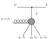
Figure 2: The amplitude with the R$\to$RRRP vertex.

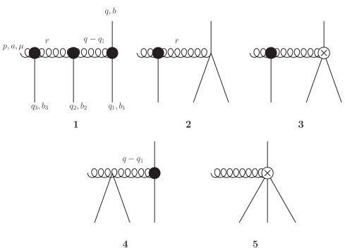
Figure 3: Diagrams for the R$\to$RRRP vertex.

4.1 Diagram 1

We separate the common factor

$$F_{1}=\frac{1}{8}\frac{g^{4}}{q^{2}}\bar{u}(k^{\prime})\gamma_{+}u(k)f^{b_{3}ad}f^{b_{2}dc}f^{bb_{1}c}t^{b}$$ (26)

The expression for the diagram can then be written as

$$D_{1}=-\frac{A_{1}}{d_{1}d_{2}}-\frac{B_{1}}{q_{1-}d_{1}d_{2}}.$$ (27)

Here

$$A_{1}=p_{+}^{2}(8q-p)_{\mu}-4p_{+}^{3}n_{\mu}^{-}+p_{+}n_{\mu}^{+}\Big{[}(q_{2}+q_{3}-3p)(q+q_{1})$$

$$+q_{2}^{2}+2q_{3}^{2}+q_{1}^{2}+q^{2}-p^{2}-(p-q_{3},p+2q_{2}+q_{3})+4p_{+}p_{-}\Big{]}$$ (28)

and

$$B_{1}=q^{2}\Big{\{}2p_{+}(-2r-4q_{2}-p-2q_{3})_{\mu}+4p_{+}^{2}n_{\mu}^{-}$$

$$+n_{\mu}^{+}\Big{[}-4p_{+}4p_{-}+6p^{2}-2(p-q_{2}-q_{3})^{2}-2(q-q_{1}-q_{2})^{2}\Big{]}\Big{\}}.$$ (29)

Using (5) we get

$$D_{1}=-\frac{1}{d_{1}d_{2}}\Big{(}A_{1}+\frac{q_{+}B_{1}}{(q-q_{1})_{\perp}^{2}}\Big{)}-\frac{B_{1}}{q_{1-}(q-q_{1})^{2}_{\perp}d_{2}}$$ (30)

Note that both $A_{1}$ and $B_{1}$ contain terms proportional to $(q-q_{1}-q_{2})^{2}$ which cancel one of the denominators.

4.2 Diagrams 2 and 3

For diagrams 2 and 3 we have

$$D_{2+3}=\frac{1}{d_{2}}\left(\frac{4p_{+}q_{\bot}^{2}n_{\mu}^{-}}{(q_{1}+q_{2})_{-}q_{1-}}-\frac{4q_{\bot}^{2}(p+2q_{3})_{\mu}}{(q_{1}+q_{2})_{-}q_{1-}}-\frac{2(p-q_{3})_{-}q_{\bot}^{2}n_{\mu}^{+}}{(q_{1}+q_{2})_{-}q_{1-}}-\frac{4q_{3}^{2}q_{\bot}^{2}n_{\mu}^{+}}{p_{+}(q_{1}+q_{2})_{-}q_{1-}}+2p_{+}n_{\mu}^{+}\right).$$ (31)

We use $q_{3-}=-(p+q_{1}+q_{2})_{-}$. Then we find three types of terms:

$$D_{2+3}=\frac{A_{2}}{d_{2}}+\frac{B_{2}}{q_{1-}d_{2}}+\frac{C_{2}}{q_{1-}(q_{1-}+q_{2-})d_{2}},$$ (32)

where

$$A_{2}=2p_{+}n_{\mu}^{+},\ \ B_{2}=-2q^{2}n_{\mu}^{+},$$

$$C_{2}=q^{2}_{\perp}\Big{\{}-4(p+2q_{3})_{\mu}+n_{\mu}^{+}\Big{(}-4p_{-}-4\frac{q_{3}^{2}}{p_{+}}\Big{)}+4p_{+}n_{\mu}^{-}\Big{\}}.$$ (33)

Using (25) we get

$$D_{2+3}=\frac{A_{2}}{d_{2}}+\frac{1}{q_{1-}d_{2}}\Big{(}B_{2}+\frac{q_{+}C_{2}}{(q-q_{1}-q_{2})_{\perp}^{2}}\Big{)}+\frac{C_{2}}{q_{1-}(q_{1}+q_{2})_{-}(q-q_{1}-q_{2})_{\perp}^{2}}$$ (34)

4.3 Diagram 4

Diagram 4 is

$$D_{4}=\frac{1}{d_{1}}\left(p_{+}n_{\mu}^{+}-\frac{2q_{\bot}^{2}n_{\mu}^{+}}{q_{1-}}.\right)$$ (35)

It contains two types of terms

$$D_{4}=\frac{A_{4}}{d_{1}}+\frac{B_{4}}{q_{1-}d_{1}},$$ (36)

where

$$A_{4}=p_{+}n_{\mu}^{+},\ \ B_{4}=-2q^{2}n_{\mu}^{+}.$$ (37)

Applying (5) we get

$$D_{4}=\frac{1}{d_{1}}\Big{(}A_{4}+\frac{q_{+}B_{4}}{(q-q_{1})_{\perp}^{2}}\Big{)}+\frac{B_{4}}{q_{1-}(q-q_{1})_{\perp}^{2}}.$$ (38)

4.4 Diagram 5

The diagram 5 is proportional to $1/[q_{1-}(q_{1-}+q_{2-})]$

$$D_{5}=\frac{B_{5}}{q_{1-}(q_{1}+q_{2})_{-}},\ \ B_{5}=4n_{\mu}^{-}\frac{q^{2}}{p_{-}}.$$ (39)

4.5 Total result

The total amplitude ${\cal A}^{V}$ coming from the vertex splits into three parts which we denote similarly to the on-mass shell case

$${\cal A}^{V}=g^{4}\bar{u}(k^{\prime})\gamma_{+}u(k)f^{b_{3}ad}f^{b_{2}dc}f^{bb_{1}c}t^{b}(W_{I}+Q_{I}+R_{I})\equiv{\cal A}^{VW}+{\cal A}^{VQ}+{\cal A}^{VR}$$ (40)

Here $W_{I}$ contains only the Feynman propagators whereas $Q_{I}$ and $R_{I}$ also contain un-Feynmam poles. The Feynman part is

$$W_{I}=\frac{1}{8q^{2}d_{1}d_{2}}\Big{(}-A_{1}-\frac{q_{+}B_{1}}{(q-q_{1})_{\perp}^{2}}\Big{)}+\frac{A_{2}}{8q^{2}d_{2}}+\frac{1}{8q^{2}d_{1}}\Big{(}A_{4}+\frac{q_{+}B_{4}}{(q-q_{1})_{\perp}^{2}}\Big{)}.$$ (41)

The part $Q_{I}$ contains terms with a pole at $q_{1-}=0$

$$Q_{I}=\frac{1}{8q^{2}q_{1-}d_{2}}\Big{\{}-\frac{B_{1}}{(q-q_{1})_{\perp}^{2}}+\frac{q_{+}C_{2}}{(q-q_{1}-q_{2})_{\perp}^{2}}+B_{2}\Big{\}}+\frac{B_{4}}{8q^{2}q_{1-}(q-q_{1})_{\perp}^{2}}.$$ (42)

Explicitly

$$Q_{I}=\frac{T_{1}+T_{2}+T_{3}}{q_{1-}d_{2}},$$ (43)

where

$$T_{1}=\frac{1}{8(q-q_{1})_{\perp}^{2}}\Big{\{}p_{+}(6p+8q_{3}+8q_{2})_{\mu}-4p_{+}^{2}n_{\mu}^{-}+n_{\mu}^{+}\Big{(}4p_{+}p_{-}-6p^{2}+2(p-q_{2}-q_{3})^{2}\Big{)}\Big{\}}$$ (44)

$$T_{2}=\frac{1}{8(q-q_{1}-q_{2})_{\perp}^{2}}\Big{\{}-4p_{+}(2q_{3}+p)_{\mu}+4p_{+}^{2}n_{\mu}^{-}-4n_{\mu}^{+}(p_{+}p_{-}+q_{3}^{2})\Big{\}}$$ (45)

$$T_{3}=-\frac{1}{4}n_{\mu}^{+}$$ (46)

$R_{I}$ contains terms proportional to $1/[q_{1-}(q_{1-}+q_{2-})]$:

$$R_{I}=\frac{1}{8q^{2}q_{1-}(q_{1-}+q_{2-})}\Big{(}\frac{C_{2}}{(q-q_{1}-q_{2})_{\perp}^{2}}+4n_{\mu}^{-}\frac{q^{2}}{p_{-}}\Big{)}$$

Explicitly

$$R_{I}=\frac{1}{q_{1-}(q_{1-}+q_{2-})}\,\frac{1}{8q^{2}(q-q_{1}-q_{2})^{2}_{\bot}}\Big{\{}-(p+2q_{3})_{\mu}-n_{\mu}^{+}\Big{(}p_{-}+\frac{q_{3}^{2}}{p_{+}}\Big{)}+n_{\mu}^{-}\Big{(}p_{+}+\frac{(p+q_{3})^{2}_{\perp}}{p_{-}}\Big{)}\Big{\}}$$

$$=\frac{1}{q_{1-}(q_{1-}+q_{2-})}L(p,q_{3}),$$ (47)

where we used our definition (7) of the generalized Lipatov vertex. To these contribution one also has to add 5 other terms with simultaneous permutations of momenta $q_{1,2,3}$ and color indices $b_{1,2,3}$ of the outgoing reggeons.

To finally sum all different contributions in Section 6 it will be convenient to present the color factor in the form

$$t^{b}f^{bb_{1}c}f^{cb_{2}d}f^{db_{3}a}=\frac{1}{i}[t^{b_{1}},t^{c}]f^{cb_{2}d}f^{db_{3}a}=-[t^{b_{1}},[t^{b_{2}},t^{d}]]f^{db_{3}a}$$

$$=(t^{b_{2}}t^{d}t^{b_{1}}+t^{b_{1}}t^{d}t^{b_{2}}-t^{d}t^{b_{2}}t^{b_{1}}-t^{b_{1}}t^{b_{2}}t^{d})f^{db_{3}a}.$$ (48)

4.6 Relation to the vertex R$\to$RRP

On the mass shell and in the gauge $(el)=0$ the vertex R$\to$RRRP could be related to the vertex R$\to$RRP. In fact we had then

$$W_{I}=\frac{p_{+}^{2}B(p,q_{2}+q_{3},q_{1})}{[(q-q_{1})^{2}+i0][(q-q_{1}-q_{2})^{2}+i0]},$$ (49)

$$Q_{I}=-\frac{p_{+}B(p,q_{3},q_{2})}{q_{1-}[(q-q_{1}-q_{2})^{2}+i0]}$$ (50)

and

$$R_{I}=\frac{L(p,q_{3})}{q_{1-}(q_{1-}+q_{2-})}$$ (51)

where $B$ and $L$ were the standard Bartels and Lipatov vertices. The cancelation of all un-Feynman singularities heavily relied on the relations (50) and (51).

As we have found relation (51) indeed holds also for the off-mass-shell gluon and in the arbitrary gauge. So our central problem is to see if (50) is also valid for the off-shell gluon in the arbitrary gauge.

From our study of the R$\to$RRP vertex we determined (in fact defined) the generalized Bartels vertex $B$ by Eq. (9). It follows that

$$-p_{+}B(p,q_{3},q_{2})=\frac{1}{4(p+q_{2}+q_{3})_{\perp}^{2}}\Big{(}a(p,q_{3},q_{2})+\frac{p_{+}b(p,q_{2},q_{3})}{2(p+q_{3})_{\perp}^{2}}\Big{)}.$$ (52)

In fact we have seen that

$$p_{+}b=-2p_{+}(p+q_{2}+q_{3})_{\perp}^{2}\beta,$$

where

$$\beta=(p+2q_{3})_{\mu}-p_{+}n_{\mu}^{-}+n_{\mu}^{+}\Big{(}\frac{q_{3}^{2}}{p_{+}}+p_{-}\Big{)}.$$

So we get

$$-p_{+}B(p,q_{3},q_{2})=\frac{a}{4(p+q_{2}+q_{3})_{\perp}^{2}}-\frac{p_{+}\beta}{2(p+q_{3})^{2}}.$$ (53)

It contains two terms with different singularities in the transverse space. Our expression for $Q_{I}$ also has two terms with the same singularities plus a term with no singularities whatsoever, which can be included in any of the two previous ones with the appropriate factor.

Forgetting this factor for a while have therefore to compare $T_{1}$ with $a/(p+q_{2}+q_{3})_{\perp}^{2}$ and $T_{2}$ with $b/(p+q_{3})_{\perp}^{2}$ We start from $T_{2}$. Presenting

$$T_{2}=\frac{t_{2}}{8(p+q_{3})_{\perp}^{2}}$$

we have

$$t_{2}=-4\Big{(}p_{+}(p+2q_{3})_{\mu}-p_{+}^{2}n_{\mu}^{-}+n_{\mu}^{+}(p_{+}p_{-}+q_{3}^{2}\Big{)}$$

to be compared with the second term in (53). We find that they are identical, so that the part containing $1/(p+q_{3})_{\perp}^{2}$ in $Q_{I}$ has indeed the form (50).

Now we compare terms containing $1/(p+p_{2}+p_{3})_{\perp}^{2}$ We present

$$T_{1}+T_{3}=\frac{t_{1}}{8(p+q_{2}+q_{3})_{\perp}^{2}},$$

where from our previous calculations

$$t_{1}=2p_{+}(3p+4q_{2}+4q_{3})_{\mu}-4p_{+}^{2}n_{\mu}^{-}+n_{\mu}^{+}\Big{(}4p_{+}p_{-}-6p^{3}+2(p-q_{2}-q_{3})^{2}-2(p+q_{2}+q_{3})_{\perp}^{2}\Big{)}.$$ (54)

Taking into account factor $1/8$ and $1/4$ in $p_{+}B$, $t_{1}$ is to be compared with

$$2a(p,q_{3},q_{2})=2p_{+}(3p+4q_{2}+4q_{3})_{\mu}-4p_{+}^{2}n_{\mu}^{-}$$

$$+2n_{\mu}^{+}\Big{(}-(p+2q_{2}+q_{3},p-q_{3})+q_{2}^{2}+q_{3}^{2}-(p+q_{2}+q_{3})^{2}_{\perp}-(p+q_{3})^{2}+2p_{+}p_{-}\Big{)}.$$ (55)

We observe that the first two terms are identical. The coefficients before $n_{\mu}^{+}$ are: in $t_{1}$

$$-6p^{2}+2(p-q_{2}-q_{3})^{2}-2(p+q_{2}+q_{3})_{\perp}^{2}+4p_{+}p_{-}$$

and in $2a$

$$-2(p+2q_{2}+q_{3},p-q_{3})+2q_{2}^{2}+2q_{3}^{2}-(p+q_{3})^{2}-2(p+q_{2}+q_{3})^{2}_{\perp}+4p_{+}p_{-}$$

The last two terms are identical. The first ones give in $t_{1}$

$$-4p^{2}+2q_{2}^{2}+2q_{3}^{2}-4pq_{2}-4pq_{3}+4q_{2}q_{3}$$

and in $2a$

$$-2p^{2}-4pq_{2}-2pq_{3}+2pq_{3}+4q_{2}q_{3}+2q_{3}^{2}+2q_{2}^{2}+2q_{3}^{2}-2p^{2}-2q_{3}^{2}-4pq^{3}$$

These two expressions also coincide.

So we have proven that (50) is also true for the emission of a virtual gluon in an arbitrary gauge. This opens the way to demonstrate that all un-Feynman singularities in ${\cal A}^{V}$ are canceled by the rescattering contributions, provided one takes full Feynman quark propagators in them and treats appropriately the singularities at $q_{i-}=0$ and $q_{i-}+q_{k-}=0$ with $i\neq k=1,2,3$.

As to relation (49)inspection of our results shows that it does not hold generally. However in the quasi-lightcone gauge it is fulfilled indeed. In fact in that gauge, as mentioned, we can drop all terms with $p_{\mu}$ and $n_{\mu}^{+}$. Then one finds

$$A_{1\mu}=8p_{+}(q_{1}+q_{2}+q_{3})_{\mu}-4p_{+}^{2}n_{\mu}^{-},\ \ B_{1\mu}=4q_{2}\Big{(}2(q_{2}+q_{3})_{\mu}-2p_{+}n_{\mu}^{-}\Big{)}.$$ (56)

Comparison with (20) shows that this corresponds to changing $q_{2}\to q_{2}+q_{3}$ from which (49) indeed follows in the quasi-lightcone gauge.

5 Rescattering

In the rescattering the gluon is emitted by vertices R$\to$RRP and R$\to$RP (Lipatov) which are known for off-mass-shell emitted gluon. The diagrams themselves are quite obvious and do not differ from the on-mass-shell case. So for calculating the rescattering contribution we can use our results derived for on-mass-shell emission in  [6] substituting for the Bartels and Lipatov vertices their expression for the off-mass-shell gluon and in the arbitrary gauge introduced in our Section 2. Some details of the manipulations with color factors can also be found in  [6].

5.1 Single rescattering. Diagrams in Fig. 4

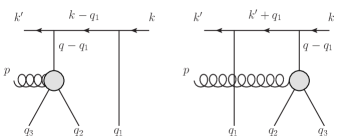
Figure 4: Diagrams with the double interaction of the projectile and the gluon emitted from the R$\to$RRP vertex.

Diagrams with a single rescattering of the projectile separate into two groups with emission of the gluon from the R$\to$RRP vertex shown in Fig. 4 and from a reggeon shown in Fig. 5.

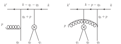
Figure 5: Diagrams with the double interactions of the projectile and the gluon emitted from the R$\to$RP vertex.

In both diagrams grey disks correspond to the R$\to$RRP vertex given analytically in (10). Since the vertex is symmetrical with respect to permutation of the two outgoing reggeons, the symmetrization for diagrams in Fig. 4 has to be carried out only for cyclic permutations of reggeons 1,2,3. The color factors are

$$C_{1}=-if^{db_{3}a}(T^{b_{2}}T^{d}T^{b_{1}}-T^{d}T^{b_{2}}T^{b_{1}})$$ (57)

for the first diagram and

$$C_{2}=-if^{db_{3}a}(T^{b_{1}}T^{b_{2}}T^{d}-T^{b_{1}}T^{d}T^{b_{2}})$$ (58)

for the second one.

The projectile factors, apart from the color factors, contain the quark propagators, which in the Regge limit are

$$\frac{1}{\pm q_{1-}+i0}$$ (59)

with the sign ”-” for the left diagram and ”+” for the right one. As mentioned in the rescattering only the delta-function part of the propagator should be left. So (59) should be substituted as

$$\frac{1}{\pm q_{1-}+i0}\to-i\pi\delta(q_{1-}).$$ (60)

With these preliminaries we find the contribution to the rescattering amplitude from Fig. 4 as

$${\cal A}^{R}_{1}=g^{4}\bar{u}(k^{\prime})\gamma_{+}u(k)(C_{1}+C_{2})(-i\pi)\delta(q_{1-})\Big{[}-\frac{q_{+}B(p,q_{3},q_{2})}{(q-q_{1}-q_{2})^{2}+i0}+\frac{L(p,q_{3})}{q_{2-}}\Big{]}.$$ (61)

5.2 Single rescattering. Diagrams in Fig. (5)

Passing to the diagrams in Fig. 5 we have their color factors

$$C_{3}=-if^{db_{3}a}(T^{d}T^{b_{1}}t^{b_{2}}-T^{d}T^{b_{2}}T^{b_{1}})$$

for the first diagram and

$$C_{4}=-if^{db_{3}a}(T^{b_{1}}t^{b_{2}}T^{d}-T^{b_{2}}T^{b_{1}}T^{d})$$

for the second

The three-reggeon vertex R$\to$RR was calculated in [5], to be

$$\frac{gf^{cb_{1}b_{2}}}{2q_{1-}}(q_{1}+q_{2})_{\perp}^{2}=-\frac{gf^{cb_{1}b_{2}}}{2q_{2-}}(q_{1}+q_{2})_{\perp}^{2}$$ (62)

(we have $q_{1-}+q_{2-}=0$ in the vertex). The quark propagators are

$$\frac{1}{\pm(q_{1-}+q_{2-})+i0}$$

with signs ”-” for the first diagram and ”+” for the second. Taking into account that we have to leave only delta-functional parts we finally get the rescattering amplitude for Fig. 5 as

$${\cal A}^{R}_{2}=g^{4}\bar{u}(k^{\prime})\gamma_{+}u(k)(C_{3}+C_{4})(-i\pi)\delta(q_{1-}+q_{2-})\frac{L(p,q_{3})}{q_{1-}}+\Big{(}{\rm permutations}\ (123)\Big{)}$$ (63)

5.3 Double rescattering of the projectile

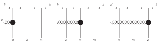
Figure 6: Diagrams with the triple interaction of the projectile.

There are 18 diagrams with three reggeons interacting with the projectile quark. Three of them are shown in Fig. 6, the others can be obtained by means of all permutations of reggeons 1,2,3. The color factors for the three diagrams in Fig. 6 are

$$C_{5}=f^{db_{3}a}T^{d}T^{b_{2}}T^{b_{1}},\ \ C_{6}=f^{db_{3}a}T^{b_{1}}T^{d}T^{b_{2}},\ \ C_{7}=f^{db_{3}a}T^{b_{2}}T^{b_{1}}T^{d}$$

The quark propagators are

$$\frac{1}{-(q_{1-}+q_{2-})+i0}\,\frac{1}{-q_{1-}+i0}$$

in the first diagram

$$\frac{1}{q_{1-}+i0}\,\frac{1}{-q_{2-}+i0}$$

in the second diagram and

$$\frac{1}{q_{1-}+i0}\,\frac{1}{q_{1-}+q_{2-}+i0}$$

in the third diagram. As it was discussed in  [5] due to locality in quark rapidity v.p. poles of quark propagators should be dropped. So in all propagators we are to retain only the $\delta$-functional parts. Taking into account that

$$\delta(q_{1-})\delta(q_{1-}+q_{2-})=\delta(q_{2-})\delta(q_{1}+q_{2-})=\delta(q_{1-})\delta(q_{2-})$$

we find the rescattering amplitude

$${\cal A}^{R}_{3}=-g^{4}\bar{u}(k^{\prime})\gamma_{+}u(k)L(p,q_{3})(C_{5}+C_{6}+C_{7})(-i\pi)^{2}\delta(q_{1-}\delta(q_{2-}).$$ (64)

6 Cancelation of un-Feynman singularities

Inspection of our expressions for the contributions from the R$\to$RRP vertex and from rescattering we see that they have exactly the same form as in the case of emitted on-mass-shell gluons in the gauge $(el)=0$. All the difference is due to the newly defined generalized Lipatov and Bartels vertices. The crucial point is that the same Bartels vertex $B(p,q_{3},q_{2})$ appears in the vertex amplitude ${\cal A}^{VQ}$ and rescattering amplitude ${\cal A}^{R}_{1}$, exactly as happens in the on-mass-shell case. As a result cancelation of un-Feynman singularities and restoration of Feynman propagators for the rescattering projectile proceeds in the same manner as in the on-mass-shell case  [6]. So we only briefly comment on the derivation.

Terms containing un-Feynman singularities separate into two groups depending on their momentum structure. One part contains the generalized Bartels vertex $B$. Contribution to this group come from the amplitude ${\cal A}^{VQ}$, Eq. (43), and the first term in the rescattering amplitude ${\cal A}^{R}_{1}$, Eq.(61). Taking into account (48) we find that these terms differ only in that factor $\pm 1/q_{1-}$ in ${\cal A}^{VQ}$ is substituted by $-i\pi\delta(q_{1-})$ in ${\cal A}^{R}_{1}$. In the sum of these two contributions we get the normal Feynman propagators

$$\pm\frac{1}{q_{1-}}-i\pi\delta(q_{1-})=\frac{1}{\pm q_{1-}+i0}.$$

As a result the contribution from $B(p,q_{3},q_{2})$ to the total amplitude will be given by

$${\cal A}^{VQF}_{1}g^{4}\bar{u}(k^{\prime})\gamma_{+}u(k)f^{b_{3}cd}\frac{q_{+}B(p,q_{3},q_{2})}{(q-q_{1}-q_{2})^{2}+i0}\Big{[}\frac{if^{ab_{2}d}T^{a}T^{b_{1}}}{-q_{1-}+i0}+\frac{if^{ab_{2}d}T^{b_{1}}T^{a}}{q_{1-}+i0}\Big{]},$$ (65)

which is actually the part of the rescattering contribution ${\cal A}^{R}_{1}$ with the Bartels vertex and Feynman propagator for the rescattering projectile.

Thus we are left with only the terms containing the Lipatov vertex $L$. They come from all contributions. We concentrate on the terms containing $L(p,q_{3})$. We separate the common factor

$$g^{4}\bar{u}(k^{\prime})\gamma_{+}u(k)f^{db_{3}a}L(p,q_{3}).$$

It has to be multiplied by the sum of different contributions from our amplitudes. Denoting different terms as $F^{I}$, $I=V,R1,R2,R3$ for contributions from amplitudes ${\cal A}^{VR}$, ${\cal A}^{R}_{1}$, ${\cal A}^{R}_{2}$ and ${\cal A}^{R}_{3}$ respectively we find

$$F^{VR}=\frac{T^{b_{2}}T^{d}T^{b_{1}}+T^{b_{1}}T^{d}T^{b_{2}}-T^{d}T^{b_{2}}T^{b_{1}}-T^{b_{1}}T^{b_{2}}T^{d}}{q_{1-}(q_{1-}+q_{2-})}+\Big{(}1\leftrightarrow 2\Big{)},$$

$$F^{R1}=-\frac{T^{b_{2}}T^{d}T^{b_{1}}-T^{d}T^{b_{2}}T^{b_{1}}+T^{b_{1}}T^{b_{2}}T^{d}-T^{b_{1}}T^{d}T^{b_{2}}}{q_{2-}}(-i\pi)\delta(q_{1-})+\Big{(}1\leftrightarrow 2\Big{)},$$

$$F^{R2}=\left(\frac{T^{d}T^{b_{2}}T^{b_{1}}}{q_{1-}}-\frac{T^{b_{2}}T^{b_{1}}T^{d}}{q_{2-}}\right)(-i\pi)\delta(q_{1-}+q_{2-})+\Big{(}1\leftrightarrow 2\Big{)},$$

$$F^{R3}=-(T^{d}T^{b_{2}}T^{b_{1}}+T^{b_{1}}T^{d}T^{b_{2}}+T^{b_{2}}T^{b_{1}}T^{d})(-i\pi)^{2}\delta(q_{1-})\delta(q_{2-})+\Big{(}1\leftrightarrow 2\Big{)}.$$ (66)

Straightforward algebraic manipulations (see  [6]) demonstrate that the sum of these contributions leads to the amplitude which corresponds to the double rescattering Fig. 4 with Feynman propagators for the rescattering projectile, namely

$${\cal A}^{RF}_{3}=-g^{4}\gamma_{+}f^{db_{3}a}\left[\frac{k_{+}^{2}\cdot T^{d}T^{b_{2}}T^{b_{1}}}{((k-q_{1}-q_{2})^{2}+i0)((k-q_{1})^{2}+i0)}+\frac{k_{+}^{2}\cdot T^{b_{1}}T^{d}T^{b_{2}}}{((k^{\prime}+q_{1})^{2}+i0)((k-q_{2})^{2}+i0)}\right.$$

$$+\left.\frac{k_{+}^{2}\cdot T^{b_{2}}T^{b_{1}}T^{d}}{((k^{\prime}+q_{2})^{2}+i0)((k^{\prime}+q_{1}+q_{2})^{2}+i0)}\right]L(p,q_{3})+\Big{(}\mbox{permutations of }1,2,3\Big{)}.$$ (67)

In conclusion the total amplitude for production of a virtual gluon on three centers is given by the sum of three contributions

$${\cal A}^{tot}={\cal A}^{VW}+{\cal A}^{VQF}+{\cal A}^{RF}_{3}$$ (68)

corresponding to emission from the vertex and single and double rescattering, in which all propagators are of the Feynman type.

In the general gauge this expression is quite complicated. However it drastically simplifies in the quasi-lightcone gauge, introduced in Section 3. For transverse polarizations the Bartels vertex takes its standard form and the Lipatov one only slightly changes. For longitudinal polarization both vertices become quite simple (Eqs. (23) and (24)).

6.1 Conclusion

We have found that with the gluon produced off mass shell both for two and three targets we can drop the induced part of the effective vertex and use instead full quark propagators in the rescattering contribution provided we interpret the singularities at $q_{1-}=0$ and $q_{2-}=0$ in the induced part in the principal value sense.

However in contrast to the on-mass-sell case the production amplitude cannot be deduced from the purely transverse BFKL-Bartels picture by just introducing Feynman propagators into the transverse Lipatov and Bartels vertices. Instead one has to appropriately change these vertices to account for the virtuality of the emitted gluon, so that they result to be not purely transversal.

A remarkably simple result follows in a particular gauge, which is an immediate generalization of the light-cone gauge for the off-mass-shell gluon. Then the changes in the vertices is minimal. Still a new, longitudinal, polarization is to be taken to account.

7 Acknowledgements

The authors acknowledge Saint-Petersburg State University for a research grant 11.38.223.2015 and RFFI for a research grant 15-02-02097A.

References

• [1] V.S.Fadin, E.A.Kuraev, L.N.Lipatov, Phys. Lett. B 60 (1975) 50; I.I.Balitsky, L.N.Lipatov, Sov. J. Nucl. Phys. 28 (1978) 822.
• [2] J.Bartels, Nucl. Phys. B 151 (1979) 293; Nucl. Phys. B 175 (1980) 365.
• [3] L.N.Lipatov, Nucl. Phys. B 452 (1995) 369: Phys. Rep. 286 (1997) 131.
• [4] E.N.Antonov, I.O.Cherednikov, E.A.Kuraev, L.N.Lipatov, Nucl. Phys. B 721 (2005) 111.
• [5] M.A.Braun, L.N.Lipatov, M.Yu.Salykin, M.I.Vyazovsky, Eur. Phys. J. C 71 (2011) 1639
• [6] M.A. Braun, M.Yu. Salykin, S.S. Pozdnyakov and M.I. Vyazovsky, Eur.Phys.J. C 72 (2012), N 11, 2223
• [7] M.A. Braun, M.Yu. Salykin, S.S. Pozdnyakov and M.I. Vyazovsky, Eur.Phys.J. C 73 (2013), N 9, 2572
• [8] A. van Hameren, P. Kotko, K.J. Kutak, High Energ. Phys. (2013) 2013: 78
• [9] A. van Hameren, K. Kutak, M. Serino, arXiv:1611.04380v3