Controlling competing orders via non-equilibrium acoustic phonons: emergence of anisotropic effective electronic temperature

Abstract

Ultrafast perturbations offer a unique tool to manipulate correlated systems due to their ability to promote transient behaviors with no equilibrium counterpart. A widely employed strategy is the excitation of coherent optical phonons, as they can cause significant changes in the electronic structure and interactions on short time scales. One of the issues, however, is the inevitable heating that accompanies these resonant excitations. Here, we explore a promising alternative route: the non-equilibrium excitation of acoustic phonons, which, due to their low excitation energies, generally lead to less heating. We demonstrate that driving acoustic phonons leads to the remarkable phenomenon of a momentum-dependent effective temperature, by which electronic states at different regions of the Fermi surface are subject to distinct local temperatures. Such an anisotropic effective electronic temperature can have a profound effect on the delicate balance between competing ordered states in unconventional superconductors, opening a novel avenue to control correlated phases.

I Introduction

One of the hallmarks of correlated electronic systems is the existence of multiple electronic orders with comparable energy scales that entangle different degrees of freedom. In the case of unconventional superconductors, such as iron pnictides, cuprates, and heavy fermions, superconductivity is usually found to compete with a density-wave type of order, characterized by a non-zero wave-vector $\mathbf{Q}$ Moon and Sachdev (2010). For instance, in the pnictides, $s^{+-}$ superconductivity competes with $\mathbf{Q}=\left(\pi,0\right)$ spin density-wave order Fernandes et al. (2010); in the cuprates, the $d$-wave superconducting transition temperature $T_{c}$ is suppressed by the onset of incommensurate charge order with ordering vector $\mathbf{Q}\approx\left(\frac{\pi}{3a},0\right)$ Chang et al. (2012); the superconducting state of the heavy fermions, on the other hand, competes with a Néel-type magnetic order, characterized by $\mathbf{Q}=\left(\pi,\pi\right)$ Pham et al. (2006). These observations open up the interesting possibility of enhancing superconductivity by suppressing the competing density-wave order.

The standard ways to experimentally tune the superconducting and density-wave orders in these materials is by chemical substitution, pressure, or magnetic field. Recent advances in ultrafast pump-and-probe techniques, however, opened a new avenue to explore and control these competing electronic states, as they generally undergo different relaxation processes to return to equilibrium Orenstein (2012); Giannetti et al. (2016); Rini et al. (2007); Fausti et al. (2011); Yang et al. (2014); Mankowsky et al. (2014); Vishik et al. (2016); Mitrano et al. (2016); Chia et al. (2010). Importantly, by taking the system out of equilibrium, its parameters change on ultrafast time scales, which can result in transient electronic states with no equilibrium counterpart. Indeed, an earlier experimental demonstration of non-equilibrium control of electronic order, based on pioneering ideas by Eliashberg Eliashberg (1960); Eliashberg and Ivlev (1986), was the surprising enhancement of superconductivity by sub-gap microwave irradiation Pals et al. (1982). More recently, ultrafast perturbations have been widely employed to manipulate unconventional superconductors by selecting particular lattice excitations of the system via optical pulses resonant with optical phonon modes Subedi et al. (2014). These coherent lattice excitations then modify the electronic structure and interactions of the system, which in turn can favor superconductivity or other electronic ordered states – a concept widely explored theoretically Fu et al. (2014); Moor et al. (2014); Dzero et al. (2015); Raines et al. (2015); Wang et al. (2016); Knap et al. (2016); Kennes et al. (2016); Kemper et al. (2016); Babadi et al. (2017). Examples include the melting of stripe order in the cuprates Fausti et al. (2011), the coherent modulation of the chemical potential in the pnictides Yang et al. (2014), and the possible promotion of transient superconductivity at high temperatures in organic superconductors Mitrano et al. (2016). There are however important issues intrinsic to this approach. First, the fact that the transient light-induced states only exist on ultrashort few picosecond time scales poses a key challenge to stabilize such non-equilibrium states of matter for longer times. Second, the resonant excitation of optical phonons inevitably leads to significant heating, which generally suppresses the desired transient states Murakami et al. (2017).

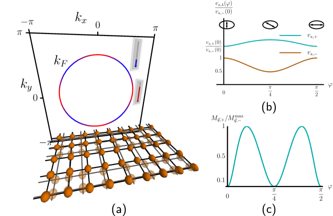
Figure 1: Momentum-dependent effective electronic temperature generated by non-equilibrium acoustic phonons. (a) The lower panel illustrates the instantaneous distortions on a square lattice caused by the excitation of an acoustic phonon mode. The solid (semi-transparent) lines and symbols refer to the undistorted (distorted) lattice. Scattering by non-equilibrium acoustic phonons promotes a momentum-dependent redistribution of electronic quasi-particles, which is translated as a steady-state effective temperature profile that varies along the Fermi surface, depicted in the upper panel (blue and red represent local temperatures that are colder and hotter than the average, respectively). (b) Anisotropic sound velocity $v_{s,\lambda}$ of the two in-plane acoustic phonon modes as a function of the propagation direction $\varphi$. The polarization directions along three high-symmetry directions are also shown. (c) Electron-phonon matrix element $M_{q,-}$ for the low-energy phonon mode as a function of the propagation direction $\varphi$. In this and in the next figures, we set the ratio $(C_{11}-C_{12})/(2C_{66})=1/4$, such that $v_{s,-}(\pi/4)/v_{s,-}(0)=1/2$.

In this paper, we explore an alternative, complementary route to manipulate competing electronic phases on long time scales: the non-equilibrium excitation of acoustic phonons. Although acoustic phonons do not couple directly to light, they can be excited by rapidly applying lattice strain via an interface or via piezoelectric forces Rini et al. (2007); Pezeril et al. (2011); Caviglia et al. (2012); Forst et al. (2015). The small energies required to excite acoustic phonons, as compared to optical phonons, generate less heating. Importantly, while the excited optical phonon modes are usually isotropic, the acoustic phonons studied here are intrinsically anisotropic. As a result, the coupling between the electronic subsystem and the non-equilibrium distribution of acoustic phonons leads to a redistribution of electronic quasiparticles close to the Fermi surface without generating too much heating. As we show below, this redistribution of electronic spectral weight is then translated into an anisotropic effective electronic temperature profile $\delta T_{\mathbf{p}}$ on the Fermi surface, resulting in momentum-selective heating of the low-energy electronic states (see schematic Fig. 1a). The term effective temperature is sharply defined below; for now, we emphasize that it is not the thermodynamic temperature, but a parametrization of the non-equilibrium distribution function that appears on the non-equilibrium gap equations in a similar way as the thermodynamic temperature appears on the equilibrium gap equations.

Our calculations reveal that the precise shape of the effective temperature profile $\delta T_{\mathbf{p}}$ can be tuned by selecting the energy of the excited acoustic phonons. Furthermore, because the anisotropy of $\delta T_{\mathbf{p}}$ is a consequence of the anisotropy of the phonon velocity, the effect discovered here is amplified near a structural phase transition, where the phonon velocity is strongly suppressed along particular directions. This feature makes iron pnictides, cuprates, and heavy fermions promising systems to be manipulated by non-equilibrium acoustic phonons, since some of their phase diagrams display large nematic fluctuations, which cause strong lattice softening Fernandes et al. (2014); Fradkin et al. (2010).

The steady state characterized by a momentum-dependent effective temperature is therefore fundamentally different from any equilibrium state, and allows the control of competing electronic states, particularly in the case of superconductivity competing with a density-wave type of order. The main point is that while generally most low-energy electronic states contribute to the superconducting instability, the competing density-wave instabilities are mostly affected by particular points of the Fermi surface – the “hot spots” connected by the non-zero ordering vector $\mathbf{Q}$. As a result, when the effective local temperature of these hot spots is larger than the average effective temperature across the entire Fermi surface, the competing density-wave instability is suppressed, and superconductivity is enhanced. We demonstrate this very general effect below by explicitly calculating, using the Keldysh formalism, the steady-state phase diagram of a low-energy model widely employed to study competing superconducting and spin-density wave order in the iron pnictides. Finally, we also discuss the conditions that are necessary for the effect discussed here to not be washed away by other relevant relaxation processes, such as those arising from impurity scattering and electron-electron scattering.

II Microscopic model

Our starting point is the electron-phonon Hamiltonian $H=H_{\mathrm{el}}+H_{\mathrm{ph}}+H_{\mathrm{el-ph}}$. Here, $H_{\mathrm{el}}$ describes an interacting electronic system $H_{\text{el}}=H_{0}+H_{\text{int}}$ with kinetic term $H_{0}=\sum_{\mathbf{p}}\xi_{\mathbf{p}}c_{\mathbf{p},\sigma}^{{\dagger}}c_{\mathbf{p},\sigma}$, where the operator $c_{\mathbf{p},\sigma}^{{\dagger}}$ creates an electron with momentum $\mathbf{p}$ and spin $\sigma$ and $\xi_{\mathbf{p}}$ is the band dispersion. The interaction term $H_{\text{int}}$ is responsible for the superconducting and density-wave instabilities of the system, and will be discussed in more details later. The phonons are described by the harmonic term $H_{\mathrm{ph}}=\sum_{\mathbf{q},\lambda}\omega_{\mathbf{q},\lambda}a_{\mathbf{q},\lambda}^{\dagger}a_{\mathbf{q},\lambda}^{\phantom{\dagger}}$, where the operator $a_{\mathbf{q},\lambda}^{{\dagger}}$ creates a phonon with momentum $\mathbf{q}$ and energy $\omega_{\mathbf{q},\lambda}$ in branch $\lambda$. In the long wavelength regime, $\omega_{\mathbf{q},\lambda}=v_{s,\lambda}(\varphi_{\mathbf{q}})|\mathbf{q}|$, where we introduced the sound velocity $v_{s,\lambda}$, which depends on the propagation direction $\varphi_{\mathbf{q}}\equiv\tan^{-1}(q_{y}/q_{x})$. Finally, the electron-phonon term is:

$$H_{\mathrm{el-ph}}=\sum_{\begin{subarray}{c}\mathbf{p},\mathbf{p}^{\prime},\mathbf{q}\\ \mathbf{G},\lambda,\sigma\end{subarray}}\bigl{(}M_{\mathbf{p},\mathbf{p}^{\prime},\mathbf{q},\lambda}\,a_{\mathbf{q},\lambda}^{\dagger}c_{\mathbf{p},\sigma}^{\dagger}c_{\mathbf{p}^{\prime},\sigma}^{\vphantom{\dagger}}\delta_{\mathbf{p}^{\prime}-\mathbf{p}-\mathbf{q}+\mathbf{G}}+\mathrm{h.c.}\bigr{)}$$ (1)

with momentum conserved up to a reciprocal lattice vector $\mathbf{G}$. In the absence of umklapp processes, the matrix element $M_{\mathbf{p},\mathbf{p}^{\prime},\mathbf{q},\lambda}$ is typically approximated, in the long wavelength regime, by Ziman (2001)

$$|M_{\mathbf{p}-\mathbf{p}^{\prime}=\mathbf{q},\lambda}|^{2}\propto\frac{\left(\mathbf{q}\cdot\mathbf{e}_{\mathbf{q},\lambda}\right)^{2}}{v_{s,\lambda}(\varphi_{\mathbf{q}})|\mathbf{q}|}$$ (2)

with transferred momentum $\mathbf{q}$ and phonon polarization $\mathbf{e}_{\mathbf{q},\lambda}$. The polarization and dispersion of the acoustic phonon modes are determined solely by the properties of the elastic tensor. Since many of our systems of interest are tetragonal, the elastic free energy is given by $F=\sum_{\mathbf{q},ij}u_{i}\mathcal{D}_{ij}(\mathbf{q})u_{j}$, where $\mathbf{u}$ is the lattice displacement and $\mathcal{D}_{ij}(\mathbf{q})$ is the symmetric dynamic matrix of a tetragonal system:

$$\mathcal{D}_{ij}(\mathbf{q})=\begin{pmatrix}C_{11}q_{x}^{2}+C_{66}q_{y}^{2}+C_{44}q_{z}^{2}&(C_{12}+C_{66})q_{x}q_{y}&(C_{13}+C_{14})q_{x}q_{z}\\ (C_{12}+C_{66})q_{x}q_{y}&C_{66}q_{x}^{2}+C_{11}q_{y}^{2}+C_{44}q_{z}^{2}&(C_{13}+C_{44})q_{y}q_{z}\\ (C_{13}+C_{44})q_{y}q_{z}&(C_{13}+C_{14})q_{x}q_{z}&C_{44}(q_{x}^{2}+q_{y}^{2})+C_{33}q_{z}^{2}\end{pmatrix}$$ (3)

Here, $C_{ij}$ are the elastic constants. Because our focus is in layered systems, we set $q_{z}=0$ hereafter. Instead of writing the expressions in terms of the three relevant elastic constants $C_{11}$, $C_{12}$, and $C_{66}$, it is convinient to introduce the three coefficients $\mu_{1}=C_{11}+C_{66}$, $\mu_{2}=C_{11}-C_{66}$ and $\mu_{3}=C_{12}+C_{66}$. Diagonalization of the symmetric matrix leads to two phonon branches $\lambda=\pm$; their velocities are given by:

$$v_{s,\pm}(\varphi_{\mathbf{q}})=\frac{1}{\sqrt{2\rho}}\sqrt{\mu_{1}\pm\sqrt{\frac{\mu_{2}^{2}+\mu_{3}^{2}}{2}+\frac{(\mu_{2}^{2}-\mu_{3}^{2})\cos 4\varphi_{\mathbf{q}}}{2}}}$$ (4)

and their polarizations are:

$$\mathbf{e}_{+}\left(\varphi\right) =\frac{1}{\sqrt{2x\left(x+\mu_{2}\cos 2\varphi\right)}}\begin{pmatrix}\mu_{2}\cos 2\varphi+x\\ \mu_{3}\sin 2\varphi\end{pmatrix}$$

$$\mathbf{e}_{-}\left(\varphi\right) =\frac{1}{\sqrt{2x\left(x+\mu_{2}\cos 2\varphi\right)}}\begin{pmatrix}-\mu_{3}\sin 2\varphi\\ \mu_{2}\cos 2\varphi+x\end{pmatrix}$$ (5)

where $\rho$ is the density and $x=\sqrt{\frac{1}{2}(\mu_{2}^{2}+\mu_{3}^{2})+\frac{1}{2}(\mu_{2}^{2}-\mu_{3}^{2})\cos(4\varphi)}$. In the remainder of the paper, we focus our analysis on the low-energy phonon mode, $\omega_{\mathbf{q},-}$, and drop the branch index $\lambda$. The anisotropy of this mode, which is four-fold symmetric, depends on the relative strength of the elastic constants, since $\frac{v_{s}\left(0\right)}{v_{s}\left(\pi/4\right)}=\sqrt{\frac{2C_{66}}{C_{11}-C_{12}}}$. As a result, the phonon anisotropy is stronger in systems close to a tetragonal-to-orthorhombic lattice instability, since in this case either $C_{66}\rightarrow 0$ (corresponding to a $B_{2g}$ deformation of the square lattice) or $C_{11}-C_{12}\rightarrow 0$ (corresponding to a $B_{1g}$ deformation of the square lattice). Because the phase diagrams of the iron pnictides, of some cuprates, and of some heavy fermions display nematic fluctuations Fernandes et al. (2014); Fradkin et al. (2010) related to a $B_{1g}$ tetragonal-to-orthorhombic instability, we focus on the case $\left(C_{11}-C_{12}\right)/2\ll C_{66}$. In this situation, the sound velocity is minimum at $\varphi=\pi/4$ and maximum at $\varphi=0$, as shown in Fig. 1b. The polarization $\mathbf{e}_{\mathbf{q},-}$ of the low-energy phonon mode described by Eq. (4) is transversal at the high-symmetry propagation directions $\varphi=0,\,\frac{\pi}{4},\,\frac{\pi}{2}$, implying that the electron-phonon matrix element $M_{\mathbf{q},-}$ vanishes at these directions. This behavior is shown in Fig. 1c. Note that the anisotropy of $M_{\mathbf{q},-}$, given by Eq. (2), arises both from the anisotropy of the polarization and from the anisotropy of the sound velocity.

III Momentum-dependent effective electronic temperature

III.1 Boltzmann formalism

Having established the properties of the coupling between electrons and phonons, we now discuss how driving the acoustic phonons out of equilibrium affects the low-energy electronic states. Experimentally, a non-equilibrium distribution of acoustic phonons, which we denote by $n_{B}(\omega_{\mathbf{q}})$, can be generated by ultrafast strain of interfaces Rini et al. (2007); Pezeril et al. (2011); Caviglia et al. (2012); Forst et al. (2015); Giannetti et al. (2016). A periodic driving of such non-equilibrium phonons is necessary to establish a steady-state non-thermal phononic distribution, otherwise the phonons would relax back to equilibrium. These out-of-equilibrium phonons inelastically scatter electronic quasi-particles between their momentum eigenstates, resulting in a non-equilibrium electronic distribution function $n_{\xi_{\mathbf{p}}}^{F}$. Theoretically, the latter is given by the solution of the Boltzmann equation $I_{\mathrm{coll}}^{\mathrm{phonon}}[n^{F},n^{B}]=0$, where $I_{\mathrm{coll}}^{\mathrm{phonon}}$ denotes the phonon collision integral:

$$I_{\mathrm{coll}}^{\mathrm{phonon}}[n^{F},n^{B}]=-\sum_{\alpha=\pm}\alpha\int\frac{\mathrm{d}^{2}p^{\prime}}{(2\pi)^{2}}\delta(\xi_{\mathbf{p}}-\xi_{\mathbf{p}^{\prime}}-\alpha\omega_{\mathbf{p}-\mathbf{p}^{\prime}})|M_{\mathbf{p}-\mathbf{p}^{\prime}}|^{2}\left[n_{\xi_{\mathbf{p}}}^{F}n_{-\xi_{\mathbf{p}^{\prime}}}^{F}n_{-\alpha\omega_{\mathbf{p}-\mathbf{p}^{\prime}}}^{B}+n_{-\xi_{\mathbf{p}}}^{F}n_{\xi_{\mathbf{p}^{\prime}}}^{F}n_{\alpha\omega_{{\mathbf{p}-\mathbf{p}^{\prime}}}}^{B}\right]\,,$$ (6)

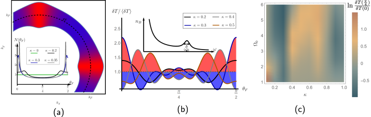
Figure 2: Anisotropic redistribution of electronic state and non-uniform heating of the Fermi surface states. (a) Due to the geometric constraint imposed by momentum conservation, Eq. (7), the electronic states capable of absorbing acoustic phonons are not uniformly distributed around the Fermi surface (black dashed line). States near the red thick (blue thin) regions have a larger (smaller) phase space for phonon scattering. The inset shows the density of electronic states $N\left(\theta_{F}\right)$ available for the scattering of an electron at a Fermi surface angle $\theta_{F}$ by a phonon of energy $\omega_{0}$, for different values of the dimensionless parameter $\kappa\equiv\left(\frac{\omega_{0}}{2\varepsilon_{F}}\right)/\left(\frac{v_{s}(0)}{v_{F}}\right)$. (b) Momentum-dependent temperature profile $\delta T\left(\theta_{F}\right)$, normalized by the average heating $\left\langle\delta T\right\rangle$, for different values of $\kappa$. The phonon non-equilibrium distribution $n_{B}$ is depicted in the inset. We set the ratio $\Omega_{0}\equiv\omega_{0}/2T=5.8$. Due to the scattering of electrons by non-equilibrium phonons, certain regions of the Fermi surface are locally hotter (red shade) or colder (blue shade) than the average. The typical momenta associated with the hot/cold regions change as function of $\kappa$. (c) Color plot of the anisotropy of the non-uniform temperature, as defined by the logarithm of the ratio $\delta T(\pi/4)/\delta T(0)$, as function of the two dimensionless parameters $\kappa$ and $\Omega_{0}$. Blue (yellow) denotes dominant heating near $\theta_{F}=0,\,\pi/2$ ($\theta_{F}=\pi/4$).

Here, we introduced the convention $n_{-x}^{F}=1-n_{x}^{F}$ and $-n_{-x}^{B}=n_{x}^{B}+1$. The physical meaning of the Boltzmann equation is clear: in order for the system to maintain a homogeneous quasi-particle distribution in the steady-state, any deviation of the phonon distribution function from the equilibrium Bose-Einstein function $n_{0,\mathbf{p}}^{B}$ must be compensated by a deviation of the electronic distribution from the Fermi function $n_{0,\mathbf{p}}^{F}$. To focus on the general properties of the mechanism proposed here, we consider small deviations from equilibrium, $n_{\mathbf{p}}^{F/B}=n_{0,p}^{F/B}-(\partial_{\xi_{\mathbf{p}}}n_{0,p}^{F/B})h_{\mathbf{p}}^{F/B}$, and linearize the Boltzmann equation in the functions $h_{\mathbf{p}}^{F/B}$. The resulting integral equation can be conveniently recast as a functional minimization problem, which allows for a direct determination of the electronic non-equilibrium distribution function $h^{F}$ for a given phononic non-equilibrium distribution function $h_{\mathbf{p}}^{B}$ (details in Appendix (A)). Later in Section (V) we discuss the effects of other scattering processes that give additional contributions to the collision integral, such as impurity scattering and electron-electron scattering.

While the equilibrium electronic distribution $n_{0,\mathbf{p}}^{F}$ is determined entirely by the chemical potential $\mu$ and the temperature $T$, the non-equilibrium distribution can be generally parametrized in terms of a momentum-dependent effective temperature $T+\delta T_{\hat{\mathbf{p}}}$, with $\hat{\mathbf{p}}=\mathbf{p}/|\mathbf{p}|$, and an effective chemical potential $\mu+\delta\mu_{\hat{\mathbf{p}}}$, yielding $h_{\mathbf{p}}^{F}=\delta\mu_{\hat{\mathbf{p}}}+\frac{\xi_{\mathbf{p}}}{T}\,\delta T_{\hat{\mathbf{p}}}$. Such a parametrization is particularly useful for the states near the Fermi level, where the energy scales associated with momenta perpendicular and parallel to the Fermi surface are very different. In our problem, because the interaction with a single acoustic phonon cannot modify the chemical potential locally, $\delta\mu_{\hat{\mathbf{p}}}$ is zero. Furthermore, the small energy transfer resulting from the electron-phonon scattering constrains the low-energy electrons to remain near the Fermi surface. As a result, the steady-state non-equilibrium electronic distribution function is completely encoded in the momentum-dependent effective temperature $\delta T_{\hat{\mathbf{p}}}$. Note that this approximation is valid only for a non-current-carrying state; finite currents would require an additional shift of the momentum states. We emphasize that $\delta T_{\hat{\mathbf{p}}}$ is not a thermodynamic temperature, but a convenient parametrization of the distribution function. Its effect on physical observables will be studied in further details in Section (IV).

The precise momentum dependence of the effective electronic temperature $\delta T_{\hat{\mathbf{p}}}$ depends on the type of phonon distribution function $h_{\mathbf{p}}^{B}$. As expected, in the simple case of a uniform heating of the phonons, the solution of the Boltzmann equation gives just a momentum-independent shift of the effective electronic temperature. As we show below, in order to induce anisotropies in $\delta T_{\hat{\mathbf{p}}}$, it is sufficient to excite phonons, isotropically, around a well-defined energy $\omega_{0}$, as the geometrical constraints imposed by momentum and energy conservations, together with the anisotropy of the sound velocity, cause an anisotropic redistribution of quasi-particles.

III.2 Microscopic mechanism for the anisotropic effective temperature

To illustrate this generic effect, we consider a circular Fermi surface of radius $p_{F}$, as shown in Fig. 2a. The Fermi momenta are parametrized by $\mathbf{p}_{F}=p_{F}\left(\cos\theta_{F},\,\sin\theta_{F}\right)$. Momentum conservation enforces a relationship between the initial momentum $\theta_{F}$ and the final momentum $\theta^{\prime}_{F}$, $q=2p_{F}\sin\left(\frac{\theta_{F}-\theta^{\prime}_{F}}{2}\right)$, where $q$ is the phonon momentum. Now, the phonon has a well-defined energy, $q=\omega_{0}/v_{s}\left(\varphi_{\mathbf{q}}\right)$, and a well-defined propagation direction $\varphi_{\mathbf{q}}$, which is also related to the initial and final momenta by $2\varphi_{\mathbf{q}}=\pi+\theta_{F}+\theta^{\prime}_{F}$. As a result, for a given momentum $\theta_{F}$, the allowed values for $\theta^{\prime}_{F}$ are given by the solution of the implicit equation:

$$\kappa=\tilde{v}_{s}\left(\frac{\theta_{F}+\theta^{\prime}_{F}}{2}\right)\sin\left(\frac{\theta_{F}-\theta^{\prime}_{F}}{2}\right)$$ (7)

Here, for convenience, we introduced the dimensionless parameter $\kappa\equiv\left(\frac{\omega_{0}}{2\varepsilon_{F}}\right)/\left(\frac{v_{s}(0)}{v_{F}}\right)$, which relates the typical sound velocity $v_{s}\left(0\right)$, the Fermi velocity $v_{F}$, the excited phonon frequency $\omega_{0}$, and the Fermi energy $\varepsilon_{F}$. The normalized phonon velocity, defined as $\tilde{v}_{s}\left(\varphi\right)\equiv v_{s}\left(\varphi\right)/v_{s}\left(0\right)$, is by definition always smaller than $1$, since the sound velocity is maximum at $\varphi=0$. The key point of Eq. (7) is that the parameter $\kappa$ strongly affects the allowed values for the pair of momenta $\left(\theta_{F},\theta^{\prime}_{F}\right)$. For example, when $\kappa\ll 1$ the solution of Eq. (7) requires the initial and final momenta to be very close, $\theta_{F}^{\prime}\approx\theta_{F}$, whereas when $\kappa>\frac{v_{s}\left(\pi/4\right)}{v_{s}\left(0\right)}$, there is no pair of momenta $\left(\theta_{F},\theta^{\prime}_{F}\right)$ that solves Eq. (7). Note the key role played by the anisotropy in the sound velocity $\tilde{v}_{s}\left(\frac{\theta_{F}+\theta^{\prime}_{F}}{2}\right)$: without it, the equation would only depend on the relative momentum $\theta_{F}-\theta^{\prime}_{F}$.

For intermediate values of $\kappa$, the geometric constraint imposed by Eq. (7) implies that the electronic states that can absorb an acoustic phonon are not equally distributed around the Fermi surface. To quantify this important property, we use Eq. (7) to compute the density of available states, $N\left(\theta_{F}\right)$, for an electron with momentum $\theta_{F}$ scattered by a phonon of energy $\omega_{0}$. The derivation of $N\left(\theta_{F}\right)$ is presented in Appendix (B). In Fig. 2a, we show the behavior of $N\left(\theta_{F}\right)$ projected along the Fermi surface for $\kappa=0.3$: it is clear that Fermi surface states with $\theta_{F}=0,\,\pi/2$ are much more efficient in absorbing the acoustic phonons as compared to the states with $\theta_{F}=\pi/4$. Consequently, the effective temperature along $\theta_{F}=\pi/4$, as caused by phonon scattering, will generally be smaller than along $\theta_{F}=0,\pi/2$. Moreover, the fact that the electron-phonon matrix vanishes for transferred momentum along $\pi/4$ (see Fig. (1)c) causes an additional suppression of the effective temperature along $\theta_{F}=\pi/4$. This is the microscopic origin of the momentum-dependent effective temperature induced by non-equilibrium acoustic phonons. Note from the inset of Fig. 2a that the region of the Fermi surface that is more affected by phonon scattering changes continuously as function of $\kappa$, becoming narrower as $\kappa$ approaches the limiting value $\frac{v_{s}\left(\pi/4\right)}{v_{s}\left(0\right)}\approx 0.5<1$. Consequently, the degree of anisotropy in the effective temperature is controlled by the energy of the excited phonons $\omega_{0}$. Since $\kappa\sim\mathcal{O}(1)$, the relevant phonon energies are always much smaller than the Fermi energy, $\omega_{0}/\varepsilon_{F}\sim\mathcal{O}(v_{s}(0)/v_{F})$.

III.3 Boltzmann result for the anisotropic effective temperature

The general analysis above is confirmed by explicit solution of the Boltzmann equation for $\delta T_{\mathbf{p}}$. In the case of phonons excited near an energy $\omega_{0}$, the non-equilibrium bosonic distribution function is modeled as (see the inset in Fig. 2b):

$$h_{\mathbf{q}}^{B}=W_{B}\,\frac{\delta}{\delta^{2}+\bigl{(}\frac{\omega_{\mathbf{q}}}{2T}-\Omega_{0}\bigr{)}^{2}}\,.$$ (8)

Here, the parameter $\delta\ll 1$ represents the energy width of the excited phonons, $W_{B}$ is an overall amplitude corresponding to the number of bosons excited by the external drive, and $\Omega_{0}\equiv\frac{\omega_{0}}{2T}$ . In Fig. 2b, we show the momentum dependence of the effective temperature profiles $\delta T(\theta_{F})$ obtained by solving the Boltzmann equation for a fixed $\Omega_{0}$ as function of the parameter $\kappa$. For small values of $\kappa$, the anisotropy (as measured by the ratio $\delta T(\frac{\pi}{4})/\delta T(0)$) is mild, with the states with momentum $\theta_{F}=\pi/4$ only slightly colder than those with momenta $\theta_{F}=0,\,\pi/2$. Upon increasing $\kappa$, the anisotropy is clearly increased – in particular, the maximum anisotropy, for $\kappa\approx 0.3$, takes place when the $\theta_{F}=0,\,\pi/2$ states are the hottest states at the Fermi surface. Upon further increasing $\kappa$, the hottest region of the Fermi surface moves back towards the diagonal, but the amplitude of the anisotropy decreases. Remarkably, the changes in $\delta T(\theta_{F})$ as function of $\kappa$ are nearly insensitive to the value of $\Omega_{0}$, as shown in Fig. 2c.

This behavior of $\delta T(\theta_{F})$ is in qualitative agreement with the geometrical analysis of Fig. 2a, which shows that the largest density of electronic states capable of absorbing a phonon moves towards the Fermi surface region near $\theta_{F}=0,\,\pi/2$ and then back towards $\theta_{F}=\pi/4$ as $\kappa$ increases. The fact that the amplitude of the anisotropy is not monotonic can be attributed to the fact that the maximum of the density $N(\theta_{F})$ becomes not only larger but also narrower as $\kappa$ increases, while the distribution function (8) is sensitive to a window of energies centered around $\omega_{0}$. Furthermore, the small changes near $\theta_{F}=\pi/4$ as function of $\kappa$ are a consequence of the numerator of the electron-phonon matrix element in Eq. (2) vanishing for transferred momentum $\pi/4$.

IV Impact on competing electronic phases

We have seen that electrons that interact with out-of-equilibrium acoustic phonons develop an anisotropic non-equilibrium distribution that can be characterized by a momentum dependent effective electronic temperature. We now show that this can be used as a tool to control and manipulate competing electronic states in correlated systems. The idea is that, by tuning the excited phonon energy $\omega_{0}$ (proportional to the parameter $\kappa$ discussed above), one can in principle selectively heat certain regions of the Fermi surface. While applicable to any form of non-isotropic order, this is particularly relevant for density-wave instabilities, which are generally governed by the electronic states near the hot spots $\mathbf{k}_{\mathrm{hs}}$ – points of the Fermi surface separated by the density-wave ordering vector $\mathbf{Q}$, $\xi_{\mathbf{k}_{\text{hs}}}=-\xi_{\mathbf{k}_{\text{hs}}+\mathbf{Q}}$. In this case, an appropriate momentum-dependent effective temperature profile can be applied to selectively melt the density-wave state while preserving other homogeneous ordered phases.

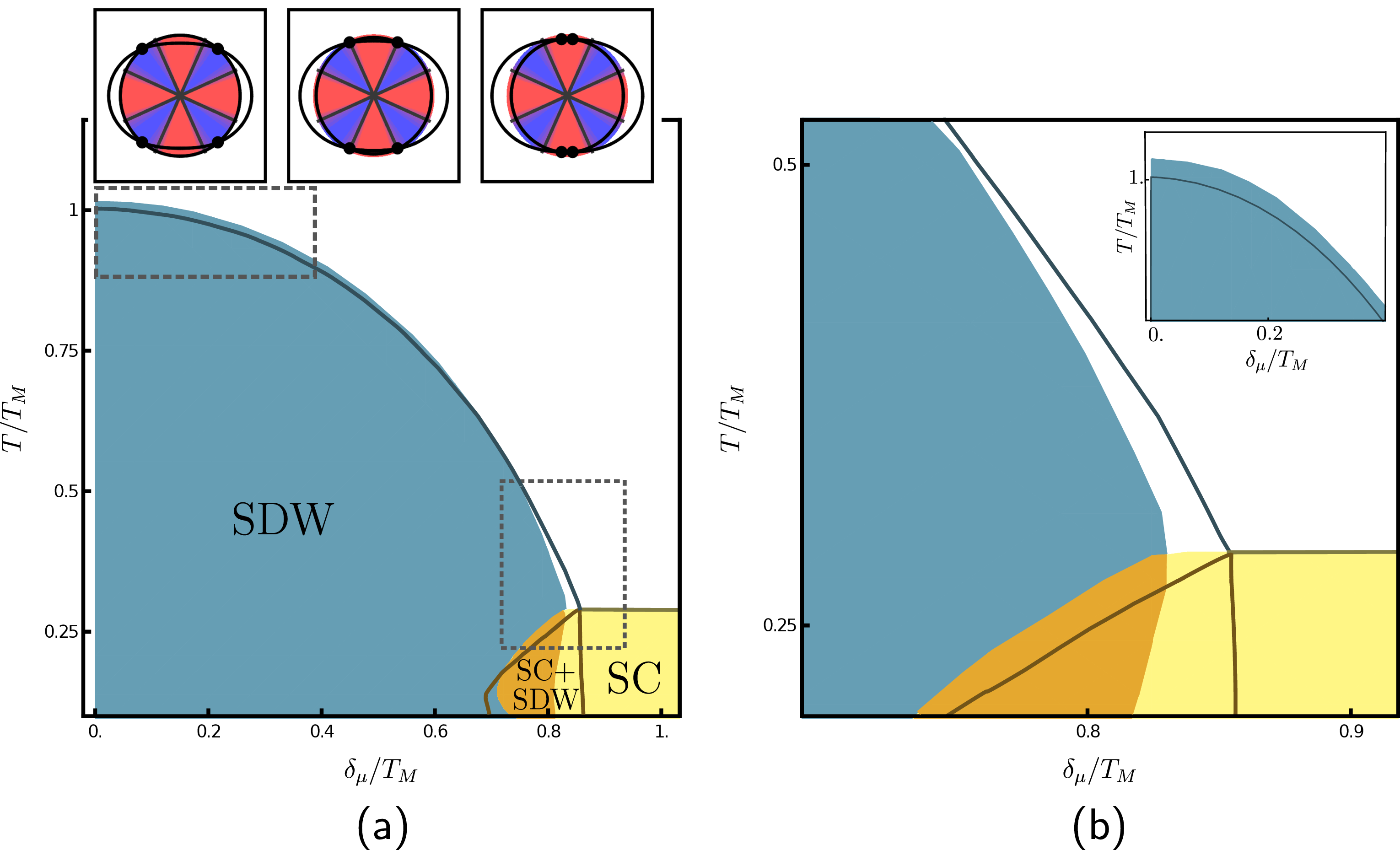
Figure 3: Non-equilibrium steady-state phase diagram for competing superconductivity (SC) and spin-density wave (SDW). The steady-state non-equilibrium phase diagram for the two-band model of the iron pnictides is shown in panel (a), and the highlighted regions are zoomed in panel (b). It contains phases with SDW (cyan), SC (yellow) and coexistent SDW+SC (orange) order. The inset shows the superimposed circular hole-like and elliptical electron-like Fermi pockets, with the latter displaced by the SDW ordering vector $\mathbf{Q}$. The crossing points are the hot spots $\mathbf{k}_{\text{hs}}$, which govern the SDW instability; their positions are controlled by the parameter $\delta_{\mu}$, which also determines the carrier concentration. The non-equilibrium phase diagram was obtained for the anisotropic effective temperature profile $\delta T\left(\theta_{F}\right)$ shown in Fig. 2b (here we set $\kappa=0.27$) and illustrated in the inset (red and blue denote regions hotter and colder than the average heating $\left\langle\delta T\right\rangle$, respectively). For comparison, we also show the equilibrium phase diagram (solid lines) shifted by the average heating $\left\langle\delta T\right\rangle/T_{M}\approx 0.1$. Here, we set $\delta_{m}/T_{M}=0.9$. All quantities are expressed in terms of the equilibrium SDW transition temperature $T_{M}$ for $\delta_{\mu}=0$.

Although generic, this concept of selective melting can be nicely demonstrated by an explicit calculation for the case of competing spin-density wave (SDW) and $s^{+-}$ superconductivity (SC) in the iron pnictides. We emphasize that our goal here is not to provide a microscopically calculated phase diagram for a specific iron pnictide material, but rather to use a transparent low-energy model to demonstrate the general concept proposed here. In this spirit, an effective low-energy model widely employed to study the SDW-SC competition in the pnictides is a two-band model with one circular hole pocket at the center of the Fe square-lattice Brillouin zone, and one elliptical electron pocket centered at the SDW ordering vector $\mathbf{Q}$ Fernandes and Chubukov (2017). The non-interacting Hamiltonian $H_{0}$ then contains two bands that can be conveniently parametrized as $\xi_{h,\mathbf{k}}=\varepsilon_{0}-\frac{k^{2}}{2m}$ and $\xi_{e,\mathbf{k}+\mathbf{Q}}=-\xi_{h,\mathbf{k}}-\delta_{\mu}-\delta_{m}\cos 2\theta$. The parameters $\delta_{\mu}$ (proportional to the electronic occupation number) and $\delta_{m}$ (proportional to the ellipticity of the electron pocket) serve as a measure of the nesting condition between the two bands.

The two leading instabilities arising from $H_{\mathrm{el}}$ are the $s^{+-}$ SC instability, characterized by two uniform gaps of opposite signs in the two bands, and the SDW instability Fernandes and Chubukov (2017). The corresponding interactions projected onto these two channels are denoted by $V_{\mathrm{SC}}$ and $V_{\mathrm{SDW}}$, respectively. While the former is sensitive to all Fermi surface states, the latter is governed by the hot spots. When $|\delta_{\mu}|<|\delta_{m}|$, there are four pairs of hot spots located at the Fermi surface angles multiples of $\theta_{\mathrm{hs}}=\frac{1}{2}\arccos(-\delta_{\mu}/\delta_{m})$, whereas when $\left|\delta_{\mu}\right|>\left|\delta_{m}\right|$, there are no hot spots. Thus, for a fixed $\delta_{m}$, increasing $\left|\delta_{\mu}\right|$ makes nesting poorer, which suppresses the SDW instability. The $\left(\delta_{\mu},T\right)$ equilibrium phase diagram of this model is shown by the solid lines in Fig. 3 for fixed $\delta_{m}$. In this plot, the transition lines have been shifted to mimic a non-zero average uniform heating, as explained below.

To obtain the phase diagram of the non-equilibrium steady state in which the electrons interact with a distribution of non-equilibrium acoustic phonons, we use the Keldysh formalism. The main result, derived in Appendix (C), can be explained in terms of the self-consistent gap equations governing the SC and SDW instabilities. Let us denote the corresponding order parameters by $\Delta$ and $M$. In the Keldysh language, they correspond to classical source fields. The linearized self-consistent equations for $M$ and $\Delta$, derived using the Keldysh approach, are given by:

$$M =2V_{\mathrm{SDW}}\int\frac{\mathrm{d}^{2}p}{\left(2\pi\right)^{2}}\left[\frac{f\left(\xi_{h,\mathbf{p}}\right)-f\left(\xi_{e,\mathbf{p+Q}}\right)}{\xi_{h,\mathbf{p}}-\xi_{e,\mathbf{p+Q}}}\right]M$$

$$\Delta =V_{\mathrm{SC}}\int\frac{\mathrm{d}^{2}p}{\left(2\pi\right)^{2}}\left[\frac{f\left(\xi_{h,\mathbf{p}}\right)}{\xi_{h,\mathbf{p}}}+\frac{f\left(\xi_{e,\mathbf{p+Q}}\right)}{\xi_{e,\mathbf{p+Q}}}\right]\Delta$$ (9)

The key point is that the function $f\left(\xi_{\mathbf{p}}\right)$, which relates the advanced, retarded, and Keldysh components of the electronic Green’s function, $G^{K}=f\left(G^{R}-G^{A}\right)$, is given in terms of the non-equilibrium electronic distribution function $n_{\xi_{\mathbf{p}}}^{F}$ by $f\left(\xi_{\mathbf{p}}\right)=1-2n_{\xi_{\mathbf{p}}}^{F}$. If the system was in equilibrium, the function $f$ would acquire the familiar form $f\left(\xi\right)=\tanh\left(\frac{\beta\xi}{2}\right)$, and Eqs. (9) would reduce to the standard equilibrium gap equations. Out of equilibrium, however, $f\left(\xi_{\mathbf{p}}\right)$ contains information about the non-thermal distribution of electrons, which in turn is parametrized in terms of the effective momentum-dependent temperature $T+\delta T_{\hat{\mathbf{p}}}$. Thus, mathematically, the Keldysh formalism reveals that the effect of the coupling between electrons and non-equilibrium acoustic phonons in this problem can be cast as self-consistent gap equations that have the same form as the equilibrium gap equations, but with the thermodynamic temperature $T$ replaced by the effective temperature $T+\delta T_{\hat{\mathbf{p}}}$, where $T$ is the temperature of a bath to which both the acoustic phonons and the electrons are coupled (such a bath could be due to optical phonons or other degrees of freedom in the system). This justifies associating $\delta T_{\hat{\mathbf{p}}}$ to an effective electronic temperature. Note that this microscopic approach recovers the phenomenological one introduced by Eliashberg and others in Refs. Eliashberg (1960); Eliashberg and Ivlev (1986), which correctly predicted the enhancement of $T_{c}$ in SC thin films irradiated by microwaves.

We can now use these gap equations to calculate the SC-SDW phase diagram for electrons subject to a momentum dependent effective temperature $\delta T\left(\theta_{F}\right)$. This should be understood, in the same spirit as Refs. Eliashberg (1960); Eliashberg and Ivlev (1986), as a steady-state non-equilibrium phase diagram, since without driving, at long enough times, the system will relax back to equilibrium. In this regard, the transition temperatures correspond to the temperatures of the bath discussed in the paragraph above. Because the linearized gap equations (9) can only give the leading instability of the system, to study the competition between SC and SDW we must also included higher order terms of the non-linear gap equations, as explained in Appendix (C).

In what follows, we use the profile $\delta T\left(\theta_{F}\right)/\left\langle\delta T\right\rangle$ calculated in the previous section for $\kappa=0.27$ and $\Omega_{0}=5.8$ , corresponding to dominant heating around $\theta_{F}=0,\,\pi/2$ (see Fig. 2b). The steady-state phase diagram is shown by the shaded regions in Fig. 3. To make the comparison with the equilibrium phase diagram more meaningful, and to highlight the impact of non-uniform heating, the equilibrium temperature was shifted by the average heating $\left\langle\delta T\right\rangle\equiv\int\frac{d\theta_{F}}{2\pi}\,\delta T\left(\theta_{F}\right)$, which depends on the external drive.

On the overdoped side of the phase diagram ($\delta_{\mu}/T_{M}\gtrsim 0.75$), where only SC is present, we find that the SC $T_{c}$ is unaffected by the non-uniform heating. This is because the $s^{+-}$ SC instability has equal contributions from all electronic states at the Fermi surface, since the gap function is uniform. As a result, $T_{c}$ is sensitive only to the average temperature around the Fermi surface, $\left\langle\delta T\right\rangle$. In contrast, on the very underdoped side of the phase diagram (near $\delta_{\mu}=0$), where only SDW is present, we observe that the SDW transition temperature $T_{M}$ increases for non-uniform heating, because the SDW instability is dominated by the hot spots of the Fermi surface. For these doping levels, as shown in the inset of Fig. 3a, the hot spots are located near $\theta_{F}=\pi/4$, where the local effective temperature $\delta T(\frac{\pi}{4})$ oscillates weakly around the average $\left\langle\delta T\right\rangle$. Electrons near the hot spots experience less heating than the average.

As $\delta_{\mu}$ (i.e. doping) increases, the hot spots move towards the $\theta_{F}=\pi/2$ direction; this behavior is also seen experimentally in certain pnictides Liu et al. (2010). Because the local temperature in this Fermi surface region is larger than the average one, $T_{M}$ decreases. More interestingly, as highlighted in Fig. 3b, superconductivity is favored and $T_{c}$ systematically increases near the optimal doping regime $\delta_{\mu}/T_{M}\approx 0.75$, as compared to its equilibrium value. Because the SC order is unaffected by the non-uniform heating, this enhancement of $T_{c}$ is a direct consequence of the suppression of the SDW transition $T_{M}$. This clearly illustrates that a momentum-dependent effective electronic temperature is able to shift the balance between competing orders.

V Discussion and conclusions

In this paper we explored a novel framework to manipulate and control correlated electronic systems out of equilibrium. In particular, we demonstrated that non-equilibrium acoustic phonons excited around a well-defined energy lead to a non-uniform redistribution of electronic states around the Fermi surface. This manifests as a momentum-dependent effective temperature characterizing the non-equilibrium distribution function. Our theoretical result is robust, as it stems from geometric constraints imposed by energy and momentum conservation, together with the intrinsic anisotropy of the sound velocity. It reveals a hitherto unexplored path to manipulate correlated states via pump-and-probe experiments, which have so far been mostly focusing on the coherent excitation of optical phonons. In contrast to the latter, heating effects are expected to be much weaker in the case of acoustic phonons, since the energies involved are significantly smaller.

The application of this interesting idea to realistic systems requires several conditions to be satisfied. First, it is necessary to create a non-thermal distribution of acoustic phonons. Recent experimental advances in the ultrafast strain manipulation of interfaces and heterostructures, including the production of shock waves, provide a promising route forward Rini et al. (2007); Pezeril et al. (2011); Caviglia et al. (2012); Forst et al. (2015); Giannetti et al. (2016). While in this paper we focused on the excitation of phonons with a well-defined energy, similar results will hold for phonons with a well-defined momentum propagation. Second, this non-thermal phonon population has to be periodically driven, since the phonons themselves thermalize, usually in the time scale of several hundrets of picoseconds Klett and Rethfeld (2017). Third, it is necessary to ensure that other scattering processes do not relax the electronic momenta too fast, washing away the anisotropic effective temperature induced by the coupling to the non-equilibrium acoustic phonons.

This is a crucial condition that deserves further consideration. The usual scattering processes considered other than scattering by phonons (or by other collective bosonic modes) are impurity scattering and electron-electron scattering. Their effect on the electronic distribution function can be obtained by including the corresponding collision integrals in the Boltzmann equation. While a detailed solution of the full Boltzmann equation is beyond the scope of this work, there are important qualitative points that can be made (details in Appendix (D)). In the case of impurity scattering, as long as the energy of the excited phonons is comparable to the thermodynamic temperature ($\Omega_{0}=\omega_{0}/(2T)\gtrsim 1$ in Fig. 2c), the anisotropy of the effective electronic temperature generated by the coupling to the acoustic phonons should persist even when the electron-impurity matrix element is of the same order as the electron-phonon matrix element. Importantly, both matrix elements can in principle be controlled: while the former is proportional to the concentration of impurities (which is suppressed by annealing), the latter is inversely proportional to the sound velocity (which is enhanced near a structural phase transition).

As for the case of electron-electron scattering, it is essential to distinguish two different processes, namely, energy relaxation and momentum relaxation. The former causes the electronic subsystem to thermalize, and is usually assumed to be very fast (in the femtosecond time scale) in phenomenological models widely employed to describe the relaxation of materials taken out of equilibrium, such as the two-temperature model. Nevertheless, such an assumption of a very fast electron thermalization may not hold for several systems. Theoretically, previous works studying the solution of the Boltzmann equation with both electron-phonon and electron-electron scattering Groeneveld et al. (1995); Kabanov and Alexandrov (2008) revealed that, for a wide range of parameters, electron-electron scattering is actually unable to bring the electrons to a thermal distribution in the time scales of the electron-phonon relaxation time. Experimental signatures of this effect were observed early on for several simple metals Groeneveld et al. (1995). More recently, it has been argued that a similar effect may take place in cuprates Giannetti et al. (2016). Importantly, these works show that the electron-electron energy relaxation time can become comparable or even longer than the electron-phonon relaxation time, depending on materials properties and experimental conditions. For the framework that we propose here, because the relevant electronic states remain near the Fermi energy due to the small energy transferred by the acoustic phonons, the electron-electron energy relaxation is expected to be longer due to Pauli’s principle. Regardless of its time scale, it is important to note that this energy relaxation process does not wash away the anisotropy of the effective electronic temperature, as it does not promote momentum relaxation. In fact, it actually helps establishing an effective electronic temperature, as it brings the electrons to a nearly thermal distribution, which justifies the expansion of the non-equilibrium electronic distribution function around a thermal distribution (as we assumed in Sec. IIIA). The process that is harmful to the anisotropy of the effective temperature is the electron-electron momentum relaxation, which generally takes place on longer time scales than the energy relaxation. In two-dimensional systems, the difference between the two relaxation times is expected to be even larger, due to the dominance of scattering processes involving zero momentum transfer Chubukov and Maslov (2004).

Among several possible applications of the anisotropic effective electronic temperature generated by non-equilibrium acoustic phonons, we showed here that it can be employed to selectively melt competing electronic states, particularly in the case of unconventional superconductivity competing with a density-wave type of order. The potential enhancement of $T_{c}$ by non-equilibrium acoustic phonons complements previous approaches in which SC is enhanced by optical phonons or microwave radiation. These results also open a broad set of questions that deserve further investigation. An interesting issue is the impact of non-equilibrium acoustic phonons on electronic orders that directly couple to the lattice, such as nematic orders and charge-density waves. Furthermore, nodal superconducting states are ideal candidates to be manipulated by a momentum-dependent effective temperature, since the nodal quasi-particles, which determine the low-energy excitation spectrum, can experience a different local effective temperature than the average. Finally, while here we focused on long-range order, a non-uniform effective electronic temperature should also impact the low-energy charge and magnetic fluctuation spectra, which influence the pairing state.

Appendix A Solution of the Boltzmann equation

As discussed in the main text, the Boltzmann equation is given by:

$$I_{\mathrm{coll}}^{\mathrm{phonon}}[n^{F},n^{B}]=-\sum_{\alpha=\pm}\alpha\int\frac{\mathrm{d}^{2}p^{\prime}}{(2\pi)^{2}}\delta(\xi_{\mathbf{p}}-\xi_{\mathbf{p}^{\prime}}-\alpha\omega_{\mathbf{p}-\mathbf{p}^{\prime}})|M_{\mathbf{p}-\mathbf{p}^{\prime}}|^{2}\left[n_{\xi_{\mathbf{p}}}^{F}n_{-\xi_{\mathbf{p}^{\prime}}}^{F}n_{-\alpha\omega_{\mathbf{p}-\mathbf{p}^{\prime}}}^{B}+n_{-\xi_{\mathbf{p}}}^{F}n_{\xi_{\mathbf{p}^{\prime}}}^{F}n_{\alpha\omega_{{\mathbf{p}-\mathbf{p}^{\prime}}}}^{B}\right]=0$$ (10)

Linearization of the kernel leads to

$$\left[n_{\xi_{\mathbf{p}}}^{F}n_{-\xi_{\mathbf{p}^{\prime}}}^{F}n_{-\alpha\omega_{\mathbf{p}-\mathbf{p}^{\prime}}}^{B}+n_{-\xi_{\mathbf{p}}}^{F}n_{\xi_{\mathbf{p}^{\prime}}}^{F}n_{\alpha\omega_{\mathbf{p}-\mathbf{p}^{\prime}}}^{B}\right]\approx-\frac{1}{8}\frac{h_{\xi_{\mathbf{p}}}^{F}-h_{\xi_{\mathbf{p}^{\prime}}}^{F}-\alpha h_{\omega_{\mathbf{p}-\mathbf{p}^{\prime}}}^{B}}{\cosh\left[\frac{\beta\xi_{\mathbf{p}}}{2}\right]\cosh\left[\frac{\beta\xi_{\mathbf{p}^{\prime}}}{2}\right]\sinh\left[\frac{\beta\alpha\omega_{\mathbf{p}-\mathbf{p}^{\prime}}}{2}\right]}$$ (11)

where we used the fact that $h_{\alpha\omega_{q}}^{B}=\alpha h_{\omega_{q}}^{B}$. Our goal is to find the fermionic distribution $h^{F}$ that solves the Boltzmann equation for a given phononic distribution $h^{B}$. It is convenient to work with a functional $\mathcal{F}\left[h^{F}\right]$ whose minimization with respect to $h^{F}$ gives the Boltzmann equation. We find:

$$\mathcal{F}\left[h^{F}\right]=\int\frac{\mathrm{d}^{2}p}{(2\pi)^{2}}\int\frac{\mathrm{d}^{2}p^{\prime}}{(2\pi)^{2}}\sum_{\alpha=\pm}\alpha\delta(\xi_{\mathbf{p}}-\xi_{\mathbf{p}^{\prime}}-\alpha\omega_{\mathbf{p}-\mathbf{p}^{\prime}})\frac{|M_{\mathbf{p}-\mathbf{p}^{\prime}}|^{2}}{16}\frac{\left(h_{\xi_{\mathbf{p}}}^{F}-h_{\xi_{\mathbf{p}^{\prime}}}^{F}\right)^{2}-2\alpha h_{{\mathbf{p}-\mathbf{p}^{\prime}}}^{B}h_{\xi_{\mathbf{p}}}^{F}+2\alpha h_{{\mathbf{p}^{\prime}-\mathbf{p}}}^{B}h_{\xi_{\mathbf{p}^{\prime}}}^{F}}{\cosh\left[\frac{\xi_{\mathbf{p}}}{2T}\right]\cosh\left[\frac{\xi_{\mathbf{p}^{\prime}}}{2T}\right]\sinh\left[\frac{\xi_{\mathbf{p}}-\xi_{\mathbf{p}^{\prime}}}{2T}\right]}$$ (12)

To proceed, we note that, since the energy of the excited acoustic phonons is much smaller than the Fermi energy, we can linearize the electronic dispersion in the vicinity of the Fermi surface. Then, it is convenient to split the momentum into components perpendicular and parallel to the Fermi surface (FS), yielding $\int\mathrm{d}^{2}p/(2\pi)^{2}=\int\mathrm{d}\theta/(2\pi)N_{F}(\theta)\int\mathrm{d}\xi_{p}$. As a result, the electronic states close to the Fermi level, the phonon dispersion, and the electron-phonon-matrix element Eq. (2) depend only on the transferred momenta longitudinal to the Fermi surface $\theta$ and $\theta^{\prime}$. For simplicity, hereafter we will keep the notation $\omega_{q}=\omega_{\mathbf{p}_{F}(\theta)-\mathbf{p}_{F}(\theta^{\prime})}$. Finally, introducing the parametetrization $h_{\mathbf{p}}^{F}=\delta\mu_{\hat{\mathbf{p}}}+\frac{\xi_{\mathbf{p}}}{T}\,\delta T_{\hat{\mathbf{p}}}$, we can evaluate the energy integration in the functional Eq. (12), obtaining a functional that depends only on the longitudinal momenta:

$$\mathcal{F}\left[h^{F}\right]=\iint\frac{\mathrm{d}\theta\mathrm{d}\theta^{\prime}}{(2\pi)^{2}}N_{F}(\theta)N_{F}(\theta^{\prime})\frac{\beta\omega_{q}|M_{\mathbf{q}}|^{2}}{4\sinh^{2}(\frac{\beta\omega_{q}}{2})}\left\{\left(\frac{\beta\omega_{q}}{2}\right)^{2}\left[\left(\delta T_{\hat{\mathbf{p}}}+\delta T_{\hat{\mathbf{p}}^{\prime}}\right)\right]^{2}\right.\\ \left.+\frac{1}{3}\left[\pi^{2}+\left(\frac{\beta\omega_{q}}{2}\right)^{2}\right]\left(\delta T_{\hat{\mathbf{p}}}-\delta T_{\hat{\mathbf{p}}^{\prime}}\right)^{2}-\beta\omega_{q}h_{\mathbf{q}}^{B}\left[\delta T_{\hat{\mathbf{p}}}+\delta T_{\hat{\mathbf{p}}^{\prime}}\right]\right\}$$ (13)

Because the effective chemical potential $\delta\mu_{\hat{\mathbf{p}}}$ does not appear in the functional, it follows that a non-equilibrium distribution of acoustic phonons cannot change the chemical potential. Note that while small momentum scattering is suppressed by the electron-phonon matrix element Eq (2), this effect is compensated by the amount of available thermal states to scatter, which is proportional to $1/\sinh^{2}(\beta\omega_{q}/2)$.

To minimize the functional, it is convenient to use the Fourier representation of $\delta T\left(\theta\right)$:

$$\delta T(\theta)-\delta T(\theta^{\prime}) =-2\sum_{n}\delta T_{n}\sin\left(n\frac{\theta-\theta^{\prime}}{2}\right)\sin\left(n\frac{\theta+\theta^{\prime}}{2}\right)$$ (14a)

$$\delta T(\theta)+\delta T(\theta^{\prime}) =2\sum_{n}\delta T_{n}\cos\left(n\frac{\theta-\theta^{\prime}}{2}\right)\cos\left(n\frac{\theta+\theta^{\prime}}{2}\right)$$ (14b)

The Fourier components $\delta T_{n}$ can then be found by solving the matrix equation $\sum_{m}K_{nm}\delta T_{m}=D_{n}$, with:

$$D_{n}=-\iint\frac{\mathrm{d}\theta\mathrm{d}\theta^{\prime}}{(2\pi)^{2}}N_{F}(\theta)N_{F}(\theta^{\prime})\frac{\beta\omega_{q}|M_{\mathbf{q}}|^{2}}{4\sinh^{2}(\frac{\beta\omega_{q}}{2})}2\beta\omega_{q}h^{B}(\omega_{q})\cos\left(n\frac{\theta-\theta^{\prime}}{2}\right)\cos\left(n\frac{\theta+\theta^{\prime}}{2}\right)$$ (15)

and

$$K_{nm}=\iint\frac{\mathrm{d}\theta\mathrm{d}\theta^{\prime}}{(2\pi)^{2}}N_{F}(\theta)N_{F}(\theta^{\prime})\frac{\beta\omega_{q}|M_{\mathbf{q}}|^{2}}{4\sinh^{2}(\frac{\beta\omega_{q}}{2})}\\ \left\{\left(\frac{\beta\omega_{q}}{2}\right)^{2}4\cos\left(n\frac{\theta-\theta^{\prime}}{2}\right)\cos\left(n\frac{\theta+\theta^{\prime}}{2}\right)\cos\left(m\frac{\theta-\theta^{\prime}}{2}\right)\cos\left(m\frac{\theta+\theta^{\prime}}{2}\right)\right.\\ \left.+\frac{1}{3}\left[\pi^{2}+\left(\frac{\beta\omega_{q}}{2}\right)^{2}\right]4\sin\left(n\frac{\theta-\theta^{\prime}}{2}\right)\sin\left(n\frac{\theta+\theta^{\prime}}{2}\right)\sin\left(m\frac{\theta-\theta^{\prime}}{2}\right)\sin\left(m\frac{\theta+\theta^{\prime}}{2}\right)\right\}$$ (16)

In the main text, we numerically solved these equations using the following expressions for the phononic distribution function and matrix element:

$$h^{B}(\omega_{q}) =W_{B}\,\frac{\delta}{\delta^{2}+\left[\frac{\omega_{q}}{2T}-\Omega_{0}\right]^{2}}\,$$ (17)

$$\omega_{q}|M_{\mathbf{q}}|^{2} =m_{0}(\theta,\theta^{\prime})q^{2}=\tilde{m}_{0}(\theta,\theta^{\prime})\sin\left(\frac{\theta-\theta^{\prime}}{2}\right)$$ (18)

Note that the behavior of the overall function $m_{0}(\theta,\theta^{\prime})$ is given by Fig. 1 with $2\varphi=\theta+\theta^{\prime}$ and that for $\varphi\neq 0,\pi/4,\pi/2$ drops from the equations, since it appears as a weight in both $K_{nm}$ and $D_{n}$. The phonon energy is given in terms of the dimensionless parameters and the function $\tilde{v}_{s}$ defined in the main text:

$$\frac{1}{2}\beta\omega_{q}=\frac{\Omega_{0}}{\kappa}\,\tilde{v}_{s}\left(\frac{\theta+\theta^{\prime}}{2}\right)\sin\left(\frac{\theta-\theta^{\prime}}{2}\right)$$ (19)

Consequently, the functional depends only on three parameters, $\Omega_{0}$, $\delta$, and $\kappa$. Prefactors appearing in $h^{B}$, in the matrix element $|M_{\mathbf{q}}|^{2}$, and in the density of states can be conveniently absorbed into the average heating $\left\langle\delta T\right\rangle$.

Appendix B Analysis of the geometric constraint

In the main text, we derived the geometric constraint on the initial and final electronic momenta $\theta_{F}$, $\theta_{F}^{\prime}$ due to the energy-momentum conservation associated with electron-phonon scattering:

$$\kappa=\tilde{v}_{s}\left(\frac{\theta_{F}+\theta^{\prime}_{F}}{2}\right)\sin\left(\frac{\theta_{F}-\theta^{\prime}_{F}}{2}\right)$$ (20)

An important quantity is the density of available scattering states $\theta^{\prime}_{F}$ for a given momentum $\theta_{F}$, which we denoted by $N(\theta_{F})$. For a given angle $\theta_{0}$ in the first quadrant, there are at least two angles $\theta_{1}$ and $\theta_{2}$ also in the first quadrant that satisfy Eq. (20), with $\theta_{1}>\theta_{0}>\theta_{2}$. In order to determine $N(\theta_{F})$, let us introduce two “rotated” variables $\delta\theta=(\theta_{1}-\theta_{2})/2$ and $\varphi=(\theta_{1}+\theta_{2})/2$, such that condition (20) becomes $\kappa=\tilde{v}_{s}(\varphi)\sin(\delta\theta)$. Note that $\varphi$ is, up to a translation by $\pi/2$, the angle corresponding to the phonon propagation direction. In terms of these variables, it is straightforward to obtain the solution to Eq. (20), $\delta\theta(\varphi)=\mathrm{arcsin}(\kappa/\tilde{v}_{s}(\varphi))$. Thus, for a given phonon direction $\varphi$, the two electronic scattering angles are given by $\theta_{1/2}=\Phi_{\pm}(\varphi)$, with $\Phi_{\pm}(\varphi)=\varphi\pm\delta\theta(\varphi)$.

It is now straightforward to count the number of all possible electronic scattering pairs by integrating over all available phonon directions:

$$N(\theta)=\frac{1}{2}\sum_{\alpha=\pm 1}\int\mathrm{d}\varphi\,\delta\left[\theta-\Phi_{\alpha}(\varphi)\right].$$ (21)

yielding:

$$N(\theta)=\frac{1}{2}\sum_{\alpha=\pm 1}\frac{1}{1+\alpha\left(\frac{\partial\delta\theta}{\partial\varphi}\right)_{\varphi=\Phi_{\alpha}^{-1}(\theta)}}$$ (22)

Alternatively, we can also express the density of scattering states as function of the phonon direction $\varphi$. In this case,

$$N\left(\varphi\right) =\frac{1}{2}\left[\left(\frac{\partial\phi(\varphi)}{\partial\varphi_{q}}\right)^{-1}+\left(\frac{\partial\phi^{\prime}(\varphi)}{\partial\varphi_{q}}\right)^{-1}\right]$$

$$=\frac{1}{1-\frac{\kappa^{2}}{\tilde{v}_{s}^{2}-\kappa^{2}}\left(\frac{\tilde{v}_{s}^{\prime}}{\tilde{v}_{s}}\right)^{2}}.$$ (23)

In Fig. 2 of the main text, we plotted $N\left(\theta\right)$ for different values of $\kappa$. Note that for $\kappa>\mathop{\mathrm{Min}}\limits_{\varphi\in[0,\pi/2]}\sqrt{\frac{v_{s}^{4}}{v_{s}^{2}+(v_{s}^{\prime})^{2}}}$ the expressions above do not apply and the density needs to be redefined, since for a given angle $\varphi$, four different pairs $(\theta_{F},\theta_{F}^{\prime})$ exist. In our case this happens for about $\kappa\approx 0.365$.

In Fig. 4, we plot the density of available scattering solutions as function of the phonon direction $\varphi$, $N\left(\varphi\right)$. Clearly, for all values of $\kappa$, the main contribution comes from phonons with $\varphi\approx\varphi_{0}$, where $\varphi_{0}$ is the angle for which $\sqrt{\frac{v_{s}^{4}}{v_{s}^{2}+(v_{s}^{\prime})^{2}}}$ is minimal. In our case $\varphi_{0}\approx 0.19\pi$. This observation also explains why the fact that the matrix element vanishes at $\varphi=0,\,\pi/4$ does not cancel the effect, since the dominant phonon directions responsible for the anisotropic heating do not correspond to the high symmetry directions $\varphi=0$, $\pi/4$ or $\pi/2$.

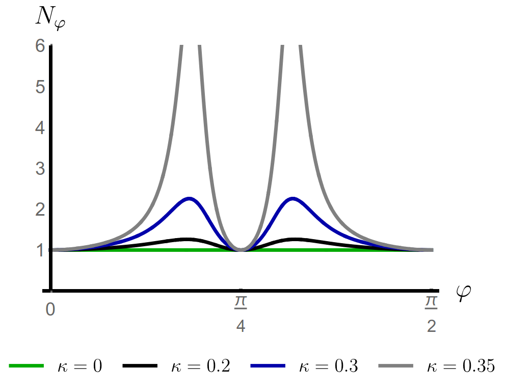
Figure 4: The scattering density as a function of the phonon direction $\varphi$, as given by Eq. (23).

Appendix C Steady-state phase diagram

The interacting Hamiltonian $H_{\mathrm{int}}$ of the two-band model contains five different types of inter-pocket and intra-pocket interactions. To study the competition between SC and SDW, these interactions are projected in the leading electronic instabilities Fernandes and Chubukov (2017). The complete phase diagram for the two-band model discussed in the main text can be obtained by solving the coupled non-linear self-consistent gap equations for the $s^{+-}$ SC gap, $\Delta=-V_{\mathrm{SC}}\sum_{\mathbf{k}}\left\langle c_{h,-\mathbf{k}\downarrow}c_{h,\mathbf{k}\uparrow}\right\rangle=V_{\mathrm{SC}}\sum_{\mathbf{k}}\left\langle c_{e,-\mathbf{k}\downarrow}c_{e,\mathbf{k}\uparrow}\right\rangle$, and the SDW order parameter $M=-V_{\mathrm{SDW}}\sum_{\mathbf{k},\sigma}\left\langle c_{h,\mathbf{k}\sigma}^{\dagger}\sigma c_{e,\mathbf{k}\sigma}\right\rangle$. Here, for convenience, all momenta are measured with respect to the center of the respective Fermi pocket: $\mathbf{K}=0$ for the hole pocket and $\mathbf{K}=\mathbf{Q}$ for the electron pocket. The equilibrium phase diagram of this model was previously calculated in Refs. Fernandes and Schmalian (2010); Vorontsov et al. (2010). Here, because we are interested in the normal-state instabilities of the system, we do not consider the full non-linear gap equations, but instead expand to cubic order in the order parameters. The reason why we need to go to cubic order instead of simply linear order is to capture the effects of the competition between SDW and SC. The coefficients of the gap equations can be obtained directly from the Ginzburg-Landau energy functional:

$$F=\frac{a_{M}}{2}M^{2}+\frac{u_{M}}{4}M^{4}+\frac{a_{\Delta}}{2}\Delta^{2}+\frac{u_{\Delta}}{4}\Delta^{4}+\frac{\gamma}{2}M^{2}\Delta^{2}\,.$$ (24)

Previously, these coefficients were computed for the two-band microscopic model in the equilibrium case Fernandes and Schmalian (2010); Vorontsov et al. (2010). Our goal here is to show that, in the non-equilibrium steady-state case, the coefficients have the same functional form, but with the Fermi-Dirac equilibrium distribution function replaced by the non-equilibrium distribution function that results from the Boltzmann equation – a procedure widely employed phenomenologically in the literature Eliashberg (1960); Eliashberg and Ivlev (1986).

To accomplish this, we use the Keldysh formalism Levchenko and Kamenev (2007); Kamenev (2011). In this case, besides the standard advanced and retarded Green’s functions, $G^{A}$ and $G^{R}$, respectively, one needs to include also the Keldysh Green’s function $G^{K}$. In situations close to equilibrium, as it is our case, the latter is related to the former by $G^{K}=f(G^{R}-G^{A})$, where $f$ is the symmetrized non-equilibrium distribution function, $f(\xi)=1-2n_{F}(\xi)$. Within the Keldysh formalism, the quadratic and quartic terms of the semi-classical energy functional Eq. (24) must be rewritten in terms of classical and quantum source components as $M^{cl}M^{q}$ ($\Delta^{cl}\Delta^{q}$) and $M^{cl}M^{cl}M^{cl}M^{q}$ ($\Delta^{cl}\Delta^{cl}\Delta^{cl}\Delta^{q}$) in order for the classical saddle point equations to be obtained via the constraints on the action $\delta S/\delta M^{q}|_{M^{q}=0}=0$ and $\delta S/\delta\Delta^{q}|_{\Delta^{q}=0}=0$. For the classical saddle point the RKA-rule applies, which implies the following causal combination of the Green’s functions in the quartic coefficients: $RRRK+RRKA+RKAA+KAAA$.

Using $\tau$-matrices for the band space and $\sigma$ for the particle-hole space, the relevant Green’s functions are expressed as:

$$\mathds{G}_{j,\alpha}^{R(K,A)}=\sum_{j,\alpha}\mathds{P}_{j,\alpha}G_{j,\alpha}^{R(K,A)}$$ (25)

where $G_{j,\alpha}^{R(A)}=\operatorname{Lim}\limits_{\delta\rightarrow 0^{+}}(\epsilon-\alpha\xi_{j}\pm i\delta)^{-1}$, $\mathds{P}_{j,\alpha}=(1+j\tau_{z})(1+\alpha\sigma_{z})/4$ and $j,\alpha\in\{+,-\}$. For convenience of notation, hereafter the hole-like band is associated with $j=-1$ and the electron-like band is associated with $j=+1$. The resulting Ginzburg-Landau coefficients are then given by:

$$a_{m}=V_{\mathrm{SDW}}-2i\mathrm{Tr}\left[\mathds{G}_{-j,\alpha}^{\mu}\tau_{x}\mathds{G}_{j,\alpha}^{\nu}\tau_{x}\right]$$ (26a)

$$a_{\Delta}=V_{\mathrm{SC}}-2i\mathrm{Tr}\left[\mathds{G}_{j,\alpha}^{\mu}\sigma_{x}\mathds{G}_{j,-\alpha}^{\nu}\sigma_{x}\right]$$ (26b)

$$u_{m}=-2i\mathrm{Tr}\left[\mathds{G}_{-j,\alpha}^{\mu}\tau_{x}\mathds{G}_{j,\alpha}^{\nu}\tau_{x}\mathds{G}_{-j,\alpha}^{\beta}\tau_{x}\mathds{G}_{j,\alpha}^{\lambda}\tau_{x}\right]$$ (26c)

$$u_{\Delta_{i}}=-2i\mathrm{Tr}\left[\mathds{G}_{j,\alpha}^{\mu}\sigma_{x}\mathds{G}_{j,-\alpha}^{\nu}\sigma_{x}\mathds{G}_{j,\alpha}^{\beta}\sigma_{x}\mathds{G}_{j,\alpha}^{\lambda}\sigma_{x}\right]$$ (26d)

$$\gamma=2i\left\{\mathrm{Tr}\left[\mathds{G}_{j,\alpha}^{\mu}\sigma_{x}\mathds{G}_{j,-\alpha}^{\nu}\sigma_{x}\mathds{G}_{j,\alpha}^{\beta}\tau_{x}\mathds{G}_{-j,\alpha}^{\lambda}\tau_{x}\right]\right.$$

$$-\left.\mathrm{Tr}\left[\mathds{G}_{j,\alpha}^{\mu}\sigma_{x}\mathds{G}_{j,-\alpha}^{\nu}\tau_{x}\mathds{G}_{-j,-\alpha}^{\beta}\sigma_{x}\mathds{G}_{-j,\alpha}^{\lambda}\tau_{x}\right]\right\}$$ (26e)

In all these expressions, the trace $\mathrm{Tr}[\ldots]$ implies summation over all indices, namely $\mathrm{Tr}[\ldots]=\sum_{j,\alpha}\int\frac{\mathrm{d}\omega}{2\pi}\int\left(\mathrm{d}p\right)\mathrm{tr}[\ldots]$, as well as the Keldysh indices (Greek letters). The summation over the latter satisfies the RKA rule, which means that for $(\mu,\nu)$, only $(R,K)$ and $(K,A)$ are involved.

In order to evaluate the quartic coefficients, it is useful to consider the generic combination of four Green’s functions:

$$\Gamma=2i\int\frac{\mathrm{d}\omega}{2\pi}\int\left(\mathrm{d}p\right)\mathrm{tr}\left[\mathds{P}_{a}\mathds{P}_{b}\mathds{P}_{c}\mathds{P}_{d}\right]\!\!\!\sum_{\begin{subarray}{c}\mu\nu\beta\lambda\\ \mathrm{RKA-Rule}\end{subarray}}\!\!\!G_{a}^{\mu}G_{b}^{\nu}G_{c}^{\beta}G_{d}^{\lambda}$$ (27)

Here, the Latin letters correspond to the combined band and particle-hole indices, whereas the Greek letters refer to Keldysh indices. Note that due to the RKA-rule, only one of the Green’s functions is a Keldysh Green’s function, as explained above. As a result, only the residue of the Keldysh Green’s function matters, since the Keldysh component is strongly peaked at the Fermi level, $\operatorname{Lim}\limits_{\delta\rightarrow 0}G_{a}^{R}-G_{a}^{A}=-2\pi i\delta(\epsilon-\xi_{a})$. If, as in our case, two of the Greens functions share the same band/particle-hole index $a$, a simple evaluation by means of a Dirac delta function is no longer possible. Instead, one can use the identities:

$$\operatorname{Lim}\limits_{\delta\rightarrow 0}2i\int\frac{\mathrm{d}\omega}{2\pi}G_{a}^{R}G_{b}^{R}G_{a}^{R}G_{b}^{K}=\\ 2\mathop{\mathrm{Re}}\operatorname{Lim}\limits_{\delta\rightarrow 0}\operatorname{Res}\limits_{G_{b}^{A},\mathrm{pole}}\left(G_{a}^{R}G_{b}^{R}G_{a}^{R}G_{b}^{A}f_{b}(\omega)\right),$$ (28a)

$$\operatorname{Lim}\limits_{\delta\rightarrow 0}2i\int\frac{\mathrm{d}\omega}{2\pi}G_{a}^{K}G_{b}^{A}G_{a}^{A}G_{b}^{A}=\\ 2\mathop{\mathrm{Re}}\operatorname{Lim}\limits_{\delta\rightarrow 0}\operatorname{Res}\limits_{G_{a}^{R},\mathrm{pole}}\left(G_{a}^{R}G_{b}^{A}G_{a}^{A}G_{b}^{A}f_{a}(\omega)\right)$$ (28b)

and for the causality-quenched configuration, accordingly:

$$\operatorname{Lim}\limits_{\delta\rightarrow 0} 2i\int\frac{\mathrm{d}\omega}{2\pi}G_{a}^{R}G_{b}^{R}G_{a}^{K}G_{b}^{A}=$$

$$2\mathop{\mathrm{Re}} \operatorname{Lim}\limits_{\delta\rightarrow 0}\left[\operatorname{Res}\limits_{G_{a}^{A},\mathrm{pole}}\left(G_{a}^{R}G_{b}^{R}G_{a}^{A}G_{b}^{A}f_{a}(\omega)\right)\right.$$

$$+\left.\operatorname{Res}\limits_{G_{b}^{R},\mathrm{pole}}\left(G_{a}^{R}G_{b}^{R}G_{a}^{R}G_{b}^{A}f_{a}(\omega)\right)\right.$$

$$-\left.\operatorname{Res}\limits_{G_{b}^{A},\mathrm{pole}}\left(G_{a}^{R}G_{b}^{R}G_{a}^{A}G_{b}^{A}f_{a}(\omega)\right)\right],$$ (29a)

$$\operatorname{Lim}\limits_{\delta\rightarrow 0} 2i\int\frac{\mathrm{d}\omega}{2\pi}G_{a}^{R}G_{b}^{K}G_{a}^{A}G_{b}^{A}=$$

$$2\mathop{\mathrm{Re}} \operatorname{Lim}\limits_{\delta\rightarrow 0}\left[\operatorname{Res}\limits_{G_{b}^{R},\mathrm{pole}}\left(G_{a}^{R}G_{b}^{R}G_{a}^{A}G_{b}^{A}f_{b}(\omega)\right)\right.$$

$$-\left.\operatorname{Res}\limits_{G_{a}^{R},\mathrm{pole}}\left(G_{a}^{R}G_{b}^{A}G_{a}^{A}G_{b}^{A}f_{b}(\omega)\right)\right.$$

$$+\left.\operatorname{Res}\limits_{G_{a}^{A},\mathrm{pole}}\left(G_{a}^{R}G_{b}^{R}G_{a}^{A}G_{b}^{A}f_{b}(\omega)\right)\right],$$ (29b)

which are derived using methods of contour integration as illustrated in Fig. 5.

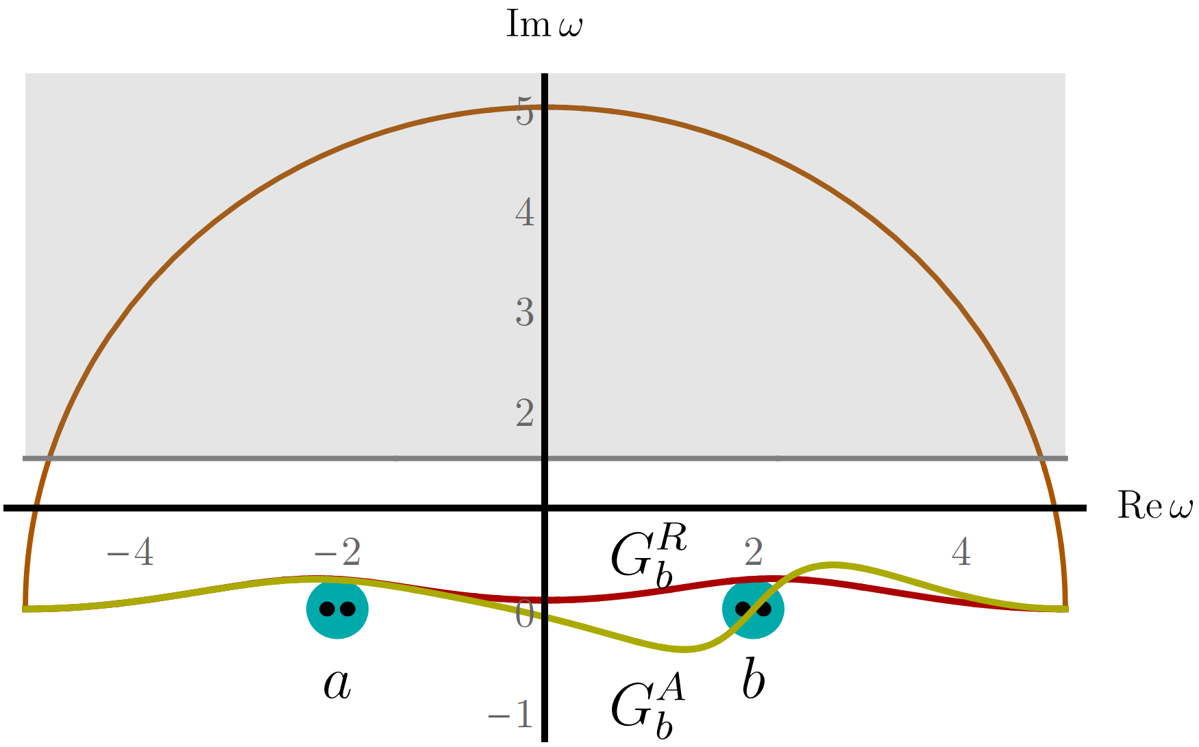
Figure 5: Illustration of the contour integration that allows to extract the relations used to determine the out of equilibrium coefficients in Eq. (28a). The gray area contains the features of the unknown function $f$ and the turquoise area corresponds to the degenerate pole, which might only be resolved by causality. As a consequence, the difference between retarded and advanced components (as typically appearing from the Keldysh Green’s function) is given by the residue of single poles or multiple poles.

As a consequence, we find the Ginzburg-Landau coefficients:

$$a_{m} =V_{\mathrm{SDW}}^{-1}-2\int\left(\mathrm{d}p\right)\frac{f_{\bar{1}}-f_{1}}{\xi_{\bar{1}}-\xi_{1}}$$ (30a)

$$a_{\Delta} =V_{\mathrm{SC}}^{-1}-\int\left(\mathrm{d}p\right)\sum_{i}\frac{f_{i}}{\xi_{i}}$$ (30b)

$$u_{m} =-\int\left(\mathrm{d}p\right)\frac{2}{\left(\xi_{\bar{1}}-\xi_{1}\right)^{2}}\left[f_{\bar{1}}^{\prime}+f_{1}^{\prime}-2\,\frac{f_{\bar{1}}-f_{1}}{\xi_{\bar{1}}-\xi_{1}}\right]$$ (30c)

$$u_{\Delta} =-\frac{1}{2}\int\left(\mathrm{d}p\right)\sum_{i}\frac{1}{\xi_{i}^{2}}\left[f_{i}^{\prime}-\frac{f_{i}}{\xi_{i}}\right]$$ (30d)

$$\gamma =\int\left(\mathrm{d}p\right)\!\frac{1}{\xi_{\bar{1}}-\xi_{1}}\left[\frac{f_{\bar{1}}}{\xi_{\bar{1}}^{2}}-\frac{f_{1}}{\xi_{1}^{2}}-\frac{f_{\bar{1}}^{\prime}}{\xi_{\bar{1}}}+\frac{f_{1}^{\prime}}{\xi_{1}}\right]$$ (30e)

where we used $\bar{1}=-1$, $f_{i}=f(\xi_{i})$, $f^{\prime}=\partial_{\xi}f(\xi)$ and $\int\left(\mathrm{d}p\right)=\int\frac{d^{2}p}{4\pi^{2}}$. In equilibrium, where $f\left(\xi\right)=\tanh\left(\frac{\beta\xi}{2}\right)$, the expressions reduce to those derived in Ref. Fernandes and Schmalian (2010).

Because the two band dispersions are parametrized by $\xi_{1}\equiv-\xi-b\left(\theta\right)$ and $\xi_{\bar{1}}=\xi$, with $b\left(\theta\right)=\delta_{\mu}+\delta_{m}\cos 2\theta$, the momentum integration can be split into an integration over momentum perpendicular to the FS ($\xi$) and momentum parallel to the FS ($\theta$), $\int\left(\mathrm{d}p\right)=N_{F}\int\frac{\mathrm{d}\theta}{2\pi}\int\mathrm{d}\xi$, where $N_{F}$ is the density of states. As a result, all the integrals over $\xi$ can be performed analytically, leaving only the angular integrals to be evaluated numerically. In terms of the Fourier components of the anisotropic temperature $\delta T_{n}$, we find:

$$a_{m} =4N_{F}\left({\,\mathrm{ln}}\frac{T}{T_{M}}-\hat{a}_{m,\mathrm{eq}}+\sum_{n}\delta\hat{a}_{m,n}\frac{\delta T_{n}}{T}\right)$$ (31a)

$$a_{\Delta} =4N_{F}\left({\,\mathrm{ln}}\frac{T}{T_{c}}+\sum_{n}\delta\hat{a}_{\Delta,n}\frac{\delta T_{n}}{T}\right)$$ (31b)

$$u_{m} =\frac{N_{F}}{T^{2}}\left(\hat{u}_{m,\mathrm{eq}}+\sum_{n}\delta\hat{u}_{m,n}\frac{\delta T_{n}}{T}\right)$$ (31c)

$$u_{\Delta} =\frac{N_{F}}{T^{2}}\left(\hat{u}_{\Delta,\mathrm{eq}}+\sum_{n}\delta\hat{u}_{\Delta,n}\frac{\delta T_{n}}{T}\right)$$ (31d)

$$\gamma =\frac{N_{F}}{T^{2}}\left(\hat{\gamma}_{\mathrm{eq}}+\sum_{n}\delta\hat{\gamma}_{n}\frac{\delta T_{n}}{T}\right)$$ (31e)

The equilibrium coefficients are given by:

$$\hat{a}_{m,\mathrm{eq}} =2(\gamma_{E}+{\,\mathrm{ln}}4)+\sum_{\alpha=\pm 1}\left\langle\psi^{(0)}(X_{\alpha})\right\rangle$$ (32a)

$$\hat{u}_{m,\mathrm{eq}} =-\frac{1}{8\pi^{2}}\sum_{\alpha=\pm 1}\left\langle\psi^{(2)}(X_{\alpha})\right\rangle$$ (32b)

$$\hat{u}_{\Delta,\mathrm{eq}} =\frac{7}{2\pi^{2}}\zeta(3)$$ (32c)

$$\hat{\gamma}_{\mathrm{eq}} =\left\langle\!\frac{\psi^{(0)}\left(\frac{1}{2}\right)}{2\pi^{2}x^{2}}\!\right\rangle-\sum_{\alpha=\pm 1}\left\langle\!\frac{\psi^{(0)}(X_{\alpha})-i\alpha\frac{x}{\pi}\psi^{(1)}(X_{\alpha})}{(2\pi x)^{2}}\!\right\rangle$$ (32d)

where we introduced the notation $x=-\frac{\delta_{\mu}}{\pi T}-\frac{\delta_{m}}{\pi T}\cos 2\theta$ and $X_{\alpha}=\frac{1}{2}+\alpha ix$; the brackets denote integration over the angular variable and $\psi^{(n)}$ is the polygamma function of order $n$. The non-equilibrium coefficients are given by:

$$\delta\hat{a}_{m,n}(x) =1-\left\langle\frac{ix}{2}\sum_{\alpha=\pm 1}\alpha\psi^{(1)}(X_{\alpha})\,\cos n\theta\right\rangle$$ (33a)

$$\delta\hat{a}_{\Delta,n} =\left\langle\cos n\theta\right\rangle=\delta_{n,0}$$ (33b)

$$\delta\hat{u}_{m,n} =-\frac{1}{32\pi^{2}}\times$$ (33c)

$$\times\sum_{\alpha=\pm 1}\left\langle\left[\psi^{(2)}(X_{\alpha})+\frac{\alpha ix}{2}\psi^{(3)}(X_{\alpha})\right]\cos n\theta\right\rangle$$ (33d)

$$\delta\hat{u}_{\Delta,n} =\frac{7}{2\pi^{2}}\zeta(3)\left\langle\cos n\theta\right\rangle=\frac{7}{2\pi^{2}}\zeta(3)\delta_{n,0}$$ (33e)

$$\delta\hat{\gamma}_{n} =-\frac{1}{8\pi^{2}}\sum_{\alpha=\pm 1}\left\langle\psi^{(2)}(X_{\alpha})\,\cos n\theta\right\rangle$$ (33f)

Note that, in the spirit of the Ginzburg-Landau approach, the temperature in the pre-factors of the quartic coefficients must be replaced by the temperature at which both transition lines meet, $T_{M}=T_{c}$. We verified that the equilibrium phase diagram resulting from these equations reproduces very well the transition lines of the phase diagram of Ref. Vorontsov et al. (2010) (including the $T_{M}$ and $T_{c}$ lines below, but in the vicinity of, the multicritical point), which used the full non-linear gap equations.

Appendix D Impact of other scattering sources

As discussed in the main text, there are two additional sources of scattering that may impact our results: impurity scattering and electron-electron scattering. These contributions can be included in the Bolztmann equation via their collision integrals:

$$I_{\mathrm{coll}}^{\mathrm{imp}}[n^{F}]=-\int\frac{\mathrm{d}^{2}p^{\prime}}{(2\pi)^{2}}\delta(\xi_{\mathbf{p}}-\xi_{\mathbf{p}^{\prime}})|M_{\mathbf{p}-\mathbf{p}^{\prime}}^{\mathrm{imp}}|^{2}\left[n_{\xi_{\mathbf{p}}}^{F}-n_{\xi_{\mathbf{p}^{\prime}}}^{F}\right]$$ (34)

$$I_{\mathrm{coll}}^{\mathrm{el-el}}[n^{F}]=-\int\frac{\mathrm{d}^{2}p^{\prime}}{(2\pi)^{2}}\int\frac{\mathrm{d}^{2}\tilde{p}}{(2\pi)^{2}}\int\frac{\mathrm{d}^{2}\tilde{p}^{\prime}}{(2\pi)^{2}}\delta(\xi_{\mathbf{p}}-\xi_{\mathbf{p}^{\prime}}+\xi_{\tilde{\mathbf{p}}}-\xi_{\tilde{\mathbf{p}}^{\prime}})\delta(\mathbf{p}-\mathbf{p}^{\prime}+\tilde{\mathbf{p}}-\tilde{\mathbf{p}}^{\prime})|M_{\mathbf{q}}^{\mathrm{el-el}}|^{2}\times\\ \times\left[n_{\xi_{\mathbf{p}}}^{F}n_{-\xi_{\mathbf{p}^{\prime}}}^{F}n_{\xi_{\tilde{\mathbf{p}}}}^{F}n_{-\xi_{\tilde{\mathbf{p}}^{\prime}}}^{F}-n_{-\xi_{\mathbf{p}}}^{F}n_{\xi_{\mathbf{p}^{\prime}}}^{F}n_{-\xi_{\tilde{\mathbf{p}}}}^{F}n_{\xi_{\tilde{\mathbf{p}}^{\prime}}}^{F}\right]$$ (35)

where $|M_{\mathbf{p}-\mathbf{p}^{\prime}}^{\mathrm{imp}}|^{2}\nu_{F}=\tau_{\mathrm{imp}}^{-1}$. To understand how these additional contributions affect the solution of the Boltzmann equation that we found, it is instructive to consider the functional form of the latter, as we did in Eq. (13). For convenience, we rewrite the functional in terms of a kernel function $K\left(h^{F}\right)$

$$\mathcal{F}\left[h^{F}\right]=\iint\frac{\mathrm{d}\theta\mathrm{d}\theta^{\prime}}{(2\pi)^{2}}N_{F}(\theta)N_{F}(\theta^{\prime})\frac{\omega_{q}|M_{\mathbf{q}}|^{2}}{4\sinh^{2}(\frac{\beta\omega_{q}}{2})}\,K\left(h^{F}\right)$$ (36)

When only non-equilibrium acoustic phonons are present, the kernel is given by:

$$K_{\mathrm{phonon}}\left(h^{F}\right) =\left(\frac{\beta\omega_{q}}{2}\right)^{2}\left[\left(\delta T_{\hat{\mathbf{p}}}+\delta T_{\hat{\mathbf{p}}^{\prime}}\right)-\tilde{h}_{q}^{B}\right]^{2}$$

$$+\frac{1}{3}\left[\pi^{2}+\left(\frac{\beta\omega_{q}}{2}\right)^{2}\right]\left(\delta T_{\hat{\mathbf{p}}}-\delta T_{\hat{\mathbf{p}}^{\prime}}\right)^{2}$$ (37)

where $\tilde{h}_{q}^{B}=2h_{q}^{B}/\beta\omega_{q}$ is proportional to the driving term. This expression is equivalent to Eq. (13), since the quadratic term in $\tilde{h}^{B}$ just provides a trivial shift of the functional.

When expressed in this form, the functional reveals in a very transparent way the competition between two opposing effects, represented by the two positive-defined terms of the kernel. The first term, arising from the driving of the acoustic phonons, is minimized by setting an anisotropic effective temperature profile $\left(\delta T_{\hat{\mathbf{p}}}+\delta T_{\hat{\mathbf{p}}^{\prime}}\right)=\tilde{h}_{q}^{B}$. The second term, on the other hand, corresponds to the relaxation of the electrons back to a uniform temperature profile, since this term is minimized by $\delta T_{\hat{\mathbf{p}}}-\delta T_{\hat{\mathbf{p}}^{\prime}}=0$. By comparing the coefficients of this term, it is clear that as long as $\frac{\beta\omega_{q}}{2}\gtrsim\pi$, both terms are comparable. In the case where $\frac{\beta\omega_{q}}{2}\lesssim\pi$, the second term dominates, and the effective temperature profile is expected to become less anisotropic. This is precisely what we note from our numerical results shown in Fig. 2c of the main text: when $\Omega_{0}\equiv\frac{\beta\omega_{0}}{2}$ decreases towards $1$, the ratio $\delta T(\frac{\pi}{4})/\delta T(0)$ also decreases.

This qualitative analysis can be extended to include the effects of impurity scattering and electron-electron scattering. The impurity collision integral shown in Eq. (34) gives rise to the following functional kernel:

$$K_{\mathrm{imp}}\left(h^{F}\right)=\frac{|M^{\mathrm{imp}}|^{2}}{|M(\hat{\mathbf{q}})|^{2}}\frac{4\sinh^{2}(\beta\omega_{q}/2)}{\beta\omega_{q}}\frac{\pi^{2}}{3}\left(\delta T_{\hat{\mathbf{p}}}-\delta T_{\hat{\mathbf{p}}^{\prime}}\right)^{2}$$ (38)

It is clear that impurity scattering favors a uniform effective temperature profile, adding up to the second term of the phonon kernel in Eq. (37). Thus, for the first term of $K_{\mathrm{phonon}}$ to be comparable to these terms, the following condition has to be met:

$$\left(\frac{\beta\omega_{q}}{2}\right)^{2}\gtrsim\pi^{2}+4\pi^{2}\frac{|M^{\mathrm{imp}}|^{2}}{|M(\hat{\mathbf{q}})|^{2}}\frac{\sinh^{2}(\beta\omega_{q}/2)}{\beta\omega_{q}}$$ (39)

Thus, for temperatures comparable to the energy of the excited phonon mode, $T\sim\omega_{0}$, the anisotropic temperature profile resulting from the minimization of the functional would persist even if the impurity and phonon matrix elements are of the same order. Of course, as temperature becomes much smaller than $\omega_{0}$, the effect will only persist if $\left|M^{\mathrm{imp}}\right|^{2}\ll\left|M(\hat{\mathbf{q}})\right|^{2}$. There are basically two different scenarios in which this condition is satisfied. The first is when the system is clean, since $|M^{\mathrm{imp}}|^{2}$ scales with the impurity concentration. The second is when the sound velocity $v_{s}$ of the system is small, which makes $\left|M(\hat{\mathbf{q}})\right|^{2}$ large.

The impact of the electron-electron scattering, described by the collision integral (35), is more subtle. First, one has to distinguish energy relaxation and momentum relaxation processes. As discussed in the main text, the former is expected to be faster than the latter, particularly in two-dimensional systems. It is the energy relaxation that leads to a rather quick thermalization of the electronic degrees of freedom; however, this process does not smear out the anisotropic effective temperature caused by the non-equilibrium phonons, as it is not capable of relaxing momentum. On the contrary, this process actually helps to establish the anisotropic effective temperature, as it enforces the electronic distribution to be nearly thermal, as we tacitly assumed when we linearized the Boltzmann equation.

Momentum relaxation due to electron-electron scattering, on the other hand, has the potential to wash away the anisotropy in the temperature. To estimate this effect, we recast the collision integral Eq. (35) in a functional form. The form of the functional, however, is different than that of Eq. (36), because it involves four electronic states. Generally, the functional is given by

$$\iint\frac{\mathrm{d}\theta\mathrm{d}\theta^{\prime}}{(2\pi)^{2}}N(\theta)N(\theta^{\prime})\iint\frac{\mathrm{d}\tilde{\theta}\mathrm{d}\tilde{\theta}^{\prime}}{(2\pi)^{2}}N(\tilde{\theta})N(\tilde{\theta}^{\prime})\frac{(\beta\omega_{q})^{2}|M_{\mathbf{q}}^{\mathrm{el-el}}|^{2}}{4\sinh^{2}(\beta\omega_{q}/2)}\left[\frac{1}{3}\left(\pi^{2}+\frac{1}{2}\beta^{2}\omega_{q}^{2}\right)\left(\left(\delta T_{\hat{\mathbf{p}}}-\delta T_{\hat{\mathbf{p}}^{\prime}}\right)^{2}+\left(\delta T_{\hat{\tilde{\mathbf{p}}}}-\delta T_{\hat{\tilde{\mathbf{p}}}^{\prime}}\right)^{2}\right)\right.\\ \left.+\left(\frac{\beta\omega_{q}}{2}\right)^{2}\left(\left(\delta T_{\hat{\mathbf{p}}}-\delta T_{\hat{\tilde{\mathbf{p}}}}\right)^{2}+\left(\delta T_{\hat{\mathbf{p}}}-\delta T_{\hat{\tilde{\mathbf{p}}}^{\prime}}\right)^{2}+\left(\delta T_{\hat{\mathbf{p}}^{\prime}}-\delta T_{\hat{\tilde{\mathbf{p}}}}\right)^{2}+\left(\delta T_{\hat{\mathbf{p}}^{\prime}}-\delta T_{\hat{\tilde{\mathbf{p}}}^{\prime}}\right)^{2}\right)\right]$$ (40)

If we attempt to recast this functional in the form given by Eq. (36), we have to integrate out the momenta $\tilde{\theta}$ and $\tilde{\theta}^{\prime}$, which will generate non-linear effects. For simplicity, if we focus only on the first term, and cast it in the form of Eq. 36, we find the following kernel:

$$K^{\mathrm{el-el}}\left(h^{F}\right) =\frac{|M_{\mathbf{q}}^{\mathrm{el-el}}|^{2}}{|M(\hat{\mathbf{q}})|^{2}}\nu_{F}^{2}\beta\omega_{q}$$

$$\times\frac{1}{3}\left(\pi^{2}+\frac{1}{2}\beta^{2}\omega_{q}^{2}\right)\left(\delta T_{\hat{\mathbf{p}}}-\delta T_{\hat{\mathbf{p}}^{\prime}}\right)^{2}$$ (41)

Thus, for $T\sim\omega_{0}$, this term does not significantly enhance the corresponding term of the phononic kernel, Eq. (37), provided that $|M_{\mathbf{q}}^{\mathrm{el-el}}|^{2}\nu_{F}^{2}$ is of the same order as $|M(\hat{\mathbf{q}})|^{2}$. As in the case of impurities, the phononic contribution $|M(\hat{\mathbf{q}})|^{2}$ will be enhanced in systems near a structural transition.