The population of SNe/SNRs in the starburst galaxy Arp 220

Abstract

Context. The nearby ultra-luminous infrared galaxy (ULIRG) Arp 220 is an excellent laboratory for studies of extreme astrophysical environments. For 20 years, Very Long Baseline Interferometry (VLBI) has been used to monitor a population of compact sources thought to be supernovae (SNe), supernova remnants (SNRs), and possibly active galactic nuclei (AGNs). SNe and SNRs are thought to be the sites of relativistic particle acceleration powering star formation induced radio emission in galaxies, and are hence important for studies of for example the origin of the FIR-radio correlation.

Aims. In this work we aim for a self-consistent analysis of a large collection of Arp 220 continuum VLBI data sets. With more data and improved consistency in calibration and imaging, we aim to detect more sources and improve source classifications with respect to previous studies. Furthermore, we aim to increase the number of sources with robust size estimates, to analyse the compact source luminosity function (LF), and to search for a luminosity-diameter (LD) relation within Arp 220.

Methods. Using new and archival VLBI data spanning 20 years, we obtained 23 high-resolution radio images of Arp 220 at wavelengths from 18 cm to 2 cm. From model-fitting to the images we obtained estimates of flux densities and sizes of detected sources. The sources were classified in groups according to their observed lightcurves, spectra and sizes. We fitted a multi-frequency supernova light-curve model to the object brightest at 6 cm to estimate explosion properties for this object.

Results. We detect radio continuum emission from 97 compact sources and present flux densities and sizes for all analysed observation epochs. The positions of the sources trace the star forming disks of the two nuclei known from lower-resolution studies. We find evidence for a LD-relation within Arp 220, with larger sources being less luminous. We find a compact source LF $n(L)\propto L^{\beta}$ with $\beta=-2.19\pm 0.15$, similar to SNRs in normal galaxies, and we argue that there are many relatively large and weak sources below our detection threshold. The brightest (at 6 cm) object 0.2195+0.492 is modelled as a radio SN with an unusually long 6 cm rise time of 17 years.

Conclusions. The observations can be explained by a mixed population of SNe and SNRs, where the former expand in a dense circumstellar medium (CSM) and the latter interact with the surrounding interstellar medium (ISM). Nine sources are likely luminous SNe, for example type IIn, and correspond to few percent of the total number of SNe in Arp 220. Assuming all IIns reach these luminosities, and no confusion with other SNe types, our data are consistent with a total SN-rate of 4 yr^-1 as inferred from the total radio emission given a normal stellar initial mass function (IMF). Based on the fitted luminosity function, we argue that emission from all compact sources, also below our detection threshold, make up at most 20% of the total radio emission at GHz frequencies. However, colliding SN shocks and the production of secondary electrons through cosmic ray (CR) protons colliding with the dense ISM may cause weak sources to radiate much longer than assumed in this work. This could potentially explain the remaining fraction of the smooth synchrotron component. Future, deeper observations of Arp 220 will probe the sources with lower luminosities and larger sizes. This will further constrain the evolution of SNe/SNRs in extreme environments and the presence of AGN activity.

1 Introduction

The ultra luminous infrared galaxy (ULIRG) Arp 220 (Arp, 1966) is a merging system with two nuclei (east and west) about 1^′′ (370 pc) apart (Norris, 1988). The nuclei are hosts of intense star formation (for example Parra et al. 2007) as well as possible active galactic nuclei (AGN) activity (Downes & Eckart, 2007). Arp 220 has been subject of global very long baseline interferometry (VLBI) monitoring for 20 years, starting with the discovery of multiple compact (¡1pc) sources by Smith et al. (1998b) at 18 cm. Subsequent observations revealed approximately 50 sources thought to be a radio supernovae (SNe) and/or supernova remnants (SNRs), with many sources seen at multiple wavelengths (Rovilos et al., 2005; Lonsdale et al., 2006; Parra et al., 2007; Batejat et al., 2011, 2012).

Multiple sources in Arp 220 were resolved by Batejat et al. (2011) and shown to be consistent with a luminosity-diameter (LD) relation of $L\propto D^{-9/4}$ when extrapolating from the lower density galaxies LMC and M82. The data presented by Batejat et al. (2011) were however not sensitive enough to determine an LD-relation within Arp 220 itself. Evidence for possible variability in three sources was presented by Batejat et al. (2012), but these sources are very weak, and multiple sensitive observing epochs are required to determine the nature of the apparent variability.

With its large population of SNe/SNRs in a very dense ISM ($\sim 10^{5}$ cm^-3; Scoville et al. (2015)) with strong (mGauss) magnetic fields (Lacki & Beck, 2013; Yoast-Hull et al., 2016), Arp 220 is an excellent laboratory to study the physics of star formation in extreme environments. SNe and SNRs are also the sources of relativistic particles which are responsible for the star formation induced synchrotron radio emission in galaxies. Observational constraints on how SNe interact with a dense ISM may provide useful input to theories seeking to explain the well known FIR-radio correlation. Furthermore, the SNe blast waves are thought to be important for stellar feedback in galaxies, since they provide the driving force behind the large scale winds observed from dense starburst regions such as M 82.

The focus of this paper is to present a self-consistent set of data for the compact objects in Arp 220. We present both new and previously published data at multiple frequencies spanning 20 years. The new observations were designed to (1) improve our understanding of the evolutionary status of the SNe/SNRs, (2) investigate the LD-relation within Arp 220, (3) determine the nature of the variable sources. In addition to new data, archival data was re-analysed using similar calibration and imaging strategies to allow intercomparison. This paper presents the full data set and discusses the general properties of the population of compact objects. In future papers we intend to model in detail individual objects and the overall population of compact sources to constrain the evolutionary history of the compact radio objects.

This paper is organised as follows. In Sect. 2 we describe the observations as well as the method used to extract flux densities and sizes from the observed data. In Sect. 3 we present the results of our analysis. These results are discussed in Sect. 4 focusing on the statistical properties of the source population rather than individual objects. Finally, we summarise our conclusions and future work in Sect. 5.

Throughout this paper we have assumed an angular size distance to Arp 220 of 77 Mpc, that is 1 mas=0.37 pc, and luminosity distance of 80 Mpc, as obtained from Wright (2006) (with $H_{0}=69.9$, $\Omega_{M}$=0.286 and $\Omega_{\mathrm{vac}}=0.714$) using $cz=5469$ km/s (de Vaucouleurs et al., 1991). All spectral indices $\alpha$ assume the flux density follows $S_{\nu}\propto\nu^{+\alpha}$.

2 Observations and data reduction

This paper presents data from 23 VLBI epochs at wavelengths from 18 to 2 cm, see Table 1, spanning 20 years. Nine of these data sets have not been published before. All data were processed into final images starting from the archival raw data. Most observations were performed with global VLBI using typically 15-20 antennas all over the world, including the VLBA and the EVN. The experiments GC031, BB297 and BB335 included multiple observations spanning a few months, the purpose being to look for short term variability. We note, however, that the epochs BB297B and BB297C were severely limited in sensitivity due to lack of fringes to multiple antennas, and therefore their respective 18 cm and 3.6 cm epochs (which are the least sensitive) have been excluded from the analysis in this paper.

All calibration and imaging was performed using the 31DEC16 release of the Astronomical Image Processing System (AIPS) (Greisen, 2003) from the National Radio Astronomy Observatory (NRAO). The full reduction process, from loading of data to final images, was scripted for all data sets using the Python-based interface to AIPS, ParselTongue (Kettenis et al., 2006) 2.3. All the scripts are available via the CDS as described in appendix A. A general description of the calibration strategy employed can be found in Appendix B. The interested reader may find all details, such as task parameters, in the ParselTongue scripts. Furthermore, all the FITS images obtained when running the calibration and imaging scripts, that is two images (east and west nuclei) of each of the 23 experiments listed in Table 1, which are the basis of the analysis presented in this paper, are also available via the CDS as described in appendix A.

Table 1: List of the 23 observations processed and analysed in this work. The RMS noise was measured in source free regions of the map, as noted in Sect. 2.3.

Exp.	Obs. date	$\lambda$	Beam	Beam position	Image RMS
	YYYY-MM-DD	(cm)	(mas)	angle [deg]	($\mu$Jy/beam)
GL015	1994-11-13	18.1	8.2x2.5	-9.2	36
GL021	1997-09-15	18.2	8.4x2.8	-8.7	40
GL026	2002-11-16	18.2	6.4x2.9	-16.5	12
GD017A	2003-11-09	18.2	6.7x2.8	-18.3	11
GD017B	2005-03-06	18.2	6.2x3.1	-15.7	15
BP129	2006-01-09	13.3	6.4x3.5	-3.7	173
BP129	2006-01-09	6.0	2.7x1.4	0.1	100
BP129	2006-01-09	3.6	1.8x0.9	0.1	91
GD021A	2006-06-06	18.2	6.6x2.9	-21.9	16
GC028	2006-11-28	3.6	1.4x0.5	-10.4	39
GC028	2006-12-28	2.0	1.4x0.4	-13.0	25
GC031A	2008-06-10	6.0	2.2x0.8	-13.2	17
GC031B	2008-10-24	6.0	1.9x0.8	-17.6	13
GC031C	2009-02-27	6.0	2.0x0.8	-17.6	13
BB297A	2011-05-16	18.2	10.8x4.0	-16.6	40
BB297A	2011-05-16	6.0	2.1x1.0	-13.4	16
BB297A	2011-05-16	3.6	1.6x0.5	-6.5	30
BB297B	2011-05-17	6.0	3.0x0.8	-16.1	32
BB297C	2011-06-11	6.0	2.7x1.0	29.2	33
BB335A	2014-08-01	6.0	3.0x0.9	-9.8	9
BB335A	2014-08-01	3.6	1.9x0.6	-5.0	17
BB335B	2014-10-13	6.0	3.2x1.0	-11.0	10
BB335B	2014-10-13	3.6	1.8x0.6	-5.5	19

We note that in this paper we sometimes use the letters L, S, C, X and U to designate frequency bands, similar to the IEEE standard letter designations for radar frequency bands (IEEE Std 521-2002). Table 2 provides a quick reference for translation between the letters used in this paper and the approximate central wavelength of observations. We note that the central observing wavelength is listed for each observation in Table 1.

Table 2: Frequency band letter designations used in this paper.

Band	Obs. wavelength
L	18 cm
S	13 cm
C	6 cm
X	3.6 cm
U	2 cm

Previous studies of Arp 220 have used different (although similar) methods to analyse the data. For example, different criteria have been used to determine the catalogue of sources to analyse. In the following subsections we describe how we form a source catalogue, how we fit sizes and flux densities and estimate the corresponding uncertainties, and how we obtain more robust size-estimates by averaging measurements close in time.

2.1 Building a source catalogue

To increase our sensitivity for source detection we average all 6 cm images together, as a simple weighted average where each image was weighted by its RMS noise given in Table 1, to the power of $-2$. By such averaging, we obtain the deepest maps yet (off-source RMS noise $\sigma=4.3\,\mu$Jy/beam) of the two nuclei. The central parts of these two stacked images are presented in Fig. 1.

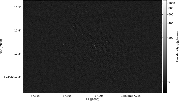
(a) The eastern nucleus of Arp 220

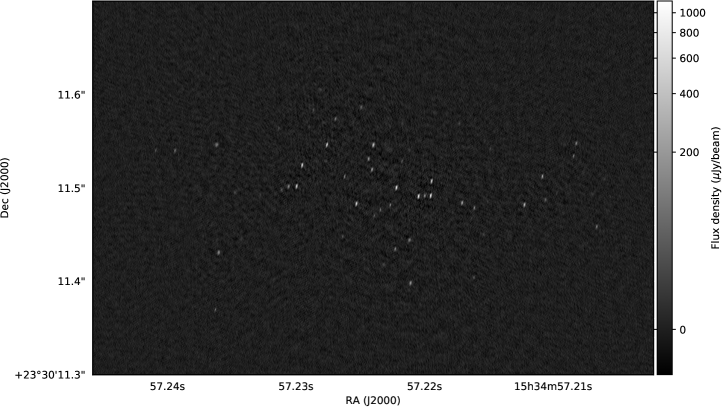
(b) The western nucleus of Arp 220

Figure 1: Cutouts of the central parts of the stacked 6 cm images towards the east and west nuclei of Arp 220, with off-source RMS noise $\sigma=4\mu$Jy beam^-1. The two panels are displayed using the same arcsinh grey-scale from $-20\mu$Jy beam^-1 ($-5\sigma$) to $1140\mu$Jy beam^-1 (the maximum brightness value). The full $0.8192^{\prime\prime}\times 0.8192^{\prime\prime}$ images of both nuclei were used for the source finding, as described in Sect. 2.1. The positions of the sources studied in this work is shown in Fig. 3.

To produce a source catalogue we apply the source finding software PyBDSM version 1.8.6 (Mohan & Rafferty, 2015) on the stacked image, with a threshold of six times the (stacked) image RMS noise, resulting in a catalogue of 75 sources at 6 cm. Similarly, we stacked the 18 cm and 3.6 cm images (stacked sensitivities of 5 and 10$\mu$Jy/beam respectively) and detected 22 additional sources seen only at 18 cm (no new additions were found in the 3.6 cm images). The total catalogue hence contains 97 sources and is presented in Tables 3 and 4. We note that three additional sources were detected in OH-maser emission only, that is no continuum, as briefly discussed in Appendix E.4.1. The maser channels in the data were however excluded when making the FITS images analysed in this paper.

To estimate the expected number of false positives we use a beam of major and minor FWHM 3 mas and 1 mas respectively (similar to the most sensitive epochs which have the largest impact on the weighted average). Given the number of independent beam elements searched across the two nuclei, a threshold of $6\sigma$ implies an expected number of false positives of $6\cdot 10^{-4}$, that is well below one. We note that lowering the threshold to $5\sigma$ would give one expected false detection.

2.2 Fitting source sizes and flux densities

In principle, it is best to fit models directly to the calibrated visibilities, instead of the cleaned images, to avoid any effects introduced by deconvolution (for exampleMartí-Vidal et al. 2014). However, the number of sources in Arp 220, which need to be fitted simultaneously in the Fourier domain, make visibility fitting impractical. We therefore decided to fit models to the cleaned images. All sources were assumed to be optically thin shells with a fractional shell width of 30%, similar to the value observed for SN1993J (see for example Martí-Vidal et al. 2011). The fitting was done using the bounded least-squares algorithm implemented in the Python package SciPy . More details and examples of fitting results are presented in Appendix C. A comparison of the results obtained in this work with previous published values using the same data is presented in Appendix E. We note that although we fit sizes at all wavelengths, the angular resolution at 18 cm and 13 cm is not sufficient to obtain meaningful sizes at these wavelengths.

2.3 Uncertainties

Based on the observed scatter of the fitted positions (see Appendix E.2), we estimate that the catalogue positions given in Tables 3 and 4 are accurate to within $\pm 1$ mas. For flux densities we estimate the uncertainty as

$$E_{f}=\sqrt{(3\sigma)^{2}+(0.1F)^{2}}$$ (1)

where $\sigma$ is the map RMS and $F$ is the measured flux density. This includes both a conservative estimate of the image noise effects, as well a 10% uncertainty on the absolute flux density calibration. Finally, for source sizes, we adopt an uncertainty based on Eq.7 by Martí-Vidal et al. (2012) of

$$E_{s}=3b_{\text{maj}}/\sqrt{\text{STN}}$$ (2)

where $b_{\text{maj}}$ is the major axis of the fitted CLEAN beam, and STN is the signal-to-noise ratio defined as $F$ divided by the respective map RMS noise. We find the uncertainties calculated above to reflect well the observed scatter in simulated data, see Appendix C.

We note that the RMS values given in Table 1 are measured in source-free regions of the map. Specifically, the RMS is measured from the leftmost 128x8192 pixels of each 8192x8192 pixel image of the western nucleus. We quote these RMS values because the source-free regions measure the performance of the instrument, that is telescope sensitivity, rather than imaging limitations. Hence, the off-source RMS is a good way to compare the different observing epochs. We acknowledge that the RMS in the central regions of the nuclei are generally higher, due to residual sidelobes from imperfect calibration and/or imaging as well as sources just below our detection threshold. This is the reason we use $3\sigma$ in for example Eq. 1 rather than just $1\sigma$ (as used by multiple previous studies analysing parts of these data).

2.4 Averaging of multiple epochs

Although we fit source flux densities and sizes at each epoch separately, the uncertainties are sometimes very large, in particular on the sizes of the weakest sources. We therefore, in some sections of this paper, calculate and discuss average sizes and flux densities using measurements from multiple epochs. An average size is calculated as the weighted average

$$\bar{s}=\frac{\sum s_{i}/E_{s_{i}}^{2}}{\sum 1/E_{s_{i}}^{2}}$$ (3)

where the uncertainty of the weighted mean is calculated as

$$\bar{E}_{s}=\frac{1}{\sqrt{\sum 1/E_{s_{i}}^{2}}}$$ (4)

where $s_{i}$ is a size fitted from an image and $E_{s_{i}}$ is the corresponding uncertainty according to Eq. 2. An average flux density is calculated in the same way, using the measured flux densities and their respective uncertainties instead of the sizes in Eqns. 3 and 4.

2.5 Source classification

To facilitate a discussion of the data, we classified all sources in three groups based on their 6 cm evolution between the experiments GC031 and BB335. The sources were labelled either Rise, Fall, or Slowly varying (abbreviated S-var in many places in this paper) according to the following criteria. First, average flux densities and flux density uncertainties were calculated (as described in Sect. 2.4) for the GC031 and BB335 experiments, so that we obtained two flux density values per source. Let now $F_{\mathrm{GC}}$ and $E_{\mathrm{GC}}$ be the average flux density and flux density uncertainty for a given source obtained for the GC031 experiment, and $F_{\mathrm{BB}}$ and $E_{\mathrm{BB}}$ be the corresponding values for the BB335 experiment. A source was classified as Rise if $(F_{\mathrm{GC}}+E_{\mathrm{GC}})<0.9\times(F_{\mathrm{BB}}-E_{\mathrm{BB}})$ and as Fall if $(F_{\mathrm{GC}}-E_{\mathrm{GC}})>1.1\times(F_{\mathrm{BB}}+E_{\mathrm{BB}})$. If none of these conditions were satisfied, that is if there was no strong 6 cm evidence that a source was increasing or decreasing, the source was classified as Slowly varying with respect to the noise. We note that weak sources in the S-var category are not ruled out from increasing or decreasing by more than 10%, but there is no positive evidence for such variations given the measured uncertainties. A few sources were not detected in either GC031 or BB335 and are hence labelled N/A in Tables 3 and 4.

2.5.1 Motivation

Note the classification presented in Sect. 2.5 is purely observational: it does not imply any particular source nature (such as SNe/SNRs). A detailed interpretation of the nature of the sources should of course use all the available information. One may therefore ask why we decided to base the classification only on the 6 cm lightcurves? There are multiple reasons for this choice.

The purpose of this classification is to facilitate the discussion. However, we find it instructive to divide the sources in groups already for the presentation of the results in Sect. 3. Given the number of sources and the high level of detail in these data, a physical classification (in contrast to this observational one) requires an extensive discussion to motivate the different possible classes. Such a discussion would be out of place before all the results are presented.

One may argue that if one devises classifications solely based on one waveband, one should use 18 cm since it spans the longest period in time. However, the 18 cm behaviour varies considerably between sources which have similar trends at 6 cm. Indeed, multiple studies (for example Smith et al. 1998a; Lonsdale et al. 2006; Varenius et al. 2016) argue that free-free absorption may significantly impact the flux densities measured at 1.4 GHz, which indicate that a classification based on 18 cm lightcurves may not reflect intrinsic source properties. Finally, the 18 cm observations do not have enough angular resolution to properly disentangle the emission of all sources, as a few sources are very close, thus mixing the lightcurves of blended sources.

In principle, also the 6 cm measurements may be affected by free-free absorption, and therefore one should use the 3.6 cm measurements to classify sources based on intrinsic properties. However, given the available data, we find the 6 cm observations to provide more robust lightcurves. The reason for this is twofold: first, the 6 cm observations are, in general, more sensitive than the 3.6 cm observations. Second, although the recent 3.6 cm observations in experiment BB335 reach a relatively high sensitivity, we lack an experiment with comparable sensitivity far back in time. At 6 cm we have the experiments GC031 and BB335, both with high sensitivity, separated by about 6 years in time. Given the above arguments, we decided to use the 6 cm lightcurves as the basis of our classification. We find that these simple classes provide an excellent foundation for the presentation of results and subsequent discussion of the data. We note that the physical nature of the sources is discussed in Sect. 4.

3 Results

We detect 97 compact continuum sources in Arp 220 with positions given in Tables 3 and 4. The sources show a variety of lightcurves, spectra and sizes. A comprehensive summary of all data available for each source is presented in Appendix F. In this appendix, all measured flux densities and sizes are plotted as function of time for all sources. An approximate spectrum is also shown for each source. Note that all measured flux densities and sizes are also available in machine-readable format via CDS as described in appendix A. The diameters and corresponding uncertainties listed in Tables 3 and 4 are calculated using Eqs. 3 and 4 from sizes fitted in the four images obtained at 6 cm and 3.6 cm in experiments BB335A and BB335B.

The sources were classified as described in Sect. 2.5. Examples of sources in the three categories Rise, Fall, and Slowly varying (or S-var) are shown in Fig. 2. For the purpose of the discussion we show two sources for each class to illustrate the variations in multi-frequency lightcurves within the classes.

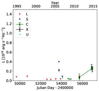
(a) Rise (0.2262+0.512)

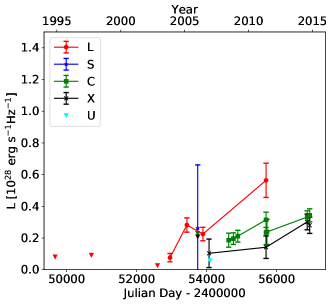
(b) Rise (0.2108+0.512)

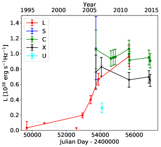
(c) Slowly varying (S-var) (0.2195+0.492)

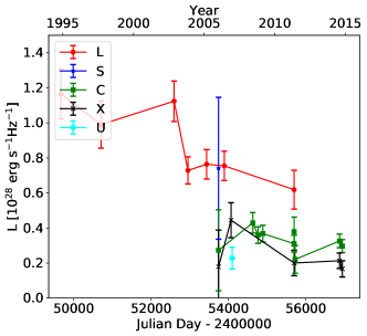
(d) Slowly varying (S-var) (0.2171+0.484)

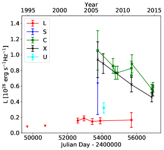
(e) Fall (0.2253+0.483)

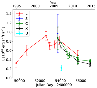
(f) Fall (0.2122+0.482)

Figure 2: Lightcurves to illustrate the source classifications Rise, Slowly varying (or S-var) and Fall used in this paper. For the purpose of the discussion, two sources are shown for each class, to show the differences in multi-frequency behaviour within the classes. All panels have the same scale for easy comparison. The horizontal axis below the panels show time in Julian Days, while the horizontal axis on top of the panels show the time in decimal years. In Sect. 4.3 we argue that these lightcurves are consistent with SNe/SNRs in different evolutionary stages, where the approximate time order corresponds to panels a, c, f, b, d. Panel e may represent a stage similar to f but with significant free-free absorption. Note that the label L on the vertical axis here denotes spectral luminosity.

Table 3: List of the 45 sources analysed in this work in the eastern nucleus. $\Delta$R.A. and $\Delta$Dec. are given with respect to the position R.A. 15^h34^m57.0000^s and Dec. 23^∘30^′11.000^′′. Flux densities F${}_{\mathrm{6\,cm}}$ are measured by fitting a spherical shell to BB335B. Average diameters calculated according to Sect. 2.4 from the 3.6 cm and 6 cm measurements in experiments BB335A and BB335B.

$\Delta$R.A. [s]	$\Delta$Dec. [′′]	Legacy name	Class	F${}_{\mathrm{6\,cm}}$ [$\mu$Jy]	Average diameter [mas]
0.2758	0.276	E22	Rise	$128\pm 30$	$5.06\pm 1.31$
0.2789	0.293	E21	S-var	$109\pm 29$	$3.21\pm 2.17$
0.2801	0.353		S-var	$49\pm 28$	$3.84\pm 4.18$
0.2814	0.316		S-var	$68\pm 28$	$2.00\pm 2.41$
0.2821	0.183	E20	S-var	$181\pm 33$	$3.03\pm 1.21$
0.2835	0.308		Rise	$116\pm 30$	$3.72\pm 2.04$
0.2840	0.151	E19	S-var	$<27$	$2.62\pm 3.39$
0.2842	0.226	E18	S-var	$104\pm 29$	$2.00\pm 1.91$
0.2848	0.294		Fall	$77\pm 28$	$1.29\pm 2.74$
0.2848	0.471	E16	Fall	$94\pm 29$	$2.75\pm 1.36$
0.2850	0.193	E17	Fall	$107\pm 29$	$2.70\pm 2.37$
0.2858	0.013		S-var	$<27$	N/A
0.2868	0.297	E14	S-var	$553\pm 61$	$0.87\pm 0.53$
0.2875	0.352		Fall	$121\pm 30$	$2.57\pm 0.80$
0.2878	0.308	E13	Fall	$184\pm 33$	$3.03\pm 1.12$
0.2881	0.369		Rise	$156\pm 31$	$0.78\pm 1.06$
0.2883	0.338		S-var	$110\pm 29$	$1.83\pm 0.94$
0.2887	0.201		S-var	$166\pm 32$	$1.01\pm 0.98$
0.2890	0.337		S-var	$115\pm 30$	$0.97\pm 1.12$
0.2891	0.253		S-var	$123\pm 30$	$3.13\pm 1.27$
0.2897	0.278		S-var	$97\pm 29$	$2.16\pm 1.95$
0.2897	0.335		S-var	$172\pm 32$	$1.48\pm 0.80$
0.2910	0.325	E11	S-var	$180\pm 33$	$1.77\pm 0.86$
0.2914	0.333		Fall	$216\pm 35$	$0.98\pm 0.80$
0.2915	0.335	E10	Fall	$853\pm 89$	$0.56\pm 0.40$
0.2915	0.476	E9	S-var	$43\pm 28$	$0.97\pm 4.50$
0.2919	0.340		S-var	$93\pm 29$	$1.63\pm 1.30$
0.2928	0.373	E24	S-var	$286\pm 39$	$1.34\pm 0.68$
0.2931	0.330	E8	S-var	$73\pm 28$	$0.44\pm 2.40$
0.2938	0.344		Fall	$<27$	$2.74\pm 1.25$
0.2940	0.481		S-var	$125\pm 30$	$3.86\pm 1.88$
0.2943	0.279	E7	S-var	$127\pm 30$	$2.22\pm 1.48$
0.2947	0.263	E6	S-var	$74\pm 28$	$1.85\pm 2.18$
0.2951	0.384		Rise	$215\pm 35$	$0.86\pm 0.94$
0.2954	0.393		S-var	$122\pm 30$	$3.07\pm 1.91$
0.2959	0.263		S-var	$89\pm 29$	$2.84\pm 2.38$
0.2971	0.378		S-var	$63\pm 28$	$3.14\pm 0.95$
0.2979	0.419	E5	S-var	$137\pm 30$	$1.89\pm 0.87$
0.2995	0.502		S-var	$54\pm 28$	$0.67\pm 1.78$
0.3011	0.341		Rise	$312\pm 41$	$0.51\pm 0.68$
0.3073	0.332	E3	Rise	$80\pm 28$	$1.80\pm 2.49$
0.3073	0.456		N/A	$<27$	N/A
0.3090	0.618		N/A	$<27$	N/A
0.3103	0.575		N/A	$<27$	N/A
0.3125	0.494		N/A	$<27$	N/A

Table 4: List of the 52 sources analysed in this work in the western nucleus. $\Delta$R.A. and $\Delta$Dec. are given with respect to the position R.A. 15^h34^m57.0000^s and Dec. 23^∘30^′11.000^′′. Flux densities F${}_{\mathrm{6\,cm}}$ are measured by fitting a spherical shell to BB335B. Average diameters calculated according to Sect. 2.4 from the 3.6 cm and 6 cm measurements in experiments BB335A and BB335B.

$\Delta$R.A. [s]	$\Delta$Dec. [′′]	Legacy name	Class	F${}_{\mathrm{6\,cm}}$ [$\mu$Jy]	Average diameter [mas]
0.2066	0.458	W46	S-var	$235\pm 37$	$2.00\pm 0.86$
0.2082	0.548	W44	S-var	$267\pm 39$	$1.60\pm 0.82$
0.2084	0.534		Rise	$197\pm 34$	$0.61\pm 0.92$
0.2106	0.487		S-var	$167\pm 33$	$2.08\pm 0.95$
0.2108	0.512		Rise	$448\pm 53$	$0.88\pm 0.64$
0.2122	0.482	W42	Fall	$485\pm 56$	$1.20\pm 0.61$
0.2149	0.542		S-var	$83\pm 29$	$0.79\pm 1.66$
0.2154	0.450		S-var	$77\pm 29$	$2.33\pm 2.32$
0.2161	0.479	W40	S-var	$225\pm 36$	$1.15\pm 0.86$
0.2162	0.404	W41	S-var	$112\pm 30$	$1.86\pm 1.46$
0.2171	0.484	W39	S-var	$387\pm 48$	$1.44\pm 0.73$
0.2173	0.569		Fall	$89\pm 30$	$2.90\pm 1.16$
0.2194	0.507	W58	Rise	$820\pm 86$	$0.58\pm 0.51$
0.2195	0.492	W34	S-var	$1185\pm 122$	$0.51\pm 0.40$
0.2200	0.492	W33	Fall	$173\pm 33$	$2.37\pm 1.00$
0.2205	0.491	W56	S-var	$1073\pm 111$	$0.72\pm 0.40$
0.2211	0.398	W30	S-var	$383\pm 47$	$1.85\pm 0.69$
0.2212	0.444	W29	S-var	$317\pm 42$	$2.38\pm 0.73$
0.2212	0.540	W28	Rise	$92\pm 30$	$3.20\pm 2.02$
0.2218	0.528		Rise	$116\pm 31$	$0.52\pm 0.86$
0.2222	0.500	W25	Fall	$950\pm 99$	$0.59\pm 0.41$
0.2223	0.435	W26	Fall	$227\pm 36$	$1.48\pm 0.83$
0.2227	0.482	W55	Fall	$127\pm 31$	$0.86\pm 0.92$
0.2234	0.477		Rise	$230\pm 36$	$0.45\pm 0.61$
0.2239	0.470		S-var	$67\pm 29$	$1.37\pm 0.94$
0.2240	0.546	W18	S-var	$737\pm 79$	$1.44\pm 0.51$
0.2241	0.520	W17	S-var	$353\pm 45$	$1.16\pm 0.66$
0.2244	0.531	W16	S-var	$293\pm 41$	$1.60\pm 0.76$
0.2249	0.586		S-var	$178\pm 33$	$1.89\pm 1.15$
0.2253	0.483	W15	Fall	$763\pm 81$	$1.00\pm 0.49$
0.2262	0.512		Rise	$343\pm 44$	$0.59\pm 0.69$
0.2264	0.448		S-var	$96\pm 30$	$2.46\pm 0.96$
0.2269	0.574	W14	S-var	$244\pm 37$	$2.30\pm 0.75$
0.2276	0.546	W60	S-var	$997\pm 103$	$0.45\pm 0.43$
0.2277	0.528		S-var	$67\pm 29$	$2.43\pm 1.47$
0.2281	0.605		Fall	$81\pm 29$	$3.12\pm 2.23$
0.2286	0.583		S-var	$134\pm 31$	$1.15\pm 1.74$
0.2290	0.564		S-var	$71\pm 29$	$2.94\pm 1.30$
0.2295	0.524	W12	S-var	$904\pm 94$	$0.61\pm 0.48$
0.2299	0.502	W11	Rise	$872\pm 91$	$0.90\pm 0.45$
0.2306	0.502	W10	S-var	$338\pm 44$	$2.02\pm 0.70$
0.2310	0.496		S-var	$<28$	$2.45\pm 3.89$
0.2311	0.498		S-var	$115\pm 30$	$2.68\pm 1.18$
0.2317	0.402	W9	S-var	$65\pm 29$	$1.58\pm 3.71$
0.2347	0.495		S-var	$106\pm 30$	$2.79\pm 1.35$
0.2360	0.431	W8	S-var	$381\pm 47$	$2.49\pm 0.68$
0.2362	0.546	W7	Fall	$329\pm 43$	$2.94\pm 0.70$
0.2363	0.369		S-var	$120\pm 31$	$0.62\pm 1.17$
0.2364	0.639		S-var	$39\pm 29$	$0.66\pm 3.62$
0.2394	0.540	W2	S-var	$196\pm 34$	$1.77\pm 0.97$
0.2395	0.637		N/A	$<28$	N/A
0.2409	0.540		Rise	$105\pm 30$	$0.22\pm 1.65$

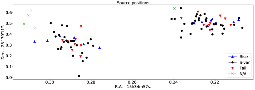
Figure 3: Spatial distribution of all sources given in Tables 3 and 4 with the eastern nucleus to the left and the western nucleus to the right. Each source is coloured by its observational classification (including not classified, or N/A), as described in Sect. 2.5. We note that a few sources are detected in the eastern nucleus outside the central cutout region shown in Fig. 1(a).

In Fig. 3, we show the positions of the sources, coloured by classification. The sources trace a region extended from east to west in the western nucleus, and from south-west to north-east in the eastern nucleus. This is consistent with the orientation of the disks seen at lower spatial resolution at 5 GHz by Barcos-Munoz et al. (2015).

3.1 The luminosity-diameter relation

Fig. 4 shows the 6 cm spectral luminosity versus source diameter for the sources detected in Arp 220, that is the values listed in Tables 3 and 4. The luminosities were calculated from the flux densities measured in BB335B while the sizes were averaged over the BB335 6 cm and 3.6 cm observations as described in Sect. 2.4. In Fig. 4 the data are shown in log-log scale together with 45 SNRs observed in the nearby galaxy M82, using data from Huang et al. (1994). We note that the two brightest SNRs in M82 overlap the weakest objects detected in Arp 220. For discussion purposes, we have also overlayed the evolution of the bright radio supernova SN1986J during its first 30 years, using the 5 GHz flux density measurements presented by Weiler et al. (1990); Bietenholz et al. (2002, 2010) and Bietenholz & Bartel (2017), together with the size evolution after $t$ years of $D[$mas$]=0.86\cdot t^{0.69}$ at distance of 10 Mpc obtained by combining the 1-year radius of 0.43 mas from Bietenholz et al. (2002) with the expansion $\propto t^{0.69}$ from Bietenholz et al. (2010).

The sources with BB336B 6 cm luminosities above $0.5\times 10^{28}$ erg s^-1 Hz^-1 are all consistent with reaching 6 cm peak luminosities of about $10^{28}$ erg s^-1 Hz^-1 during their evolution, see the lightcurves in appendix F. From Fig. 4 we note that most rising sources are relatively small ($D<0.4$ pc). Given their current lightcurves, some of the weaker rising sources are unlikely to reach 6 cm peak luminosities of $\sim 10^{28}$ erg s^-1 Hz^-1, for example 0.2084+0.534, while others for example 0.3011+0.341 may reach these luminosities in a few years time.

The slowly varying sources occupy all regions of Fig. 4. They are all consistent with either being near their 6 cm peak luminosity, or in a state of slow decline. Some of these sources have slowly varying 18 cm lightcurves, for example Fig. 2(c), while others show rapidly changing 18 cm lightcurves, for example Fig. 2(d). Some are optically thin (for example $L_{\text{18\,cm}}>L_{\text{6\,cm}}>L_{\text{3.6\,cm}}$) while others show almost no 18 cm emission while still clearly detected in multiple epochs at shorter wavelengths.

The falling sources also occupy all regions of Fig. 4. Some of these, for example 0.2227+0.482, show relatively rapid (50% in 10 years) optically thick decline from a peak luminosity of $>10^{28}$ erg s^-1 Hz^-1 without any clear 18 cm detection. Others, for example 0.2122+0.482, show an optically thin decline with prominent 18 cm emission since 1994.

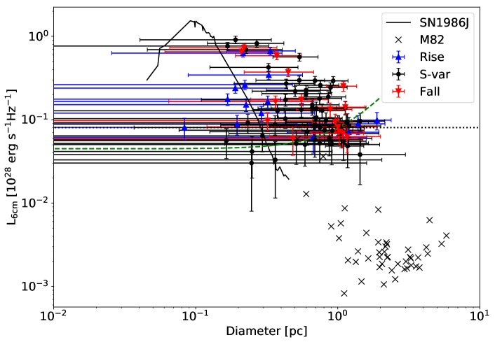
Figure 4: The data in Tables 3 and 4 plotted as spectral luminosity vs diameter in log-log scale. The surface brightness detection limit of BB335B is shown as a dashed line, and the fitted luminosity completeness limit $L_{c}$, as derived in Sect. 3.4, is shown as a dotted line. The lower panel show 45 SNRs in M 82 plotted as black crosses (data from Huang et al. 1994, their Table 2, scaled to 6 cm assuming $\alpha=-0.5$). The evolution of SN1986J during its first 30 years is plotted as a solid curve, from the model described in Sect. 3.1.

3.2 Source expansion from 2008 to 2014?

Given that we have data spanning many years one could try to measure if sources are expanding between the observing epochs. However, an expansion speed of $<10000$ km/s, as expected for the SNe in Arp 220 (Batejat et al., 2011), translates to an increase in diameter of $<0.02$ pc in one year. Even using the most sensitive 6 cm data, such a small increase is very challenging to detect between two single epochs given the uncertainties on our size measurements. Also, older sources are expected to decelerate as well as fade, making any expansion harder to detect.

To reduce uncertainties we average the sizes (as described in Sect. 2.4) for the most sensitive series of 6 cm epochs close in time, that is the epochs within experiments GC031 and BB335, to obtain more robust size measurements separated by about 6 years in time. However, even with these average sizes the uncertainties as too large to probe any expansion. New sensitive high-resolution observations cold possibly help to measure expansion velocities.

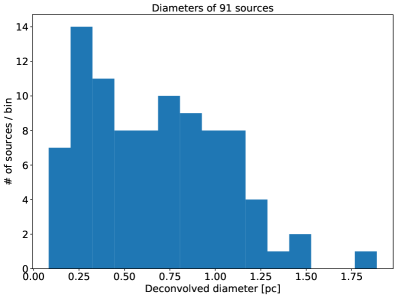
Figure 5: The distribution of measured source diameters appears bi-modal, with peaks around 0.25 pc and 0.8 pc. We note that three of the 97 sources have no size estimates in either BB335A or BB335B and are therefore not included in this figure.

3.3 The measured distribution of source diameters

The measured source sizes are shown as a histogram in Fig. 5, that is a projection of Fig. 4 onto the horizontal axis. The size distribution appears double humped, with peaks around 0.25 pc and 0.8 pc, and falls off around a diameter of 1 pc. We note that the measured sizes have significant uncertainties and stress that Fig. 5 alone is not proof of a bimodal distribution. In general, source sizes may be in error where the actual source structure deviate significantly from our assumed spherical shell model, such as for examplethe case of SN1986J where there is a compact central component present (Bietenholz & Bartel, 2017). The fitted sizes for the smaller sources may also be affected by a Ricean bias, where the fit favours slightly larger sources because negative sizes are not allowed. This effect is tentatively supported by the simulations presented in Table 5, as eight of nine cases with simulated diameter Sim.D $\leq 0.56$ mas were fitted with a larger least-squares diameter. Therefore, the peak around $0.25$ pc may in reality be shifted towards zero. It is hard to estimate how much this would affect the apparent bimodality. If all of the $0.25$ pc sources were in fact point sources, the peak would be shifted but the distribution still bimodal. If, on the other hand, nine sources around 0.3 pc are biased upwards and are in fact unresolved, with no other changes, then the observed distribution would essentially appear uniform. While uncertain, the shape of the distribution is, however, consistent with two underlying distributions truncated by the observational limits in surface brightness. This idea is discussed further in Sect. 4.

3.4 The source luminosity function

The source luminosity function is shown as a histogram in Fig. 6 and as a cumulative function in Fig. 7.

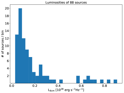
Figure 6: The distribution of measured spectral source luminosities, as measured in the epoch BB335B_C. Nine of the 97 sources were not detected in this epoch, and have therefore been excluded from this figure.

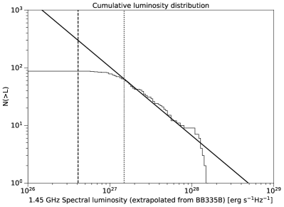
Figure 7: The cumulative luminosity function for the 88 sources detected in BB335B_C (of the total 97 sources detected in all epochs). To be directly comparable with Fig. 1 of Chomiuk & Wilcots 2009, the luminosities have been extrapolated from Tables 3 and 4 to 1.45 GHz, assuming a spectral index of $-0.5$. A power-law fit it shown as a solid line. The point source detection limit is shown as a vertical black dashed line to the left, and fitted completeness limit (where the power law turns over) is shown as a dotted line.

Chomiuk & Wilcots (2009) investigate the SNR LF in 18 ‘normal’ galaxies at 1.45 GHz by fitting the power law

$$n(L)=AL_{24}^{\beta}$$ (5)

where $A$ is a scaling factor (accounting for example SFR), $\beta$ is a negative number (predicted by Chomiuk & Wilcots (2009) to be -2.1) and $L_{24}$ is the 1.45 GHz luminosity given in units of $10^{24}$ erg s^-1 Hz^-1. Using maximum likelihood estimation methods (MLE) Chomiuk & Wilcots (2009) find a slope $\beta=-2.07\pm 0.07$ from combining 258 SNRs in all 18 galaxies, in very good agreement with the predicted value.

In addition to the 18 galaxies, Chomiuk & Wilcots (2009) investigate the LF in Arp 220 using eight SNRs listed by Parra et al. (2007). They find $\beta=-3.00\pm 1.89$ which, although consistent with the predicted value, is uncertain because of the small sample size.

We analyse the Arp 220 LF as sampled by the 88 sources detected at 5 GHz in experiment BB335B. Assuming an average spectral index of $\alpha=-0.5$ (as modelled by Chomiuk & Wilcots (2009) assuming the CR electron energy spectrum can be described as a power law $E^{-2}$), we extrapolate the flux densities measured at 5 GHz (given in Tables 3 and 4) to 1.45 GHz for direct comparison with Chomiuk & Wilcots (2009). We note that this extrapolation likely gives a better estimate of the intrinsic 1.45 GHz emission than directly using values measured at closer frequencies because of the significant free-free absorption affecting the radio emission from Arp 220 below 2 GHz (Smith et al., 1998a; Lonsdale et al., 2006; Varenius et al., 2016). In principle, also the 5 GHz emission may be (slightly) affected by absorption. If so, fitting the luminosity function using 5 GHz data may result in a (slight) underestimate of the intrinsic spectral luminosity function. However, as noted in Sect. 2.5.1, available observations at higher frequencies have lower sensitivity and hence detect fewer sources which we estimate to introduce more significant uncertainties.

To determine $\beta$ in Eq.5 we use the MLE methods of Clauset et al. (2009), that is the same as used by Chomiuk & Wilcots (2009), as implemented in the Python package powerlaw by Alstott et al. (2014). This enables determination of a completeness limit, that is the luminosity where the powerlaw turns over due to for example incomplete sampling of faint sources. The limit is found by creating a power-law starting from each unique value in the data set, then selecting the one that results in the minimal Kolmogorov-Smirnov distance between the data and the fit (see also the Appendix by Chomiuk & Wilcots 2009). We note that this limit is significantly higher than the point source detection threshold, see Fig. 7.

Using the 64 sources above our completeness limit (at 1.45 GHz) of $L_{c}=1.49\cdot 10^{27}$ erg s^-1 Hz^-1 we fit a slope $\beta=-2.19\pm$0.15 for Arp 220, in good agreement with the $-2.1$ predicted by Chomiuk & Wilcots (2009). We note that some sources in our sample (in particular those labelled rising) may not yet have reached the SNR stage. However, these are relatively few and excluding those 14 sources from the fit only changes the slope very marginally well within the given uncertainty (to $\beta=-2.21\pm$0.17).

The observed cumulative luminosity function as well as the best fit of Eq. 5 is shown in Fig. 7 along with the $3\sigma$ point source detection limit (in the BB335B epoch, that is a level similar to the $6\sigma$ limit used in the stacked map) and the fitted completeness limit $L_{c}$. The fact that the completeness limit is significantly above the point source detection limit is not unexpected. Sources at, or below, the limit have resolved sizes so their luminosities are spread over multiple beam areas. Hence, in each beam area they would fall below the point source detection limit. We note that the fitted completeness limit could be a real lower limit to the SNR LF in Arp 220 and not just an observational effect, although this seems unlikely given that the turnover occurs close to where it is expected given that most weak sources are resolved.

By integration of Eq. 5 we obtain an expression for the number of sources above a certain luminosity as

$$N(L>L_{\text{min}})=\int_{L_{\text{min}}}^{\infty}n(L)\,dL=-A\frac{L_{\text{min}}^{\beta+1}}{\beta+1}.$$ (6)

Knowing that $N(L>L_{c})=64$, this expression can be used to estimate a value for $A$. Even though the parameter $\beta$ is assumed to have Gaussian probability distribution (using MLE methods), the distribution of $A$ is clearly asymmetric because of the exponential dependence on $\beta$. We determine $A$ using a Monte-Carlo approach where we sample its distribution using $100,000$ random draws of $\beta$ from a Gaussian distribution with mean $-2.19$ and standard deviation $0.15$. From the resulting distribution of A-values we fit the cumulative distribution function using the interpolation approach implemented in the package SciPy to obtain three empirical quantiles corresponding to the $-1\sigma$, mean, and $+1\sigma$ values for a Gaussian distribution. From this we obtain a robust estimate of $A=461000^{+1068000}_{-325000}$ where the uncertainty reflects the uncertainty in $\beta$. We note that this numeric value of $A$ assumes a luminosity given in units of $10^{24}$ erg s^-1 Hz^-1 in Eq. 5. We also note that if we instead sample $\beta$ from a Gaussian distribution with mean $-2.07$ and standard deviation $0.07$, that is the average value found by Chomiuk & Wilcots (2009), we obtain $A=170000^{+131000}_{-74000}$. Adding the uncertainties in quadrature, we find our estimate to formally differ from the value of $A=57000^{+39000}_{-19000}$ obtained by Chomiuk & Wilcots (2009) for Arp 220. The difference may be due to various factors not explicitly taken into account in the formal uncertainty estimates, such as differences in flux density measurements for the BP129 observations (which provide the spectral index estimates used by Chomiuk & Wilcots (2009) for their Arp 220 sources), as discussed in Appendix E. Finally we note that if we fix $\beta=-2.1$ we obtain $A=218000$.

4 Discussion

As argued by previous studies, for example Parra et al. (2007), we expect a large ($\sim 4$ yr^-1) rate of supernovae in Arp 220, of which only the most radio luminous objects are bright enough to be detected. Detailed studies of the radio emission from these radio luminous SNe in Arp 220 may allow us to constrain the properties of their CSM, and thus for example the mass loss histories of the progenitor stars. However, a detailed discussion of the evolution of each individual object is currently very challenging, given the complexity of SN evolution and the limited time range sampled by the observations at wavelengths shorter than 18 cm, and is therefore deferred to a future paper. In this section we discuss the radio emission following SN explosions, focusing on general properties of the population of compact sources.

4.1 The radio SN/SNR dichotomy

The evolution of the radio emission arising after supernova explosions is often split in a radio SN-stage, where the blast wave is thought to interact primarily with the CSM, and a SNR-stage, where the blast wave interacts with the surrounding ISM. The passage of SN to SNR phase occurs when the supernova blast wave reaches the radius where the pressure of the ISM is approximately equal to the ram pressure of the wind. This is expected to happen earlier for SNe exploding in the high-pressure environments of starbursts than in normal galaxies.

We note that although this dichotomy is useful in many cases, it is an oversimplification of a broad range of possible evolutionary paths, depending on for example the progenitor mass loss history (that is CSM structure), the explosion geometry, the progenitor nature (single/binary), the structure and density of the surrounding ISM, and the magnetic fields in the CSM and ISM (see for example Weiler et al. 2002; Vink 2012; Dubner & Giacani 2015 and references therein). However, as a detailed discussion of the nature of individual objects is planned for a later paper, for the purpose of this discussion we adopt these simple labels of SNe for objects interacting primarily with their CSM, and SNRs for objects interacting primarily with the surrounding ISM.

4.2 Radio emission from SNe and SNRs

The intensity of radio emission from core-collapse SNe versus time is closely related to the density profile versus radius in the CSM. This relationship is complicated because of the presence of HII-regions and wind-blown bubbles which may have formed around the progenitor stars before the explosion. The structure of the CSM may be complex with for example layers having different densities and temperatures depending on the wind history of the progenitor (for example Weiler et al. (2002); Vink (2012)).

Core-collapse SNe may show prominent emission within a few days after the explosion (for example SN1993J; see Martí-Vidal et al. 2011 and references theirin). In other cases it can take years for the radio emission to appear.

The observed radio emission is thought to come from a region right behind the SN blast wave, where charged particles are accelerated to relativistic energies and trapped in strong magnetic fields (Weiler et al., 2002). If the SN explodes in a low density CSM, very little radio emission is expected until the blast wave reaches the surrounding ISM. If, on the other hand, the SN explodes in a relatively high density CSM, the SN is expected to show a characteristic radio lightcurve, with the peak appearing later at longer wavelengths due to the free-free absorption by the ionised CSM (Weiler et al., 2002).

In a simple model, the radio emission is expected to increase (again) when the shock reaches the dense ISM (i.e the SNR phase) and particle acceleration becomes efficient. The maximum luminosity during this phase is expected to occur at the Sedov radius, where the mass swept up by the blast wave is equal to the mass of the SN ejecta and the energy in relativistic electron reaches a maximum.

In the case of a very dense progenitor wind, that is a dense CSM, it is possible that the Sedov radius is reached already before the shock enters the ISM. For such objects there may not be a clear observational distinction between the SNe and SNR phases. Progenitors with such dense winds are however expected to be rare, and the majority of SNe explosions in Arp 220 will likely produce weak and undetectable radio emission in the initial CSM phase and the sources will rise to a peak radio emission only when they begin interacting with the ISM.

4.3 The nature of the compact objects in Arp 220

Although most radio SNe may be relatively weak and hence below our detection limit, some may brighten enough to be detected when they reach the ISM. In addition to these SNRs (that is shocks interacting with the ISM), we expect to see the most radio luminous SNe which interact strongly with their dense CSM. According to Fig. 1 by (Chevalier et al., 2006), the most radio luminous SNe are of types 1b/c or IIn. Type 1/bc SNe have a relatively short rise time before they start to decline. Since the data presented in this paper sample the evolution sparsely in time, for example every few years or months, we are unlikely to see type Ib/c SNe near these high peak luminosities. However, SNe of type IIn also reach very high luminosities and appear to have significantly longer rise times (few years). These would be seen in our observations, and should be present with similar luminosities in adjacent observing epochs with similar frequency. While type IIn SNe may be a likely explanation for bright sources in our data, these particular type of SNe are, however, thought to be rare and likely make up only a few percent of the total SN population (Smith et al., 2011; Eldridge et al., 2013). It is therefore of interest to study the population of the brightest sources in our data, and to estimate the rate of these luminous events in Arp 220.

4.3.1 The nature of the brightest objects

The brightest objects in Fig. 4 all show lightcurves (see Appendix F) consistent with expansion in a dense, ionised CSM. Indeed, given expansion velocities of a few thousand km/s and high luminosities, multiple objects have significantly longer rise times than expected if synchrotron self-absorption is the dominant absorption mechanism (see Fig. 2 of Chevalier et al. 2006). It is thus likely that free-free absorption from the ionised CSM is significant in these objects.

Given the background presented in Sect. 4.2 we expect to see a few objects in the early radio SN-stage, rising at 3.6 and 6 cm but with weak or undetected 18 cm emission, such as 0.2262+0.512 (see Fig. 2(a)). Objects with high explosion energies evolving in a dense, ionised CSM are then expected to reach their respective peak luminosities later at longer wavelengths, such as 0.2195+0.492 (see Fig. 2(c)), followed by an optically thin decline such as 0.2122+0.482 (see Fig. 2(f)). As the shock wave reaches the ISM, the lightcurves may, in case of a sharp boundary to a higher-density ISM, rise at all frequencies, such as 0.2108+0.512 (see Fig. 2(b)) or, in case of no sharp boundary, flatten (as seems to be the case for 0.2122+0.482 in 2014) due to the constant density. The subsequent SNR phase, when the blast wave expands in the constant density ISM, is expected to show a slow optically thin decline, such as observed in 0.2171+0.484 (see Fig. 2(d)). Because multiple studies (for example Smith et al. 1998a; Lonsdale et al. 2006; Varenius et al. 2016) argue that (foreground) free-free absorption may significantly reduce the measured 18 cm flux densities, we expect to see a few sources, in particular towards the centres of the nuclei, with relatively weak 18 cm emission. This could explain the spectrum of 0.2122+0.482. Also 0.2253+0.483 (see Fig. 2(e)) could be an example of a blast wave hidden behind significant foreground absorption.

4.3.2 Modelling the lightcurves of the brightest object

It is challenging to derive accurate age estimates from the observed lightcurves, mainly because of the limited time coverage at 5 GHz and higher frequencies. Based on the lightcurves the brightest sources are, in general, likely a few decades old with 6 cm rise times of a few years. One way to estimate the age of the brightest sources is to use model-fitting of the lightcurve for an example object. As an example, we choose the brightest object 0.2195+0.492, given that this object has the highest signal-to-noise and therefore should be the first candidate for model fitting from a data quality point of view. We used a simplified version of the model presented by Weiler et al. (2002), as described by Eqns. 1 and 2 of Marchili et al. (2010). This model follows the one presented by Chevalier (1982a, b) where the radial density profile of the CSM is assumed to be $\propto r^{-2}$, The best-fit parameters are $\alpha=-0.93$, K₁=319 Jy, K${}_{2}=4.0\times 10^{9}$, $\beta=-1.33$, and an explosion date of 1981-05-23 that is an observed age estimate (in BB335) of about 33 years, and a corresponding 6 cm peak time of about 17 years. This is significantly longer than the 1210 days listed as the longest rise-time in Weiler et al. (2002) (for SN1986J). The model is shown together with the data in Fig. 8. The fitted values imply a deceleration parameter $m=0.87$ (from Eq. 7 by Weiler et al. 2002) and a pre-supernova mass-loss rate of $3.9\times 10^{-4}$ M_⊙yr^-1, assuming a pre-supernova wind speed of 10 km/s for a type II SN (Weiler et al. 2002; Eq. 18). We note that the estimated mass-loss rate is similar to known type II SNe such as SN1988Z as presented in Table 3 by Weiler et al. (2002). Given the age (and relatively modest deceleration) obtained and the measured diameter of 0.2195+0.492 of about 0.2 pc, a linear estimate implies an expansion velocity of $\sim 3500$ km/s, that is consistent with the few thousand km/s expected for these objects.

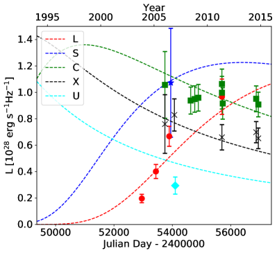
Figure 8: The best-fit lightcurve model described in Sec. 4.3.2 overplotted on the observed detections of 0.2195+0.492. L on the vertical axis denotes spectral luminosity. The S-band data point has been displaced 200 days to the right to make it clearly visible in this plot.

4.3.3 The observed number of luminous SNe

In Sect. 4.3.2 the brightest object is estimated to be about 30 years old. The lightcurves of other objects with similar current luminosity and size indicate a similar evolutionary history. If we, to increase sample size, select as luminous SNe the nine objects with L${}_{\mathrm{6\,cm}}>0.5\times 10^{28}$ erg s^-1 Hz^-1 and diameter $<0.4$ pc, and assume these are at most 50 years old, this would correspond to an observed rate of the most luminous SNe of $\sim 0.2$ yr^-1.

Given the total star formation rate of Arp 220 of 230 M_⊙yr^-1 (Varenius et al., 2016) and using Eq. 2 in Smith et al. (1998b), assuming the same $m_{l}=1\text{M}_{\odot}$, $m_{u}=45\text{M}_{\odot}$ and $m_{\text{sn}}=8\text{M}_{\odot}$, we estimate a total SN-rate of about 4 yr^-1. If 5.6% (average of Smith et al. (2011); Eldridge et al. (2013)) of these end up as type IIn during 50 years of continuous star formation, we expect to see 10 such objects, or a rate of luminous SNe of $0.2$ yr^-1, that is in excellent agreement with the observed number. This suggests that a standard IMF in Arp 220 can explain the number of bright SNe observed in Arp 220. However, this assumes not only that all the brightest SNe are type IIns, but also that all type IIn SNe in Arp 220 reach these high luminosities.

If some IIn peak below our detection threshold, our measured rate would be too low. Furthermore, even though unlikely given the sparse sampling in time, we may still detect some very rapidly evolving SN of types Ib/c and misinterpret these as a IIn. If this is the case, our measured rate could be too high. We stress that both the measured and expected values likely suffer from small sample numbers, where for example a few of the small rising sources may rise above $5\times 10^{28}$ erg s^-1 Hz^-1 within a few years. Finally, our SN-rate estimate are subject to uncertainties related to for example the age estimates of the observed source population.

A more thorough analysis of the data to constrain the IMF in Arp 220 should therefore include careful, detailed modeling of multiple compact sources to better constrain for example source ages. This is however beyond the scope of this work, and will be the subject of a future paper. In addition to the data presented here, this future work will include new global VLBI observations. These data will help to further constrain the evolution of these objects and hence the rate of very luminous SNe in Arp 220.

4.3.4 The nature of the weaker objects

The majority of objects in Fig. 4 have luminosities below $5\times 10^{27}$ erg s^-1 Hz^-1, and these sources are also (based on visual inspection of the lightcurves in appendix F) unlikely to have reached much higher luminosities during their evolution. The position of this population in Fig. 4 is consistent with these being smaller diameter versions of the ISM interacting SNRs in M82. Lacki & Beck (2013) argue that particles accelerated in the SNe in such environments as the nuclei of Arp 220 would have a maximum radiative lifetime of about a thousand years (see their Fig. 1). These calculations assume the electrons are embedded in an ISM magnetic field of 2 mG in Arp 220. In fact, fields in the SNR shells may be a factor of 10 larger (Batejat et al., 2011) and hence lifetimes shorter, but in this paper we assume a conservative figure of 1000 yrs. Given the SN-rate of 4 year^-1, we would hence expect at most 4000 radiating SNe/SNRs present in the galaxy. The fact that we observe only $\sim 2.5\%$ of that number could be explained by a majority of the SNRs having significantly shorter lifetimes. However, given that many sources detected in this work are close to our detection limit, there may very well be a significant number of weaker sources present but not yet detected.

Berezhko & Völk (2004) show that less energetic SNRs expanding in lower densities reach lower peak luminosities at larger sizes (see their Fig. 4). This means such SNRs may only peak when larger than 0.5 pc and be missed by our surface brightness limited observations. In addition, the dependence of peak radio luminosity on explosion energy $E_{\text{sn}}$ is very strong: in the Sedov phase the luminosity is expected to scale with $E_{\text{sn}}^{7/4}$, that is a factor of four less energy implies 10 times weaker peak luminosity. Since many sources are observed just above our detection limit, it is reasonable to assume that these are the brightest objects of the radiating population.

We conclude that the fainter objects may very well be the tip of a distribution of supernova remnants, where the majority have luminosities below our detection limit. Indeed, the brightest of these fainter objects sources, with diameter $>0.4$ pc but $L_{\mathrm{6\,cm}}<3\cdot 10^{28}$ erg s^-1Hz^-1 (see Fig. 4), for example 0.2171+0.484, 0.2211+0.398, and 0.2360+0.431 are all consistent with being observed close to their 6 cm peak (see for example panel d in Fig. 2 and appendix F). Furthermore, these three sources are all long lived with stable lightcurves, suggesting they are more likely in the more-slowly-evolving SNR phase, rather than in SN phase like the most luminous sources discussed above. Also, these sources show prominent 18 cm emission, indicating the blast wave has reached outside the ionised CSM.

4.4 The distribution of source sizes

We argue above that some small ($D<0.4$ pc) and luminous $L_{\mathrm{6\,cm}}>5\cdot 10^{28}$ erg s^-1Hz^-1 objects are examples of the relatively rare radio luminous SNe, which interact strongly with a dense and ionised CSM. We also argue that the larger (and weaker) sources are SNRs, that is where the SN blast wave is interacting with the dense ISM. Two source populations are also consistent with the tentative bimodal size distribution, see Fig. 5. We stress, however, that most size estimates have significant uncertainties.

4.5 Is the smooth GHz-emission of Arp 220 a collection of compact objects?

Barcos-Munoz et al. (2015) image Arp 220 at 4.7 GHz with lower angular resolution and measure a total flux density of 222 mJy. Their measurement includes both the emission from compact objects, detected in VLBI observations, as well as smooth emission on scales resolved out by the VLBI observations presented in this paper. The total flux density measured in the 88 continuum sources from Tables 3 and 4 is 22.5 mJy, that is 10% of the total flux density measured by Barcos-Munoz et al. (2015). The fitted completeness level of the observed luminosity function in Sect. 3.4 and the detection limit shown in Fig. 4 strongly suggests that there are many more radiating sources in Arp 220 than we observe in this work. Could the sources below our VLBI surface brightness detection limit be the source of the smooth synchrotron emission detected by for example Barcos-Munoz et al. (2015)?

As a simple empirical estimate of the relative contribution of compact sources to the integrated flux density, we take the observed luminosity function and extrapolate this to luminosities below our detection threshold. If we assume all SNe give rise to an SNR, and an upper radiative lifetime of 1000 years, we expect, given the above SN-rate of about 4 yr^-1, at most 4000 objects in Arp 220, of which we observe the brightest $\sim 2$ percent. Given a total number of 4000 SNRs, we can use Eq.6 to obtain a distribution of $L_{\text{min}}=4.6_{-1.8}^{+2.2}\times 10^{25}$ erg s^-1 Hz^-1 (at 1.45 GHz) given a distribution of $\beta$. The distribution of $A$ is determined from Eq. 6 assuming 64 sources brighter than our completeness limit as described above.

If we integrate $n(L)L$ from $L_{\text{min}}$ to the observed $L_{\text{max}}\approx 2\times 10^{28}$ (at 1.45 GHz) we obtain the distribution of the total luminosity from compact sources as

$$L_{\text{tot}}=\int_{L_{\text{min}}}^{L_{\text{max}}}AL^{\beta+1}\,dL=\cases{}{A}{\beta+2}\left(L_{\text{max}}^{\beta+2}-L_{\text{min}}^{\beta+2}\right),&\text{if $\beta\neq-2$}.\\ A\ln(L_{\text{max}}/L_{\text{min}}),\text{if $\beta=-2$}.{}$$ (7)

Using 100,000 random draws of $\beta$ (with mean $-2.19$ and $\sigma=0.15$) we sample the distribution of $L_{\text{tot}}$ to estimate uncertainties. In this calculation, the parameter A is again a distribution determined from Eq. 6 assuming 64 sources brighter than our completeness limit as described above. Assuming $\alpha=-0.5$ we obtain a total 5 GHz flux density from 4000 compact sources of $L_{\text{tot}}=56^{+9}_{-8}$ mJy. As done above, the uncertainties correspond to $\pm 1\sigma$ for a Gaussian distribution, calculated using fitting to the sampled cumulative distribution function. Given that 4000 radiating sources is an upper limit, it follows that a source population described by the powerlaw distribution in luminosity defined by Eq. 5 can account for at most 25% of the total flux density observed from Arp 220 at GHz frequencies. So what is the source of the remaining radio emission measured by Barcos-Munoz et al. (2015)?

The above argument assumes a maximum lifetime of CRs in the SN shocks of a thousand years. While the actual lifetime of accelerated CRs is likely shorter given the strong magnetic fields in the shocked regions (as noted in Sect. 4.3.4), the dense ISM in Arp 220 means that the SNR shocks will encounter significant particle densities also after leaving the CSM. Although each accelerated CR cools relatively quickly, the blast wave may posses significant kinetic energy for hundreds of years. During this time, particles in the ISM may be (re-)accelerated to emitting energies, long after the initial CRs accelerated in the ISM when entering the Sedov phase have faded. In addition, the massive progenitor stars likely form in dense star clusters of sizes of a few parsec (Wilson et al., 2006). In this case, SN shock waves with diameters larger than 1 pc (which may be too faint to be detected in Fig. 4) may collide with each other. The combined mechanical energy may be enough to compress the ISM to even higher densities and accelerate CRs to cause significant radio emission (Bykov, 2014). In addition, given the high densities in Arp 220, also protons accelerated in the SN shocks may cause significant synchrotron radiation via collisions with ISM which produce secondary electrons and positrons, thereby more efficiently radiating the energy in the SN shocks (Lacki et al., 2010). This would imply that the fitted luminosity function has a significant tail of a large number of weak sources, compared to when extrapolated from the powerlaw in Fig. 7. This could potentially explain the origin of the smooth radio emission.

Another explanation could be an AGN contribution to the radio emission. However, a significant AGN contribution would likely manifest itself in a radio-bright compact core, and/or radio jets. While we do not find any clear support in terms of for example radio jets to support a recent significant AGN contribution to the radio emission, it is still possible that an AGN could play an important role in this galaxy, since its activity could be episodic and any jet like structure dissolved into smoother structure by merger forces, and the emitting structure thereby hidden from VLBI observations due to lack of spatial scales sampled.

Future observations with very high sensitivity, possibly combined with stacking of the current available data as well as tapering and statistical analyses of possible non-Gaussian contributions to the image noise, may reach sufficient sensitivities to detect or exclude such a population of weak sources, and/or further constrain any AGN contribution.

5 Summary and outlook

In this paper we have presented data from 20 years of VLBI monitoring of Arp 220. We detect radio continuum emission from 97 compact sources, and find they follow a luminosity function $n(L)\propto L^{\beta}$ with $\beta=-2.19\pm 0.15$, similar to SNRs in normal galaxies. The spatial distribution of sources trace the star forming disks of the two nuclei seen at lower resolution.

We find evidence for a Luminosity-Diameter relation within Arp 220, where larger sources are less luminous. The exact form of the relation is however hard to quantify because of a range of selection effects. The observed distributions of source luminosities and sizes are consistent with two underlying populations. One group consists of very radio luminous SNe where the emitting blast wave is still inside the dense, ionised CSM. The other group consists of less luminous and larger sources which are thought to be SNRs interacting with the surrounding ISM.

Assuming all SNE type IIn reach the highest luminosities, and assuming the brightest sources we detect are IIns, we find that the observed number of very luminous SNe is consistent with expectations given a standard initial mass function and the total integrated star formation rate of the galaxy. This result should however be taken with care, as more detailed modeling of multiple sources is needed to better constrain the evolution, and in particular the ages, of the most luminous SNe.

When extrapolating the observed luminosity function below our detection threshold we find that the population make up at most 20% of the total radio emission from Arp 220 at GHz frequencies. However, secondary CR produced when protons accelerated in the SNRs interact with the dense ISM and/or re-acceleration of cooled CRs by overlapping SNR shocks may increase radio emission from the sources below our detection threshold, compared to the extrapolated value. This mechanism may provide enough emission to explain the remaining fraction of the total radio flux density, and could potentially be constrained by future high-sensitivity observations.

Continued high-sensitivity VLBI monitoring of Arp 220 will likely detect many more fainter sources and therefore probe the distribution of lower luminosities and larger sizes which may further constrain the evolution of SN/SNRs in extreme environments. Results from similar ongoing monitoring of other galaxies, such as the closer LIRG Arp 299 (Perez-Torres et al. in prep.) will be interesting for comparison to the results presented in this work.

Appendix A Data and scripts in the CDS

Data, images and analysis scripts presented in this paper are available in electronic form at the CDS via anonymous ftp to cdsarc.u-strasbg.fr (130.79.128.5) or via http://cdsweb.u-strasbg.fr/cgi-bin/qcat?J/A+A/. The material is split in five directories. The calibration directory contains one subdirectory per experiment. Each subdirectory contains a ParselTongue script, and in some cases also some additional files, used to calibrate archival UVFITS data to obtain FITS images. The fitsimages directory contains the FITS images obtained for all observations analysed in the paper. There are two images for each experiment, one for each nuclei in Arp 220. The stacking directory contains the stacked images obtained by stacking together all images at each band, as well as the script used to perform the stacking. The stacked 6 cm images are also displayed in Fig. 1. The fitting directory contains the Python scripts used to fit spherical shell models to sources in the FITS images for all epochs. The output of the fitting is stored in the directory fitresults as ASCII files. These contain the fitted values for position, flux density and diameter for all sources in all experiments.

Appendix B Calibration and imaging

B.1 Phase calibration and positional uncertainty

For most epochs phase calibration started by removing bulk residual delays and rates, using one of the three bright sources J1516+1932 (ICRF J151656.7+193212), J1613+3412 (ICRF J161341.0+341247) or OQ208 (ICRF J140700.3+282714) by running the AIPS task FRING. This should also remove relative phase differences between the spectral windows (AIPS IFs). However, multiple epochs showed time variable phase differences between the IFs. This was corrected for by running FRING also on the phase-reference source J1532+2344 (ICRF J153246.3+234405) for epochs where this source was included in the observations.

Experiments BP129, GC028, GC031, BB297 and BB335 were all phase-referenced to the nearby (0.55^∘) compact calibrator J1532+2344, assumed to be located at R.A. $15^{h}32^{m}46^{s}.3452$, Dec. $23^{\circ}44^{\prime}05^{\prime\prime}.268$, and Arp 220 was correlated at position R.A. $15^{h}34^{m}57^{s}.250$, Dec. $23^{\circ}30^{\prime}11^{\prime\prime}.33$, that is between the two nuclei. After transferring the phase-reference corrections, an initial image was made of Arp 220. In many cases, the resulting image showed beam like artefacts around bright sources consistent with residual phase errors. To remove the residual phase-errors, phase self-calibration (see for example Cornwell & Wilkinson 1981) was used with the initial phase-referenced image as calibration model.

The self-calibration step removed obvious phase-errors, and generally improved the images. However, because Arp 220 is weak at mas-scales (5-35 mJy in these data), a low baseline SNR threshold of 2 was required. Such a low threshold may introduce spurious sources or in other ways impact the data in a negative way (Martí-Vidal & Marcaide 2008). To assure the validity of the self-calibrated results, we checked

1. The general image quality: Did the self-calibration cycle remove obvious phase-errors, such as convolution like artefacts on all sources?

2. The RMS noise in central regions with many sources: Did it decrease after self-calibration?

3. The source flux densities: Did the source flux densities increase as expected after self-calibration?

4. The phase-solutions: Although noisy, were the solutions tracing slowly varying atmospheric errors and/or clear antenna offsets?

5. The consistency with all available data: Were the flux densities and sizes, measured for a particular epoch, consistent with the information from all other epochs?

In summary, we found clear signs of improvements in image quality for most epochs, and no clear sign of corruption due to self-calibration. We note that we only performed one cycle of self-calibration, which leaves little room for spurious sources to grow bright, as can sometimes happen after many cycles of poorly constrained self-calibration. We note that only phase-corrections, that is no amplitude corrections, were derived using self-calibration of Arp 220.

In contrast to the phase-referencing above, four 18 cm experiments, GL021, GL026, GD017, and GD021, were phase-referenced to compact OH-maser emission within Arp 220 itself. Phase corrections were derived from self-calibration using the strongest maser channel. Initially, a point source model was used, but in all cases the elongated structure of W1 (see Fig. 1a of Lonsdale et al. (1998)) was recovered after a single iteration. One or two additional self-calibration iterations were carried out to ensure the structure of the maser was correctly taken into account. The corrections derived for this single channel were then applied to all channels of all spectral windows. No further self-calibration of Arp 220 was performed for these epochs. Note that no high-resolution spectral data were used (although in some cases available in the archive). Instead, we used a single broad frequency channel in the continuum data, containing the maser emission, to obtain corrections for residual phase errors.

The three 18 cm experiments GL021, GL026, and GD017 used a correlation position of R.A. 15^h34^m57^s.2247, Dec. 23^∘30^′11^′′.564 for Arp 220, while GD021 used the same as BP129. By phase self-calibration of the brightest maser channel (in the continuum data), the position of all compact sources were anchored to the peak of the compact maser. In this work, we assume a peak position of the maser W1 of R.A. $15^{h}34^{m}57^{s}.22435$, Dec. $23^{\circ}30^{\prime}11^{\prime\prime}.6644$. This position was obtained from imaging the maser emission in the phase-referenced 18 cm data taken in experiment BB297A. Since BB297A was phase-referenced to J1532+2344 (and did not use the maser for phase calibration), we thereby align the maser calibrated epochs to the common reference position of J1532+2344 used for the other epochs. We assume that the maser position does not vary between the observations. Cross-correlation of the resulting continuum images among the different epochs supports this assumption.

Given that many sources are close to our surface brightness detection limit, and the fact that many are resolved which may impact the peak position, we assume a conservative uncertainty of 1 mas for all source positions within Arp 220. Notes on position offsets for particular sources can be found in Appendix E.2.

B.2 Amplitude calibration

The amplitude calibration of all epochs was anchored to the measurements of system temperatures and gains of VLBA antennas. The procedure applied to ensure the best possible amplitude calibration was as follows:

1. Apply á priori amplitude calibration to all antennas, using measured system temperatures and antenna gain curves.

2. Determine a set of good, self-consistent, antennas (usually the VLBA), excluding antennas with obvious amplitude offsets seen in amp vs. UV-distance plots.

3. Perform amplitude self-calibration of the good antennas to correct minor errors, using imaging of a bright observed source, that is J1516+1932, J1613+3412 or OQ208, depending on data set.

4. Amplitude self-calibration of previously excluded antennas, fixing the good antennas, using the same bright source. We note that if sensitive antennas with a major error are included from the start, the whole flux scale may be shifted due to their large weight.

5. Either, for phase-referenced epochs: derive amplitude corrections for the target by imaging and (self-)calibrating the phase-reference source, or,

6. For some maser-calibrated epochs: derive amplitude corrections for the target by imaging and (self)-calibrating the maser emission.

7. Apply cumulative antenna based corrections to the Arp 220 observations.

We adopt an absolute flux calibration uncertainty of 10% for all data.

We note that the noise we obtained in some re-reduced observations is larger than in some previous publications (for example Lonsdale et al. 2006). This may be explained by several factors. First, multiple non-VLBA antennas had to be excluded from our processing, since no system temperatures or gain measurements could be found (these seem to have been lost as they are not available via for example the NRAO or JIVE online archives). Second, because of the large amount of data processed in this work and our efforts to use a similar calibration and imaging strategy for all data, we may have missed opportunities to improve specific epochs by for example elaborate weighting of very sensitive antennas, or extra careful editing of bad data.

For the 6 cm data sets GC031B and GC031C, a careful analysis of the final images, made after using the calibration strategy outlined above, revealed both these epochs to be systematically too bright for all sources, although their relative flux densities were reasonable. These offsets were also found when comparing the amplitudes of the uncalibrated visibilities on multiple VLBA baselines to the corresponding baselines in BP126 and BB297A. We also found consistent offsets in the recovered flux densities of the bright calibrator J1516+1932 in these epochs. We believe that these epochs were affected by an error, scaling the visibilities to higher values before storing them in the archive. Further investigations of this error is however beyond the scope of this work. For the purpose of this work, we derive a scaling factor for each of the two epochs, based on a requirement of continuity for the light-curves of the brightest sources, as well as the observed differences in the raw uncalibrated visibilities. The correction factor derived for both epochs was 0.70, and it was applied to the images before any analysis of these epochs.

B.3 Bandpass calibration

For all epochs, bandpass corrections were derived using a bright observed source, that is J1516+1932, J1613+3412 or OQ208, depending on data set, assuming these sources to have a flat spectrum across the observing bandwidth.

B.4 Imaging

All epochs were imaged using the CLEAN deconvolution algorithm as implemented in the task IMAGR in AIPS, using two fields to simultaneously clean the two nuclei. All epochs were imaged in a two-step auto-boxing procedure, as implemented in IMAGR. First, boxes were automatically placed by IMAGR on the brightest sources, defined as having peak signal-to-noise ¿ 10 and source island level ¿ 5. This minimised the risk of cleaning strong side lobes caused by the synthesised beam. Then, the boxes were removed and a few hundred clean iterations ran without any box-restrictions to find weaker sources. The imaging was stopped when the CLEAN algorithm converged, that is when no significant amount of flux was recovered in a few hundred iterations. The final images were exported to FITS for further analysis outside AIPS. The number of pixels used were 8192 in R.A. and Dec. for all images. For the 2 cm data, a pixel size of 0.05 mas was used. All other epochs used a pixel size of 0.1 mas. Robust weighting (Briggs 1995) of 0.5 was used for all images.

Appendix C Model fitting

In this work we fit models of sources to CLEAN images. In principle, it is best to fit models directly to the calibrated visibilities to avoid any effects introduced by the deconvolution (for exampleMartí-Vidal et al. 2014). However, visibility fitting of multiple nearby sources involve simultaneous fitting of all parameters for all sources. Because of the large number of sources in Arp 220, and the large number of datasets analysed in this work, simultaneous visibility fitting is not feasable. We therefore decided to fit models to the CLEAN images, which allows us to work on a small subimage encompassing each source. We decided to use least-squares (LS) optimisation to find the optimal model for each source. We verified the validity of this approach by comparing it with visibility fitting of simulated data, see appendix D.1. Below we describe in detail how the fitting was done for each source. We note that the Python code used to do the fitting is available via the CDS as described in A.

C.1 Preparing a stamp image

First a small subimage, hereafter called a stamp, was extracted from the cleaned image, centred on the source catalogue position in Tables 3 and 4. The stamp was selected as $128\times 128$ pixels at bands C and X, and $256\times 256$ pixels at bands L, S and U. The number of pixels are chosen to fully cover the source being fitted, and any nearby sources, with enough source-free pixels around to avoid edge-effects, and then rounded upwards to the next power of 2 to enable FFT optimizations. A threshold was imposed to only fit stamps with clear emission present in the centre. If the central $2\times 2$ mas did not contain a peak value of at least three times the experiment RMS noise (see Table 1), no fit was attempted.

C.2 Defining the model

We assume each stamp to be an estimate of the true source convolved with a beam and sampled on a discrete grid of pixels. Each source is assumed to be a projection of an optically thin spherically symmetric shell with 30% fractional shell width. The convolving beam was taken to be the Gaussian CLEAN restoring beam for each stamp. We chose to discretise the expressions for shells and beams in Fourier space, replacing the computationally intensive convolution with a multiplication. In other words, in each fitting-iteration, we define and discretise our shell and beam in Fourier-space. The convolved shell-model, constructed in Fourier space, is then transform to an image for calculation of LS residuals, that is comparison with the CLEAN stamp. We stress that this approach gives results with similar accuracy to visibility fitting on simulated data, see Appendix D.

C.2.1 Constructing a shell

We construct a model of a shell by subtraction of two spheres. The spheres are defined in Fourier space using the analytical expression of a projected sphere of unit flux density, that is Eq. 16-28 of Pearson (1999):

$$\mathcal{F}(f(x,y,d))=\frac{3}{(\pi d\rho)^{3}}\left[\sin(\pi d\rho)-\pi d\rho\cos(\pi d\rho)\right]$$ (8)

where $d$ is the sphere diameter, $\rho=\sqrt{u^{2}+v^{2}}$ and $u,v$ are the spatial frequencies along the $x,y$ directions respectively.

A thin shell $f_{s}$ with flux density $I$ is formed as the difference of two spheres with 30% fractional width, scaled in flux density by their respective volumes, as

$$f_{s}(x,y,d,I)=I\frac{4\pi}{3}\frac{\left(f(x,y,d)\cdot d^{3}-f(x,y,0.7d)\cdot(0.7d)^{3}\right)}{(4\pi d^{3}/3-4\pi(0.7d)^{3}/3)}$$ (9)

where $I$ is the integrated flux density of the shell with outer diameter $d$ and inner diameter $0.7d$. This expression is deliberately not maximally simplified, to better illustrate the constituents. For computational efficiency, we discretise also the Gaussian beam directly in Fourier space. This allows us to calculate the elementwise product of the Fourier transforms of the shell and beam. We then used an inverse Fast Fourier transform (IFFT), as implemented in the python module numpy.fft.ifft2, to obtain the pixelated convolved shell $m_{i,j}$ in the image domain for comparison with the stamp. According to the well known convolution theorem, this is equivalent to convolution in the image domain, that is $m(x,y,d,I)=\mathcal{F}^{-1}(F\cdot H)$ where $m$ denote the concolved shell in the image domain, and $F$ and $H$ denote the shell and beam in Fourier space.

The residual vector used by the LS minimisation routine was calculated by forming the weighted pixelwise difference as

$$\mathrm{res}_{ij}=\frac{(m_{ij}-d_{ij})^{2}}{E_{f_{ij}}^{2}}$$ (10)

where $m_{ij}$ is the convolved model and $d_{ij}$ is the image data. $E_{f}$ is defined in Eq. 1 with subscripts $ij$ referring to the flux density in pixel number $i$ in R.A. and $j$ in Dec. The residual was minimised using the Python library scipy.optimize.least_squares which enables bounded LS fitting. The minimisation was allowed to simultaneously vary the flux density, size, and position of the shell. The flux density was required to be $>0$, the size $\leq 8$ mas, and the position in R.A. and Dec. was restricted to be within $\pm 1$ mas of the stacked catalogue position listed in Tables 3 and 4. The initial guess was the same for all fits: flux density 0.5 mJy, size 0.1 mas (1 pixel), and position as in Tables 3 and 4.

Most sources were very well centred, but a few clearly resolved shells had minor offsets since the PyBDSM algorithm had found the peak at one side of the shell. An example of this can be seen in Fig. 9. When the fit converged, the best-fit model was transformed to the image plane and subtracted from the working-copy of the cleaned image to simplify fitting of other nearby sources. The best-fit parameters were saved to disk and values for all attempted fits are available as electronic tables through the CDS as described in A.

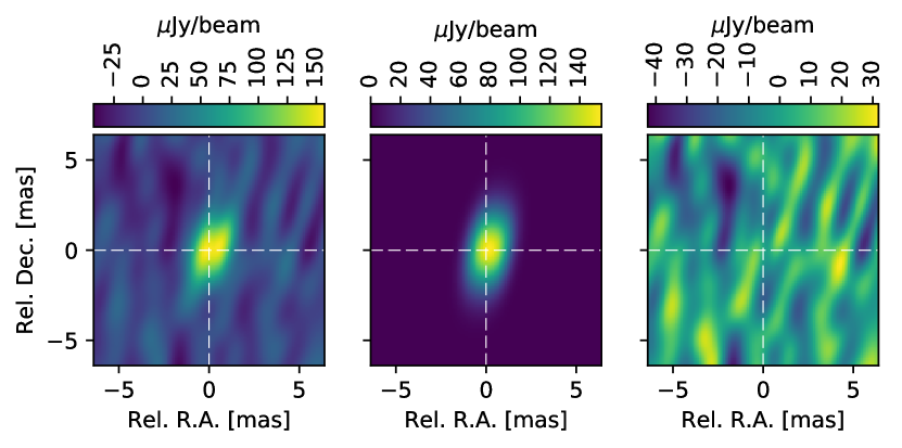
Figure 9: Example fitting of a clearly resolved source 0.2212+0.444 in the 6 cm image of BB335B. The left panel shows the CLEANED image (the observation), the mid panel the best fit model convolved with the CLEAN beam, and the right panel the residual that is image$-$model. The white cross marks the centre of each panel, that is the position guess obtained from PyBDSM. This particular fit was chosen because it shows that the position found by PyBDSM may be off when PyBDSM’s Gaussian fitting finds the peak of one of the two beam-features of a weak resolved shell. However, since the position is allowed to vary, this taken into account in the fitting, as seen here where the fitted position is a little to the right of the white cross.

C.3 A self-consistent check of the catalogue positions

The source positions in Tables 3 and 4 were obtained by PyBDSM as described in Sect. C. However, one may ask, do the stacked images really provide a good reference for the catalogue, or for initial guesses for the fitting routine? To check this we compiled two figures of the difference between the catalogue R.A. and Dec. and the fitted R.A. and Dec for all modelfits done in this work, see Fig. 10.

The majority of fitting results are well within our target accuracy of $\pm$1 mas. Note that 18 cm fits are not included in this figure; the spread in R.A. is very similar for 18 cm, but the fitting in Dec. is much less well constrained because of the relatively large major axis of the synthesised beam which in most epochs extends towards north-south.

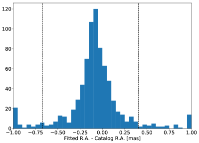
(a) Right Ascension

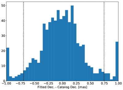
(b) Declination

Figure 10: Comparison of fitted positions with catalogue positions given in Tables 3 and 4. The dashed lines mark the 5% and 95% percentiles. The majority of fitting results are well within our target accuracy of $\pm$1 mas. The larger dispersion in Dec. compared to R.A. is explained by the synthesised beam being elongated approximately north-south in most epochs. Note that 18 cm fits are not included in this figure; the spread in R.A. is very similar for 18 cm, but the fitting in Dec. is much less well constrained because of the relatively large major axis of the synthesised beam.

Appendix D Comparison of fitting methods

In this work we have used LS optimisation to fit source flux densities and sizes to deconvolved images. LS-fitting is widely used and is very quick. It is, however, challenging to obtain meaningful uncertainty estimates from the fitting procedure itself (see for example Hogg et al. (2010)). Therefore, we instead calculate our uncertainties as explained in Sect. 2.3. This way of calculating uncertainties should however be verified by simulations, in particular to ensure the numerical factor in Eq. 2 is adequately chosen. To assess the validity of the LS-method and ensure that our uncertainty estimates are valid, we compare our method to state-of-the-art visibility fitting on simulated data. Visibility fitting, or UV-fitting, is in theory the optimal way to model-fit interferometric data since it avoids deconvolution biases introduced by CLEAN. In this work, we compare our LS-method to visibility fitting as implemented in the CASA tool UV-multifit (Martí-Vidal et al. 2014).

D.1 Simulations

We used the CASA simulator tools to construct 50 measurement sets (MSs), where each contained a single optically thin shell plus noise. The flux density and diameter of the shell was chosen from a 5x10 grid spanning the ranges 0.1-1.0 mJy and 0.001-5 mas in flux density and diameter respectively, that is similar to our observed values. We simulated each shell as located in the centre of Arp 220 (at R.A. 15^h34^m57.25^s, Dec. 23^∘30^′11.33^′′) and observed with the VLBA during 12 hours with 8 hours on source. The noise was adjusted to yield a realistic off source RMS level of 30 $\mu$Jybeam^-1 in the imaging domain.

D.2 Fitting simulated data

For each source we now ran UV-multifit and fitted a shell model to each source, obtaining a fitted flux density, diameter, position, and the respective uncertainties as given by UV-multifit. The initial guess was the same as used in LS-fitting our real observations, that is a flux density of 0.5 mJy and size 0.1 mas, and the same bounds was applied as for the LS-fitting.

To test the LS-method on these data, we converted the simulated MSs to UVFITS and imaged each simulated source in AIPS using IMAGR with the same parameters as used to process our real observations, and the images were saved as FITS files. The LS-fitting was performed as described in Sect. C, that is in exactly the same way as for our real observations, and the uncertainties calculated according to Eqns. 1 and 2.

For relative comparison we note that on average, on the same computer, UV-fitting took about 4 minutes per source, while LS-fitting took about 1 second per source.

D.3 Results of method comparison

The fitted values and uncertainties for the 50 simulated data sets are presented in Table 5 and Fig. 11. We find the two methods give similar results in terms of accuracy and uncertainty for the simulated sources. Because of the amount of data and number of sources analysed in this work, we have decided to use the (much) faster LS-fitting. Other methods, for example Markov-Chain Monte Carlo (MCMC) fitting, could also be used. However, given that our method already obtains results comparable with the (in theory) best possible method of visibility fitting, comparison with other methods such as MCMC is beyond scope of this paper.

Table 5: Simulated and fitted values to assess validity of LS and UV fitting methods. Each row represent one of 50 simulated test data sets, as described in Sect. D.1. The first two columns show the flux density and diameter used to generate a model of an optically thin shell. The remaining columns show the values recovered by fitting. Dashes (-) indicate no fit was attempted since source was too weak.

Sim. F	Sim. D	UV F	UV D	LS F	LS D
mJy	mas	mJy	mas	mJy	mas
0.10	0.00	0.15$\pm$0.04	0.00$\pm$0.06	0.17$\pm$0.10	1.64$\pm$1.54
0.33	0.00	0.33$\pm$0.04	0.00$\pm$22.13	0.31$\pm$0.10	0.06$\pm$0.83
0.55	0.00	0.57$\pm$0.05	0.28$\pm$1.52	0.53$\pm$0.11	0.05$\pm$0.48
0.78	0.00	0.51$\pm$0.04	-	0.79$\pm$0.13	0.75$\pm$0.32
1.00	0.00	1.00$\pm$0.05	0.00$\pm$61.62	0.97$\pm$0.14	0.00$\pm$0.26
0.10	0.56	0.07$\pm$0.10	7.38$\pm$7.77	-	-
0.33	0.56	0.37$\pm$0.06	1.27$\pm$0.64	0.36$\pm$0.11	1.77$\pm$0.71
0.55	0.56	0.50$\pm$0.07	0.10$\pm$0.53	0.59$\pm$0.12	1.36$\pm$0.43
0.78	0.56	0.78$\pm$0.05	0.48$\pm$0.65	0.77$\pm$0.13	0.05$\pm$0.33
1.00	0.56	0.94$\pm$0.05	0.40$\pm$0.64	0.90$\pm$0.13	0.71$\pm$0.28
0.10	1.11	0.18$\pm$0.06	3.03$\pm$1.33	0.21$\pm$0.10	3.05$\pm$1.23
0.33	1.11	0.32$\pm$0.05	1.02$\pm$0.85	0.32$\pm$0.10	0.08$\pm$0.79
0.55	1.11	0.55$\pm$0.06	1.13$\pm$0.46	0.54$\pm$0.11	0.68$\pm$0.47
0.78	1.11	0.77$\pm$0.06	1.32$\pm$0.30	0.76$\pm$0.12	1.39$\pm$0.34
1.00	1.11	0.97$\pm$0.05	0.95$\pm$0.29	0.97$\pm$0.14	1.24$\pm$0.26
0.10	1.67	0.10$\pm$0.04	0.00$\pm$42.03	0.15$\pm$0.10	3.16$\pm$1.72
0.33	1.67	0.31$\pm$0.06	1.37$\pm$0.73	0.33$\pm$0.10	1.40$\pm$0.77
0.55	1.67	0.57$\pm$0.06	1.91$\pm$0.37	0.54$\pm$0.11	2.15$\pm$0.47
0.78	1.67	0.50$\pm$0.10	0.10$\pm$0.72	0.80$\pm$0.13	2.04$\pm$0.32
1.00	1.67	0.97$\pm$0.06	1.51$\pm$0.23	0.96$\pm$0.14	1.85$\pm$0.27
0.10	2.22	0.12$\pm$0.06	2.61$\pm$1.87	-	-
0.33	2.22	0.37$\pm$0.06	2.33$\pm$0.57	0.36$\pm$0.11	2.68$\pm$0.71
0.55	2.22	0.61$\pm$0.06	2.02$\pm$0.34	0.58$\pm$0.11	2.05$\pm$0.44
0.78	2.22	0.72$\pm$0.06	2.05$\pm$0.29	0.68$\pm$0.12	1.87$\pm$0.37
1.00	2.22	1.05$\pm$0.06	2.21$\pm$0.20	1.15$\pm$0.15	2.86$\pm$0.22
0.10	2.78	0.17$\pm$0.10	8.00$\pm$3.32	0.10$\pm$0.10	1.08$\pm$2.49
0.33	2.78	0.36$\pm$0.06	2.88$\pm$0.63	0.36$\pm$0.11	3.56$\pm$0.70
0.55	2.78	0.55$\pm$0.06	2.56$\pm$0.39	0.53$\pm$0.11	2.23$\pm$0.49
0.78	2.78	0.78$\pm$0.06	2.64$\pm$0.28	0.75$\pm$0.12	2.72$\pm$0.34
1.00	2.78	1.04$\pm$0.06	2.81$\pm$0.22	1.04$\pm$0.14	2.62$\pm$0.25
0.10	3.33	0.05$\pm$0.04	0.00$\pm$0.01	0.08$\pm$0.10	0.00$\pm$3.22
0.33	3.33	0.33$\pm$0.07	3.38$\pm$0.81	0.33$\pm$0.10	3.13$\pm$0.78
0.55	3.33	0.44$\pm$0.07	3.46$\pm$0.62	0.47$\pm$0.11	3.48$\pm$0.55
0.78	3.33	0.75$\pm$0.06	3.21$\pm$0.33	0.74$\pm$0.12	3.47$\pm$0.34
1.00	3.33	1.06$\pm$0.06	3.19$\pm$0.24	1.18$\pm$0.15	3.36$\pm$0.22
0.10	3.89	0.18$\pm$0.06	3.28$\pm$1.42	0.18$\pm$0.10	3.11$\pm$1.44
0.33	3.89	0.39$\pm$0.08	5.38$\pm$1.13	0.38$\pm$0.11	4.84$\pm$0.68
0.55	3.89	0.58$\pm$0.07	3.91$\pm$0.58	0.52$\pm$0.11	4.06$\pm$0.49
0.78	3.89	0.87$\pm$0.08	4.54$\pm$0.47	0.79$\pm$0.13	4.08$\pm$0.32
1.00	3.89	0.50$\pm$0.05	0.10$\pm$1.29	1.08$\pm$0.15	3.92$\pm$0.24
0.10	4.44	0.17$\pm$0.09	5.76$\pm$2.59	0.28$\pm$0.10	5.70$\pm$0.91
0.33	4.44	0.37$\pm$0.09	5.65$\pm$1.23	-	-
0.55	4.44	0.54$\pm$0.07	4.07$\pm$0.65	0.56$\pm$0.11	3.88$\pm$0.45
0.78	4.44	0.82$\pm$0.08	4.47$\pm$0.49	0.87$\pm$0.13	4.70$\pm$0.29
1.00	4.44	0.99$\pm$0.08	4.83$\pm$0.43	1.04$\pm$0.14	4.84$\pm$0.25
0.10	5.00	0.15$\pm$0.08	5.33$\pm$2.96	-	-
0.33	5.00	0.53$\pm$0.09	7.06$\pm$0.92	0.50$\pm$0.11	6.37$\pm$0.51
0.55	5.00	0.63$\pm$0.08	5.28$\pm$0.70	0.65$\pm$0.12	5.07$\pm$0.39
0.78	5.00	0.88$\pm$0.08	5.16$\pm$0.50	0.86$\pm$0.13	5.28$\pm$0.30
1.00	5.00	0.93$\pm$0.08	4.49$\pm$0.43	0.91$\pm$0.13	4.50$\pm$0.28

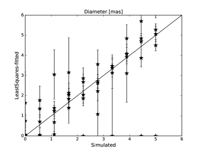
(a) Least squares-fitted diameter

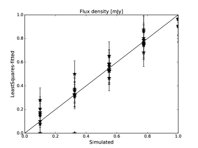
(b) Least squares-fitted flux density

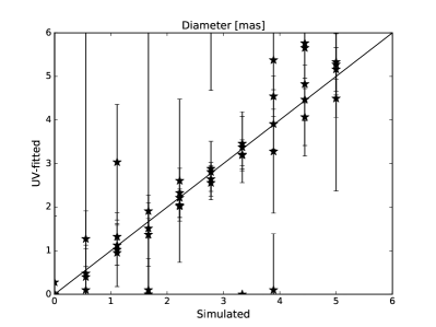
(c) UV-fitted diameter

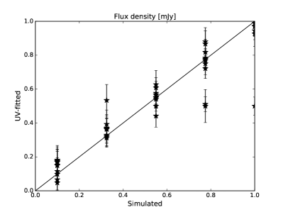
(d) UV-fitted flux density

Figure 11: Recovered diameters and flux densities for simulated data using three different methods: LS-fitting (first row) and UV-fitting (second row). The values for these figures are presented in Table 5. Cases where no fit was attempted in (at least one) method are included for completeness, but displaced as both value 0 and uncertainty 0 on the representative method axis.

Appendix E A comparison of source properties with published literature

In this section we present comparisons done between our fitted values for the compact sources and values available in the literature.

E.1 Source catalogues and completeness

To compare our results with previously published values we tried to match our detected sources with the positions published by Lonsdale et al. (1998, 2006); Parra et al. (2007); Batejat et al. (2011). The matching was done by comparing coordinates both automatically and manually to account for typos and blending effects, as mentioned in Sect. E.2, and in general the difference between our positions and the literature positions were much less than the beam size. When we found matches we have included the legacy name (for example W55, E8) in Tables 3 and 4. Even though we accounted for different reference positions, as noted in Sect. E.2, we found no counterpart in our images for the following sources: E4, E12, W3, W19, W24, W27. These may be false positives in previous studies, but it is also possible that they were weak when detected and has been declining since. Although we re-analyse the data used by for example Lonsdale et al. (2006), our images are not as deep as the ones previously published. Hence we may miss sources both in these old epochs due to the lower sensitivity, and in our recent 5 GHz epochs due to declining lightcurves and steep source spectra. Further investigation of these sources are beyond the scope of this work.

E.2 Positions of particular sources

As noted by Parra et al. (2007), the maser reference position assumed by Lonsdale et al. (2006) and previous studies was off by about $0.1^{\prime\prime}$ in declination, with a declination of $11.564^{\prime\prime}$ being assumed instead of $11.664^{\prime\prime}$, as noted above. However, from cross-referencing of the relative source positions listed in Table 1 of Lonsdale et al. (2006) with the positions obtained in this work, we find the reference position used for the relative coordinates listed by Lonsdale et al. (2006) at R.A. $15^{h}34^{m}57^{s}.26255$, Dec. $23^{\circ}30^{\prime}11^{\prime\prime}.352$, that is different from the maser peak position used for phase referencing. This difference has been taken into account when comparing positions and flux densities for these sources.

We note that the R.A. position listed by Lonsdale et al. (2006) for W11 corresponds to 57^s.2300, which is consistent with the position we find as well as the position listed by Batejat et al. (2011). However, in Parra et al. (2007) this source is listed with R.A. 57^s.2230 which seems to be a typographical error. Furthermore, the position listed for E11 by Lonsdale et al. (2006) corresponds to our source 0.2910+0.325, which is about 10 mas from the source 0.2195+0.335 (E10). However, we also find a source 0.2913+0.333 situated between these two sources, only about 3 mas from 0.2195+0.335. From Table 1, it is clear that observations at wavelengths longer than 6 cm do not have sufficient resolution to distinguish the two sources 0.2195+0.335 and 0.2913+0.333, and hence the flux densities measured at 1.4 GHz for these two sources, also in this work, should be interpreted with caution. We note that Batejat et al. (2011) associated 0.2913+0.333 with the previously listed source E11 instead of associating 0.2910+0.325 with E11 as we have done. Although 0.2195+0.335 and 0.2913+0.333 may be confused at 1.4 GHz, the resolution is good enough to separate 0.2913+0.333 and 0.2910+0.325. We therefore believe that Batejat et al. (2011) misidentified 0.2913+0.333 as E11, likely because 0.2910+0.325 is weaker at 6 cm than 0.2913+0.333, and hence their spectrum for E11 should be interpreted with caution.

To avoid typographical errors in this paper we have generated all figures and tables in the paper directly from the source catalogues generated by the source-finding algorithm as described in Sect. 2.1, without any manual editing.

E.3 Flux densities and sizes

As stated previously, some data included in this work have been published before. In Fig. 12, we compare the flux densities and sizes measured in this work with previously published values.

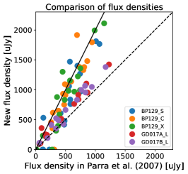
(a) Flux density vs Parra et al. (2007)

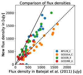
(b) Flux density vs Batejat et al. (2011)

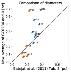
(c) Diameter vs Batejat et al. (2011)

Figure 12: Comparison of flux densities and sizes measured in this work with previously published values using the same data. The dashed lines indicate a one-to-one correspondence, and the solid lines indicate the new values to be a factor of 2 higher than the ones previously published. In Fig. 12(c), stars mark sources resolved at both bands by Batejat et al. (2011) (bold face in their Table 3) while circles mark the remaining sources. See Sect. E for a discussion of discrepancies.

Flux densities for the epochs GD017 and BP129 where reported by Parra et al. (2007), where the 18 cm values observed in 2003 (GD017A) were taken from Lonsdale et al. (2006). In Fig. 12 (panel a), we compare the flux densities recovered in this work to those previously published by Parra et al. (2007). We find that we in general find larger values, although the scaling factor varies between publications and data sets. Notably, we measure approximately two times higher flux densities than previously reported for all BP129. Since we find that our fitting method produces good results compared to for example manual inspection of the images (which was the method used to extract the flux densities by Parra et al. (2007) for BP129) we believe this flux discrepancy is due to differences in calibration and imaging strategy. However, a factor of two is much larger than expected given the uncertainties of the measurements. We use the same calibration strategy for BP129 as for other epochs. We have checked our calibration scripts for BP129 carefully without finding any reason for too high flux densities. We therefore suspect that values reported for BP129 by Parra et al. (2007) suffer from a systematic error in the calibration or imaging strategy, giving too low flux densities. We note that the image noise levels reported by Parra et al. (2007) are very similar to the noise we obtain. This argues against a simple difference in how the flux scale was set. Instead, such a flux density reduction suggests incoherent addition of visibilities, that is with strong phase errors present in one or more antennas during a significant period of time. We note that self-calibration could increase the flux density of sources in many epochs, which should reduce the RMS noise in the image. However, we see, for example for the GD017-epochs, an increase in both RMS noise level and source flux density compared to previous publication. Such an increase could instead be attributed to differences in amplitude calibration strategy, where our careful alignment of potentially bad antennas using bright sources should provide a more accurate amplitude scale. Further investigation of the details of the calibration performed by Lonsdale et al. (2006) and Parra et al. (2007) is beyond the scope of this paper.

Flux densities for epochs GC028 and GC031A are reported in Batejat et al. (2011), together with a revised version of the flux densities for the 6 cm data of BP129 (the 13 cm and 3.6 cm values for BP129 are taken directly from Parra et al. 2007). In Fig. 12 (panel b), we compare the flux densities recovered in this work to those previously published by Batejat et al. (2011). We find the flux densities reported for GC031A to be in excellent agreement with our measurements. However, we measure flux densities to be 1.5 times higher than reported for GC028 and BP129-C by Batejat et al. (2011). Again, using the same argument as in the previous paragraph, we assume that our new values are correct. We note that Batejat et al. (2011) claim an image noise of 41 $\mu$Jybeam^-1 for BP129-6 cm, which is a factor of two lower than what we obtain. We note that while Batejat et al. (2011) left multiple sources unclassified due to inconsistent lightcurves, we find, given our higher flux density values for some epochs, the lightcurves for these sources consistent with SNe/SNR evolution, as noted in Sect. E.4.

Source sizes were reported by Batejat et al. (2011) using data at 2 cm and 3.6 cm. In Fig. 12 (panel c), we compare the sizes given in Batejat et al. (2011) with our measurements from the same data. We only include the 12 sources where diameters are given in Table 3 of Batejat et al. (2011) that is not the sources with only upper limits. The sources fitted in both epochs by Batejat et al. (2011), that is bold face in their Table 3, are shown as stars in our Fig. 12, while the remaining sources are shown as circles. As new diameters, we take the average of the fitted values for the 2 cm and 3.6 cm images, as done by Batejat et al. (2011). We find the measurements to be in reasonable agreement.

E.4 Source classification changes

The number of sources detected in this work is too large for a detailed discussion on each object. However, in this section we discuss the classification of a few particular sources where previous studies have suggested AGN activity.

The source 0.2171+0.484 (W39) was left unclassified by Batejat et al. (2011) because it showed declining luminosity at long wavelengths and increasing luminosity at short wavelengths. After re-analysing the data, we find 0.2171+0.484 to have stable or declining lightcurves at all frequencies with a powerlaw spectrum, consistent with an SNR scenario where the blast wave is interacting with the ISM.

The source 0.2915+0.335 was also left unclassified by Batejat et al. (2011) as it showed declining luminosity at long wavelengths and increasing luminosity at short wavelengths. We instead find the lightcurves for 0.2915+0.335 to decline at both 6 cm and 3.6 cm, with approximately the same flux densities in both bands. Little or no emission is detected at 18 cm. The faint 18 cm emission and fact that the 6 cm emission is not significantly brighter than the 3.6 cm emission may indicate significant internal and/or external free-free absorption. Although 0.2915+0.335 is today declining at 6 cm and 3.6 cm, it emitted close to $1.5\times 10^{28}$ erg s^-1 Hz^-1 at these wavelengths in 2006. Given the relatively small measured size of 0.2 pc, the weak 18 cm emission, this source may be a relatively young SN where the shock is interacting with a dense ionised CSM.

Finally, the three sources 0.2306+0.502 (W10), 0.2241+0.520 (W17), and 0.2122+0.482 (W42), noted as flat-spectrum AGN candidates by Parra et al. (2007), are likely SNRs.

E.4.1 OH-maser sources

We note that in addition to the continuum sources, we also detect, in our 18 cm observations, three sources in OH-maser emission, without any continuum counterpart, at positions 0.2243+0.665, 0.2957+0.341, 0.2912+0.219. We identify these as the maser objects W1, E1, and E2 discussed by Lonsdale et al. (1998). These sources are however not included in Tables 3 and 4 as a discussion of the OH-maser emission in Arp 220 is beyond the scope of this work. We refer the interested reader to for example Lonsdale et al. (1998); Rovilos et al. (2003).

We note, however, that at the position of the OH-maser listed as W2 by Lonsdale et al. (1998), we find a clear (although relatively weak) continuum counterpart 0.2394+0.540 at multiple epochs and frequencies with stable or declining lightcurves. Based on the available data we conclude that this source is likely an SNR.

Appendix F Source summary slides

The 97 summary pages, one per source, are available in the online version of this paper. Each page shows the multi-frequency lightcurve, the source spectra taken from data points close in time, and the size measurements made in all epochs with sufficient resolution.

See pages - of figures/appendixE.pdf