Chiral vortical effect with finite rotation, temperature, and curvature

Abstract

We perform an explicit calculation of the axial current at finite rotation and temperature in curved space. We find that finite curvature and mass corrections to the chiral vortical effect satisfy a relation of the chiral gap effect, that is, a fermion mass-shift by a scalar curvature. We also point out that a product term of the angular velocity and the scalar curvature shares the same coefficient as the mixed gravitational chiral anomaly. We discuss possible applications of the curvature induced chiral vortical effect to rotating astrophysical compact objects described by the Kerr metric. Instead of direct calculation we assume that the Chern-Simons current can approximate the physical axial current. We make a proposal that the chiral vortical current from rotating compact objects could provide a novel microscopic mechanism behind the generation of collimated jets.

I Introduction

The chiral vortical effect (CVE) refers to the topological axial current induced by rotation of chiral matter. An analytical formula for the current has been originally derived microscopically for a Dirac matter distribution in a rotating frame Vilenkin:1978hb and applied to neutrino fluxes from rotating black holes Vilenkin:1979ui . More detailed calculations for general field theories were later reported in Ref. Vilenkin:1980zv . Interest in the CVE has been reignited by an analogous topological phenomenon called the chiral magnetic effect (CME) that refers to the generation of an electric current due to the axial anomaly in the presence of an external magnetic field (see Ref. Kharzeev:2013jha and contributions therein). From the analogy with the CME, we can naturally anticipate that angular momentum would induce a similar effect, i.e., a chiral vortical current along the rotation axis. With the rotation axis chosen along the $z$ direction, the chiral vortical current can be written, to linear order in the angular velocity $\omega$ and for massless fermions, as (see Ref. Kharzeev:2015znc for a recent review):

$$j_{R/L}^{z}=\pm\biggl{(}\frac{T^{2}}{12}+\frac{\mu_{R/L}^{2}}{4\pi^{2}}\biggr{)}\omega\;,$$ (1)

with $R/L$ indicating the right-handed and left-handed sectors separately. Anomalous hydrodynamics Son:2009tf , AdS/CFT correspondence Erdmenger:2008rm , chiral kinetic theory Stephanov:2012ki have all substantiated Eq. (1).

In Ref. Landsteiner:2011cp a conjecture relating the current (1) to the anomalies with gauge and gravitational fields has been proposed (see Ref. Basar:2013qia for related discussions). Based on the Kubo formula for the chiral vortical conductivity with metric perturbations in the framework of fluid dynamics Landsteiner:2011iq , it was shown that the coefficients of the chemical potential $\mu_{R/L}^{2}$ and of the temperature $T^{2}$ in Eq. (1) are respectively proportional to the chiral anomalies in the gauge and the gravitational sectors. It is not entirely clear whether this conjecture is true in general and it is even possible to have a $T^{2}$ part of the CVE even when there is no perturbative anomaly (see Refs. Golkar:2012kb ). However, the suggestion is intriguing as the non-vanishing transport coefficients appear as a manifestation of anomalies.

Generally it is not obvious whether the CVE is rooted in the mixed gravitational chiral anomaly or not, as the relation between the two may be quite indirect, as we will stress in the present work. So far, the established fact is that the coefficients appearing in the expression of the anomaly and in the chiral vortical current are common for some reason but this fact does not necessarily require that one can be derived from the other.

A way to clarify the situation would be to explicitly calculate gauge-invariant physical observables, namely, the axial current expectation value at finite rotation (with the angular velocity $\omega$), temperature $T$, and curvature (with the scalar curvature $R$), not resorting to the anomaly. Here we emphasize that a curved-space setup on top of the ordinary CVE at finite $T$ and $\omega$ provides between the CVE and the gravitational chiral anomaly, though, we do not insist on any precise relation between the CVE and the anomaly. Anticipating the step-by-step derivations of Sec. II, we shall write our final result down below:

$$j_{R/L}^{z}=\pm\biggl{(}\frac{T^{2}}{12}-\frac{m^{2}}{8\pi^{2}}-\frac{R}{96\pi^{2}}\biggr{)}\,\omega\,,$$ (2)

where $m$ is the fermion mass. For simplicity we dropped finite chemical potential terms $\propto\mu_{R/L}^{2}$, but it is not difficult to recover them. It is the last term $\propto R$ in Eq. (2) that would hint an indirect mechanism for the same coefficient as the chiral anomaly.

Beyond the formal significance in clarifying how thermal and geometrical effects mirror into each other, and how this impacts on the CVE formula, recently, it is of increasing interest to investigate the physics of relativistic rotating matter in heavy-ion collision experiments. Although the theoretical description of a spinning fluid is not yet fully understood Becattini:2009wh (see Ref. Becattini:2015tpl for recent discussions related to the present work), microscopic field-theoretical calculations are feasible. Rotating quark matter possibly created in heavy-ion collisions may accommodate a non-trivial phase diagram as described in Refs. Jiang:2016wvv ; Chernodub:2016kxh . In heavy-ion collisions, moreover, not only thermal effects but also those of strong magnetic fields play a critical role McLerran:2013hla . Then, as emphasized in Ref. Chen:2015hfc , an effective chemical potential associated with rotation would topologically induce a non-zero density Hattori:2016njk , which is one concrete manifestation of the chiral pumping effect Ebihara:2015aca . (As pointed out in Ref. Ebihara:2016fwa the partition function obtained in Ref. Chen:2015hfc encompassed such an induced density.) Because hot and dense matter created in heavy-ion collisions is rapidly expanding, a finite curvature associated with three dimensionally expanding geometries is expected to modify the above-mentioned estimates according to Eq. (2).

Another intriguing corollary of the above arguments is associated to the physics of astrophysical jets, whose formation mechanism (i.e., acceleration and collimation) is surrounded by many open questions. It is certainly an attractive idea to draw a connection between the CVE and the microscopic nature of jets from compact astrophysical sources, as discussed in the present work.

II Explicit Calculation

Our goal here is to compute the expectation value of the axial current in curved space directly using the propagator in a rotating system, i.e.,

$$j_{A}^{\mu}(x)=-i\lim_{x^{\prime}\to x}\text{tr}\bigl{[}\gamma^{\mu}\gamma_{5}S(x,x^{\prime})\bigr{]}\;.$$ (3)

Thus, all we need is the explicit form of the propagator $S(x,x^{\prime})$ at finite $T$ on the background of a rotating curved geometry. To construct the propagator, it is intuitively clearer to treat rotational and geometrical features separately.

We employ Riemann normal coordinates $\xi$ around a point $x$ (identified by $\xi=0$) and consider the coincident limit of the fermion propagator. Using Riemann normal coordinates significantly simplifies the analysis since the Christoffel symbols at $x$ are all vanishing and the Dirac matrices are just those in flat spacetime. A finite rotation $\omega$ can then be introduced as a small perturbation.

The coincident limit of the propagator in normal coordinates for $\omega=0$ takes the form,

$$S_{0}(x,x^{\prime}\to x)=\int\frac{d^{4}k}{(2\pi)^{4}}\,(-\gamma^{\mu}k_{\mu}+m)\,\mathcal{G}(k)\;.$$ (4)

Here $k$ is a momentum conjugate to $\xi$ and $\mathcal{G}(k)$ is a known function involving metric derivatives parker as

$$\mathcal{G}(k) =\Biggl{[}1-\biggl{(}A_{1}+iA_{1\alpha}\frac{\partial}{\partial k_{\alpha}}-A_{1\alpha\beta}\frac{\partial}{\partial k_{\alpha}\partial k_{\beta}}\biggr{)}\frac{\partial}{\partial m^{2}}$$

$$\qquad+A_{2}\biggl{(}\frac{\partial}{\partial m^{2}}\biggr{)}^{2}\Biggr{]}\frac{1}{k^{2}-m^{2}}+\cdots\;,$$ (5)

where $A_{1}$ represents a coefficient with mass-dimension 2 that is expressed in terms of Riemann tensors at $x$. Analogously, $A_{1\alpha}$ is a mass-dimension 3 coefficient, and $A_{1\alpha\beta}$, $A_{2}$ are mass-dimension 4 coefficients, involving spin operators. Explicit expressions for these coefficients can be found in Ref. parker . It is easy to argue by dimensional analysis that higher-order terms represented by the ellipses are suppressed at sufficiently high $T$, as we will explicitly see later.

For technical simplicity, in what follows we require two conditions to be satisfied. The first is that of stationarity, i.e., all metric components are time independent and the temporal components of the metric are space independent. We require this to utilize the standard Matsubara formalism valid for systems in thermal equilibrium. This condition may be relaxed at the price of using the more complicated real-time formalism to include thermal effects. We note that rotation induces a space-dependence in $g_{00}$ at $\omega^{2}$ order, but for our purposes it is necessary to go only to linear order in $\omega$. This is not a particularly restrictive assumption, since, for small $\omega$, we can always reduce the metric to a form compatible with this assumption by means of a conformal transformation.

The second condition we require is that all metric components are $z$ independent and the $z$ components of the metric are space independent. This condition corresponds to choosing the rotation axis along the $z$ direction, and removes the $z$ dependence of the spin operators of the rotation generators.

Thanks to the simplicity of Riemann normal coordinates, the calculations are straightforward. In this setup, the temporal direction is not distorted, and thus the propagator is a function of $t-t^{\prime}$. This allows us to define an energy conjugate to $t-t^{\prime}$ that is nothing but $k_{0}$ in Eq. (4). By applying the rotation generator, we can write the rotating propagator with $\boldsymbol{\omega}$ as

$$S(\boldsymbol{x},\boldsymbol{x}^{\prime},k_{0})=e^{\boldsymbol{\omega}\cdot\frac{1}{2}\boldsymbol{\Sigma}\frac{\partial}{\partial k_{0}}}S_{0}(\boldsymbol{x},\boldsymbol{x}^{\prime},k_{0})\;,$$ (6)

for $\boldsymbol{x}^{\prime}\sim\boldsymbol{x}$. (Note that $\boldsymbol{x}$ is the center of rotation, so that there is no orbital term.) Here, $\boldsymbol{\Sigma}$ is a spin operator defined by $\Sigma^{i}=\epsilon^{ijk}\frac{i}{4}[\gamma_{j},\gamma_{k}]$. Using our assumption of $\omega$ being small, we can proceed to expand in powers of $\omega$. To 0th order, we can replace $S(\boldsymbol{x},\boldsymbol{x}^{\prime},k_{0})$ with $S_{0}(\boldsymbol{x},\boldsymbol{x}^{\prime},k_{0})$. Then, using the symmetry properties of the Riemann tensors, we can readily convince ourselves that $j_{A}^{\mu}\bigr{|}_{\omega=0}=0$. This is expected: even in curved space the axial current is vanishing as long as there is no rotation.

To 1st order in $\omega$, the spin operator produces a difference leading to a non-zero Dirac trace. So, the whole quantity is proportional to $\text{tr}[\gamma_{5}\gamma^{\mu}\gamma^{\mu^{\prime}}\gamma^{\nu^{\prime}}\gamma^{\nu}]=4i\epsilon^{\mu\mu^{\prime}\nu^{\prime}\nu}$, a trait common to anomaly calculations. Some algebra gives

$$j_{A}^{\mu}=i\,\epsilon^{\mu\mu^{\prime}\nu^{\prime}\nu}\omega_{\mu^{\prime}\nu^{\prime}}\,\int\frac{d^{4}k}{(2\pi)^{4}}\,\frac{\partial}{\partial k_{0}}\,k_{\nu}\,\mathcal{G}(k)\;,$$ (7)

where we used a two-index representation of the angular velocity as $\omega^{i}=\epsilon^{ijk}\omega_{jk}$. Summation over the Matsubara frequencies $k_{0}$ is understood after the $k_{0}$ derivative is taken in the integrand. Using Eq. (5), we see that the first term returns the well-known formula of the CVE. That is, defining the energy dispersion $\varepsilon_{k}=\sqrt{\boldsymbol{k}^{2}+m^{2}}$, the CVE arises from

$$\begin{split}&\int\frac{d^{4}k}{(2\pi)^{4}}\frac{\partial}{\partial k_{0}}\frac{k_{0}}{k^{2}-m^{2}}=-i\int\frac{d^{3}k}{(2\pi)^{3}}\,n_{F}^{\prime}(\varepsilon_{k})\\ &=\frac{i}{\pi^{2}}\int_{0}^{\infty}dk\,\biggl{(}\varepsilon_{k}-\frac{m^{2}}{2\varepsilon_{k}}\biggr{)}\,n_{F}(\varepsilon_{k})\;,\end{split}$$ (8)

with $n_{F}(z)$ being the Dirac-Fermi distribution function. The integral above amounts to $\frac{i\Gamma(2)\zeta(2)}{2\pi^{2}}T^{2}=\frac{i}{12}T^{2}$ in the $m\to 0$ limit, from which we correctly arrive at Eq. (1).

The most interesting correction to the axial current emerges from the second term in Eq. (5). From textbook parker $A_{1}=R/12$, with the momentum integration being almost the same as the previous one apart from the mass derivative, we have:

$$\frac{\partial}{\partial m^{2}}\int\frac{d^{4}k}{(2\pi)^{4}}\,\frac{\partial}{\partial k_{0}}\,\frac{k_{0}}{k^{2}-m^{2}}=-\frac{i}{2}\int\frac{d^{3}k}{(2\pi)^{3}}\,\frac{n_{F}^{\prime\prime}(\varepsilon_{k})}{\varepsilon_{k}}\;.$$ (9)

In the $m\to 0$ limit the above integral yields $-i/(8\pi^{2})$. Therefore, together with the first term, the total current turns out to be

$$j_{A}^{z}=\biggl{(}\frac{T^{2}}{12}-\frac{m^{2}}{8\pi^{2}}-\frac{R}{96\pi^{2}}+\cdots\biggr{)}\,\omega\;,$$ (10)

in which neglected ellipses are higher order terms such as $R\,m^{2}/T^{2}$ for small $m$ and $R$. This proves our central result of Eq. (2). In the formula above, from Eq. (8), we inferred to lowest order the finite-$m$ corrections: $iT^{2}/12\to i(T^{2}/12-m^{2}/8\pi^{2})$. We note that, as we shall discuss shortly, at zero temperature and zero curvature, at linear order there should be no CVE and the above expression assumes $m^{2}\ll T^{2}$. Then, according to the chiral gap effect Flachi:2014jra , a finite scalar curvature shifts the fermionic mass gap as $m^{2}\to m^{2}+R/12$, which perfectly explains the ratio between the second and the third terms in Eq. (2). (See also Ref. Jensen:2012kj where the same term $\propto R\omega$ was obtained in a yet different way.)

It is also interesting to point out that the coefficient $1/12$ obtained, for instance in Refs. Landsteiner:2011cp ; Golkar:2012kb , is derived as the coefficient multiplying the scalar curvature term in the (heat-kernel) coefficient in Ref. Flachi:2014jra . This number, $1/12$, is independent of the background geometry.

We can continue the expansion to include higher-order corrections from Eq. (5). The next contribution leading to finite corrections seems to be $A_{1\alpha\beta}$. This term involves one more mass derivative,

$$\frac{\partial}{\partial m^{2}}\int\frac{d^{3}k}{(2\pi)^{3}}\,\biggl{[}\frac{n_{F}^{\prime\prime}(\varepsilon_{k})}{\varepsilon_{k}}+\frac{n_{F}^{\prime\prime\prime}(\varepsilon_{k})}{3}\biggr{]}\;\to\;-\frac{7\zeta(3)}{16\pi^{4}T^{2}}\;,$$ (11)

in the $m\to 0$ limit. It is non-trivial that the above combination of the integrals is infrared finite, though each has singularity. This adds a correction to the current by $\delta j_{A}^{\mu}=3\bar{A}_{100}\cdot 7\zeta(3)/(16\pi^{4}T^{2})$, where $\bar{A}_{1\alpha\beta}$ represents a part of $A_{1\alpha\beta}$ without spin operator  parker . However, n the present treatment with only static deformations, $\bar{A}_{100}$ is zero. Thus, the first non-zero correction appears from the second derivative in terms of $m^{2}$, that is,

$$\delta j_{A}^{z}=\bar{A}_{2}\cdot\frac{7\zeta(3)}{32\pi^{4}T^{2}}$$ (12)

with $\bar{A}_{2}$ being a mass-dimension 4 coefficient given by $\bar{A}_{2}=\frac{1}{120}{R_{;\mu}}^{\mu}+\frac{1}{288}R^{2}-\frac{1}{180}R_{\mu\nu}R^{\mu\nu}+\frac{1}{180}R_{\mu\nu\sigma\tau}R^{\mu\nu\sigma\tau}$. We stop here and will not include this correction in our considerations below.

Let us turn to intriguing features of the expansion. Explaining how a $T$-independent correction $\propto R$ in Eq. (2) appears from finite-$T$ calculations requires a delicate interchange of the two limits; $m\rightarrow 0$ and $T\rightarrow 0$. In fact, if we keep a finite $m$ and take the $T\rightarrow 0$ limit first, then we would have $\int\frac{d^{3}k}{(2\pi)^{3}}\,\varepsilon_{k}^{-1}n_{F}^{\prime\prime}(\varepsilon_{k})\to 0$, and no such term $\propto R$ survives, as we already noted. Therefore, the order of two limits, $T\to 0$ and $m\to 0$ is important. Here, we always assume the $m\rightarrow 0$ limit first and then vary $T$, as the value of $m$ defines the theory, while $T$ is a control parameter that we can adjust externally in physical situations.

One more comment is due. The above-mentioned calculations would be reminiscent of the high-$T$ expansion, but we emphasize that there is a crucial difference. If one performs the high-$T$ expansion for the pressure $p$ for example, the leading term is proportional to $T^{4}$, the next leading term $m^{2}T^{2}$, and the further next term $m^{4}$. The important point is that such $m^{4}$ term in the high-$T$ expansion is accompanied by a logarithmic singularity, $\ln(m/\pi T)$, which blows up for both $m\to 0$ and $T\to 0$. Unlike this, in the present case, such terms involving $\ln(m/\pi T)$ exactly cancel out, which can be also confirmed in the heat-kernel expansion. We remark that a logarithmic singularity with $R$ should vanish in odd spatial dimensions. These interesting observations might be related to the non-renormalization of the anomaly.

III Approximate Estimate of the Axial Current

For a more general geometry, beyond our simplifying assumptions, even up to linear order in $\omega$, the direct calculation of the axial current is impossibly difficult. We here propose to utilize as a proxy of the axial current the Chern-Simons current. As is well recognized, the Chern-Simons current is not gauge invariant, but we have empirically known that it can approximate the physical current, which is the case, for example, for the orbital component of the photon angular momentum. The CME is a well known example of the Chern-Simons current acquiring a physical significance thanks to an external chemical potential.

The chiral anomaly with gravitational background fields reads Kimura:1969 :

$$\nabla_{\mu}j_{A}^{\mu}=\frac{1}{384\pi^{2}}\epsilon^{\mu\nu\rho\lambda}R_{\mu\nu}^{~{}~{}~{}\alpha\beta}R_{\rho\lambda\alpha\beta}\,.$$ (13)

The right-hand side takes the form of a total divergence, from which the Chern-Simons current can be derived. In this way we can find the Chern-Simons current $j_{\rm CS}^{\mu}$ associated with the gravitational chiral anomaly as

$$j_{\rm CS}^{\mu}=\frac{1}{96\pi^{2}}\epsilon^{\mu\nu\rho\lambda}{\Gamma^{\alpha}}_{\nu\beta}\Bigl{(}\partial_{\rho}{\Gamma^{\beta}}_{\alpha\lambda}+\frac{2}{3}{\Gamma^{\beta}}_{\rho\sigma}{\Gamma^{\sigma}}_{\alpha\lambda}\Bigr{)}\;.$$ (14)

Under a coordinate transformation from $x^{\mu}$ to $x^{\prime\mu}$ with rotation, ${\Gamma^{k}}_{ij}$ acquire a correction by $(\partial x^{\prime k}/\partial x^{r})(\partial^{2}x^{r})/(\partial x^{\prime i}\partial x^{\prime j})$, that gives not only multiplicative transform but also additive shift as

$$\delta{\Gamma^{x}}_{0y}=-\delta{\Gamma^{y}}_{0x}=\omega\;.$$ (15)

Then, up to linear order in $\omega$, the Chern-Simons current takes the following form:

$$j_{\rm CS}^{\mu}=\frac{\omega}{48\pi^{2}}\bigl{(}{R^{0}}_{x0x}+{R^{0}}_{y0y}-{R^{x}}_{yxy}-{R^{y}}_{xyx}\bigr{)}\;.$$ (16)

The important observation here is that, once the $\omega$ dependence is extracted, the remaining part is written in terms of the Riemann tensors only. In our case, with flat $0$ and $z$ directions, only ${R^{x}}_{yxy}$ and ${R^{y}}_{xyx}$ survive, leading to the same expression as our direct calculation of Sec. II, $j_{A}^{z}=-\omega R/(96\pi^{2})$. This is a consistency check for our Ansatz of using the Chern-Simons current as a proxy of the directly calculated axial current.

The relation between the microscopically computed current and the Chern-Simons current should be understood in the same way as for the CME current. In the CME case, the axial current along the $z$ axis is proportional to $\epsilon^{z0ij}A_{0}\partial_{i}A_{j}$, which itself is gauge variant. However, once the chemical potential $\mu$ is turned on, $A_{0}$ is replaced with $\mu$, and then the rest part is the field strength tensor and thus gauge invariant; $\langle j_{A}^{z}\rangle\propto\mu B$ Fukushima:2008xe . In this way, the Chern-Simons current can be interpreted as a physical current due to the external environment. Our explicit calculations support the idea that the derivation of the CME based on the Chern-Simons current may hold also for the CVE involving the metric background with the following correspondence ($\mu$ in the CME) $\leftrightarrow$ ($\omega$ in the CVE).

At a glance one may feel not easy to upgrade the Chern-Simons current to a physical quantity. In the CME case the subtle point is how $\mu$ can be physical, while $A_{0}$ is not. The answer is that $\mu$ is a holonomy: $A_{0}$ itself can be gauged away but $\mu$ is a remainder that cannot be gauged away under the periodic boundary condition in the imaginary-time formalism. In fact it is well known that the Polyakov loop is a gauge invariant holonomy in non-Abelian gauge theories, and Abelian imaginary $\mu$ can be defined similarly in a gauge invariant way. For our problem with finite $\omega$, it can be gauged away by rotating coordinate transformation. We can, however, introduce an indelible $\omega$ imposing periodic boundary condition. This observation is consistent with the results in Ref. Hattori:2016njk ; Ebihara:2016fwa where it is argued that rotation alone cannot induce any physical consequence.

IV Astrophysical Jets from the Chiral Vortical Effect

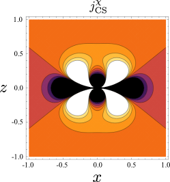
Figure 1: Axial current in the extremal limit in units of $\omega$. Light color represents positively large values and dark color represents negatively large values.

Once the above Ansatz of the Chern-Simons current as a proxy of the physical axial current is accepted, we have a powerful method to proceed to numerical computations. Let us consider a rotating gravitational background, described by the Kerr metric. It would be a complicated calculation to evaluate the propagator on the Kerr geometry, but it is rather straightforward to write the Chern-Simons current down. In Boyer-Lindquist coordinates ($t$, $r$, $\chi=\cos\theta$, $\phi$), after some calculations, we find $j_{\rm CS}^{r}\neq 0$ and $j_{\rm CS}^{\chi}\neq 0$, while $j_{\rm CS}^{0}=j_{\rm CS}^{\phi}=0$. Here, instead of showing the full expressions, let us discuss $j_{\rm CS}^{r}$ and $j_{\rm CS}^{\chi}$ in particular limits only. For small $\omega$, the current to linear order in $\omega$ reads,

$$j_{\rm CS}^{r}=\frac{3\pi(-3\pi+8rT_{B})\chi}{24576r^{6}T_{B}^{4}}\omega\;,\quad j_{\rm CS}^{\chi}=\frac{3\pi(-1+3\chi^{2})}{6144r^{6}T_{B}^{3}}\omega\;.$$ (17)

where $T_{B}$ is the black hole temperature (and not the thermodynamic temperature). If the thermodynamic temperature is involved, as discussed in Ref. Jensen:2012kj , spatial derivatives of the temperature would appear. In confronting the above expressions with the formula (1), we should remark that in Eqs. (17) both $T_{B}$ and $r$ are dimensionful quantities.

The angular dependence in the above results, $j_{\rm CS}^{r}\propto\chi=\cos\theta$, indicates the presence of a current aligned with the rotation axis. Coming back to the discussions in Ref. Vilenkin:1979ui , we can associate this axial current with neutrino flux. It is then tempting to interpret the present results in terms of a novel (sharing some similarities with the Penrose process Penrose ) microscopic mechanism for the generation of collimated astrophysical jets observed in rotating compact stellar objects (see Ref. Meier:2003bi ). Interestingly, it may be worth noticing that this mechanism would be generic to all rotating compact objects, and not limited to black holes.

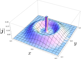
Figure 2: Axial current magnitude in the extremal limit at $z=0.2$ in units of $\omega$.

For astrophysical applications it is relevant to examine the extremal limit $T_{B}=0$. One may think, using expressions (17), that the limit $T_{B}\to 0$ would be singular. However, before the expansion in $\omega$, the limit smoothly exists. It should be noted that Eq. (17) gives the leading order term in an expansion in powers of $\omega/T_{B}$. Therefore, we cannot extrapolate Eq. (17) naively to $T_{B}\to 0$. The correct result for the leading $\omega$ order in the extremal limit is

$$j_{\rm CS}^{r} =-\frac{(1-2\xi)[\chi^{4}+4\chi^{2}\xi(3-8\xi)-48\xi^{3}(1-\xi)]\chi}{3\pi^{2}(\chi^{2}+4\xi^{2})^{5}}\omega^{3},$$ (18)

$$j_{\rm CS}^{\chi} =\frac{[\chi^{6}-\chi^{4}(3+56\xi^{2})+72\chi^{2}\xi^{2}(1+2\xi^{2})-48\xi^{4}]}{3\pi^{2}(\chi^{2}+4\xi^{2})^{5}}\omega^{4},$$ (19)

where $\xi=r\omega$. For clarity, we should remark that although the expansion for small $T_{B}$ and that for small $\omega/T_{B}$ do not commute, the limiting procedure is straightforward and does not pose any difficulty. It is interesting that these currents in the extremal limit become increasingly large for $\chi\to 0$ if $\omega$ (and $\xi$) is small enough. This feature is very different from Eq. (17). The currents in Eqs. (18) and (19) are plotted in Fig. 1, where we use the unit in terms of $\omega$ and we set $y=0$ without loss of generality due to the axial symmetry. It is not easy to imagine how the current is spatially distributed from Fig. 1, so the magnitude of the current is plotted in Fig. 2 which shows a 3D jet profile. As illustrated in these figures, the currents are strongly peaked near $z\sim 0$ or $\theta\sim\pi/2$. It is worth noting that heavy and slowly rotating objects generally exhibits such singular structures, implying that common compact stellar objects in the universe should be accompanied by a axial currents as displayed in Fig. 1. This result implies that the CVE currents may be a source for the surrounding disk as well as the astrophysical jets.

We note that Eqs. (18) and (19) are rapidly damping as $|\boldsymbol{j}|\propto r^{-5}$ at large distance. This is so because there is no given chiral charge and no net production of $j_{\rm CS}^{0}$ in this case. In other words the Kerr metric has $R=0$, so that the leading-order CVE term $\propto\omega R$ is vanishing. For a more qualitative estimate, we must assume a “freezeout” radius beyond which free particles are emitted out. In this work we will not go further into attempts to quantify our estimates using the Kerr metric. In reality black holes could be charged, and combinations with electromagnetic fields produce more contributing terms. Here, we point out a qualitative possibility and leave quantitative discussions including missing terms for the future.

It is an intriguing problem to discuss the physical implications of these currents for hot and dense quark matter in heavy-ion collisions as well as in astrophysics. In the same way as to interpret the chiral anomaly as parity-odd particle production Fukushima:2015tza , we can give a physical picture for these currents as extra contributions to phenomena similar to Hawking radiation (see Ref. Vilenkin:1979ui for discussions along these lines). Another interesting application includes anomalous neutrino transport in rapidly rotating system of black hole or neutron star mergers (see Ref. Yamamoto:2015gzz for an idea of anomalous neutrino transport in supernovae and Ref. Gorbar:2016klv for applications to the early universe).

V Conclusions

In this work we have calculated the axial current expectation value in curved space at finite temperature. The chiral vortical effect receives a correction proportional to the scalar curvature, $R$, which is consistent with the finite mass correction and the chiral gap effect. We point out that such a topologically induced current $\propto\omega R$ with $\omega$ being the angular velocity has the same overall coefficient as the Chern-Simons current. Our argument parallels that in the derivation of the chiral magnetic effect that is fully explained by the replacement of $A_{0}$ with the chemical potential $\mu$ in the Chern-Simons current. This physical augmentation of the Chern-Simons current due to the external environment offers an interesting theoretical device to approximate the particle production in non-trivial background geometries. We have adopted this Ansatz to use the Chern-Simons current as a proxy of the physical current to the case of a rotating astrophysical body and have argued that the chiral vortical current may provide a novel universal microscopic mechanism behind the generation of collimated jets from rotating astrophysical compact sources.

- (1) A. Vilenkin, Phys. Lett. 80B, 150 (1978).
- (2) A. Vilenkin, Phys. Rev. D 20, 1807 (1979).
- (3) A. Vilenkin, Phys. Rev. D 21, 2260 (1980).
- (4) D. Kharzeev, K. Landsteiner, A. Schmitt and H. U. Yee, Lect. Notes Phys. 871, pp.1 (2013).
- (5) D. E. Kharzeev, J. Liao, S. A. Voloshin and G. Wang, Prog. Part. Nucl. Phys. 88, 1 (2016).
- (6) D. T. Son and P. Surowka, Phys. Rev. Lett. 103, 191601 (2009).
- (7) J. Erdmenger, M. Haack, M. Kaminski and A. Yarom, JHEP 0901, 055 (2009).
- (8) M. A. Stephanov and Y. Yin, Phys. Rev. Lett. 109, 162001 (2012).
- (9) K. Landsteiner, E. Megias and F. Pena-Benitez, Phys. Rev. Lett. 107, 021601 (2011).
- (10) S. Golkar and D. T. Son, JHEP 1502, 169 (2015); S. Golkar and S. Sethi, JHEP 1605, 105 (2016).
- (11) G. Basar, D. E. Kharzeev and I. Zahed, Phys. Rev. Lett. 111, 161601 (2013).
- (12) K. Landsteiner, E. Megias, L. Melgar and F. Pena-Benitez, JHEP 1109, 121 (2011).
- (13) K. Jensen, R. Loganayagam and A. Yarom, JHEP 1302, 088 (2013); JHEP 1405, 134 (2014).
- (14) F. Becattini and L. Tinti, Annals Phys. 325, 1566 (2010).
- (15) F. Becattini and E. Grossi, arXiv:1511.05439 [gr-qc].
- (16) Y. Jiang and J. Liao, Phys. Rev. Lett. 117, no. 19, 192302 (2016).
- (17) M. N. Chernodub and S. Gongyo, JHEP 1701, 136 (2017).
- (18) L. McLerran and V. Skokov, Nucl. Phys. A 929, 184 (2014).
- (19) H. L. Chen, K. Fukushima, X. G. Huang and K. Mameda, Phys. Rev. D 93, no. 10, 104052 (2016)
- (20) K. Hattori and Y. Yin, Phys. Rev. Lett. 117, no. 15, 152002 (2016).
- (21) S. Ebihara, K. Fukushima and T. Oka, Phys. Rev. B 93, no. 15, 155107 (2016).
- (22) S. Ebihara, K. Fukushima and K. Mameda, Phys. Lett. B 764, 94 (2017).
- (23) L. Parker and D. Toms, “Quantum Field Theory in Curved Spacetime: Quantized Fields and Gravity,” Cambridge University Press (2009).
- (24) A. Flachi and K. Fukushima, Phys. Rev. Lett. 113, no. 9, 091102 (2014).
- (25) T. Kimura, Prog. Theor. Phys. 42, no. 5, 1191-1205 (1969).
- (26) K. Fukushima, D. E. Kharzeev and H. J. Warringa, Phys. Rev. D 78, 074033 (2008).
- (27) R. Penrose and R. M. Floyd, Nature Phys. Sci. 229, 177 (1971).
- (28) D. L. Meier, New Astron. Rev. 47, 667 (2003).
- (29) K. Fukushima, Phys. Rev. D 92, no. 5, 054009 (2015); N. Müller, S. Schlichting and S. Sharma, Phys. Rev. Lett. 117, no. 14, 142301 (2016).
- (30) N. Yamamoto, Phys. Rev. D 93, no. 6, 065017 (2016).
- (31) E. V. Gorbar, I. Rudenok, I. A. Shovkovy and S. Vilchinskii, Phys. Rev. D 94, no. 10, 103528 (2016).