Joint Routing, Scheduling and Power Control Providing Hard Deadline in Wireless Multihop Networks

Abstract

We consider optimal/efficient power allocation policies in a single/multihop wireless network in the presence of hard end-to-end deadline delay constraints on the transmitted packets. Such constraints can be useful for real time voice and video. Power is consumed in only transmission of the data. We consider the case when the power used in transmission is a convex function of the data transmitted. We develop a computationally efficient online algorithm, which minimizes the average power for the single hop. We model this problem as dynamic program (DP) and obtain the optimal solution. Next, we generalize it to the multiuser, multihop scenario when there are multiple real time streams with different hard deadline constraints.

I Introduction

The Telecommunication field is growing at a tremendous pace across the globe in the last few decades. The number of mobile users and mobile internet applications are growing exponentially [9]. Users are looking for various services such as voice calls, video calls, data and internet of things (IoT) applications. One of the reasons for such a high mobile user growth is that people are using mobile phones for their business purposes as well. The adoption of mobile technology by citizens of a country positively affects both the income of its citizens as well as the gross domestic product (GDP) of the country. At the same time growing carbon footprint of Telecommunication industry has been a cause of concern and green communications has been the goal of next generation cellular systems ([6], [35]). Thus, this paper addresses the question of providing Quality of Service (QoS) to real time applications while minimizing the transmit power.

A specific quality of service may be desired or required for certain types of network traffic [48]. For example, hard deadline may be needed for streaming media, internet protocol television (IPTV), Voice over IP (VoIP), video-conferencing, safety-critical applications such as remote surgery, and real-time control of machinery. However, for TCP file transfers and web browsing, a lower bound on the mean rate provided may be an appropriate QoS.

In the following we survey the related literature. [1] provided the power allocation policy for a single fading link which optimizes the rate. They ignored higher layer performance measures like queueing delay. Energy efficient scheduling under mean delay constraint was first addressed in ([3], [4]). Cross layer scheduling algorithms which stabilized a communication network were considered in ([7], [25], [27], [36], [37]). Algorithms which minimize mean delay were designed in [10].

[14] considered the problem of minimizing average delay under average power constraint, proved existence of an optimal policy and obtained structural results for the optimal policy. Near-optimal closed-form solution is obtained in [35] that minimizes the average queue length under average power constraint when the rate is a linear function of power. In [33] considered the problem of minimizing the average power under average queue constraint, and show the existence of an optimal policy. [32] implemented an online algorithm by modifying the value iteration equation that minimizes the average power under an average delay constraint for a single user. Existence of stationary optimal polices for the constrained average-cost Markov decision processes was shown by setting up the problem as a constrained Markov decision process (C-MDP) in ([2], [13], [38]). Using techniques in Markov decision process (MDP), structural properties of the optimal policy were obtained in [12].

[26] proposed a new innovative algorithm which optimizes power while satisfying an upper bound on the sum of the average queue lengths of multiple users by dropping packets intelligently. [42] proposed a suboptimal policy which minimizes the average power under average queue constraint when there is an upper bound on packet loss also. [43] obtained asymptotic lower bounds for average queue length and average power consumption. [28] presented an algorithm for a multiuser and multi channel scenario subject to an upper bound on the sum of the average queue length. To meet the constraints the algorithm needs to learn the system parameters.

Energy efficient schemes are proposed when there is a hard deadline constraint over a wireless fading channel in ([8], [20], [40], [44], [45]). [11] presented a policy which minimizes the energy for sending a fixed number of packets under given hard deadline delay constraints. These works studied the scenario when there is a energy harvesting system. [24] obtained a closed form optimal average power solution when the hard deadline is two and proposed a sub-optimal solution when the hard deadline constraint is more than two. [8] proposed an energy efficient scheduler with individual packet hard delay constraints. In [34] obtains optimal solution that minimizes the average power under hard deadline constraint, when the rate is a linear function of power.

Multihop QoS problem can be solved in either a distributed or a centralized manner. Work on joint routing, scheduling and power control was provided in [5] which maximizes a utility function under average power constraint. As this problem is intractable they provided a heuristic sub-optimal algorithm. [19] considered the problem of ensuring a fair utilization of network resources by jointly optimizing power control, routing, and scheduling and obtained an efficient sub-optimal solution. [15] extended the solution in [5] to a multihop network where different nodes have multiple antennas and presented an efficient algorithm for providing max-min fairness.

[17] uses quadratic Lyapunov functions to provide novel back-pressure algorithms. In [18], using the above approach upper bounds on average delay are presented. These back-pressure algorithms provide stability of the network if the load is within the capacity region. But under high load, the end-to-end delay will be large and may violate any mean delay constraints.

A distributed scheme for joint power control, scheduling and routing is proposed in ([21], [23], [46]) for wireless networks that guarantees the attainment of a certain fraction of the capacity region under the signal to interference ratio (SINR) model. Gossip algorithms are surveyed in [39]. In [22], authors proposed a distributed algorithm which uses a randomized approach to make provision for QoSs such as end-to-end mean delay/hard deadline delay. [41] proposes a distributed scheme, based on MDP, to ensure end-to-end hard deadline constraints.

Our contribution: We consider a multihop wireless network where the links experience fading. We have obtained closed-form solutions, that minimize the average power when there is a hard deadline constraint for a single user, single hop scenario. The problem is formulated as a dynamic program (DP). By observing the solution structure of the DP, we obtain an elegant closed-form expression for the optimal policy. Later on, we extend our single user, single hop hard deadline results to the single/multiuser, multihop scenario, when the rate is a logarithmic function of power and obtain computationally efficient algorithms when every user has its own end-to-end hard deadline constraint. We obtain efficient routing, scheduling and power control to provide end-to-end hard deadline for the users.

Our model is close to that of [24]. But [24] only considers a single user transmitting over one hop. They obtain optimal policy for a deadline of 2 slots only and obtain heuristics for higher deadline. In [41] multiuser and multihop hard deadline is considered. But there is no fading on the transmission links, no power control and the arrival processes are deterministic. In our case we consider channels with fading, arrival processes are random and optiomal power scheme is obtained. In [22] the above mentioned limitations of [41] are not there but it provides random routing and does not optimize power.

The paper is organized as follows. In Section II we describe the system model. In Section III we consider the system when data packets arrive to the queue periodically after $M$ slot intervals. Section IV considers the case when the data packets arrive in every slot of the frame and should be served by the end of the frame. In Section V we extend the results of single user, single hop to single user, multihop scenario. In Section VI we generalize the results to the case when multiple, real time streams arrive, each with its own hard delay constraint. Finally, Section VII concludes the chapter.

II System Model

Initially we consider a single user, single hop system. This will be later on generalized to a multiuser, multihop system.

We consider a discrete time queue, where time is divided into slots of duration one unit. Let $A_{k}$ nats arrive in the queue at the beginning of slot $k$ and they are stored in an infinite buffer. These should be transmitted within next $M$ slots (i.e., in time $[k,(k+M)))$, where $M<\infty$ is a positive integer (see Sections III and IV for arrival processes considered there). In a practical system, this corresponding to the case that multiple number of packets arrive and at the time of transmission these can be fragmented arbitrarly. In a wireless system, this is a common practice. We assume that the channel gain $H_{k}$ is constant over the duration of slot $k$ and take value in a finite set. If the channel gains take continuous values, e.g., Rayleigh distributed, these can be approximated well by quantization by taking $L$ large enough. The channel gain $H_{k}$ is known to the transmitter and receiver at time $k$. We assume $\{H_{k},\ k\geq 0\}$ is independent, identically distributed (iid). Let $R_{k}$ be the number of nats transmitted in slot $k$.

Let $q_{k}$ denote the number of nats in the buffer at time $k$. Then, the queue evolves as,

$$q_{k+1}=(q_{k}+A_{k}-R_{k})^{+},\ k\geq 0,$$ (1)

where ${(x)}^{+}=\max(0,x)$. In slot $k$, the power required $P_{k}$ to transmit $R_{k}$ (nats) is given by Shannon formula,

$$R_{k}=\ln(1+\frac{\gamma P_{k}H_{k}}{\sigma^{2}}),$$ (2)

where $\ln$ denotes $\log$ with base $e$, $\sigma^{2}$ is the noise variance and $\gamma$ depends on modulation and coding used. Our objective is to minimize,

$$\limsup_{n\rightarrow\infty}\frac{1}{n}\sum_{k=1}^{n}E[P_{k}],$$ (3)

when there is an individual delay constraint on each packet, i.e., $A_{k}$ should be transmitted by time $(k+M),\forall k$.

In Section III we obtain the optimal policies where the time axis is divided into frames of size $M$ time units (first frame is $[1,M]$), where $M$ is the deadline of each packet. The arrivals come in the beginning of a frame. In Section IV we allow the packets to arrive in every slot but the packets arriving in time $[1,M]$, need to be transmitted by time $M$. The policies obtained in Sections III and IV will be used in later sections to deveop routing, scheduling and power control policies in multihop wireless networks providing end-to-end hard deadlines.

III Arrivals in Beginning of Frame

For simplicity, in Shannon formula (2), we assume $\sigma^{2}=1$, and $\gamma=1$. Our optimal policies obtained below can be generalized easily. We assume that $A_{k}$ nats arrive at time $kM+1$, $k=0,1,2,...$ and need to be transmitted by time $(k+1)M$. No other arrivals come in the mean time. We assume $\{A_{kM},k\geq 0\}$ is an $iid$ sequence. We provide an algorithm for this setup. It uses Dynamic Programming [30]. The intervals $[kM+1,(k+1)M]$ will be called frames of size $M$. The following theorem will be used to obtain the optimal algorithm below.

Theorem 1.

The optimal average power consumption

$$E_{H}[W_{M}(A_{1},H)]=Me^{\frac{A_{1}}{M}}\left(\displaystyle{\prod_{j=1}^{M}}E\left[\frac{1}{H^{\frac{1}{j}}}\right]^{\frac{j}{M}}\right)$$

$$-ME\left[\frac{1}{H}\right],$$ (4)

for $M\geq 1$.

Proof.

We define the set of all feasible policies $S_{M}({A_{1}})=\{R=(R_{1},...,R_{M}):\sum_{k=1}^{M}R_{k}=A_{1},R_{k}\geq 0,\forall k\}$. The expected cost for choosing policy $R$ is

$${W_{M}(A_{1},R,H)=E_{H}\left[\sum_{k=1}^{M}f(R_{k},q_{k},H_{k})\right],}$$ (5)

where $f(R_{k},q_{k},H_{k})$, the power consumed in slot $k$ by transmitting $R_{k}$ nats when $q_{k}$ is the queue length in slot $k$, is

$${f(R_{k},q_{k},H_{k})=\left(\frac{e^{R_{k}}-1}{H_{k}}\right)\text{ for }{\{R_{k}\leq q_{k}\}},\forall k}.$$ (6)

Our aim is to find a policy $R^{*}\in S_{M}(A_{1})$ for each $M\in\mathbb{N}$ for which

$$W_{M}(A_{1},H)\triangleq\inf_{R\in S_{M}(A_{1})}W_{M}(A_{1},R,H).$$ (7)

We define for any $1\leq j\leq M$, the average power spent from decision time $j$ onwards as

$${W_{M-j}(q_{j},h_{j})=E_{H}\bigg{[}\sum_{l=j}^{M}f(R_{l},q_{l},H_{l})\bigg{]},\text{where }q_{j}=\sum_{l=j}^{M}R_{l}.}$$ (8)

From Bellman’s equation ([16], [30]), we have $W_{M-j}(q_{j},h_{j})=$

$$\min_{R^{*}_{j}\in[0,q_{j}]}\left\{f(R_{j},q_{j},h_{j})+E_{H_{j+1}}[W_{(M-j-1)}(q_{j+1},H_{j+1})]\right\}.$$ (9)

We obtain a closed-form solution using induction. Initially, we assume that the hard deadline constraint is one slot. Then, we need to transmit $A_{1}$ in the first slot itself. Let $h_{1}$ be the channel gain in slot $1$. Then power consumption in the first slot is $W_{1}(A_{1},h_{1})=\frac{e^{A_{1}}-1}{h_{1}}$. Hence the average power consumption is

$$E_{H}[W_{1}(A_{1},H)]=(e^{A_{1}}-1)E\left[\frac{1}{H}\right].$$ (10)

Thus, (1) is satisfied for $M=1$.

Let for $M\geq 1$,

$$E_{H}[W_{M}(A_{1},H)]=Me^{\frac{A_{1}}{M}}\left(\displaystyle{\prod_{j=1}^{M}}E\left[\frac{1}{H^{\frac{1}{j}}}\right]^{\frac{j}{M}}\right)-ME\left[\frac{1}{H}\right].$$ (11)

Now,we want to show that (1) also holds for $M+1$. From (9),

$$W_{M+1}(A_{1},h_{1})= \min_{R_{1}}\left\{\frac{e^{R_{1}}-1}{h_{1}}+E_{H}[W_{M}(A_{1}-R_{1},H)]\right\}$$

$$= \min_{0\leq R_{1}\leq A_{1}}\Biggl{\{}\frac{e^{R_{1}}-1}{h_{1}}+Me^{\frac{A_{1}-R_{1}}{M}}\times$$

$$\bigg{(}\displaystyle{\prod_{j=1}^{M}}E\left[\frac{1}{H^{\frac{1}{j}}}\right]^{\frac{j}{M}}\bigg{)}-ME\left[\frac{1}{H}\right]\Biggr{\}}.$$ (12)

By taking derivate w.r.t $R_{1}$ and equating to zero. We get,

$$e^{R_{1}}=(h_{1})^{\frac{M}{M+1}}e^{\frac{A_{1}}{M+1}}\left(\prod_{j=1}^{M}\left(E\left[\frac{1}{H^{\frac{1}{j}}}\right]\right)^{\frac{j}{M+1}}\right).$$ (13)

Substituting (13) in (12).

$$W_{M+1}(A_{1},h_{1}) = \frac{(M+1)e^{\frac{A_{1}}{M+1}}\left(\displaystyle{\prod_{j=1}^{M}}E\left[\frac{1}{H^{\frac{1}{j}}}\right]^{\frac{j}{M+1}}\right)}{(h_{1})^{\frac{1}{M+1}}}$$ (14)

$$- ME\left[\frac{1}{H}\right]-\frac{1}{h_{1}}.$$

By taking expectation of the above equation on both side. We get

$$E_{H}[W_{M+1}(A_{1},H)]=(M+1)e^{\frac{A_{1}}{M+1}}\left(\displaystyle{\prod_{j=1}^{M+1}}E\left[\frac{1}{H^{\frac{1}{j}}}\right]^{\frac{j}{M+1}}\right)$$

$$-(M+1)E\left[\frac{1}{H}\right].$$

∎

From Theorem 1, if $A_{1}$ data is to be transmitted in a frame of size $M$, then in slot $k$, $1\leq k\leq M$, the data transmitted $R_{k}$ with remaining deadline of $M-k$ is

$${R_{k}=\ln\left((h_{k})^{\frac{M-k-1}{M-k}}e^{\frac{A_{1}}{M-k}}\left(\prod_{j=1}^{M-k-1}\left(E\left[\frac{1}{H^{\frac{1}{j}}}\right]\right)^{\frac{j}{M-k}}\right)\right)}.$$ (15)

All our derivations hold good for continuous channel case as well. We should replace the summations over the channel gains with the integrations over the channel distributions.

From (1), we see that $W_{M}(A_{1},h_{1})$ is exponentially increasing in $A_{1}$. Also, since the policies for $M$ are a subset of policies for $M+1$, $E_{H}[W_{M+1}(A_{1},H)]<E_{H}[W_{M}(A_{1},H)]$. We can indeed prove that this inequality can be made strict.

For the non-fading case, i.e., $H_{k}=1$. Hence, from (III) we get

$$R_{k}=\displaystyle{\frac{A_{1}}{M},\ \forall k,\ 1\leq k\leq M.}$$ (16)

We summarize this algorithm as Algorithm 1 below. We initialize the hard deadline constraint as $D_{1}=M$, $q_{1}=0$ and place the data in the queue and queue evolves as $q_{k}=q_{k}+A_{k}1_{\{(k-1)\mod M=0\}}$. It should be served within next $M$ slots including the current slot of the arrival. In slot $k$, we transmit $R_{k}=\ln\left((h_{k})^{\frac{D_{k}-1}{D_{k}}}e^{\frac{q_{k}}{D_{k}}}\left(\prod_{j=1}^{D_{k}-1}\left(E\left[\frac{1}{H^{\frac{1}{j}}}\right]\right)^{\frac{j}{D_{k}}}\right)\right)$ and we also update the queue length as $q_{k+1}=\left(q_{k}-R_{k}\right)$. We update the remaining hard deadline as $D_{k+1}=D_{k}-1+M1_{\{(k-1)\mod M=0\}}$. We run this algorithm in every slot, where $T$ is the total number of frames.

  1. Initialize $D_{1}=M$ and $q_{1}=0$

  2. for $k=1:1:TM$

  (i) $q_{k}=q_{k}+A_{k}1_{\{(k-1)\mod M=0\}}$

  (ii) Let $h_{k}$ be the instantaneous channel gain in time slot $k$.

  (iii) Compute ${R_{k}=\ln\left((h_{k})^{\frac{D_{k}-1}{D_{k}}}e^{\frac{q_{k}}{D_{k}}}\left(\prod_{j=1}^{D_{k}-1}\left(E\left[\frac{1}{H^{\frac{1}{j}}}\right]\right)^{\frac{j}{D_{k}}}\right)\right)}$

  (iv) Update $q_{k+1}=\left(q_{k}-R_{k}\right)$

  (v) Update $D_{k+1}=D_{k}-1+M1_{\{(k-1)\mod M=0\}}$

  endfor

Algorithm 1 Average Power Optimal for hard deadline, when the rate is concave function of power

Now, we compare our optimal policy with the heuristic policies proposed in [24]. $A_{k}$ takes values from the set $\{0.5,1,1.5\}$ with equal probabilities. Channel gains take values in the set $\{0.25$, $0.37$, $0.5$, $0.62\}$ with equal probabilities. Data comes only at the beginning of the frame and should be served by the end of the frame. The duration of the frame is $M$ slots. We plot the optimal average power and the power consumed by the heuristic schemes in ([8], [24]) in Fig. 1. It is clear that the average power consumption decreases with the hard deadline $M$ and our scheme outperforms the other schemes in ([8], [24]).

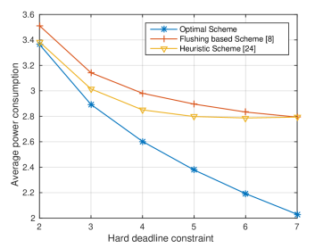
Figure 1: Average power consumption of optimal scheme and proposed heuristic schemes in [24] and [8] vs hard deadline constraint $M$.

IV Data Arrives in Every Slot

In this Section, we consider the case when the data arrives in every slot of the frame and all the data which has arrived in the frame should be served by the end of the frame. We assume that $\{A_{k},k\geq 2\}$ is iid. In the beginning of the frame we have data $\bar{A}_{1}$, independent of $\{A_{k},k\geq 2\}$. Distribution of $\bar{A}_{1}$ can be different from that of $A_{2}$.

The following theorem will provide us the algorithm. This is an extension of Theorem 1.

Theorem 2.

Let the data arrive in every slot of the frame and the data arriving between $[kM+1\ (k+1)M]$, should be served by $(k+1)M$. Also, let $\bar{A}_{1}$ nats be there in the beginning of slot $1$. Then, the average power consumption for the optimal solution is,

$$E_{{A_{2}},H}[W^{\prime}(\bar{A}_{1},H)]=Me^{\frac{\bar{A}_{1}}{M}}\left(\displaystyle{\prod_{j=1}^{M}}E\left[\frac{1}{H^{\frac{1}{j}}}\right]^{\frac{j}{M}}\right)$$

$$\left(\prod_{j=1}^{M-1}E_{A_{2}}\left[e^{\frac{A_{2}}{j}}\right]^{\frac{j}{M}}\right)-ME\left[\frac{1}{H}\right],$$ (17)

for all $M\geq 1$.

Proof.

When the frame size is one, we have

$$E_{H}[W^{\prime}_{1}(\bar{A}_{1},H)]=(e^{\bar{A}_{1}}-1)E\left[\frac{1}{H}\right].$$ (18)

Thus, (2) is satisfied. Let it be satisfied for $M\geq 1$. We show it for $M+1$. By (9),

$$W^{\prime}_{M+1}(\bar{A}_{1},h_{1}) = \min_{0\leq R_{1}\leq\bar{A}_{1}}\biggl{\{}\frac{e^{R_{1}}-1}{h_{1}}$$

$$+ E_{H}E_{A_{2}}[[W^{\prime}_{M}(\bar{A}_{1}-R_{1}+A_{2},H)]]\biggr{\}}.$$

By taking derivate w.r.t. $R_{1}$ and equating to zero. We get

$$e^{R_{1}}=(h_{1})^{\frac{M}{M+1}}e^{\frac{\bar{A}_{1}}{M+1}}\left(\prod_{j=1}^{M}E\left[\frac{1}{H^{\frac{1}{j}}}\right]^{\frac{j}{M+1}}\right)\times$$ (20)

$$\left(\prod_{j=1}^{M}E_{A_{2}}\left[e^{\frac{A_{2}}{j}}\right]^{\frac{j}{M+1}}\right).$$

Substituting (20) in (IV) and taking expectation over $H$, we get

$$E_{A_{2},H}[W^{\prime}_{M+1}(\bar{A}_{1},H)]=(M+1)e^{\frac{\bar{A}_{1}}{M+1}}\times$$

$$\left(\displaystyle{\prod_{j=1}^{M+1}}E\left[\frac{1}{H^{\frac{1}{j}}}\right]^{\frac{j}{M+1}}\right)\left(\prod_{j=1}^{M}E_{A_{2}}\left[e^{\frac{A_{2}}{j}}\right]^{\frac{j}{M+1}}\right)$$

$$-(M+1)E\left[\frac{1}{H}\right].$$ (21)

∎

This gives the following Algorithm 2. We initialize the hard deadline constraint as $D_{1}=M$, $q_{1}=0$ and set $q_{k}=q_{k}+A_{k}$, where $q_{1}=0$. In time slot $k$, we transmit

$$R_{k}=\ln\Biggl{(}e^{\frac{q_{k}}{D_{k}}}(h_{k})^{\frac{D_{k}-1}{D_{k}}}\bigg{(}\prod_{j=1}^{D_{k}-1}E\left[\frac{1}{H^{\frac{1}{j}}}\right]^{\frac{j}{D_{k}}}\bigg{)}\times$$

$$\bigg{(}\prod_{j=1}^{D_{k}-1}E_{A_{2}}\left[e^{\frac{A_{2}}{j}}\right]^{\frac{j}{D_{k}}}\bigg{)}\Biggr{)}$$

and we update the queue length as $q_{k+1}=(q_{k}-R_{k})$ and $D_{k+1}=D_{k}-1$. We run this algorithm in every frame.

  1. Initialize $D_{k}=M$, $q_{1}=0$

  2. for $k=1:1:TM$

  (i) $q_{k}=q_{k}+A_{k}$(ii) Let $h_{k}$ is instantaneous channel gain in time slot $k$. (iii) Compute $R_{k}=$$\ln\left(e^{\frac{q_{k}}{D_{k}}}h_{k}^{\frac{D_{k}-1}{D_{k}}}\Pi_{j=1}^{D_{k}-1}E\left[\frac{1}{H^{\frac{1}{j}}}\right]^{\frac{j}{D_{k}}}\left(\Pi_{j=1}^{D_{k}-1}E\left[e^{\frac{A}{j}}\right]^{\frac{j}{D_{k}}}\right)\right)$(iv) Update $q_{k+1}=(q_{k}-R_{k})$ (v) Update $D_{k+1}=(D_{k}-1)+M1_{\{(k-1)\mod M=0\}}$

  endfor

Algorithm 2 Data comes in whole frame

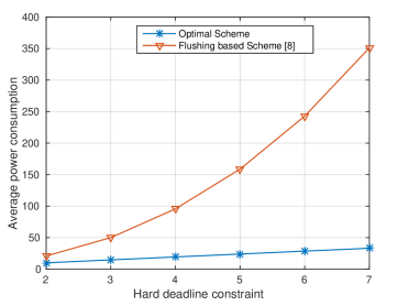
Figure 2: Average power consumption vs hard deadline constraint.

From the expression (2) for $W^{\prime}_{M}(\bar{A}_{1},h_{1})$ we observe that the power consumed exponentially increases with $\bar{A}_{1}$. But unlike, the results in Section III, $E_{A_{2},H}[W^{\prime}_{M}(\bar{A}_{1},H)]$ increases with $M$ if $\bar{A}_{1}$ and $A_{2}$ have the same distribution. This is because there is traffic arriving during the frame itself. To see this, let for the case of frame size, $M+1$, in slot $1$, we use power $P_{1}$ and transmit $R_{1}$ nats, then

$$E_{{A}_{2},H}[W^{\prime}_{M+1}(\bar{A}_{1},H)]=P_{1}+$$

$$E_{{A}_{2},H_{1}}[W_{M}^{\prime}(\bar{A}_{1}+A_{2}-R_{1},H)]\geq E_{{A}_{2},H}[W^{\prime}_{M}(\bar{A}_{1},H)].$$

If $\bar{A}_{1}$ and $A_{2}$ have different distributions then this inequality may not hold because $\bar{A}_{1}+A_{2}-R_{1}$ may not be stochastically greater than $\bar{A}_{1}$.

Now, we compare our optimal policy with the algorithm proposed in [8]. Arrival process takes values from the set $\{2,2.5,3\}$ with equal probabilities. Channel gains take values in the set $\{0.5,0.75,1,1.25\}$ with equal probabilities. We have run the algorithm and plotted the simulated curves for average power consumptions versus the deadline constraint M in Fig. 2. Our algorithms always outperforms the algorithm in [8] and often substantially.

V Single User, Multihop Network

We consider a network which is a connected, directed graph $\mathcal{G(N,L)}$, where $\mathcal{N}$ is the set of nodes and $\mathcal{L}$ is the set of directed links. A subset of nodes (called source nodes) in the network transmits data to another subset of nodes (called destination nodes). Each source has one destination. The time axis is slotted. The stream of packets transmitted from a source node to its respective destination node is called a flow.

The set of user flows $\{1,2,\ldots,N\}$ is denoted by $\mathcal{F}$. Let $A^{f}_{k}$ be the number of nats generated by flow $f$ in slot $t$ at its source. We assume $\{A^{f}_{k},\ k\geq 0\}$ to be iid, independent for different flows. We will also assume $E[A^{f}]<\infty$ for each $f$. End-to-end hard deadline for flow $f$ is denoted as $D^{f}$.

We assume that when a node is transmitting to some other node, it cannot receive data from any other node(s). Similarly, when a node is receiving data from a node, it cannot transmit data to any other node. Other transmission constraints can be included in our setup (also, we can modify the setup to we allow fewer constraints, e.g., we allow full duplex links).

Because of these constraints we can divide the set of links $\mathcal{L}$ into independent sets. All links in a set can transmit at the same time, causing negligible interference to each other. However, the links in two different sets cannot transmit in the same slot. Efficient algorithms to obtain independent sets in a graph are available in [31].

Let $(i,j)$ be the link which connects node $i$ to node $j$. Let the channel gain in slot $k$ for link $(i,j)$ be $H_{ij}^{k}$, which is available to the nodes $i$ and $j$ at the beginning of slot $k$. We assume that the channel gain $H_{ij}^{k}$ remains constant during slot $k$. We also assume that the channel gain process $\{H_{ij}^{k},\ k\geq 0\}$ is iid on all links and independent for different links. The channel gain $H_{ij}^{k}$ takes values on a finite set. If in time slot $k$, the power spent by node $i$ for flow $f$ is $P_{ij}^{k}(f)$ then the data $R_{ij}^{k}(f)$ transmitted to node $j$ for flow $f$ is,

$$R_{ij}^{k}(f)=\frac{1}{2}\ln(1+\gamma_{ij}P_{ij}^{k}(f)H_{ij}^{k}/\sigma^{2}_{ij}),$$ (22)

where $\sigma^{2}_{ij}$ is the receiver noise variance and $\gamma_{ij}$ is a constant that depends on the modulation and coding used. For simplicity, we assume that $\sigma^{2}_{ij}=1$, and $\gamma_{ij}=1,\forall i,j$.

In this section, we consider the problem of a single user. For simplicity, from now onwards, in this section we will remove $f$ from the notation. Our objective is to minimize the overall average power consumption of the wireless network subject to the end-to-end deadline for all packets. We will use Algorithms 1 and 2, to solve the single user problem.

Suppose for the flow, the overall end-to-end hard deadline is $D$ slots. If we selected a path $\mathcal{P}$ for this flow with links $l_{1},l_{2},\cdots,l_{N_{1}}$, we can split the hard deadline $D$ into deadlines $D_{i},i=1,\cdots,N_{1}$ for each of the links such that $D_{i}\geq 1$ and $\sum_{i=1}^{N_{1}}D_{i}\leq D$. We should choose $D_{i}$’s such that the overall power required $\sum_{i=1}^{N}P_{i}$ on these links is minimized where $P_{i}$ is the power spent on link $l_{i}$. The power $P_{i}$ required on these links is obtained from Theorem 2 (for the source node 1) and Theorem 1 for the other nodes.

The link scheduling is done via TDMA on the independent sets. If there are $N_{2}$ independent sets in the graph, we retain only the independent sets in which at least one of the links on $\mathcal{P}$ resides (for multiuser scenario, we may have to consider all independent sets). For simplicity, we assume that link $i$ is in set $S_{i}$. We assign $D_{i}$ consecutive slots to set $S_{i}$. Also we assume that these links get their slots one after another on $\mathcal{P}$. Furthermore, we also assume that a link is in only one of the independent sets. Our procedure can be adapted to the general case. However a set $S_{i}$ will often have multiple links. Thus, we will consider the case where we take a route $\mathcal{P}$ where link $i$ has deadline $D_{i}$ and we assign $D_{i}$ consecutive slots to the set $S_{i}$. We will not insist that $\sum_{j=1}^{N_{i}}D_{j}=D$. We will in fact see that often $\sum_{j=1}^{N_{i}}D_{j}<D$ will provide less power, something which seems counterintuitive. Let there be $N_{3}$ independent sets needed for the links $l_{1},l_{2},\cdots,l_{N_{1}}$.

In this setup, node 1 will transmit for $D_{1}$ consecutive slots and then wait for $D2+D_{3}+\cdots+D_{N_{3}}$ slots for other independent sets to transmit and then again transmit for $D_{1}$ slots and so on. During these $D_{1}$ slots, it will get $A_{1},\cdots,A_{D_{1}}$ iid nats for transmission. Also it will have $\sum_{k=1}^{D_{2}+\cdots+D_{N_{3}}}A_{k}$ nats in the beginning of each of its frames (of size $D_{1}$ slots) generated by the source when it is not transmitting, for transmission. Thus by Theorem 2, the energy needed by node 1 to transmit all this data in a frame of size $D_{1}$ is given

$$=E_{A_{1},H}\left[W^{\prime}_{D_{1}}\left(\sum_{k=1}^{D_{2}+\cdots+D_{N_{3}}}A_{k},H\right)\right]$$ (23)

$$=D_{1}E[e^{\frac{A_{1}}{D_{1}}}]^{D_{2}+\cdots+D_{N_{3}}}\biggl{(}a_{D_{1}}\biggr{)}\left(\prod_{j=1}^{D_{1}-1}E[e^{\frac{A_{1}}{j}}]^{\frac{j}{D_{1}}}\right)$$

$$-D_{1}E\left[\frac{1}{H_{1}}\right],$$

where $a_{D_{i}}=\prod_{z=1}^{D_{i}}E\left[\frac{1}{H_{i}^{\frac{1}{z}}}\right]^{\frac{z}{D_{i}}}.$

For node 2 on the path, all the data it will transmit in its frame comes at the beginning of its frame of size $D_{2}$ slots. The data arriving is $\sum_{k=1}^{D_{1}+\cdots+D_{N_{3}}}A_{k}$. Hence, by Theorem 1, the energy required to transmit it is

$$E_{H}\left[W_{D_{2}}\left(\sum_{k=1}^{D_{1}+\cdots+D_{N_{3}}}A_{k},H\right)\right]$$

$$=D_{2}E\left[e^{(\sum_{k=1}^{D_{1}+\cdots+D_{N_{3}}}A_{k})/D_{2}}\right]\biggl{(}a_{D_{2}}\biggr{)}-D_{2}E\left[\frac{1}{H_{2}}\right]$$ (24)

Similarly for node $i$ on the path $\mathcal{P}$, we have $D_{i}$ slots in its frame and data $\sum_{k=1}^{D_{N_{3}}}A_{k}$ arrives only in the beginning of its frame. Thus the energy used is

$$E_{H}\left[W_{D_{i}}\left(\sum_{k=1}^{D_{1}+\cdots+D_{N_{3}}}A_{k},H\right)\right]$$

$$=D_{i}E\left[e^{(\sum_{k=1}^{D_{1}+\cdots+D_{N_{3}}}A_{k})/D_{i}}\right]\biggl{(}a_{D_{i}}\biggr{)}-D_{i}E\left[\frac{1}{H_{i}}\right]$$ (25)

Now we look at the power (23) and (25) to see what could possibly be good deadlines $D_{i}$. In (23), we see as $D_{1}$ increases, keeping $D_{2},\cdots,D_{N_{3}}$ same, $a_{D_{1}}$ decreases; $-D_{1}E\left[\frac{1}{H_{1}}\right]$ will also reduce power. But in the first term, some of the subterms increase. However, we will see that the dominant term is $E[e^{\frac{A_{1}}{D_{1}}}]^{D_{2}+\cdots+D_{N_{3}}}$. This exponentially decreases in $D_{1}$ and its effect is amplified by exponent $D_{2}+\cdots+D_{N_{3}}$. Thus as $D_{1}$ increases while other $D_{i}$s stay constant, we expect that power spent at node 1 will decrease. On the other hand if any of the other $D_{i}$’s increase, its power requirement will exponentially increase.

Now we look at (25) for node $i$. If $D_{i}$ increases but other $D_{j}$ are fixed, then $a_{D_{i}}$ decreases. Also $E[e^{A_{1}/D_{i}}]$ decreases and its effect is amplified by power $D_{i}$. Thus, we expect its power to decrease. But if $D_{i}$ is fixed and any other $D_{j}$ increases, this exponentially increases the power required at $D_{i}$.

Thus, we conclude that if we increase the deadline of a node, its power requirement decreases but it will increase exponentially the power requirement of all other nodes.

Thus if path length $|\mathcal{P}|>2$, we should set the deadline of each link as 1 even if $|\mathcal{P}|<D$.

We illustrate the above procedure by considering the important special case where the only constraint on transmission is that a node can only transmit or receive and that too on only one of the links at a time.Then for any path $\mathcal{P}$, we have two independent sets $S_{1}$ and $S_{2}$. We can define $S_{1}=\{1,3,5,\cdots\}$ and $S_{2}=\{2,4,6,\cdots\}$ on our path. As argued above, we take $D_{1}=D_{2}=1$. Let us assign slots $[k,k+1)$ to $S_{1}$ if $k$ is odd and $S_{2}$ otherwise. Then power needed by node $i$ on the path is

$$E[e^{A_{1}+A_{2}}-1]E\left[\frac{1}{H_{i}}\right]=(E[e^{A_{1}}]^{2}-1)E\left[\frac{1}{H_{i}}\right]$$ (26)

for all $i$.

If $|\mathcal{P}|=1$ and we take $D_{1}=1$, then the power needed is

$$(E[e^{A}]-1)E\left[\frac{1}{H_{1}}\right].$$ (27)

Thus to minimize power, we should choose one hop path over $\mathcal{P}$ if

$$(E[e^{A}]-1)E\left[\frac{1}{H_{1}}\right]\leq(E[e^{A_{1}}]^{2}-1)\sum_{i\in\mathcal{P}}E\left[\frac{1}{H_{i}}\right]$$ (28)

and hence if

$$E\left[\frac{1}{H_{1}}\right]\leq(E[e^{A_{1}}]+1)\sum_{i\in\mathcal{P}}E\left[\frac{1}{H_{i}}\right].$$ (29)

Often it will be true unless the traffic is very low. If this condition is violated, then we should look for a path with minimum $\sum_{i\in\mathcal{P}}E\left[\frac{1}{H_{i}}\right]$. This can be computed via Dijkstra’s algorithm by keeping the cost of each link with channel gain $H$ as $E\left[\frac{1}{H}\right]$.

We illustrate this special case with an example. Let us take the end-to-end deadline $D=10$ slots. We consider a network with $15$ nodes. Source node is $1$ and the destination node is $9$. To form the graph, we generated a random binary matrix $\textbf{C}=[c_{ij}]$ of size $15\times 15$. Its element $c_{ij}$ is $1$ if there is a link from node $i$ to node $j$; otherwise $c_{ij}=0$. We compute the optimal path from the source node to the destination node using Dijkstra algorithm by taking weight on link $(i,j)$ to be $E\left[\frac{1}{H_{ij}}\right]$. Then, for our channel gain distributions (not provided here to conserve space), the optimal route $\mathcal{P}$ obtained is $1\rightarrow 5\rightarrow 7\rightarrow 9$. Channel gains on links $(1,5)$, $(5,7)$ and $(7,9)$ are $\{2$, $3$, $4$, $5\}$, $\{0.2$, $0.5$, $0.8$, $1\}$, $\{2$, $2.5$, $2.9$, $3.5\}$ and occur with equal probability. The arrival process at the source node takes values from the set $\{1,2,3\}$ with equal probabilities.

The number of independent sets, taking only the constraints that a node can either transmit or receive on a single link in a slot, are two: Set $S_{1}=\{(1,5),(7,9)\}$ and $S_{2}=\{(5,7)\}$. Then end-to-end hard deadline of $D$ is split into the deadlines $D_{i}$ on these links with $D_{i}\geq 1$ and $\sum_{i\in\mathcal{P}}D_{i}\leq D$.

Since $D_{i}\geq 1$, for this path, the end-to-end deadline $D$ for packets needs to be $\geq 4$ (we will see it below). If this condition is not met then we can compute the second least cost path (say via [47]) and keep finding successive least cost paths till we get one with hop count $\leq D-1$ (for $D>1$; for $D=1$, we need a direct link from source to destination). If no such path exists then the deadline $D$ is not feasible in this network.

By taking $D_{1}=3$, $D_{2}=4$, we get $D_{1}+D_{2}+D_{3}=10$ slots. If we insist on keeping end-to-end deadline 10, we can show that this is the optimal breakup of the deadlines. For this the theoretical and simulated average power on links $(1,5)$, $(5,7)$ and $(7,9)$ are $(128.2,129.5)$, $(310.8,312.2)$ and $(155.3,156.1)$ respectively.

But now we take $D_{1}=D_{2}=1$. Then, the theoretical and simulated average power on links $1$, $2$ and $3$ are $(32.1,32)$, $(231.9,229.6)$ and $(38.5,38.3)$ respectively. This is far lower than if we insists on a deadline of $10$.

Now we illustrate some other properties mentioned above based on which we concluded that $D_{i}=1$ is the best for the overall sum of the power. In Table I, we provide the powers needed at node $1$, $5$ and $7$ when $D_{1}=1$ and $D_{2}$ is increased. As we claimed, the power at node $5$ decreases but power at nodes $1$ and $7$ increases exponentially. The total power also increases substantially. We have seen a similar effect if $D_{2}$ is fixed $=1$ and $D_{1}$ is increased. Then (see Table II) the power at node $1$ and $7$ decreases but at node $5$ increases exponentially. The total end-to-end power increases drastically. This verifies the claims we made above.

TABLE I: Single user, Multihop: $D_{1}=1$, powers at different links

	$L_{1,5}$	$L_{5,7}$	$L_{7,9}$
$D_{2}=1$	$32$	$231.9$	$38.3$
$D_{2}=2$	$329$	$33.5$	$389$
$D_{2}=3$	$3.2\times 10^{3}$	$19.1$	$3.9\times 10^{3}$
$D_{2}=4$	$3.3\times 10^{4}$	$14.4$	$3.95\times 10^{4}$
$D_{2}=5$	$3.5\times 10^{5}$	$12$	$3.97\times 10^{5}$

TABLE II: Single user, Multihop: $D_{2}=1$, powers at different links

	$L_{1,5}$	$L_{5,7}$	$L_{7,9}$
$D_{1}=1$	$32$	$231$	$38.3$
$D_{1}=2$	$17$	$2.33\times 10^{3}$	$18.76$
$D_{1}=3$	$15.9$	$2.34\times 10^{4}$	$17.94$
$D_{1}=4$	$16.9$	$2.38\times 10^{5}$	$17.82$
$D_{1}=5$	$18.4$	$2.4\times 10^{6}$	$17.6$

VI Multiuser, Multihop Network

In this section, we consider the case, when there are multiple source-destination pairs and the data arrives in every slot at the source nodes and it has the same hard deadline for every packet of a given flow $f$. We demonstrate our algorithm via an example.

Consider the example of $15$ nodes of Section V. There are two source-destination pairs $(1,8)$ and $(2,6)$. We have no direct links between source-destination pair. Thus, we compute the optimal paths for each source-destination pair via Dijkstra’s algorithm where the cost of each link is $E\left[\frac{1}{H_{ij}}\right]$. The optimal path for source 1 is $1\rightarrow 4\rightarrow 5\rightarrow 7\rightarrow 8$ and for source 2 is $2\rightarrow 4\rightarrow 5\rightarrow 6.$

To compute the energy, we also need to know $D_{i,j}$ (deadline corresponds to node $i$ to node $j$) the deadline we fix for each link. Based on single user results, we take $D_{i,j}=1$ for all links.

Right now we just keep the two paths $1\to 4\to 5\to 7\to 8$ and $2\to 4\to 5\to 6$ to explain the rest of the algorithm.

Let the end-to-end hard deadline delay for flows $1$ and $2$ be $14$ and $10$ respectively. Channel gains on links $(1,4)$, $(4,5)$, $(5,7)$, $(7,8)$, $(2,4)$, $(5,6)$ take value from sets $\{0.8$, $1.6$, $2.4$, $3.2$, $4\}$, $\{0.6$, $1.2$, $1.8$, $2.4$, $3\}$, $\{0.7$, $1.4$, $2.1$, $2.8$, $3.5\}$, $\{0.9$, $1.8$, $2.7$, $3.6$, $4.5\}$, $\{1$, $2$, $3$, $4$, $5\}$, $\{0.8$, $1.6$, $2.4$, $3.2$, $4\}$.

Arrivals for the both flows take value from the set $\{1,2,3\}$ nats with equal probabilities and the end-to-end hard deadline for both flows is 10.

Independent sets for this example are $S_{1}=\{(1,4)$, $(5,6)$, $(7,8)\}$, $S_{2}=\{(2,4)$, $(5,7)\}$ and $S_{3}=\{(4,5)$, $(7,8)\}$. First, we allocate one time slot per set as follows: $S_{1}$, $S_{2}$, $S_{3}$, $S_{1}$, $S_{2}$, $S_{3}$, …. Each node transmits all its data in the slot alloted to it. Then flow $1$ experiences a maximum hard deadline delay of $8$ slots and flow $2$ experiences a maximum hard deadline delay of $5$ slots. Thus both the deadlines are met and we are done.

The simulated and theoretical average power consumption for the above schemes for link $(1,4)$ is $(587$, $581)$, for link $(4,5)$ is $(7.9\times 10^{5}$, $7.91\times 10^{5})$, for link $(5,7)$ is $(658$, $664)$, link $(7,8)$ is $(519$, $516)$, link $(2,4)$ is $(469$, $465)$, and link $(5,6)$ is $(576$, $581)$.

We can improve over this path selection by noticing that link $4\to 5$ is common on the two paths. This increases the cost of this link. This can be taken into account as follows.

To compute the optimal path for source $2$, we keep the cost of the links which are not on this path as $E\left[\frac{1}{H_{ij}}\right]$. But the cost of any of the links on this path is obtained by considering the increase in energy needed on these links in transmitting data of source $2$ in addition to that of source $1$ (e.g., compute the mean energy needed on link $(4,5)$ via Theorem $1$ when both the sources send data through it minus the energy when only source $1$ transmits). Of course we could have taken the reverse order of first selecting route for source $2$ and then source $1$. Then we should keep the paths for the two flows which provide the lowest sum energy.

Finally we have the following steps for our algorithm. First we find the routes for the different flows via Dijkstra’s algorithm as explained above, including the incremental cost mentioned above. In the next step, we allocate one slot transmission time duration for each set in round robin fashion. If we meet the hard deadline constraints for all flows we are done; otherwise we find next best route for the flow(s), till all flows meet their end-to-end hard deadline constraints.

One method to reduce the overall average power consumption is to reduce the load on the link which consumes more average power consumption. This can be done by removing some flows on this link. One can also reduce the overall average power consumption of the system by reducing the number of independent sets for the system.

VII Conclusions

We have considered the problem of minimizing the average power in the presence of hard deadline constraints. We consider the case when the rate satisfies the generalized Shannon’s formula. We have obtained closed-form optimal solutions when the data comes at the beginning of the frame and should be served by the end of the frame. We have also obtained closed-form optimal solutions when the data comes in every slot of the frame and should be served within the frame. We have extended our single user, single server results to a single/multi user, multihop network when every user has its own end-to-end hard deadline constraint.

References

- [1] M. S. Alouini and A. J. Goldsmith, “Adaptive Modulation over Nakagami Fading Channels”, Wireless Personal Communications-Springer, 2000.
- [2] E. Altman, “Constrained Markov decision processes”, Chapman and Hall, 1999.
- [3] R. A. Berry, “Power and Delay Trade-offs in Fading Channels”, June 2000, Phd Thesis, MIT.
- [4] R. A. Berry and R. G. Gallager, “Communication over Fading Channels with Delay Constraints”, IEEE Transactions on Information Theory, vol. 48, no. 5, pp. 1135-1149, 2002.
- [5] M. Cao, V. Raghunathan, S. Hanly, V. Sharma and P. R. Kumar, “Power control and Transmission scheduling for network utility maximization in wireless networks”, Proceedings of the 46th IEEE Conference on Decision and Control, New Orleans, LA, USA, December 2007.
- [6] A. Chatzipapas, S. Alouf, and V. Mancuso, “On the Minimization of Power Consumption in Base Stations using on/off Power Amplifiers”, IEEE Online Conference on Green Communications, pp.18-23, 2011.
- [7] P. Chaporkar, K. Kar, Xiang Luo, and S. Sarkar, “Throughput and fairness guarantees throug maximal scheduling in wireless networks”, IEEE Transactions on Information Theory, 54(2), 2008.
- [8] W. Chen, M. J. Neely, and U. Mitra “Energy-Efficient Transmission With Individual Packet Delay Constraints”, IEEE Transactions on Information Theory, vol. 54, no. 54, 2008.
- [9] K. Collins, S. Mangold, and G. M. Muntean, “Supporting Mobile Devices with Wireless LAN/MAN in Large Controlled Environments”, IEEE Communications Magazine, pp. 36-43, 2010.
- [10] N. Ehsan and T. Javidi, “Delay optimal transmission policy in a wireless multiaccess channel”, IEEE Transactions on Information Theory, 54(8), 2008.
- [11] A. Fu, E. Modiano and J. Tsitsiklis, “Optimal Transmission Scheduling over a Fading Channel with Energy and Deadline Constraints”, IEEE Transactions on Wireless Communications, Vol. 5, No. 3, pp. 630-641, March 2006.
- [12] J. M. George and J. M. Harrison, “Dynamic control of a queue with adjustable service rate”, Operations Research, 49(5), 2001.
- [13] J. Gonzalez-Hernandez and C. E. Villarreal, “Optimal policies for constrained average-cost Markov decision processes”, TOP Journal of Spanish Society of Statistics and Operations Research, 19(1), 2011.
- [14] M. Goyal, A. Kumar, and V. Sharma, “Power Constrained and Delay optimal policies for Scheduling Transmission over a Fading Channel”, IEEE INFOCOM, pp. 311-320, 2003.
- [15] V. Harish, M. Rahul, V. Sharma, “Joint Routing Scheduling and Power control for Multihop MIMO Networks”, National Conference on Communications (NCC), India , Feb. 2012.
- [16] O. Hernandez-Lerma and J. B. Lassere, “Discrete Time Markov Control Process”, Springer-Verlang, 1996.
- [17] L. Huang and M. J. Neely, “Delay reduction via lagrange multipliers in stochastic network optimization”, IEEE Transactions on Automatic Control, pp. 842-857, Apr. 2011.
- [18] L. Huang, S. Moeller, M. J. Neely, and B. Krishnamachari, “Lifo-backpressure achieves near optimal utility-delay tradeoff”, in WiOpt, May 2011.
- [19] V. Joseph, V. Sharma, and U. Mukherji, “Joint Power Control, Scheduling and Routing for Multihop Energy Harvesting Sensor Networks”, 4th ACM International Workshop, PM2HW2N in MSWiM, Spain, 2009.
- [20] R. E. Khoury, R. E. Azouzi, and E. Altman, “Delay analysis for real-time streaming media in multi-hop ad hoc networks”, WiOPT, pp. 419 - 428, 2008.
- [21] J. Kim, X. Lin, and N. B. Shroff, “Locally Optimized Scheduling and Power Control Algorithms for Multi-hop Wireless Networks under SINR Interference Models”, WiOpt, pp. 1-10, 2007.
- [22] K. S. A. Krishnan and V. Sharma, “A Distributed Algorithm for Quality-of-Service Provisioning in Multihop Networks”, Accepted in NCC, 2017.
- [23] H. W. Lee, E. Modiano, and L. B. Le, “Distributed Throughput Maximization in Wireless Networks via Random Power Allocation”, WiOpt, vol. 11, Issue 4, pp. 577 - 590, 2009.
- [24] J. Lee and N. Jindal, “Energy-efficient Scheduling of Delay Constrained Traffic over Fading Channels”, IEEE Transactions on Wireless Communications, vol. 8, Issue 4, pp. 1866 - 1875, 2009.
- [25] U. Mukherji, S.V. Ramdurg, K.C.V. Sayee, V. Dua, and T.N. Krishnan, “Multi-access Poisson traffic communication with random coding, independent decoding and unequal powers”, Proceedings of the IEEE Information Theory Workshop, 2002.
- [26] M. J. Neely, “Intelligent Packet Dropping for Optimal Energy- Delay Tradeoffs in Wireless Downlinks”, IEEE Transactions on Automatic Control, vol. 54, no. 3, 2009.
- [27] M. J. Neely, “Dynamic optimization and learning for renewal systems”, IEEE Transactions on Automatic Control, 58(1), 2013.
- [28] M. J. Neely, “Optimal Energy and Delay Tradeoffs for Multiuser Wireless Downlinks”, IEEE Transactions on Information Theory, vol. 53, No. 9, pp. 3095-3113, 2007.
- [29] M. Oktay, H. A. Mantar, “A Real-Time Scheduling Architecture for IEEE 802.16 - WiMAX Systems”, IEEE International Symposium on Applied Machine Intelligence and Informatics, pp. 189-194, 2011.
- [30] M. L. Puterman, “Markov Decision Processes: Discrete Stochastic Dynamic Programming”, John Wiley and Sons, 1994.
- [31] J. M. Robson, “Algorithm for Maximum Independent Sets”, Journals of Algorithms, pp. 425-440, 1986.
- [32] N. Salodkar, A. Bhorkar, A. Karandikar and V. S. Borkar, “An On-Line Learning Algorithm for Energy Efficient Delay Constrained Scheduling over a Fading Channel”, IEEE Journal on Selected Areas in Communications, vol. 26, No. 4, pp. 732-742, May 2008.
- [33] V. S. Kumar, A. Lalitha, V. Sharma, “ Power and Delay Optimal Policies for Wireless Systems”, National Conference on Communications(NCC), India , Feb 2012.
- [34] V. S. Kumar, and V. Sharma, “Optimal Power Allocation Policies for Low Powered Wireless Communication Systems”, Twentieth National Conference on Communications (NCC), March 2014.
- [35] V. S. Kumar, V. Sharma, “ Efficient Low Complexity Power Allocation Policies for Wireless Communication Systems Guaranteeing QoS”, in tenth International Conference on Signal Processing and Communications (SPCOM), July 2014.
- [36] K. C. V. K. S. Sayee, “Scheduling for stable and reliable communication over multiaccess channels and degraded broadcast channels”, PhD thesis, Department of Electrical Communication Engineering, Indian Institute of Science, 2006.
- [37] K. C. V. K. S. Sayee and U. Mukherji, “Stability of scheduled multi-access communication over quasi-static at fading channels with random coding and independent decoding”, International Symposium on Information Theory, 2005.
- [38] L. I. Sennott, “Constrained average cost Markov decision chains”, Probability in the Engineering and Informational Sciences, 1993.
- [39] D. Shah, “Gossip Algorithms”, Foundations and Trends in Networking, vol. 3, no.1, pp 11-25, 2008.
- [40] F. Shan, J. Luo, W. Wu, M. Li, and X. Shen, “Discrete Rate Scheduling for Packets with Individual Deadlines in Energy Harvesting Systems”, IEEE Journal on Selected Areas in Communications, vol. 33, no. 3, pp. 438 - 451, 2015.
- [41] R. Singh and P. R. Kumar, “Decentralized Throughput Maximizing Policies for Deadline-Constrained Wireless Networks”, IEEE 54th Annual Conference on Decision and Control (CDC), pp. 3759-3766, 2015.
- [42] H. Wang and N. Mandayam, “ A Simple Packet transmission Scheme for Wireless Data over Fading Channels”, IEEE Transactions on Communications, vol. 50, no. 1, pp. 125-144, 2004.
- [43] B. S. Vineeth and Utpal Mukherji,“Tradeoff of Average Power and Average Delay for Point-to-Point Link with Fading”, National Conference on Communications(NCC), India, Feb. 2013.
- [44] M. Zafer and E. Modiano, “Delay-Constrained Energy Efficient Data Transmission over a Wireless Fading Channel,” Information Theory and Applications Workshop, pp. 289-298, 2007.
- [45] X. Zhong and C. Z. Xu, “Online Energy Efficient Packet Scheduling with Delay Constraints in Wireless Networks,” INFOCOM, 2008.
- [46] G. Zussman, A. Brzezinski, and E. Modiano, “Multihop Local Pooling for Distributed Throughput Maximization in Wireless Networks”, IEEE INFOCOM, Phoenix, AZ, 2008.
- [47] Alok Aggarwal and Baruch Schieber and T. Tokuyama, “Finding a minimum weight -link path in graphs with Monge property and applications”, Proc. 9th Symp. Computational Geometry, ACM, pp.189–197, 1993.
- [48] J. Walrand, P. Varaiya, “High-Performance Communication Networks”, Morgan Kaufmann Publishers, 2nd Revised edition, 2000.