Spectral Algorithms for Temporal Graph Cuts

Abstract

The sparsest cut problem consists of identifying a small set of edges that breaks the graph into balanced sets of vertices. The normalized cut problem balances the total degree, instead of the size, of the resulting sets. Applications of graph cuts include community detection and computer vision. However, cut problems were originally proposed for static graphs, an assumption that does not hold in many modern applications where graphs are highly dynamic. In this paper, we introduce the sparsest and normalized cut problems in temporal graphs, which generalize their standard definitions by enforcing the smoothness of cuts over time. We propose novel formulations and algorithms for computing temporal cuts using spectral graph theory, multiplex graphs, divide-and-conquer and low-rank matrix approximation. Furthermore, we extend our formulation to dynamic graph signals, where cuts also capture node values, as graph wavelets. Experiments show that our solutions are accurate and scalable, enabling the discovery of dynamic communities and the analysis of dynamic graph processes.
Categories and Subject Descriptors: H.2.8 [Database Management]: Database applications $-$ data mining
General Terms: Algorithms, Experimentation
Keywords: Graph mining, Spectral Theory

‘

1 Introduction

Temporal graphs represent how a graph changes over time, being ubiquitous in data mining applications. Users in social networks present a dynamic behavior, leading to the evolution of communities [3]. In hyperlinked environments, such as blogs, the rise of new topics of interest drive modifications in content and link structure [19]. Communication, epidemics and mobility are other scenarios where temporal graphs can enable the understanding of complex dynamic processes. However, several key concepts and algorithms for static graphs have not been generalized to temporal graphs.

This paper focuses on cut problems in temporal graphs, which consist of finding a small sets of edges (or cuts) that break the graph into balanced sets of vertices. Two traditional graph cut problems are the sparsest cut [22, 17] and the normalized cut [27, 9]. In sparsest cuts, the resulting partitions are balanced in terms of size, while in normalized cuts, the balance is in terms of total degree (or volume) of the resulting sets. Graph cuts have applications in community detection, image segmentation, clustering, and VLSI design. Moreover, the computation of graph cuts based on eigenvectors of graph-related matrices is one of the earliest results in spectral graph theory [9], a subject with great impact in information retrieval [21], graph sparsification [33], and machine learning [20]. It is rather surprising that there are no existing algorithms for cuts in temporal graphs.

One of our motivations to study graph cuts in this new setting is the emerging field of Signal Processing on Graphs (SPG) [28, 26]. SPG is a framework for the analysis of data residing on vertices of a graph, as a generalization of traditional signal processing. In a recent work [29], the authors proposed a data-driven partitioning-based scheme for SPG, highlighting connections with sparse cuts. Temporal cuts can generalize these results to dynamic graphs.

Contributions of this paper. We propose formulations of sparsest and normalized cuts in a sequence of graph snapshots. The idea is to extend classical definitions of these problems while enforcing the smoothness (or stability) of cuts over time. Our formulations can be understood using a multiplex view of the temporal graph, where temporal edges connect the same vertex in different snapshots (see Figure 2). Therefore, both sparsity and smoothness are represented in the same space, as edges across partitions (see Figure 3).

Figure 1 shows a sparse temporal graph cut for a primary school network [34], where (6-12 years old) children from a French school are connected based on proximity measured by sensors. The vertices are naturally organized into communities resulting from classes/ages. However, there is a significant amount of interaction across classes (e.g. during lunch). We have divided the total duration of the experiment (176 minutes) into three equal parts. Major changes in the contact network can be noticed during the experiment, causing several vertices to move across partitions. The temporal cut is able to capture such trends while keeping the remaining node assignments mostly unchanged.

Traditional spectral solutions—which compute approximated cuts as rounded eigenvectors of the Laplacian matrix—do not generalize to our setting. Thus, we propose new algorithms, still within the framework of spectral graph theory, for the computation of temporal cuts. We further exploit important properties of this formulation to design efficient approximation algorithms for temporal cuts combining divide-and-conquer and low-rank matrix approximation.

In order to model not only structural changes, but also dynamic data embedded on graphs, we apply temporal cuts as data-driven wavelet bases for graph signals. Our approach exploits smoothness in both space and time, illustrating how the techniques presented in this paper provide a powerful and general framework for the analysis of dynamic graphs.

Summary of contributions.

• We generalize sparsest and normalized cuts to temporal graphs; to model graph signals, we further extend temporal cuts as dynamic graph wavelets.

• We formulate temporal cuts using spectral graph theory and propose efficient approximate solutions via divide-and-conquer and low-rank approximation.

• We provide an extensive evaluation of our proposed algorithms for temporal cuts, including applications in community detection and signal processing on graphs.

Related Work. Computing graph cuts is a traditional problem in graph theory [22, 2]. From a practical standpoint, graph cuts find applications in a diverse set of problems, ranging from image segmentation [27] to community detection [23]. This paper is focused on the sparsest and normalized cut problems, which are of particular interest due to their connections with the spectrum of the Laplacian matrix, mixing time of random walks, geometric embeddings, effective resistance, and graph expanders [17, 15, 32, 9].

Community detection in temporal graphs has attracted great interest in recent years [16, 11]. An evolutionary spectral clustering technique was proposed in [8]. The idea is to minimize a cost function in the form $\alpha.CS+\beta.CT$, where $CS$ is a snapshot cost and $CT$ is a temporal cost. FacetNet [24] and estrangement [18] apply a similar approach under different clustering models. An important limitation of these solutions is that they perform community assignments in a step-wise manner, being highly subject to local optima. Another related problem is incremental clustering [6], including spectral methods [25]. However, in these methods the main goal is to avoid recomputation in the streaming setting, and not to capture long-term structural changes.

A formulation for temporal modularity that simultaneously clusters multiple snapshots using a multiplex graph is proposed in [4]. A similar idea was applied in [35] to generalize eigenvector centrality. In this paper, we propose generalizations for cut problems across time by studying spectral properties of multiplex graphs [31]. As one of our contributions, we exploit the link between multiplex graphs and block tridiagonal matrices in the design of algorithms to efficiently approximate temporal cuts. Our approach follows the divide-and-conquer paradigm and builds upon more general results in numerical computing [10, 13].

Signal processing on graphs [28, 26] is an interesting application of temporal cuts. Traditional signal processing operations are also relevant when the signal is embedded into sparse irregular spaces. For instance, in machine learning, object similarity can be represented as a graph and labels as signals to solve semi-supervised learning tasks [14, 12, 7, 5]. We generalize a previous work on computing data-driven graph wavelets to dynamic graphs [29].

(a) Time I

(b) Time II

(c) Time III

Figure 1: Temporal graph cut for a primary school network. The cut, represented as node colors, reflects the network dynamics, capturing major changes in the children’s interactions. Figure is better seen in color.

2 Temporal Graph Cuts

2.1 Definitions

A temporal graph $\mathcal{G}$ is a sequence of $m$ graph snapshots $\langle G_{1},G_{2},\ldots G_{m}\rangle$ where $G_{t}$ is the snapshot at timestamp $t$. Each $G_{t}$ is a tuple $(V,E_{t},W_{t})$ where $V$ is a fixed set with $n$ vertices, $E_{t}$ is a dynamic set of undirected edges and $W_{t}:E_{t}\to\mathbb{R}$ is an edge weighting function. Figure 2a shows an example of a temporal graph with two snapshots where edge weights are all equal to 1 and hence omitted.

We model temporal graphs as multiplex graphs, which connect different graph layers. We denote as $\chi(\mathcal{G})=(\mathcal{V,E,W})$ the (undirected) multiplex view of $\mathcal{G}$, where $\mathcal{V}=\{v_{t}|v\in V\wedge t\in[1,m]\}$ ($|\mathcal{V}|=nm$) and $\mathcal{E}=E_{1}\cup\ldots E_{t}\cup\{(v_{t},v_{t+1})|v\in V\wedge t\in[1,m-1]\}$. Thus the edge set $\mathcal{E}$ also includes ’vertical’ edges between nodes $v_{t}$ and $v_{t+1}$ The edge weighting function $\mathcal{W}:\mathcal{E}\to\mathbb{R}$ is defined as follows:

$$\mathcal{W}(u_{r},v_{s})=\begin{cases}W_{t}(u,v),&\text{if}\ u,v\in V_{t}\\ \beta,&\text{if}\ u=v\wedge r=s-1\\ 0,&\text{otherwise}\end{cases}$$ (1)

As a result, each vertex $v\in V$ has $m$ corresponding representatives $\{v_{1},\ldots v_{m}\}$ in $\chi(\mathcal{G})$. Besides the intra-layer edges corresponding to the connectivity of each snapshot ($E_{t}$), temporal edges $(v_{t},v_{t+1})$ connect consecutive versions of a vertex $v$ at different layers—which is known as diagonal coupling [4]. Intra-layer edge weights are the same as in $\mathcal{G}$ while inter-layer weights are set to $\beta$. Figure 2b shows the multiplex view of the graph from Figure 2a for $\beta=1$.

2.1.1 Sparsest Cut

A graph cut $(X,\overline{X})$ divides $V$ into two disjoint sets: $X\subseteq V$ and $\overline{X}=V-X$. We denote the weight of a cut $|(X,\overline{X})|=\sum_{v\in X,u\in\overline{X}}W((u,v))$. The cut sparsity $\sigma$ is the ratio of the cut weight and the product of the sizes of the sets [22]:

$$\sigma(X)=\frac{|(X,\overline{X})|}{|X||\overline{X}|}$$ (2)

Here, we extend the notion of cut sparsity to temporal graphs. A temporal cut $\langle(X_{1},\overline{X}_{1}),\ldots(X_{m},\overline{X}_{m})\rangle$ is a sequence of graph cuts where $(X_{t},\overline{X}_{t})$ is a cut of the graph snapshot $G_{t}$. The idea is that in temporal graphs, besides the cut weights and partition sizes, we also care about the smoothness (i.e. stability) of the cuts over time. We formalize the temporal cut sparsity $\sigma$ as follows:

$$\sigma(X_{1},\ldots X_{m};\beta)=\frac{\sum_{t=1}^{m}|(X_{t},\overline{X}_{t})|+\sum_{t=1}^{m-1}\Delta(X_{t},\overline{X}_{t+1})}{\sum_{t=1}^{m}|X_{t}||\overline{X}_{t}|}$$ (3)

where $\Delta(X,\overline{X})=\beta|(X_{t},\overline{X}_{t+1})|$ is the number of vertices that move from $X_{t}$ to $\overline{X}_{t+1}$ times the constant $\beta$, which allows different weights to be given to the cut smoothness.

Figure 3 shows two alternative cuts for the temporal graph shown in Figure 2a (for $\beta=1$). Cut I (Figure 3a) is smooth (no vertex changes partitions) but it has total weight of $5$. Cut II (Figure 3b) is a sparser temporal cut, with weight of $3$ and only one vertex changing partitions. Notice that cut I becomes sparser than cut II for $\beta=2$. We formalize the sparsest cut problem in temporal graphs as follows.

Definition 1

Sparsest temporal cut. The sparsest cut of a temporal graph $\mathcal{G}$, for a constant $\beta$, is defined as:

$$\smash{\arg\min}_{X_{1}\ldots X_{m}}\sigma(X_{1},X_{m};\beta)$$

The NP-hardness of computing the sparsest temporal cut follows directly from the fact that it is a generalization of sparsest cuts for a single graph, which is also NP-hard [17].

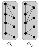
(a) Temporal graph

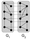
(b) Multiplex view

Figure 2: Temporal graph and its multiplex view, $m=2$.

An interesting property of the multiplex model is that temporal cuts in $\mathcal{G}$ become standard—single graph—cuts in $\chi(\mathcal{G})$. We can evaluate the sparsity of a cut in $\mathcal{G}$ by applying the original formulation (Expression 2) to $\chi(\mathcal{G})$, since both edges cut and partition changes in $\mathcal{G}$ become edges cut in $\chi(\mathcal{G})$. As an example, we show the multiplex view of cut II (Figure 3b) in Figure 3c. However, notice that not every standard cut in $\chi(\mathcal{G})$ is a valid temporal cut. For instance, cutting all the temporal edges (i.e. separating the two snapshots in our example) would be allowed in the standard formulation, but would lead to an undefined value of sparsity as the denominator in Expression 3 will be 0. Therefore, we cannot directly apply existing sparsest cut algorithms to $\chi(\mathcal{G})$ and expect to achieve a sparse temporal cut for $\mathcal{G}$.

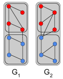
(a) Temporal cut I

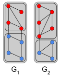
(b) Temporal cut II

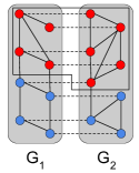
(c) Multiplex cut II

Figure 3: Two temporal graph cuts (I and II) for the graph shown in Figure 2a and multiplex view of cut II. For $\beta=1$, cut I has a sparsity ratio $\sigma$ of $(2+3+0)/(4\times 4+4\times 4)=0.16$ while cut II has a ratio of $(2+1+1)/(4\times 4+5\times 3)=0.13$. Thus, II is a sparser temporal cut.

2.1.2 Normalized Cut

A practical limitation of the cut sparsity (Equation 2), is that it favors sparsity over partition size balance. In community detection, this often leads to the discovery of “whisker communities” [23]. Normalized cuts [27] take into account the volume (i.e. sum of the degrees of vertices) of the resulting partitions, which is less prone to this effect. The normalized version of the cut sparsity is defined as:

$$\phi(X)=\frac{|(X,\overline{X})|}{vol(X).vol(\overline{X})}$$ (4)

where $vol(Y)=\sum_{v\in Y}deg(v)$ and $deg(v)$ is the degree of $v$.

Normalized cuts are related, by a constant factor, to the graph conductance [9]. We also generalize the normalized cut sparsity $\phi$ to temporal graphs as follows:

$$\phi(X_{1},\ldots X_{m};\beta)=\frac{\sum_{t=1}^{m}|(X_{t},\overline{X}_{t})|+\sum_{t=1}^{m-1}\Delta(X_{t},\overline{X}_{t+1})}{\sum_{t=1}^{m}vol(\overline{X}_{t})vol(X_{t})}$$ (5)

Next, we define the normalized cut problem for temporal graphs.

Definition 2

Normalized temporal cut. The normalized temporal cut of $\mathcal{G}$, for a constant $\beta$, is defined as:

$$\smash{\arg\min}_{X_{1}\ldots X_{m}}\phi(X_{1},\ldots X_{m};\beta)$$

Computing optimal normalized temporal cuts is NP-hard, since the problem becomes equivalent to the standard definition, also NP-hard, for the case of a single snapshot. In the next section, we discuss spectral approaches for sparsest and normalized cuts in temporal graphs.

2.2 Spectral Approaches

Similar to the single graph case, we also exploit spectral graph theory in order to compute good temporal graph cuts. Let $A$ be an $n\times n$ weighted adjacency matrix of a graph $G(V,E)$, where $A_{u,v}=W(u,v)$ if $(u,v)\in E$ or $0$, otherwise. The degree matrix $D$ is a an $n\times n$ diagonal matrix, with $D_{v,v}=deg(v)$ and $D_{u,v}=0$ for $u\neq v$. The Laplacian matrix of $G$ is defined as $L=D-A$. Let $L_{t}$ be the Laplacian matrix of the graph snapshot $G_{t}$ and $I$ be an $n\times n$ identity matrix. We define the Laplacian of the temporal graph $\mathcal{G}$ as the Laplacian of its multiplex view $\chi(\mathcal{G})$:

$$\mathcal{L}=\begin{pmatrix}L_{1}+\beta I&-\beta I&0&\ldots&0\\ -\beta I&L_{2}+2\beta I&-\beta I&\ldots&0\\ \vdots&&\ddots&\ldots&-\beta I\\ 0&0&\ldots&-\beta I&L_{m}+\beta I\end{pmatrix}$$

The matrix $\mathcal{L}$ can be also written using the Kronecker (or tensor) product as $\textbf{diag}(L_{1},\ldots L_{m})+L^{I}\otimes I$, where $L^{I}$ is the Laplacian of a line graph and $I$ is an $n\times n$ identity matrix. Similarly, we define the degree matrix $\mathcal{D}$ of $\mathcal{G}$ as $\textbf{diag}(D_{1},$ $D_{2}\ldots D_{m})$, where $D_{t}$ is the degree matrix of $G_{t}$. Let $C=nI-\textbf{1}_{n\times n}$ be the Laplacian of a complete graph with $n$ vertices, we use $C$ to define another $nm\times nm$ Laplacian matrix $\mathcal{C}=I\otimes C$ associated with $\mathcal{G}$. The matrix $\mathcal{C}$ is the Laplacian of a graph composed of $m$ isolated components of size $n$, each of them being a clique. This special matrix will be applied to enforce valid temporal cuts over the snapshots of $\mathcal{G}$. Further, we define a size-$nm$ indicator vector x. Each vertex $v\in V$ is represented $m$ times in x, one for each snapshot. The value $\textbf{x}[v_{t}]=1$ if $v_{t}\in X_{t}$ and $\textbf{x}[v_{t}]=-1$ if $v_{t}\in\overline{X}_{t}$. In the next sections, we show how to apply this spectral formulation to solve temporal cut problems.

2.2.1 Sparsest Cut

The next lemma shows how the matrices $\mathcal{L}$ and $\mathcal{C}$ can be applied to compute the sparsity of a temporal cut in $\mathcal{G}$.

Lemma 1

The sparsity of a temporal cut $\langle(X_{1},\overline{X}_{1}),$ $\ldots$ $(X_{m},\overline{X}_{m})\rangle$ can be computed as $\frac{\textbf{x}^{\intercal}\mathcal{L}\textbf{x}}{\textbf{x}^{\intercal}\mathcal{C}\textbf{x}}$.

Please refer to the extended version of this paper [30] for proofs of all Lemmas and Theorems. Based on Lemma 1, we can obtain a relaxed solution, $\textbf{x}\in[-1,1]^{nm}$, for the sparsest temporal cut problem (Definition 1) in polynomial-time using an eigenvalue computation algorithm. This solution is later rounded to adhere to the original (discrete) constraint $\textbf{x}\in\{-1,1\}^{nm}$. We make use of Lemma 6 in order to avoid expensive computations involving the matrix $\mathcal{C}$.

Lemma 2

The following property holds for the square-root pseudo-inverse $(\mathcal{C}^{+})^{\frac{1}{2}}$ of the matrix $\mathcal{C}$:

$$(\mathcal{C}^{+})^{\frac{1}{2}}=\frac{1}{\sqrt{n}}\mathcal{C}$$ (6)

The following Lemma can be applied in the computation of a relaxed solution for the sparsest temporal cut problem.

Lemma 3

A relaxed solution for sparsest temporal cut problem can be computed as:

$$\textbf{y*}=\operatorname*{arg\,min}_{\textbf{y}\in[-1,1]^{nm},\textbf{y}\perp span\{\textbf{e}_{1},\ldots\textbf{e}_{m}\}}\frac{\textbf{y}^{\intercal}\mathcal{CLC}\textbf{y}}{\textbf{y}^{\intercal}\textbf{y}}$$ (7)

$$\text{where }\textbf{e}_{i}.\lambda_{i}=\textbf{e}_{i}.\mathcal{CLC},\lambda_{1}\leq\lambda_{2}\leq\ldots\lambda_{nm}$$

The ($m$$+$$1$)-th eigenvector of the matrix $(\mathcal{CLC})$ associated with the temporal graph $\mathcal{G}$ provides a relaxed solution for the sparsest temporal cut problem. The matrices $\mathcal{L}$ and $\mathcal{C}$ have $O(mn+\sum_{t}|E_{t}|)$ and $O(n^{2}m)$ non-zeros, respectively, and thus computing the matrix product takes $O(n\sum_{t}|E_{t}|)$ time. The resulting product has $O(n^{2}m)$ non-zeros and, as a consequence, computing its ($m$$+$$1$)-th eigenvector takes $O(n^{2}m^{2})$ time in practice, which can be prohibitive in real settings. Moreover, the aforementioned lemma does not offer much insight regarding efficient solutions for our problem, as we do not know many properties of the matrix $\mathcal{CLC}$. We will define a more intuitive solution for computing sparse temporal cuts, which makes use of the following lemma.

Lemma 4

The matrix $\mathcal{C}$ commutes with any other real symmetric $nm\times nm$ matrix.

Theorem 1

A relaxed solution for the sparsest temporal cut problem can, alternatively, be computed as:

$$\textbf{x}*=\operatorname*{arg\,max}_{\textbf{x}\in[-1,1]^{nm}}\frac{\textbf{x}^{\intercal}[(3(n+2\beta)\mathcal{C}-\mathcal{L}]\textbf{x}}{\textbf{x}^{\intercal}\textbf{x}}$$ (8)

which is the largest eigenvector of $3(n+2\beta)\mathcal{C}-\mathcal{L}$.

The matrix $3(n+2\beta)\mathcal{C}-\mathcal{L}$ is a Laplacian associated with a multiplex graph in which temporal edges have weight $w^{\prime}(v_{t},v_{t+1})$$=-\beta$ and intra-layer edges have weight $w^{\prime}(u,v)$ $=3(n+2\beta)-w(u,v)$. This leads to a reordering of the spectrum of the original Laplacian $\mathcal{L}$ where cuts containing only temporal edges have negative associated eigenvalues and sparse cuts for each Laplacian $L_{t}$ become dense cuts for a new Laplacian $[3(n+2\beta))C-L_{t}]$. In terms of complexity, computing the difference $3(n+2\beta)\mathcal{C}-\mathcal{L}$ takes $O(n^{2}m)$ time and the largest eigenvector of $[3(n+2\beta)\mathcal{C}-\mathcal{L}]$ can be calculated in $O(n^{2}m)$. The resulting complexity is a significant improvement over the $O(n^{2}m^{2})$ time taken by the previous solution if the number of snapshots is large.

2.2.2 Normalized Cut

We follow the same steps as in the previous section to compute normalized temporal cuts.

Lemma 5

The normalized sparsity of a temporal cut $\langle(X_{1},$ $\overline{X}_{1}),$ $\ldots$ $(X_{m},\overline{X}_{m})\rangle$ can be computed as $\frac{\textbf{x}^{\intercal}\mathcal{L}\textbf{x}}{\textbf{x}^{\intercal}\mathcal{D}^{\frac{1}{2}}\mathcal{C}\mathcal{D}^{\frac{1}{2}}\textbf{x}}$.

Accordingly, we also define an equivalent of Lemma 3 for the case of normalized cuts.

Lemma 6

A relaxed solution for the normalized temporal cut problem can be computed as:

$$\textbf{y*}=\operatorname*{arg\,min}_{\textbf{y}\in[-1,1]^{nm},\textbf{y}\perp span\{\textbf{e}_{1},\ldots\textbf{e}_{m}\}}\frac{\textbf{y}^{\intercal}\mathcal{C}(\mathcal{D}^{+})^{\frac{1}{2}}\mathcal{L}(\mathcal{D}^{+})^{\frac{1}{2}}\mathcal{C}\textbf{y}}{\textbf{y}^{\intercal}\textbf{y}}$$ (9)

$$\text{where }\textbf{e}_{i}.\lambda_{i}=\textbf{e}_{i}.\mathcal{C}(\mathcal{D}^{+})^{\frac{1}{2}}\mathcal{L}(\mathcal{D}^{+})^{\frac{1}{2}}\mathcal{C},\lambda_{1}\leq\lambda_{2}\leq\ldots\lambda_{nm}$$

As a consequence, we can apply Lemma 6 to compute a relaxed normalized temporal cut as the ($m+1$)-th eigenvector of the matrix $\mathcal{C}(\mathcal{D}^{+})^{\frac{1}{2}}\mathcal{L}(\mathcal{D}^{+})^{\frac{1}{2}}\mathcal{C}$. We finish by providing an equivalent of Theorem 1, for the normalized case.

Theorem 2

A relaxed solution for the sparsest temporal cut problem can, alternatively, be computed as:

$$\textbf{x}*=\operatorname*{arg\,max}_{\textbf{x}\in[-1,1]^{nm}}\frac{\textbf{x}^{\intercal}[(3(n+2\beta)\mathcal{C}-(\mathcal{D}^{+})^{\frac{1}{2}}\mathcal{L}(\mathcal{D}^{+})^{\frac{1}{2}}]\textbf{x}}{\textbf{x}^{\intercal}\textbf{x}}$$ (10)

the largest eigenvector of $3(n+2\beta)\mathcal{C}-(\mathcal{D}^{+})^{\frac{1}{2}}\mathcal{L}(\mathcal{D}^{+})^{\frac{1}{2}}$.

The interpretation of matrix $3(n+2\beta)\mathcal{C}-(\mathcal{D}^{+})^{\frac{1}{2}}\mathcal{L}(\mathcal{D}^{+})^{\frac{1}{2}}$ is similar to the one for the sparsest cut case, with temporal edges having negative weights. Moreover, the complexity of computing the largest eigenvector of such matrix is also $O(n^{2}m)$. This quadratic cost on the size of the graph, for both sparsest and normalized cut problems, becomes prohibitive even for reasonably small graphs. The next section is focused on faster algorithms for temporal graph cuts.

Algorithm 1 Spectral Algorithm

0: Temporal graph $\mathcal{G}$, rank $r$, constant $\beta$

0: Temporal cut $\langle(X_{1},\overline{X}_{1}),\ldots(X_{m},\overline{X}_{m})\rangle$

1: for $G_{t}\in\mathcal{G}$ do

2:    Compute bottom-$r$ eigendecomposition $U_{t}^{\prime}\Lambda_{t}^{\prime L}U_{t}^{\prime\intercal}\approx L_{t}$

3:    Fix $\Lambda_{t}\leftarrow\textbf{diag}(0,3(n+2\beta)n-\lambda_{n},\ldots 3(n+2\beta)n-\lambda_{2})$

4: end for

5: $\mathcal{Q}\leftarrow\textbf{diag}(\Lambda_{1},\ldots\Lambda_{m})-\mathcal{B}$

6: for $t\in[1,m-1]$ do

7:    $\mathcal{Q}_{t,t+1}\leftarrow U_{t}^{\prime\intercal}U^{\prime}_{t+1}$

8: end for

9: Compute largest eigenvector $\textbf{x*}\leftarrow\arg\max_{\textbf{x}}\textbf{x}^{\intercal}\mathcal{Q}\textbf{x}/\textbf{x}^{\intercal}\textbf{x}$

10: return rounded cut $\textbf{sweep}(\mathcal{U}.\textbf{x}*,\mathcal{G},\beta)$

2.3 Fast Approximations

By definition, sparse temporal cuts are sparse in each snapshot and smooth across snapshots. Similarly, normalized temporal cuts are composed of a sequence of good normalized snapshot cuts that are stable over time. This motivates divide-and-conquer approaches for computing temporal cuts that first find a good cut on each snapshot (divide) and then combine them (conquer). These solutions have the potential to be much more efficient than the ones based on Theorems 1 and 2 if the conquer step is fast. However, they could lead to sub-optimal results, as optimal temporal cuts might not be composed of each snapshot’s best cuts. Instead, better divide-and-conquer schemes can explore multiple snapshot cuts in the conquer step to avoid local optima. Since we are working in the spectral domain, it is natural to take eigenvectors of blocks of $\mathcal{M}_{S}=3(n+2\beta)\mathcal{C}-\mathcal{L}$ and $\mathcal{M}_{N}=3(n+2\beta)\mathcal{C}-(\mathcal{D}^{+})^{\frac{1}{2}}\mathcal{L}(\mathcal{D}^{+})^{\frac{1}{2}}$, as continuous notions of snapshot cuts. This section will describe this general divide-and-conquer approach. We will focus our discussion on the sparsest cut problem and then briefly show how it can be generalized to normalized cuts.

The following theorem is the basis of our divide-and-conquer algorithm. It relates the spectrum of $\mathcal{M}_{S}$ to the spectrum of each of its dense diagonal blocks.

Theorem 3

The eigenvalues of the matrix $\mathcal{M}_{S}=3(n+2\beta)\mathcal{C}-\mathcal{L}$ are the same as the ones for the matrix $\mathcal{Q}$:

$$\small\mathcal{Q}=\mathbf{\Lambda}-\beta\begin{pmatrix}I&-U_{1}^{\intercal}U_{2}&0&\ldots&0\\ -U_{2}^{\intercal}U_{1}&2I&-U_{2}^{\intercal}U_{3}&\ldots&0\\ \vdots&&\ddots&\ldots&U_{m-1}^{\intercal}U_{m}\\ 0&0&\ldots&U_{m}^{\intercal}U_{m-1}&I\end{pmatrix}$$

where $U_{t}\Lambda_{t}U_{t}^{\intercal}$ is the eigendecomposition of $M_{t}=(3(n+2\beta)C-L_{t})$ and $\mathbf{\Lambda}=\textbf{diag}(\Lambda_{1}\ldots\Lambda_{m})$. An eigenvector $\textbf{e}_{j}$ of $\mathcal{M}_{S}$ is computed as $\mathcal{U}.\textbf{e}_{j}^{\mathcal{Q}}$, where $\mathcal{U}=\textbf{diag}(U_{1}\ldots$ $U_{m})$ and $\textbf{e}_{j}^{\mathcal{Q}}$ is the corresponding eigenvector of $\mathcal{Q}$.

The matrix $\mathcal{Q}$ has $O(n^{2}m)$ non-zeros, being asymptotically as sparse as $\mathcal{M}_{S}$. However, $\mathcal{Q}$ can be block-wise sparsified using low-rank approximations of the matrices $M_{t}$. Given a constant $r\leq n$, we approximate each $M_{t}$ as $U_{t}\Lambda_{t}^{\prime}U_{t}^{\intercal}$, where $\Lambda_{i}^{\prime}$ contains only the top-$r$ eigenvalues of $M_{t}$. The benefits of such a strategy are the following: (1) The cost of computing the eigendecomposition of $M_{t}$ changes from $O(n^{3})$ to $O(rn^{2})$; (2) the cost of multiplying eigenvector matrices decreases from $O(n^{3})$ to $O(r^{3})$; and (3) the number of non-zeros in $\mathcal{Q}$ is reduced from $O(n^{2}m)$ to $O(r^{2}m)$. Similar to the case of general block tridiagonal matrices [13], we can show that the error associated with such approximation is bounded by $2\lambda_{r+1}^{max}$, where $\lambda_{r+1}^{max}$ is the largest $(r+1)$-nth eigenvalue of the approximated matrices $M_{t}$.

We improve our approach even further by speeding-up the eigendecomposition of the matrices $M_{t}$ without any additional error. The idea is to operate directly over the original Laplacians $L_{t}$, which are expected to be sparse. The eigendecomposition of a sparse matrix with $|E|$ edges can be performed in time $O(n|E|)$ and for real-world graphs $|E|<<n^{2}$. The following Lemma shows how the spectrum of $M_{t}$ can be efficiently computed based on $L_{t}$.

Lemma 7

Let $\lambda_{1}^{L},\lambda_{2}^{L}\ldots\lambda_{n}^{L}$ be the eigenvalues of a (connected) Laplacian matrix $L$ in increasing order with associated eigenvectors $e_{1}^{L},e_{2}^{L}\ldots e_{n}^{L}$. The eigenvectors $e_{i}^{L}$ are also eigenvectors of $3(n+2\beta)C-L$ with associated eigenvalues $\lambda_{1}=0$ and $\lambda_{i}=3(n+2\beta)n-\lambda_{n-i+1}$ for $i>0$.

Algorithm 1 describes our divide-and-conquer approach for approximating the sparsest temporal graph cut. Its inputs are the temporal graph $\mathcal{G}$, the rank $r$ that controls the accuracy of the algorithm, and a constant $\beta$. As a result, it returns a cut $\langle(X_{1},\overline{X}_{1})\ldots$ $(X_{m},\overline{X}_{m})\rangle$ that (approximately) minimizes the sparsity ratio defined in Equation 3. In the divide phase, the top-$r$ eigenvalues/eigenvectors of each matrix $M_{t}$—related to the bottom-$r$ eigenvalues/eigenvectors of $L_{t}$—are computed using Lemma 7 (steps 1-5). The conquer phase (steps 6-11) consists of building the matrix $\mathcal{Q}$, as described in Theorem 3, and then computing its largest eigenvector as a relaxed version of a sparse temporal cut. The resulting eigenvector is discretized using a standard sweep algorithm (sweep) over the vertices sorted by their corresponding value of x*. The selection criteria for the sweep algorithm is the sparsity ratio given by Equation 3.

The time complexity of our algorithm is $O(mr\sum_{t=1}^{m}|E_{t}|$ $+mr^{3})$. The divide step has cost $O(mr\sum_{t=1}^{m}|E_{t}|)$, which corresponds to the computation of $r$ eigenvectors/eigenvalues of Laplacian matrices $L_{t}$ with $O(|E_{t}|)$ non-zeros each. As each snapshot is processed independently, this part of the algorithm can be easily parallelized. In the conquer step, the most time consuming operation is in computing $m-1$ $r\times r$ matrix products in the construction of $\mathcal{Q}$, which takes $O(r^{3}m)$ time in total. Moreover, our algorithm has space complexity of $O(r^{2}m)$. This is due to the number of non-zeros in the sparse representation of $\mathcal{Q}$, which is, asymptotically, the largest data structure applied in the computation.

We follow the same general approach discussed in this section to efficiently compute normalized temporal cuts. As in Theorem 3, we can compute the eigenvectors of $\mathcal{M}_{N}$ using divide-and-conquer. However, each block $M_{t}$ will be in the form $3(n-2\beta)C-(D_{t}^{+})^{\frac{1}{2}}L_{t}(D_{t}^{+})^{\frac{1}{2}}$. Moreover, similar to Lemma 7, we can also compute the eigendecomposition of $M_{t}$ based on $(D_{t}^{+})^{\frac{1}{2}}L_{t}(D_{t}^{+})^{\frac{1}{2}}$.

2.4 Generalizations

Here, we briefly address several generalizations of temporal cuts that aim to increase the applicability of this work.

Arbitrary swap costs: While we have assumed uniform swap costs $\beta$, generalizing our formulation to arbitrary (non-negative) swap costs for pairs $(v_{t},v_{t+1})$ is straightforward.

Multiple cuts: Multi-cuts can be computed based on the top eigenvectors of our temporal cut matrices, as proposed in [27]. Eigenvector values are given to a clustering algorithm (e.g. k-means) to obtain a $k$-way partition.

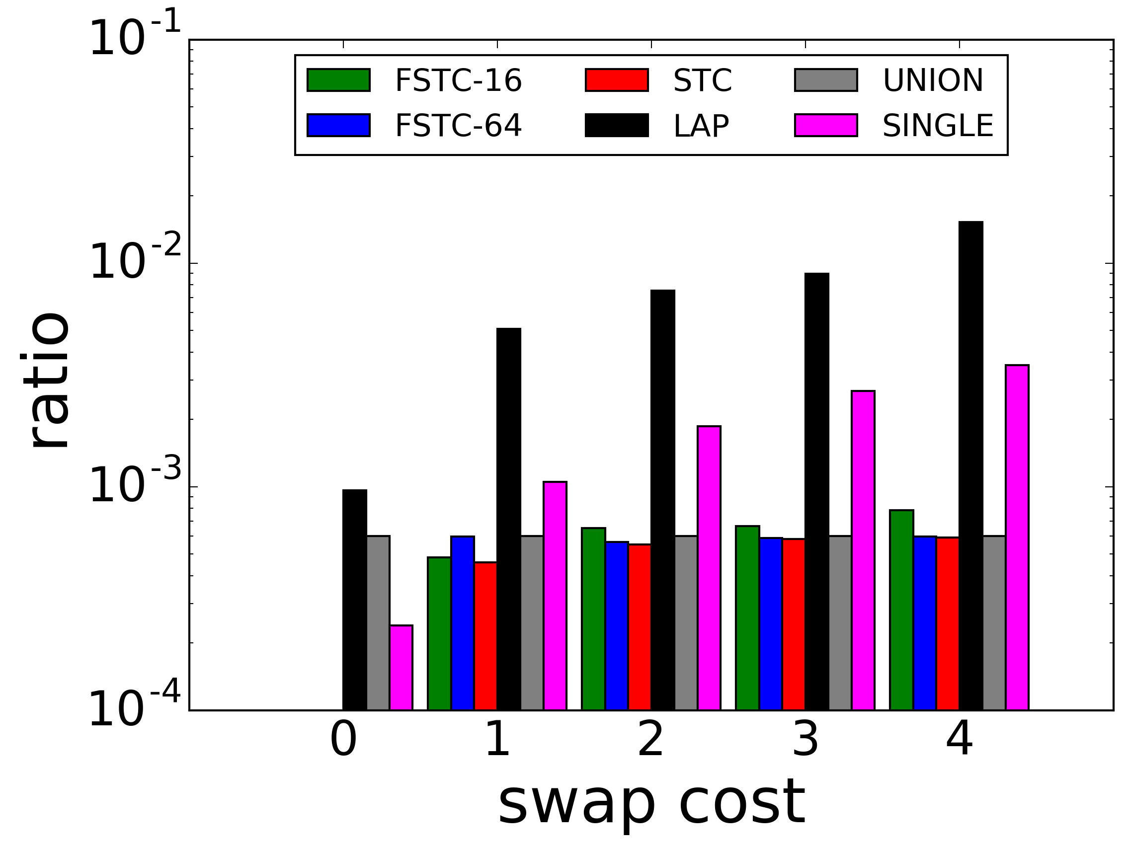
(a) Synthetic

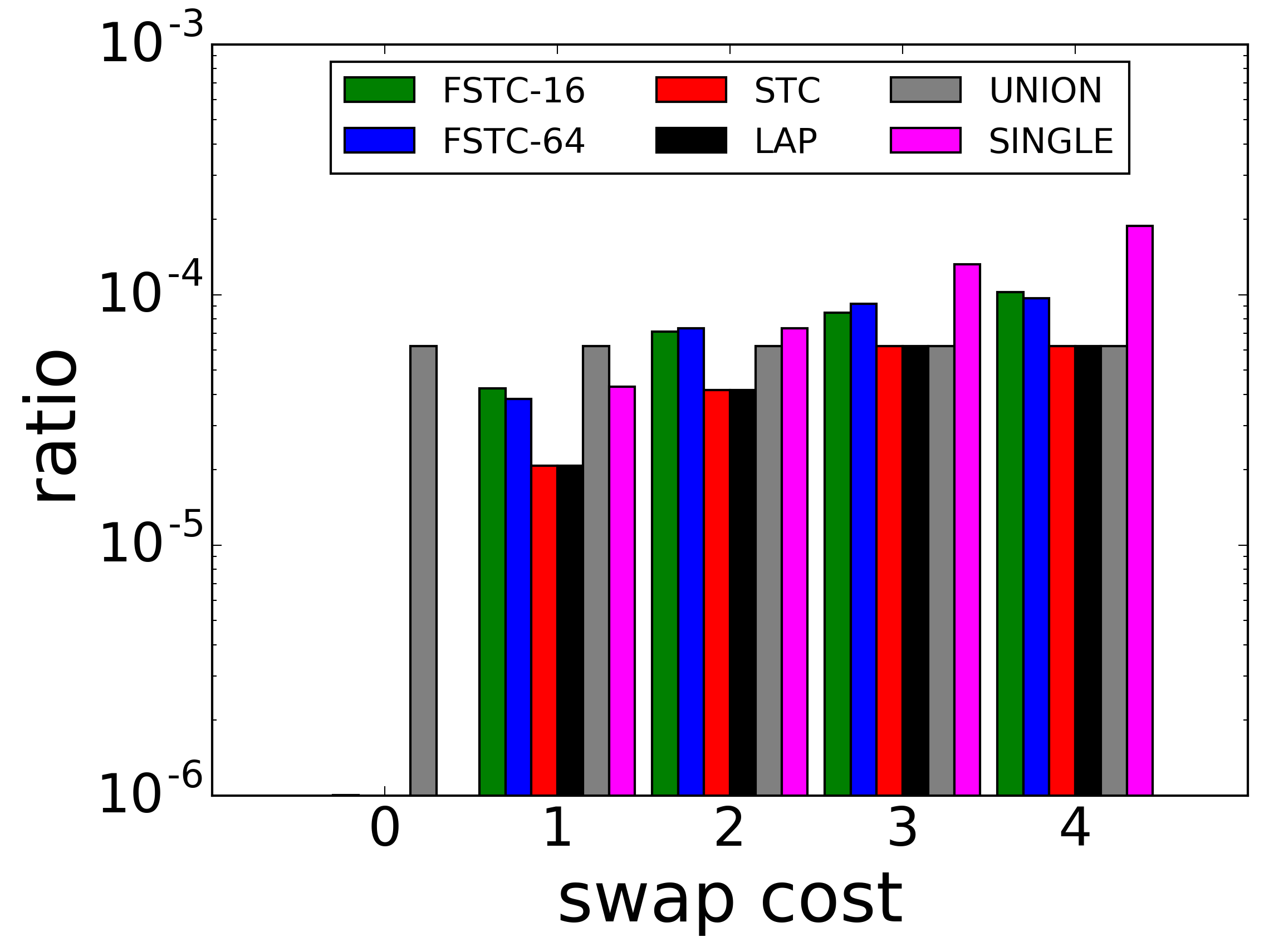
(b) School

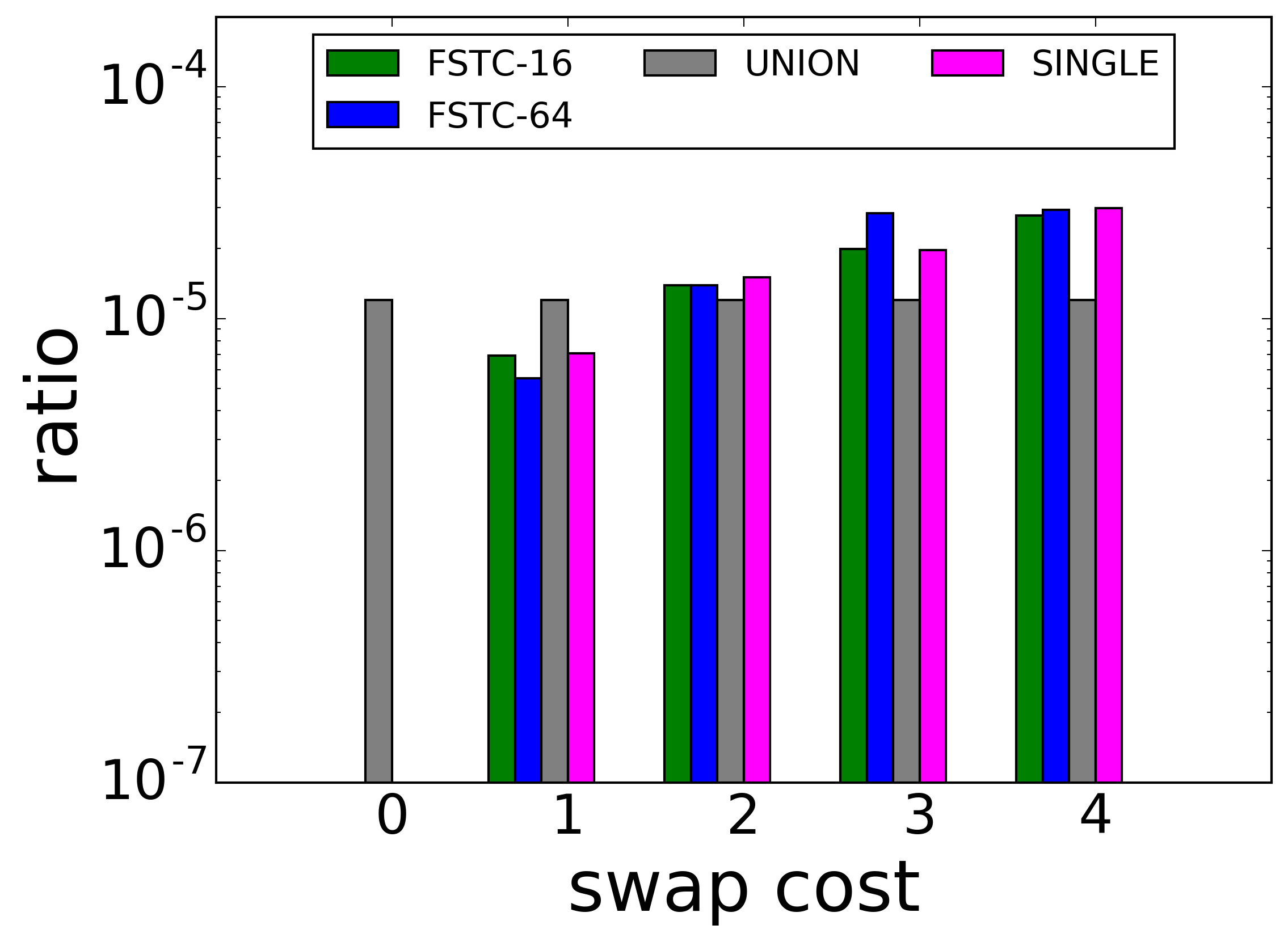
(c) Stock

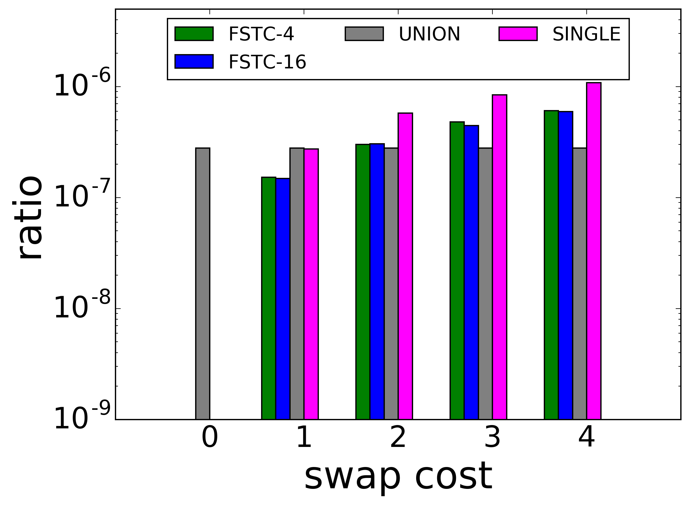
(d) DBLP

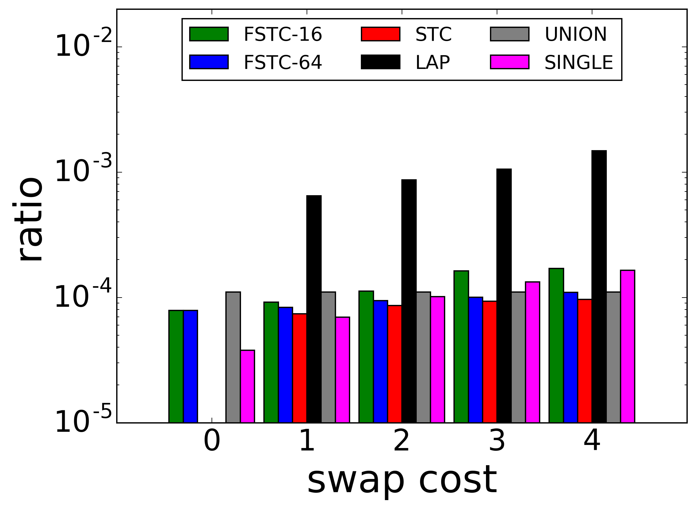
(e) Synthetic

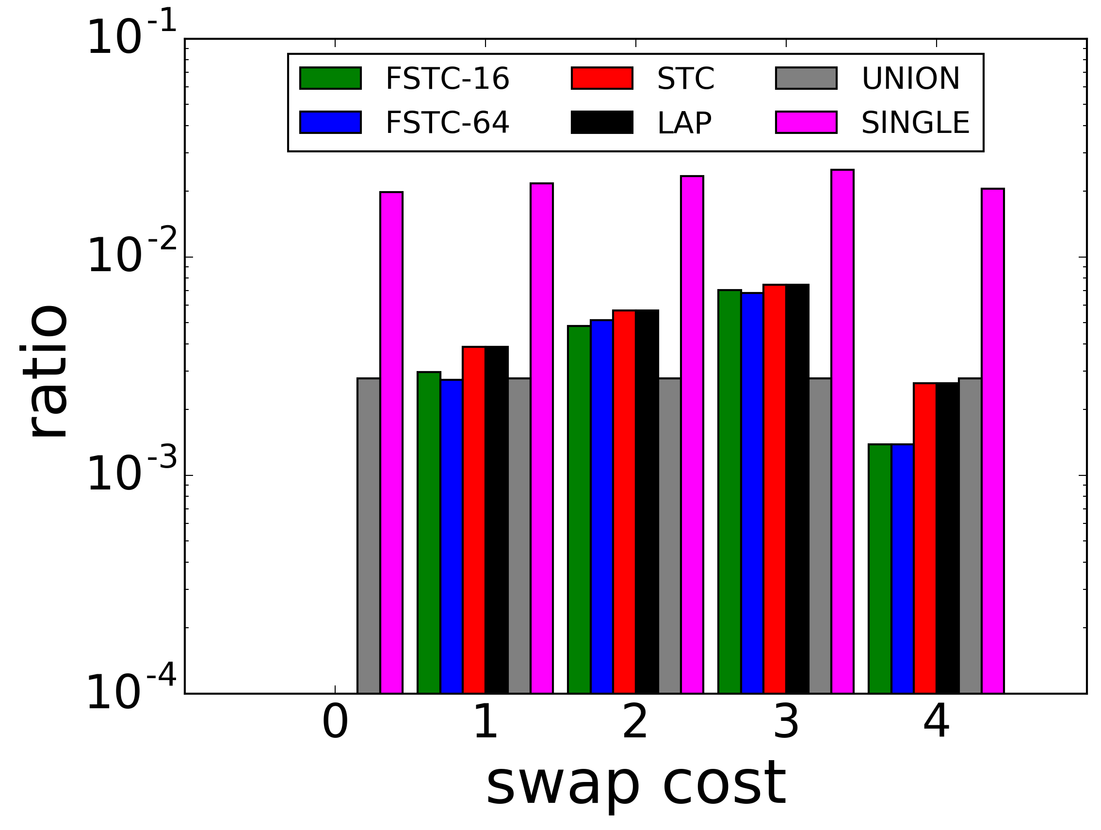
(f) School

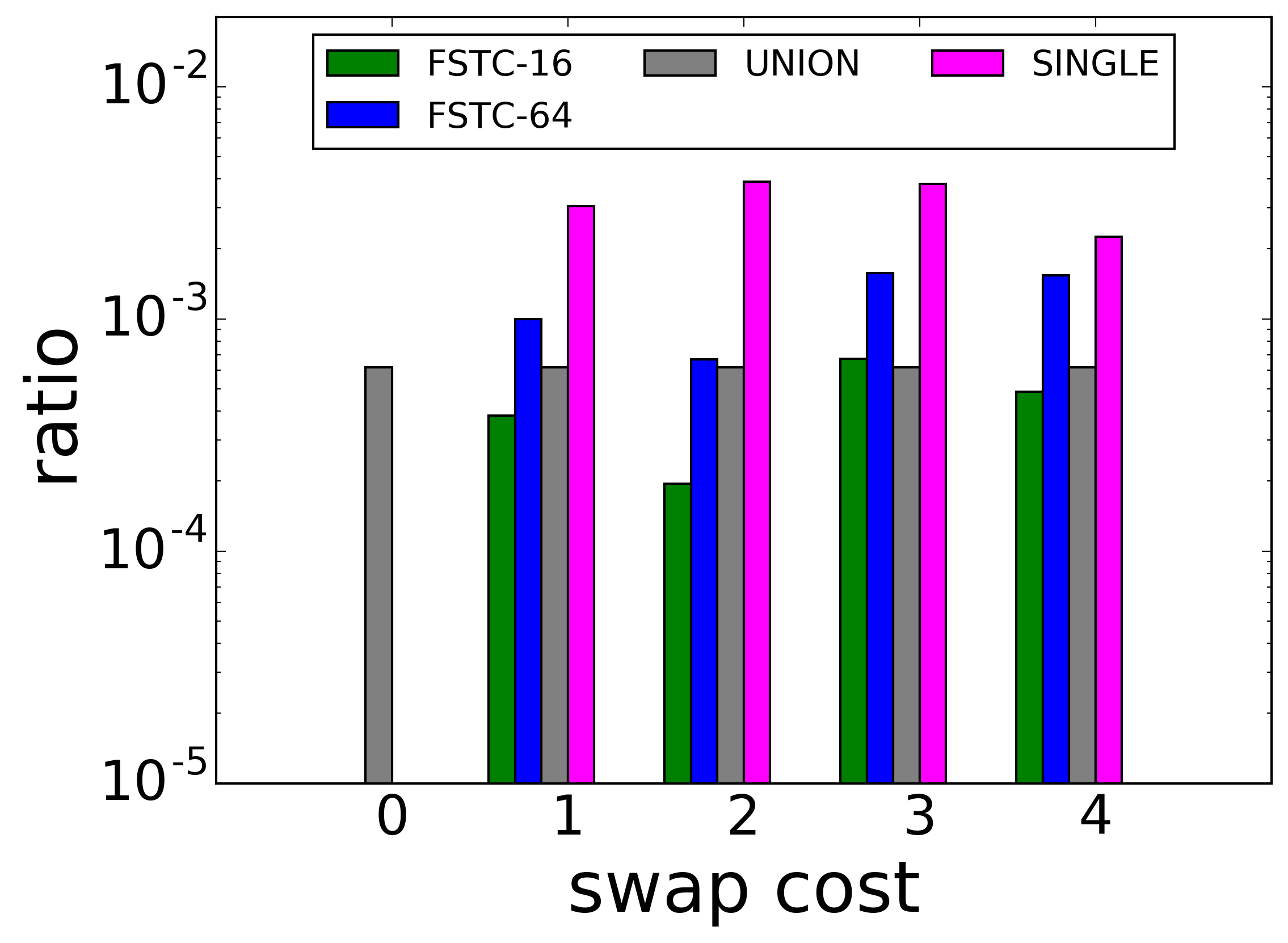
(g) Stock

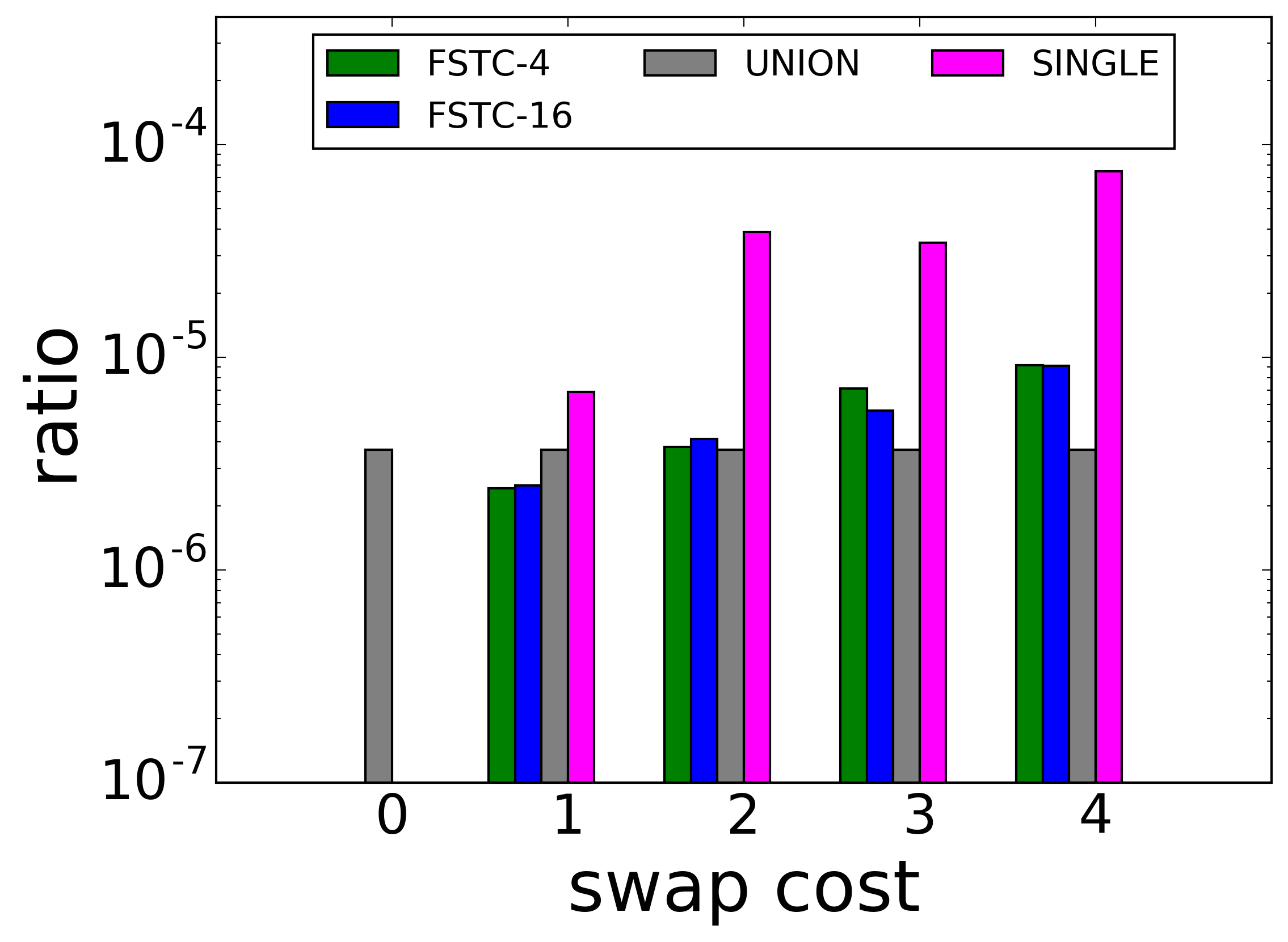
(h) DBLP

Figure 4: Quality results (sparsity ratios) for sparsest (a-d) and normalized (e-h) cuts on synthetic and real datasets.

3 Signal Processing on Graphs

We apply graph cuts as data-driven wavelet bases for dynamic signals. The idea is to identify temporal cuts based on both graph structure and signal to compute wavelet coefficients using the resulting partitions. Given a sequence of signals $\langle\textbf{f}_{(1)},\ldots\textbf{f}_{(m)}\rangle$, $\textbf{f}_{(i)}\in\mathbb{R}^{n}$, on a temporal graph $\mathcal{G}$, our goal is to discover a temporal cut that is sparse, smooth, and separates vertices with dissimilar signal values. A previous work [29] has shown that a relaxation of the $L_{2}$ energy (or importance) $||a||_{2}$ of a wavelet coefficient $a$ for a single graph snapshot with signal f can be computed as:

$$\frac{(|X|\sum_{v\in\overline{X}}\textbf{f}[v]-|\overline{X}|\sum_{u\in X}\textbf{f}[u])^{2}}{|X||\overline{X}|}\propto-\frac{\textbf{x}^{\intercal}CSC\textbf{x}}{\textbf{x}^{\intercal}C\textbf{x}}$$ (11)

where x is an indicator vector and $S_{u,v}=(\textbf{f}[v]-\textbf{f}[u])^{2}$. Sparsity is enforced by adding a Laplacian regularization factor $\alpha\textbf{x}^{\intercal}L\textbf{x}$, where $\alpha$ is a user-defined constant, to the denominator of Equation 11. This formulation supports an algorithm for computing graph wavelets, which we extend to dynamic signals. Following the same approach as in Section 2.1, we apply the multiplex graph representation to compute the energy of a dynamic wavelet coefficient:

$$\frac{\sum_{t=1}^{m}\Theta_{t}^{2}+\sum_{t=1}^{m-1}\Theta_{t}\Theta_{t+1}}{\sum_{t=1}^{m}|X_{t}||\overline{X}_{t}|}$$ (12)

where $\Theta_{t}=|X_{t}|\sum_{v\in\overline{X}_{t}}\textbf{f}[v]-|\overline{X}_{t}|\sum_{u\in X_{t}}\textbf{f}[u]$. The first term in the numerator of Equation 12 is the sum of the numerator of Equation 11 over all snapshots. The second term acts on sequential snapshots and enforces the partitions to be consistent over time —i.e. $X_{t}$’s to be jointly associated with either large or small values. Intuitively, the energy is maximized for partitions that separate different values and are also balanced in size. The next theorem provides a spectral formulation for the energy of dynamic wavelets.

Theorem 4

The energy of a dynamic wavelet is proportional to $-\frac{\textbf{x}^{\intercal}\mathcal{C}\mathcal{S}\mathcal{C}\textbf{x}}{\textbf{x}^{\intercal}\mathcal{C}\textbf{x}}$, where $\mathcal{S}_{u,v}=(\textbf{f}[u]-\textbf{f}[v])^{2}$ for values within one snapshot from each other.

We apply Theorem 4 to compute a relaxation of the optimal dynamic wavelet as a regularized eigenvalue problem:

$$\textbf{x}*=\smash{\operatorname*{arg\,min}_{\textbf{x}\in[-1,1]^{nm}}}\frac{\textbf{x}^{\intercal}\mathcal{CSC}\textbf{x}}{\textbf{x}^{\intercal}\mathcal{C}\textbf{x}+\alpha\textbf{x}^{\intercal}\mathcal{L}\textbf{x}}$$ (13)

where $\mathcal{C}$ and $\mathcal{L}$ are the matrices defined in Section 2.1. The same optimizations discussed in [29] can also be applied to efficiently approximate Equation 13. The resulting algorithm has complexity $O(pn\sum_{t}|E_{t}|+qn^{2}m^{2})$, where $p$ and $q$ are small constants. Similar to Algorithm 1, we apply a sweep procedure to obtain a cut from vector $\textbf{x}*$.

4 Experiments

4.1 Datasets

School is a contact network where vertices represent children from a primary school and edges are created based on proximity detected by sensors [34], with $242$ vertices, $17K$ edges and $3$ snapshots. Edge weights are based on the duration of the contact within an interval. Stock is a correlation network of US stocks’ end of the day prices, where stocks are connected if their absolute correlation is at least $.05$ and edge weights are the absolute correlation values. The resulting network has $500$ vertices, $27K$ edges, and $26$ snapshots (one for each year in the interval 1999-2015). DBLP is a sample from the DBLP collaboration network. Vertices corresponding to two authors are connected in a given snapshot if they co-authored a paper in the corresponding year. We selected authors who published at least 5 papers one of the following conferences: KDD (data mining), CVPR (computer vision), and FOCS (theory). The resulting temporal network has $3.4K$ vertices, $16.4K$ edges, and $4$ snapshots.

We also use a synthetic data generator. Its parameters are a graph size $n$, partition size $k<n$, number of hops $h$, and noise level $0\leq\epsilon\leq 1$. Edges are created based on a $\lceil\sqrt{n}\rceil\times\lceil\sqrt{n}\rceil$ grid, where each vertex is connected to its $h$-hop neighbors. A partition is a sub-grid initialized with $\lceil\sqrt{k}\rceil\times\lceil\sqrt{k}\rceil$ dimensions ($k=n/2$). A value $\pi(v)=1.+N(0,\epsilon)$ is assigned to vertices inside the partition and the remaining vertices receive iid realizations of a Gaussian $N(0,\epsilon)$. Given the node values, the weight $w$ of an edge $(u,v)$ is set as $\exp{(|\pi(v)-\pi(u)|)}$. To produce the dynamics, we move the partition along the main diagonal of the grid.

To evaluate our wavelets for dynamic signals, we apply our approach to Traffic [29], a road network from California with $100$ vertices, $200$ edges, and $12$ snapshots. Average vehicle speeds measured at the vertices of the network were taken as a dynamic signal for the timespan of a Friday in April, 2011. Moreover, we apply the heat equation to generate synthetic signals over the School network. Different from Traffic, which has a static structure, the resulting dataset (School-heat) is dynamic in structure and signal.

4.2 Approximation and Performance

Two general approaches for computing temporal cuts, for both sparsest and normalized cuts, are evaluated in this section. The first approach, STC, is based on Theorems 1 and 2, for sparsest and normalized cuts, respectively. The second approach, FSTC-r, for a rank $r$, applies the fast approximation described in Section 2.3.

We consider three baselines in this evaluation. SINGLE is a heuristic that first discovers the best cut on each snapshot and then combines them into a temporal cut. UNION computes the best average cut over all the snapshots—a cut over the union of the snapshots. LAP is similar to our approach, but operates directly on the Laplacian matrix $\mathcal{L}$. Notice that each of these baselines can be applied to either sparsest and normalized cuts as long as the appropriate (standard or normalized) Laplacian matrix is used.

Figure 4 shows the quality results (sparsity ratios) of the methods using real and synthetic data. We vary the swap cost ($\beta$) within a range that enforces local and global (or stable) patterns. The values of $\beta$ shown are normalized to integers for ease of comparison. STC and LAP took too long to finish for the Stock and DBLP datasets, and thus such results are omitted. STC achieves the best results (smallest ratios) in most of the settings. For the School dataset, LAP also achieves good results, which is due to the small number of snapshots in the network, which makes sparse cuts in $\mathcal{L}$ coincide with good temporal cuts. UNION performs well for Stock and DBLP with large swap costs, as these settings enforce a fixed cut over time. SINGLE achieves good results only when swap costs are close to $0$, when the smoothness of the cuts do not affect the sparsity ratio. Our fast approximation (FSTC) achieves good results in most of the settings, specially for $r=64$, being able to adapt to different swap costs. Running time results (see Appendix) show that FSTC significantly outperforms STC and is competitive with SINGLE and UNION.

k	Method	Cut	Sparsity	N-sparsity	Modularity
2	GenLovain	2.6	1.0e-4	5.0e-3	102.0
	Facetnet	6.0	3.8e-4	.012	95.7
	Sparsest	2.6	1.0e-4	5.0e-3	102.0
	Norm.	2.6	1.0e-4	5.0e-3	102.0
5	GenLovain	8.0	6.8e-4	2.7e-2	110.0
	Facetnet	10.0	8.4e-4	3.0e-2	106.0
	Sparsest	8.3	6.4e-4	2.6e-2	109.0
	Norm.	6.1	9.9e-4	1.8e-2	110.0

(a) School

k	Method	Cut	Sparsity	N-sparsity	Modularity
2	GenLovain	80.	3.9e-4	1.3e-5	38,612
	Facetnet	267.0	2.6e-3	8.9e-5	33,091
	Sparsest	9.0	7.6e-5	3.6e-6	38,450
	Norm.	19.0	1.2e-4	3.8e-6	38,516
5	GenLovain	174.	1.3e-3	4.1e-5	39,342
	Facetnet	501.0	7.2e-3	2.8e-4	30,116
	Sparsest	40.0	5.2e-4	6.2e-5	38,498
	Norm.	31.0	4.0e-4	1.0e-5	39,015

(b) DBLP

Table 1: Community detection results for Sparsest and Normalized Cuts (and two baselines) using School and DBLP datasets. Our methods achieve the best results for most of the metrics and are competitive in terms of modularity.

(a) I

(b) II

(c) III

(d) IV

(e) I

(f) II

(g) III

(h) IV

Figure 5: Dynamic communities discovered using sparsest (a-d) and normalized (e-h) cuts for the DBLP dataset (4 snapshots). Better seen in color.

4.3 Community Detection

As discussed in Section 1, dynamic community detection is an interesting application for temporal cuts. Two approaches from the literature, FacetNet [24] and GenLovain [4], are the baselines. We focus our evaluation on School and DBLP, which have most meaningful communities. The following metrics are considered for comparison:

Cut: Total weight of the edges across partitions computed as $\sum_{t=1}^{m}\sum_{v,u\in G_{t}}w(u,v)(1-\delta(c_{v},c_{u}))$, where $c_{v}$ and $c_{u}$ are the partitions to which $v$ and $u$ are assigned, respectively.

Sparsity: Sparsity ratio (Equation 3) for $k$-cuts [27]:

$$\sum_{i=1}^{k}\frac{\sum_{t=1}^{m}|(X_{i,t},\overline{X}_{i,t}|+\beta\sum_{t=1}^{m-1}|(X_{i,t},\overline{X}_{i,t+1})|}{\sum_{t=1}^{m}|X_{i,t}||\overline{X}_{i,t}|}$$

N-sparsity: Normalized $k$-cut ratio (similar to sparsity).

Modularity: Temporal modularity, as defined in [4].

The baselines parameters were varied within a reasonable range of values and the best results were chosen. For GenLovain, we fixed the number of partitions by agglomerating pairs while maximizing modularity [4] and for FacetNet, we assign each vertex to its highest weight partition.

(a) I

(b) II

(c) III

(d) IV

(e) I

(f) II

(g) III

(h) IV

(i) I

(j) II

(k) III

(l) IV

Figure 6: Wavelet cut of a 4-snapshot dynamic traffic network with vehicle speeds as a signal. Vertex colors correspond to speed values (red for high and blue for low) and shapes indicate the partitions for 3 different settings: $\alpha=0.$ and $\beta=1$ (a-d, no network effect), $\alpha=200.$ and $\beta=1.$ (e-h, large network effect with low smoothness), and $\alpha=200.$ and $\beta=10.$ (i-l, large network effect and high smoothness) .

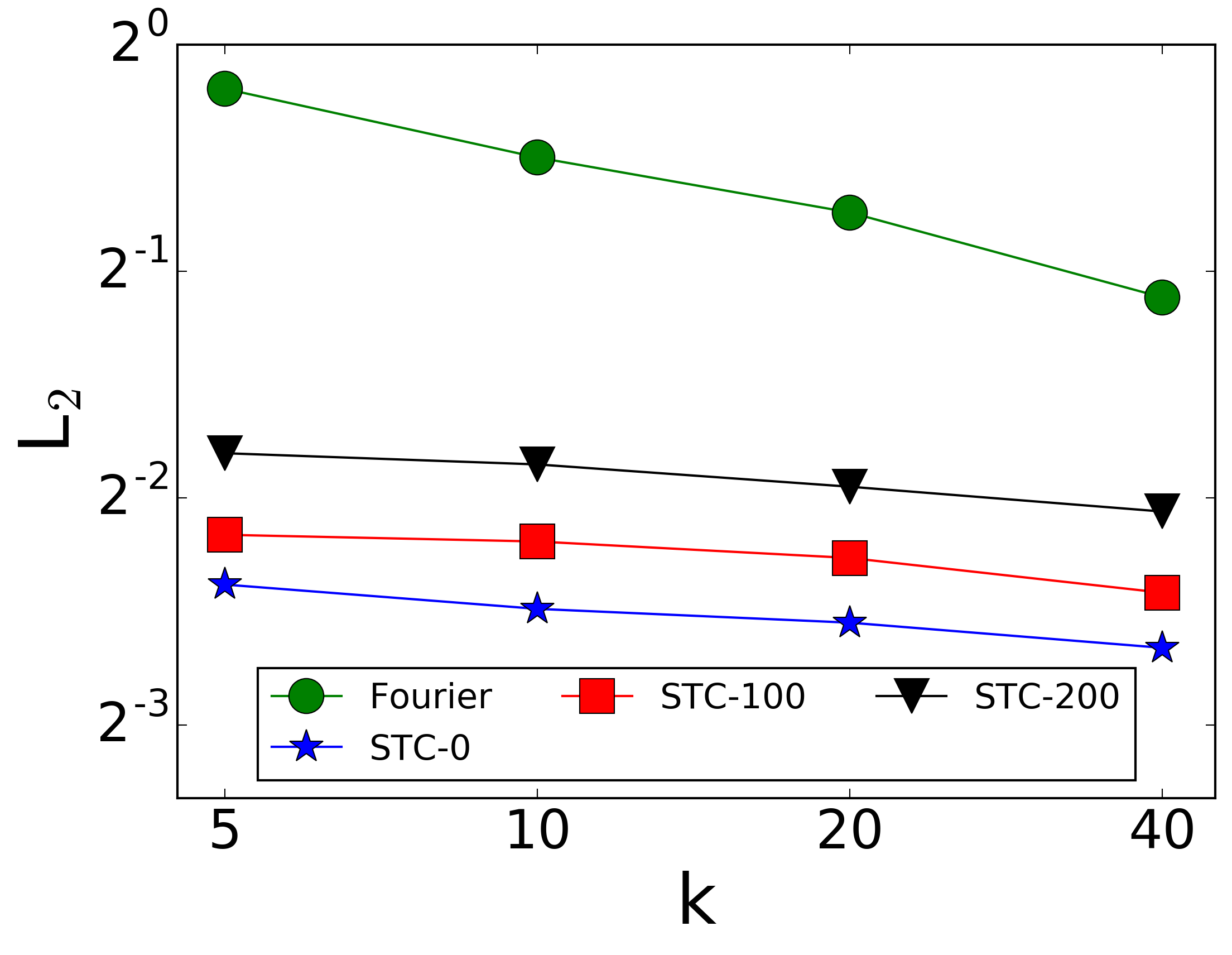
(a) Traffic

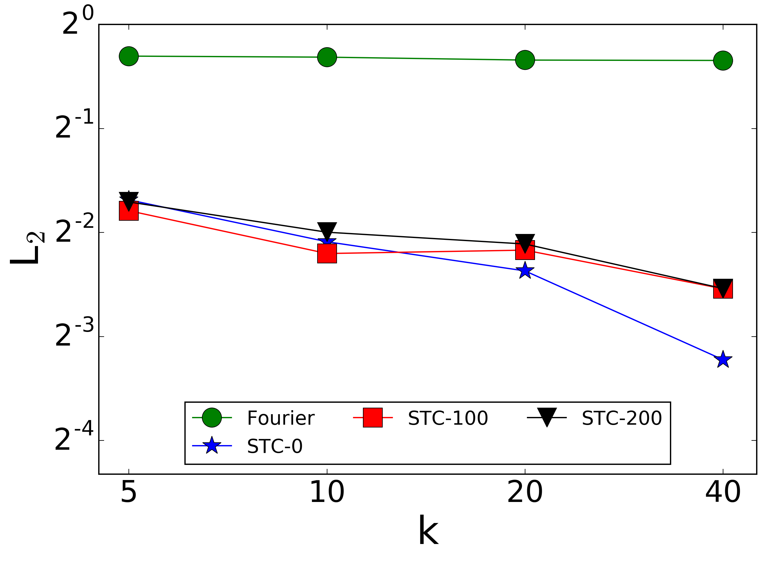
(b) School-heat

Figure 7: $L_{2}$ error with different representation sizes $k$ for Graph Fourier and our approach while setting the regularization parameter $\alpha$ to $200$, $100$, and $0$.

Community detection results, for $2$ and $5$ communities, are shown in Table 1. For School (1a), both GenLovain and our methods found the same communities ($\beta=0.25$) when $k=2$, outperforming FacetNet in all the metrics. However, for $k=5$, different communities were discovered by the methods, with Sparsest and Normalized Cuts achieving the best results in terms of sparsity and n-sparsity, respectively. Our methods also achieve competitive results in terms of modularity. Similar results were found using DBLP ($\beta=0.5$), as shown in Table 1b, although Sparsest and Normalized Cuts switch as the best method for each other’s metric in some settings. This is possible because our algorithms are approximations (i.e. not optimal). We illustrate the communities found in School ($k=2$, same as single cut) and DBLP ($k=5$) in Figures 1 and 5, respectively.

4.4 Signal Processing on Graphs

We finish our evaluation with the analysis of dynamic signals on graphs. In Figure 6, we illustrate three dynamic wavelets for Traffic discovered using our approach under different settings. First, in Figures 6a-6d, we consider cuts that take only the graph signal into account by setting both the regularization parameter $\alpha$ and the smoothness parameter $\beta$ to $0$, which leads to a cut that follows the traffic speeds but has many edges and is not smooth. Next (Figures 6e-6h), we increase $\alpha$ to $200$, producing a much sparser cut that is still not smooth. Finally, in Figures 6i-6l, we increase the smoothness $\beta$ to $10$, which forces most of the vertices to remain in the same partition despite of speed variations.

We also evaluate our approach in signal compression, which consists of computing a compact representation for a dynamic signal. As a baseline, we consider the Graph Fourier scheme [28] applied to the temporal graph (i.e. the multiplex graph that combines all the snapshots). The size of the representation ($k$) is the number of partitions and the number of top eigenvectors for our method and Graph Fourier, respectively. Figures 7a and 7b show the compression results in terms of $L_{2}$ error using a fixed representation size $k$ for the Traffic and School-heat datasets, respectively. We vary the value of the regularization parameter $\alpha$, which controls the impact of the network structure over the wavelets computed, for our method. As expected, a larger value of $\alpha$ leads to a higher $L_{2}$ error. However, even for a high regularization, our approach is still able to compute wavelets that accurately compress the signal, outperforming the baseline.

5 Conclusion

This paper studied cut problems in temporal graphs. Extensions of two existing graph cut problems, the sparsest and normalized cuts, by enforcing the smoothness of cuts over time, were introduced. To solve these problems, we have proposed spectral approaches based on multiplex graphs that compute relaxed versions of temporal cuts as eigenvectors. Scalable versions of our solutions using divide-and-conquer and low-rank matrix approximation were also presented. In order to compute cuts that take into account also graph signals, we have extended graph wavelets to the dynamic setting. Experiments have shown that our temporal cut algorithms outperform the baseline methods in terms of quality and are competitive regarding running time. Moreover, temporal cuts enable the discovery of dynamic communities and the analysis of dynamic processes on graphs.

This work opens several lines for future investigation: (i) temporal cuts, as a general framework for solving problems involving dynamic data, can be applied in many scenarios, we are particularly interested to see how our method performs in computer vision tasks; (ii) Perturbation Theory can provide deeper theoretical insights into the properties of temporal cuts (see [35, 31]); finally, (iii) we want to study Cheeger inequalities [9] for temporal cuts, as means to better understand the performance of our algorithms.

Acknowledgment. Research was sponsored by the Army Research Laboratory and was accomplished under Cooperative Agreement Number W911NF-09-2-0053 (the ARL Network Science CTA). The views and conclusions contained in this document are those of the authors and should not be interpreted as representing the official policies, either expressed or implied, of the Army Research Laboratory or the U.S. Government. The U.S. Government is authorized to reproduce and distribute reprints for Government purposes notwithstanding any copyright notation here on.

Proof of Lemma 1

Proof .1.

Since $\mathcal{L}$ is the Laplacian of $\chi(\mathcal{G})$:

$$\begin{split}\textbf{x}^{\intercal}\mathcal{L}\textbf{x}&=\sum_{(u,v)\in\mathcal{E}}(\textbf{x}[u]-\textbf{x}[v])^{2}W(u,v)\\ &=\sum_{t=1}^{m}\sum_{(u,v)\in E_{t}}(\textbf{x}[u]-\textbf{x}[v])^{2}W(u,v)\\ &\quad+\beta\sum_{t=1}^{m-1}\sum_{v\in V}(\textbf{x}[v_{t}]-\textbf{x}[v_{t+1}])^{2}\\ &=4\sum_{t=1}^{m}|(X_{t},\overline{X}_{t})|+4\sum_{t=1}^{m-1}\Delta(X_{t},\overline{X}_{t+1})\\ \end{split}$$

Regarding the denominator:

$$\begin{split}\textbf{x}^{\intercal}\mathcal{C}\textbf{x}&=\sum_{t=1}^{m}\sum_{u\neq v}(\textbf{x}[v_{t}]-\textbf{x}[u_{t}])^{2}\\ &=4\sum_{t=1}^{m}|X_{t}||\overline{X}_{t}|\end{split}$$

Proof of Lemma 6

Proof .2.

The spectrum of $C$ is $(\textbf{e}_{1},\lambda_{1})=(\textbf{1}_{n},0)$ and $\lambda_{2}=\ldots=\lambda_{n}=n$ for any vector $\textbf{e}_{i}\perp\textbf{1}_{n}$. As a consequence, the spectrum of $\mathcal{C}$ is in the form: $\lambda_{1}=\ldots=\lambda_{m}=0$ and $\lambda_{m+1}=\ldots\lambda_{nm}=n$ for any vector $\textbf{e}_{i}\perp\textbf{span}\{e_{1},\ldots e_{m}\}$. We factorize $\mathcal{C}$ as $U\Lambda U^{\intercal}=n\sum_{t=m+1}^{mn}\textbf{e}_{i}.\textbf{e}_{i}^{\intercal}$, where $U$ and $\Lambda$ are eigenvector and eigenvalue matrices of $\mathcal{C}$. Similarly, we can factorize $\mathcal{C}^{+}=\frac{1}{n}\sum_{t=m+1}^{mn}\textbf{e}_{i}.\textbf{e}_{i}^{\intercal}=\frac{1}{n^{2}}\mathcal{C}$. Taking the square-root, $(\mathcal{C}^{+})^{\frac{1}{2}}=\frac{1}{n}\mathcal{C}^{\frac{1}{2}}=\frac{1}{\sqrt{n}}\mathcal{C}$.

Proof of Lemma 3

Proof .3.

From Lemma 1, after relaxing the constraint:

$$\textbf{x}*=\operatorname*{arg\,min}_{\textbf{x}\in[-1,1]^{nm},\textbf{x}\mathcal{C}\textbf{x}>0}\frac{\textbf{x}^{\intercal}\mathcal{L}\textbf{x}}{\textbf{x}^{\intercal}\mathcal{C}\textbf{x}}$$ (14)

By performing the substitution $\textbf{y}=\mathcal{C}^{\frac{1}{2}}\textbf{x}$, we get:

$$\textbf{y}*=\operatorname*{arg\,min}_{\mathcal{C}\textbf{y}\neq 0}\frac{\textbf{y}^{\intercal}(\mathcal{C}^{+})^{\frac{1}{2}}\mathcal{L}(\mathcal{C}^{+})^{\frac{1}{2}}\textbf{y}}{\textbf{y}^{\intercal}\textbf{y}}$$ (15)

This is related to the variational characterization of the spectrum of $(\mathcal{C}^{+})^{\frac{1}{2}}\mathcal{L}(\mathcal{C}^{+})^{\frac{1}{2}}$, with the constraint that no solution be in the null space of $\mathcal{C}$. From Lemma 6, $(\mathcal{C}^{+})^{\frac{1}{2}}\mathcal{L}(\mathcal{C}^{+})^{\frac{1}{2}}=\frac{1}{n}\mathcal{CLC}$. Multiplying a matrix by a scalar does not change its eigenvectors. It holds that $\textbf{y}^{\intercal}(\mathcal{C}^{+})^{\frac{1}{2}}\mathcal{L}(\mathcal{C}^{+})^{\frac{1}{2}}\textbf{y}=0$ if $\mathcal{C}\textbf{y}=\textbf{0}_{nm}$. Given that $\mathcal{G}$ is connected, our solution is the vector associated with the ($m$$+$$1$)-th smallest eigenvalue.

Proof of Lemma 4

Proof .4.

For any real $nm\times nm$ matrix $\mathcal{A}$, an eigenvector of $\mathcal{A}$ is also an eigenvector of $\mathcal{C}$ (see proof for Lemma 6). Therefore, $\mathcal{A}$ and $\mathcal{C}$ are simultaneously diagonalizeable, which is a sufficient condition for their commutability.

Proof of Theorem 2

Proof .5.

Based on Lemmas 1 and 6, we can characterize the Rayleigh ratio involving the matrix $\mathcal{C}$:

$$\frac{\textbf{x}^{\intercal}\mathcal{C}\textbf{x}}{\textbf{x}^{\intercal}\textbf{x}}=\begin{cases}0,&\text{if}\sum_{t}|X_{t}||\overline{X}_{t}|=0\\ n,&\text{otherwise}.\end{cases}$$ (16)

Upper bounding the eigenvalues of a Laplacian matrix [1]:

$$0\leq\frac{\textbf{x}^{\intercal}\mathcal{L}\textbf{x}}{\textbf{x}^{\intercal}\textbf{x}}\leq 2(n+2\beta)$$ (17)

Combining 16 and 17:

$$\frac{(\textbf{x}*)^{\intercal}\mathcal{C}(\textbf{x}*)}{(\textbf{x}*)^{\intercal}(\textbf{x}*)}=n$$ (18)

as this is the only way to guarantee a strictly positive ratio in Equation 8. Based on the spectrum of $\mathcal{C}$:

$$\textbf{x}*=\operatorname*{arg\,min}_{\textbf{x}\in[-1,1]^{nm},\textbf{x}\mathcal{C}\textbf{x}>0}\frac{\textbf{x}^{\intercal}\mathcal{L}\textbf{x}}{\textbf{x}^{\intercal}\textbf{x}}$$ (19)

Equations 14 and 19 are related to an eigenvalue problem and a generalized eigenvalue problem, respectively, and can be written as follows:

$$\mathcal{L}\textbf{x}=\lambda\mathcal{C}\textbf{x},\qquad\mathcal{L}\textbf{y}=\lambda^{\prime}\textbf{y}$$ (20)

where $\lambda$ and $\lambda^{\prime}$ have minimum values and $\textbf{x}\mathcal{C}\textbf{x},\textbf{y}\mathcal{C}\textbf{y}>0$. Also, from 18, we know that $\mathcal{C}\textbf{y}=n\textbf{y}$. Using Lemma 4:

$$\mathcal{C}\mathcal{L}\textbf{y}=\mathcal{L}\mathcal{C}\textbf{y}=n\mathcal{L}\textbf{y}=\lambda^{\prime}\mathcal{C}\textbf{y}$$ (21)

Thus, $\mathcal{L}\textbf{y}=(\lambda^{\prime}/n)\mathcal{C}\textbf{y}$ is a corresponding solution (same eigenvector) to the generalized problem. This implies that:

$$\textbf{x}*=\operatorname*{arg\,min}_{\textbf{x}\in[-1,1]^{nm},\textbf{x}\mathcal{C}\textbf{x}>0}\frac{\textbf{x}^{\intercal}\mathcal{L}\textbf{x}}{\textbf{x}^{\intercal}\mathcal{C}\textbf{x}}$$ (22)

Proof of Lemma 5

Proof .6.

The numerator of the ratio is the same as in Lemma 1. Regarding the denominator:

$$\begin{split}\textbf{x}^{\intercal}\mathcal{D}^{\frac{1}{2}}\mathcal{C}\mathcal{D}^{\frac{1}{2}}\textbf{x}&=\sum_{t=1}^{m}\textbf{x}_{(t)}^{\intercal}D_{t}^{\frac{1}{2}}CD_{t}^{\frac{1}{2}}\textbf{x}_{(t)}\end{split}$$

where $C=nI-\textbf{1}_{n\times n}$ and $\textbf{x}_{(t)}$ and $D_{t}$ are the sub-vector and degree matrix, respectively, associated with $G_{t}$.

$$\begin{split}\textbf{x}^{\intercal}\mathcal{D}^{\frac{1}{2}}\mathcal{C}\mathcal{D}^{\frac{1}{2}}\textbf{x}=\sum_{t=1}^{m}\textbf{x}_{(t)}^{\intercal}C\mathcal{D}_{t}\textbf{x}\\ \end{split}$$

As in [29, Theorem 4], $(\textbf{x}_{(t)}C)[v]=-2|\overline{X}_{t}|$ if $v\in X_{t}$ and $(\textbf{x}_{(t)}C)[v]=-2|\overline{X}_{t}|$, otherwise. Thus,

$$\begin{split}\textbf{x}^{\intercal}\mathcal{D}^{\frac{1}{2}}\mathcal{C}\mathcal{D}^{\frac{1}{2}}\textbf{x}&=\sum_{t=1}^{m}\left(|X_{t}|\sum_{v\in\overline{X}_{t}}deg(v)+|\overline{X}_{t}|\sum_{v\in X_{t}}deg(v)\right)\\ &=\sum_{t=1}^{m}|X_{t}|vol(\overline{X}_{t})+|\overline{X}_{t}|vol(X_{t})\end{split}$$

As a consequence, $\textbf{x}^{\intercal}\mathcal{D}^{\frac{1}{2}}\mathcal{C}\mathcal{D}^{\frac{1}{2}}\textbf{x}$ is maximized when $vol(X_{t})$ and $vol(\overline{X}_{t})$ are balanced over time.

Proof of Lemma 6

Proof .7.

The proof is similar to Lemma 3. By performing the substitution $\textbf{y}=\mathcal{C}^{\frac{1}{2}}\mathcal{D}^{\frac{1}{2}}\textbf{x}$ on the ratio from Lemma 5, we get Equation 9. We can also use the fact that $\textbf{y}^{\intercal}(\mathcal{C}^{+})^{\frac{1}{2}}(\mathcal{D}^{+})^{\frac{1}{2}}$ $\mathcal{L}(\mathcal{D}^{+})^{\frac{1}{2}}(\mathcal{C}^{+})^{\frac{1}{2}}\textbf{y}=0$ if $\mathcal{C}\textbf{y}=\textbf{0}_{nm}$ to show that the solution is the ($m$$+$$1$)-th smallest eigenvector.

Proof of Theorem 2

Proof .8.

Similar to Theorem 2. Based on the Rayleigh ratio of the matrix $\mathcal{C}$ and the upper bound from Equation 17:

$$\textbf{x}*=\operatorname*{arg\,min}_{\textbf{x}\in[-1,1]^{nm},\textbf{x}\mathcal{C}\textbf{x}>0}\frac{\textbf{x}^{\intercal}\mathcal{L}\textbf{x}}{\textbf{x}^{\intercal}\textbf{x}}$$ (23)

The ratio from Lemma 5 and Equation 23 are related to the following eigenvalue problem and generalized eigenvalue problem, respectively:

$$\mathcal{L}\textbf{x}=\lambda\mathcal{D}^{\frac{1}{2}}\mathcal{C}\mathcal{D}^{\frac{1}{2}}\textbf{x},\qquad\mathcal{L}\textbf{y}=\lambda^{\prime}\mathcal{D}\textbf{y}$$ (24)

We can also apply Lemma 4 to show that:

$$\textbf{x}*=\operatorname*{arg\,min}_{\textbf{x}\in[-1,1]^{nm},\textbf{x}\mathcal{C}\textbf{x}>0}\frac{\textbf{x}^{\intercal}\mathcal{L}\textbf{x}}{\textbf{x}^{\intercal}\mathcal{D}^{\frac{1}{2}}\mathcal{C}\mathcal{D}^{\frac{1}{2}}\textbf{x}}$$ (25)

Proof of Theorem 3

Proof .9.

We prove the theorem by showing that $\mathcal{M}_{S}$ and $\mathcal{Q}$ are similar matrices under the change of basis $\mathcal{U}^{\intercal}$ and thus $\mathcal{M}=(\mathcal{U}^{\intercal})^{-1}\mathcal{Q}\mathcal{U}^{\intercal}$. Let’s define a matrix $\mathcal{B}$ as follows:

$$\mathcal{B}=\beta\begin{pmatrix}I&-I&0&\ldots&0\\ -I&2I&-I&\ldots&0\\ \vdots&&\ddots&\ldots&-I\\ 0&0&\ldots&-I&I\end{pmatrix}$$

Also, let $M_{i}=3(n-2\beta)(nI-\textbf{1}_{n\times n})-L_{i}$. Because $L_{i}$ is symmetric, $\mathcal{U}^{-1}=\mathcal{U}^{\intercal}$. For an eigenvector matrix $\mathcal{U}$, $\mathcal{U}\mathcal{U}^{\intercal}$ is an $nm\times nm$ identity matrix $\mathcal{I}$. We rewrite $\mathcal{M}_{S}$ as:

$$\begin{split}\mathcal{M}_{S}&=\textbf{diag}(M_{1},M_{2}\ldots M_{m})-\mathcal{B}\\ &=\mathcal{U}\mathbf{\Lambda}\mathcal{U}^{\intercal}-\mathcal{I}\mathcal{B}\mathcal{I}\\ &=\mathcal{U}\mathbf{\Lambda}\mathcal{U}^{\intercal}-\mathcal{U}\mathcal{U}^{\intercal}\mathcal{B}\mathcal{U}\mathcal{U}^{\intercal}\\ &=\mathcal{U}(\mathbf{\Lambda}-\mathcal{U}^{\intercal}\mathcal{B}\mathcal{U})\mathcal{U}^{\intercal}\\ &=(\mathcal{U}^{\intercal})^{-1}\mathcal{Q}\mathcal{U}^{\intercal}\end{split}$$

Proof of Lemma 7

Proof .10.

The spectrum of $C$ is $(\textbf{e}_{1},\lambda_{1})=(\textbf{1}_{n},0)$ and $\lambda_{2}=\ldots=\lambda_{n}=n$ for any vector $\textbf{e}_{i}\perp\textbf{1}_{n}$. As $M_{i}$ is also a Laplacian, it follows that $\lambda_{1}=0$ and $e_{1}=e_{1}^{L}$. Also, by definition $L.e_{i}^{L}=\lambda_{i}^{L}.e_{i}^{L}$, and thus $(3(n+2\beta)C-L)e_{i}^{L}=(3(n+2\beta)n-\lambda_{i})e_{i}^{L}$ for $i>0$.

Proof of Theorem 4

Proof .11.

Let $\textbf{x}_{(t)}$ be the part of x corresponding to snapshot $t$ and $\mathcal{S}_{(t,h)}$ be the block of $\mathcal{S}$ corresponding to the dissimilarities between vertices in snapshots $t$ and $h$, respectively. We define a vector $\textbf{z}=\mathcal{C}\textbf{x}$. From [29, Theorem 4], we know that $\textbf{z}_{(t)b}$, the $b$-th position of vector $\textbf{z}_{(t)}$, can take two possible values: $-2|\overline{X}_{t}|$ if $\textbf{x}_{(t)b}=-1$ and $2|X_{t}|$, otherwise. Therefore, $\textbf{x}_{(t)}^{\intercal}C\mathcal{S}_{(t,h)}C\textbf{x}_{(h)}$ is equal to the following quadratic form of the matrix $\mathcal{S}_{(t,h)}$:

$$\begin{split}\textbf{z}_{(t)}^{\intercal}\mathcal{S}_{(t,h)}\textbf{z}_{(h)}&=\sum_{u\in V}\sum_{v\in V}(\textbf{f}[u]-\textbf{f}[v])^{2}\textbf{z}_{(t)u}\textbf{z}_{(h)v}\\ &=4\sum_{u\in X_{t}}\sum_{v\in X_{h}}(\textbf{f}[u]-\textbf{f}[v])^{2}|\overline{X}_{t}||\overline{X}_{h}|\\ &+4\sum_{u\in\overline{X}_{t}}\sum_{v\in\overline{X}_{h}}(\textbf{f}[u]-\textbf{f}[v])^{2}|X_{t}||X_{h}|\\ &-4\sum_{u\in\overline{X}_{t}}\sum_{v\in X_{h}}(\textbf{f}[u]-\textbf{f}[v])^{2}|X_{t}||\overline{X}_{h}|\\ &-4\sum_{u\in X_{t}}\sum_{v\in\overline{X}_{h}}(\textbf{f}[u]-\textbf{f}[v])^{2}|\overline{X}_{t}||X_{h}|\\ &=-8(|X_{t}|\sum_{v\in\overline{X}_{t}}\textbf{f}[v]-|\overline{X}_{t}|\sum_{u\in X_{t}}\textbf{f}[u])\\ &\times(|X_{h}|\sum_{v\in\overline{X}_{h}}\textbf{f}[v]-|\overline{X}_{h}|\sum_{u\in X_{h}}\textbf{f}[u])\end{split}$$ (26)

$\textbf{x}^{\intercal}\mathcal{C}\mathcal{S}\mathcal{C}\textbf{x}=\sum_{t=1}^{m}\textbf{z}_{(t)}^{\intercal}\mathcal{S}_{(t,t)}\textbf{z}_{(t)}+\sum_{t=1}^{m-1}\textbf{z}_{(t)}^{\intercal}\mathcal{S}_{(t,t+1)}\textbf{z}_{(t+1)}$, which gives the numerator of Equation 12. The denominator is as in Lemma 1.

Performance Results

Figure 8 shows the performance results, in terms of running time, using synthetic data for sparsest (Figure 8a-8d) and normalized (Figures 8e-8h) cuts. We vary the number of vertices, density (or grid connectivity), number of snapshots, and also the rank of FSTC. Similar conclusions can be drawn for both cut problems. UNION is the most efficient method, as it operates over an $n\times n$ matrix. On the other hand, STC and LAP, which operate over $nm\times nm$ matrices, are the most time consuming methods. STC is even slower than LAP, due to its denser matrix. SINGLE and FSTC achieve similar performance, with running times close to UNION’s times. Figures 8d and 8h illustrate how the rank $r$ of the matrix approximation performed by FSTC enables significant performance gains compared to STC.

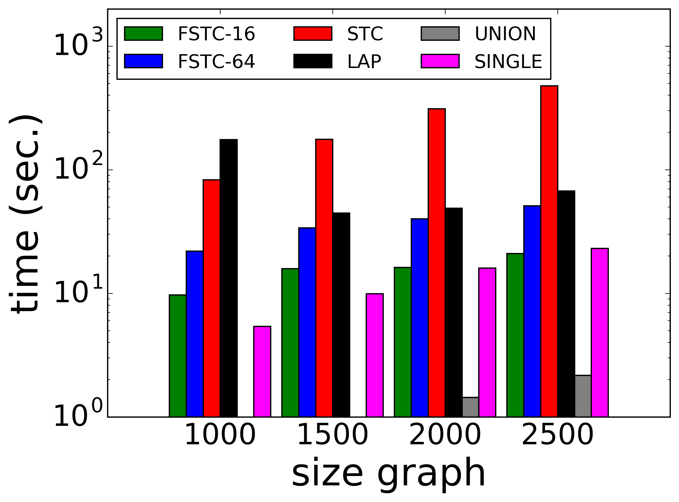
(a) #Vertices

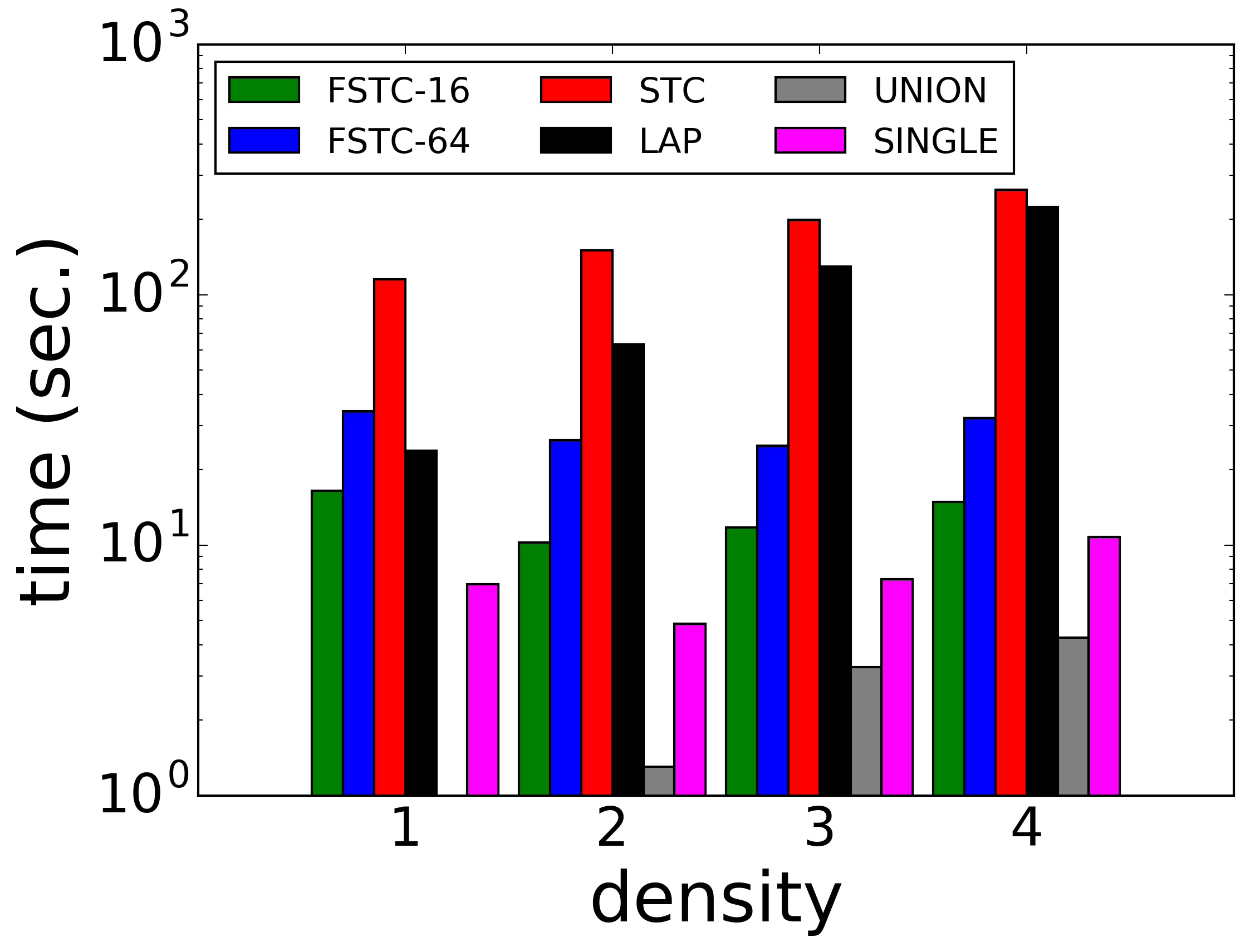
(b) Density

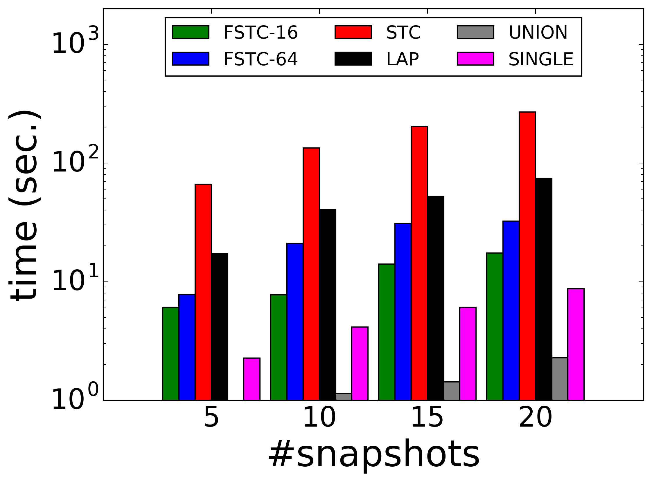
(c) #Snapshots

(d) Rank

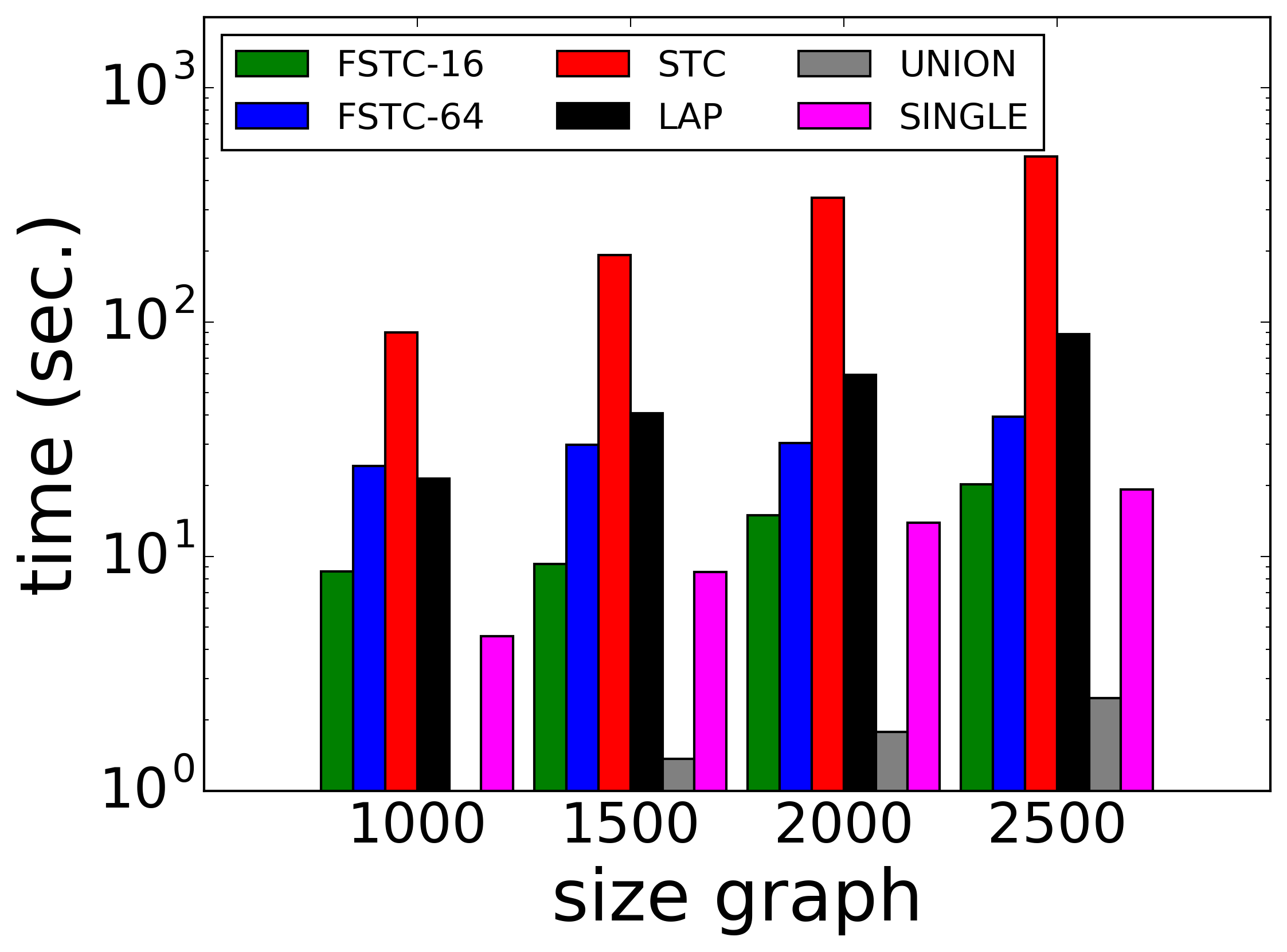
(e) #Vertices

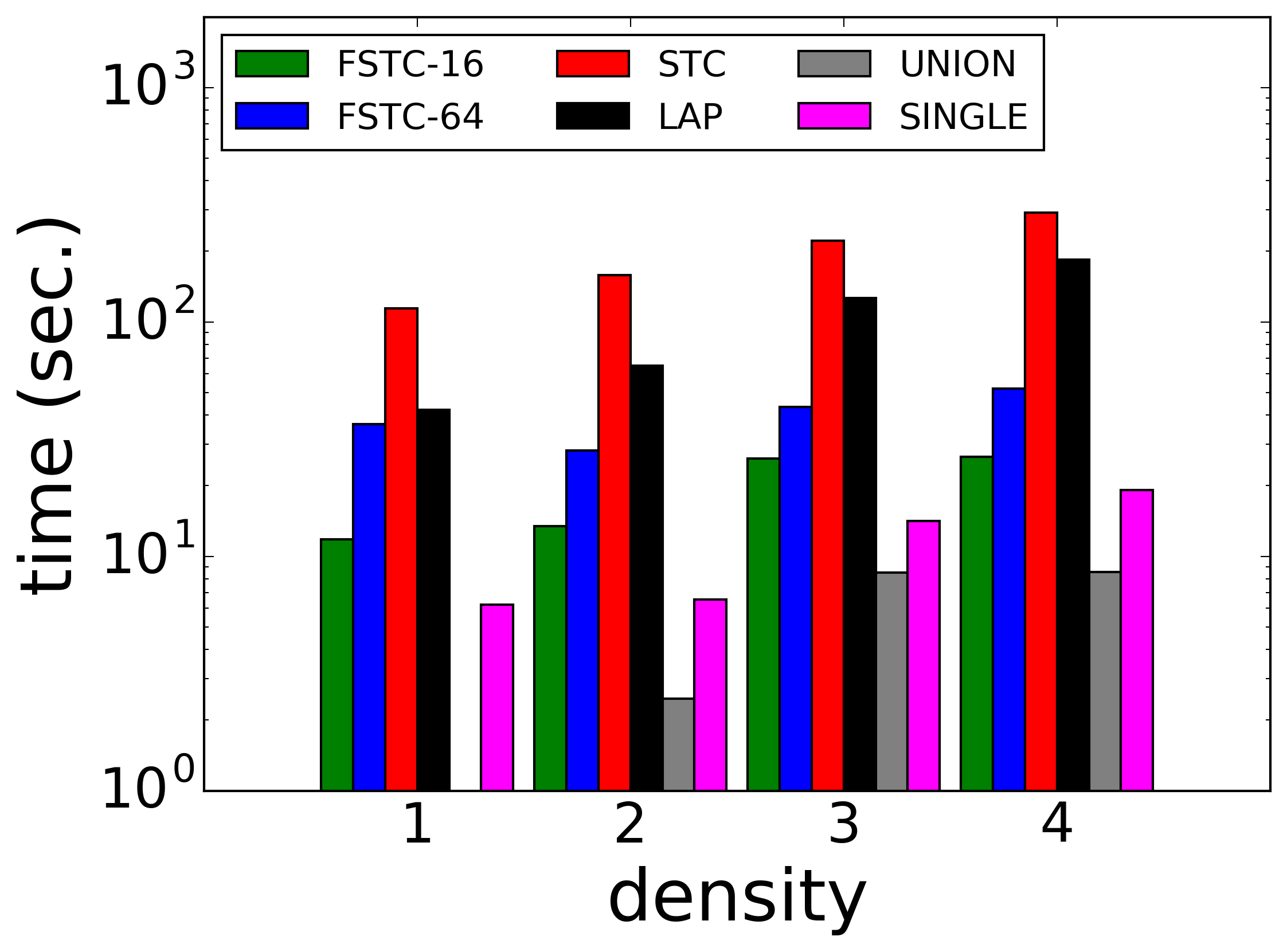
(f) Density

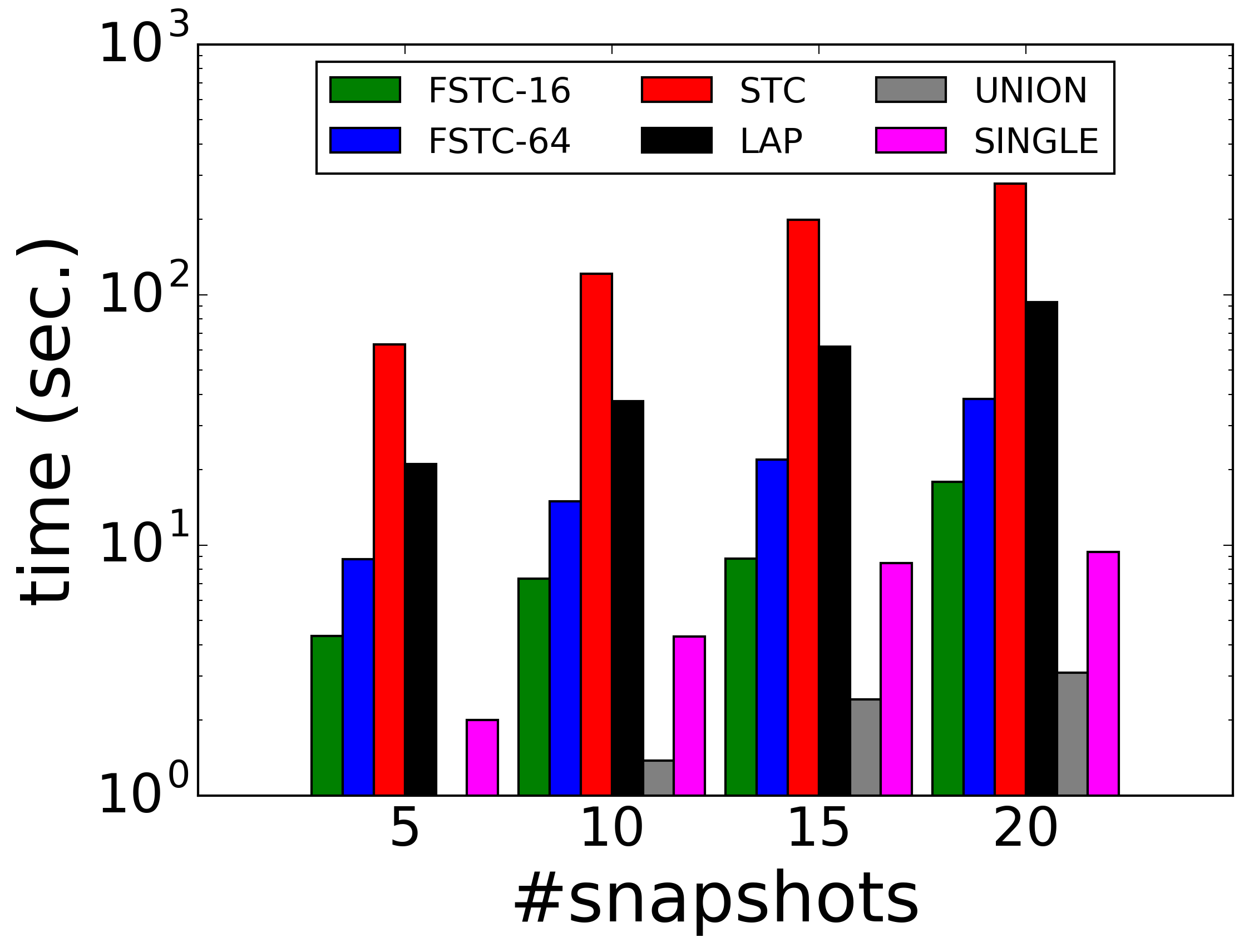
(g) #Snapshots

(h) Rank

Figure 8: Running time results for sparsest (a-d) and normalized (e-h) cuts on synthetic data.

Synthetic heat process over the School network

Figure 9 shows the School-heat dataset. Given Laplacians $L_{0},L_{1}$ and $L_{2}$, associated with the three snapshots, the initial signal $\textbf{f}_{(0)}$ is set to $|V|$ for an arbitrary starting vertex and to $0$ for the remaining vertices. For $t>0$ the signal is computed using the heat equation:

$$\textbf{f}_{(t)}=e^{-tL_{t}}\textbf{f}_{(t-1)}$$ (27)

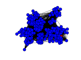
(a) I

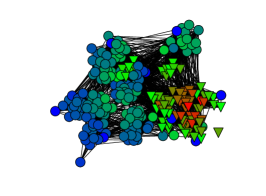
(b) II

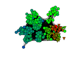
(c) III

Figure 9: School-heat dataset and associated temporal cut (vertex shapes). The dynamic graph signal is generated based on a heat process over the dynamic School network structure. Vertex colors correspond to signal values (red for high and blue for low). Better seen in color.

References

- [1] W. N. Anderson Jr and T. D. Morley. Eigenvalues of the laplacian of a graph. Linear and multilinear algebra, 18(2):141–145, 1985.
- [2] S. Arora, S. Rao, and U. Vazirani. Expander flows, geometric embeddings and graph partitioning. Journal of the ACM, 56(2):5, 2009.
- [3] L. Backstrom, D. Huttenlocher, J. Kleinberg, and X. Lan. Group formation in large social networks: membership, growth, and evolution. In KDD, 2006.
- [4] M. Bazzi, M. A. Porter, S. Williams, M. McDonald, D. J. Fenn, and S. D. Howison. Community detection in temporal multilayer networks, with an application to correlation networks. Multiscale Modeling & Simulation, 14(1):1–41, 2016.
- [5] M. M. Bronstein, J. Bruna, Y. LeCun, A. Szlam, and P. Vandergheynst. Geometric deep learning: going beyond euclidean data. arXiv preprint arXiv:1611.08097, 2016.
- [6] M. Charikar, C. Chekuri, T. Feder, and R. Motwani. Incremental clustering and dynamic information retrieval. In STOC, 1997.
- [7] S. Chen, R. Varma, A. Sandryhaila, and J. Kovačević. Discrete signal processing on graphs: Sampling theory. IEEE Transactions on Signal Processing, 63(24):6510–6523, 2015.
- [8] Y. Chi, X. Song, D. Zhou, K. Hino, and B. L. Tseng. Evolutionary spectral clustering by incorporating temporal smoothness. In KDD, 2007.
- [9] F. R. Chung. Spectral graph theory. American Mathematical Society, 1997.
- [10] J. Cuppen. A divide and conquer method for the symmetric tridiagonal eigenproblem. Numerische Mathematik, 36(2):177–195, 1980.
- [11] S. Fortunato. Community detection in graphs. Physics Reports, 486:75–174, 2010.
- [12] A. Gadde, A. Anis, and A. Ortega. Active semi-supervised learning using sampling theory for graph signals. In KDD, 2014.
- [13] W. N. Gansterer, R. C. Ward, R. P. Muller, and W. A. Goddard III. Computing approximate eigenpairs of symmetric block tridiagonal matrices. SIAM Journal on Scientific Computing, 25(1):65–85, 2003.
- [14] M. Gavish, B. Nadler, and R. Coifman. Multiscale wavelets on trees, graphs and high dimensional data. In ICML, 2010.
- [15] R. Ghosh, S.-h. Teng, K. Lerman, and X. Yan. The interplay between dynamics and networks: centrality, communities, and cheeger inequality. In KDD, 2014.
- [16] D. Greene, D. Doyle, and P. Cunningham. Tracking the evolution of communities in dynamic social networks. In ASONAM, 2010.
- [17] L. Hagen and A. B. Kahng. New spectral methods for ratio cut partitioning and clustering. IEEE Transactions on Computer-aided Design of Integrated Circuits and Systems, 11(9):1074–1085, 1992.
- [18] V. Kawadia and S. Sreenivasan. Sequential detection of temporal communities by estrangement confinement. Scientific reports, 2, 2012.
- [19] R. Kumar, J. Novak, P. Raghavan, and A. Tomkins. On the bursty evolution of blogspace. In WWW, 2003.
- [20] J. Lafferty and G. Lebanon. Diffusion kernels on statistical manifolds. JMLR, 6:129–163, 2005.
- [21] A. N. Langville and C. D. Meyer. Google’s PageRank and beyond: The science of search engine rankings. Princeton University Press, 2011.
- [22] T. Leighton and S. Rao. An approximate max-flow min-cut theorem for uniform multicommodity flow problems with applications to approximation algorithms. In FOCS, 1988.
- [23] J. Leskovec, K. J. Lang, A. Dasgupta, and M. W. Mahoney. Community structure in large networks: Natural cluster sizes and the absence of large well-defined clusters. Internet Mathematics, 6(1):29–123, 2009.
- [24] Y.-R. Lin, Y. Chi, S. Zhu, H. Sundaram, and B. L. Tseng. Facetnet: a framework for analyzing communities and their evolutions in dynamic networks. In WWW, 2008.
- [25] H. Ning, W. Xu, Y. Chi, Y. Gong, and T. S. Huang. Incremental spectral clustering by efficiently updating the eigen-system. Pattern Recognition, 43(1):113–127, 2010.
- [26] A. Sandryhaila and J. Moura. Big data analysis with signal processing on graphs. IEEE Signal Processing Magazine, 31:80–90, 2014.
- [27] J. Shi and J. Malik. Normalized cuts and image segmentation. IEEE Transactions on Pattern Analysis and Machine Intelligence, 22:888–905, 2000.
- [28] D. Shuman, S. Narang, P. Frossard, A. Ortega, and P. Vandergheynst. The emerging field of signal processing on graphs. IEEE Signal Processing Magazine, 2013.
- [29] A. Silva, X. Dang, P. Basu, A. Singh, and A. Swami. Graph wavelets via sparse cuts. In KDD, 2016.
- [30] A. Silva, A. Singh, and A. Swami. Spectral algorithms for temporal graph cuts. http://arxiv.org/abs/1602.03320, 2017.
- [31] A. Sole-Ribalta, M. De Domenico, N. E. Kouvaris, A. Diaz-Guilera, S. Gomez, and A. Arenas. Spectral properties of the laplacian of multiplex networks. Physical Review E, 88(3):032807, 2013.
- [32] D. A. Spielman and S.-H. Teng. Nearly-linear time algorithms for graph partitioning, graph sparsification, and solving linear systems. In STOC, 2004.
- [33] D. A. Spielman and S.-H. Teng. Spectral sparsification of graphs. SIAM Journal on Computing, 40(4):981–1025, 2011.
- [34] J. Stehlé, N. Voirin, A. Barrat, C. Cattuto, L. Isella, J.-F. Pinton, M. Quaggiotto, W. Van den Broeck, C. Régis, B. Lina, et al. High-resolution measurements of face-to-face contact patterns in a primary school. PloS one, 6(8):e23176, 2011.
- [35] D. Taylor, S. A. Myers, A. Clauset, M. A. Porter, and P. J. Mucha. Eigenvector-based centrality measures for temporal networks. arXiv preprint arXiv:1507.01266, 2015.