An Efficient Parallel Data Clustering Algorithm Using Isoperimetric Number of Trees

Abstract

We propose a parallel graph-based data clustering algorithm using CUDA GPU, based on exact clustering of the minimum spanning tree in terms of a minimum isoperimetric criteria. We also provide a comparative performance analysis of our algorithm with other related ones which demonstrates the general superiority of this parallel algorithm over other competing algorithms in terms of accuracy and speed.

Keywords: Isoperimetric number, Cheeger constant, Normalized cut, Graph partitioning

1 Introduction

Data clustering as the unsupervised grouping of similar data which have high intra-similarity and low inter-similarity is one of the most important tasks in many fields such as data mining, signal and image processing, computational biology, computer vision and etc.

In this way, graph-based methods as deriving a weighted graph from data and applying the graph partitioning algorithms is one of the most efficient approaches which has been studied widely in the literature. For a review on various graph-based clustering approaches, see [1] and [2].

Shi and Malik [3] introduced the normalized cut problem (Ncut for short) as an appropriate formulation of the clustering criteria. The objective of the normalized cut problem is to partition the vertex set of a graph into $k$ clusters such that the average of the normalized sparsity of the clusters is minimized. They showed that the decision problem corresponding to the computation of the minimum Ncut of a graph is NP-complete in general and they proposed an approximation procedure (based on spectral techniques) by relaxing the characteristic functions of the clusters into the real domain and using the information provided by the eigenspace of the corresponding Laplacian matrix. Recently, Trevisan et al. [4], by proving higher-order Cheeger’s inequalities, have provided a theoretical justification for the empirical efficiency of the spectral clustering methods.

Daneshgar et al. [5, 6] proved that the normalized cut problem is NP-complete on trees (even unweighted trees) and they proposed to relax the search space from all $k-$partitions to all $k-$subpartitions (a $k-$subpartition is a set of $k$ disjoint subsets of the vertex set which is not necessarily a partition). They achieved a polynomial time algorithm (actually a near linear algorithm) for this relaxed problem (called the isoperimetric problem) on weighted trees and revealed the efficiency of the proposed method applying in the clustering of the real-world data. They also provided some evidence that how the information of residual nodes remained outside the optimal subpartition can be used to extract outlier data points, in the course of performing the clustering process.

In the first step of their algorithm, a weighted graph is created from the data based on some measure of data features. Then, a minimum spanning tree of the graph is computed and the algorithm starts to find $k^{\prime}$th isoperimetric number of the tree. The result is an optimal subpartition of the nodes which yields a clustering of the dataset.

Modifying the standard methods in order to let the computations be performed in parallel can remarkably improve the time performance of the algorithms. Accordingly, this issue, along with the hardware and software development of parallel computation, have been at the center of attention in recent decades. In this paper, we develop an efficient parallel data clustering algorithm based on isoperimetric number of trees. Our approach can be considered as a parallel version of Daneshgar et al. algorithm [6], in which the computational performance is significantly improved.

In recent decades, many parallel computing architectures have been developed falling into two basic categories: CPU based and GPU (Graphics Processor Unit) based architectures. Unlike the CPUs, GPUs are specially developed for running and executing parallel codes, and this feature makes them more powerful and cheaper for performing the computational goals. Also, GPUs have very large memory bandwidth and less data transfer overhead in compare with other parallel architectures (Their memory bandwidth are up to 300 GB/s in recent years). In addition, GPUs have become easy programmable using a high level language, called CUDA, which have been developed for this purpose. Today, GPUs are not only flexible, but also easy programmable devices and this makes them one of the most popular devices for applied and theoretical research purposes (see [7]).

In order to achieve a better performance, we implemented our algorithm on NVidia GPUs by using CUDA platform. The experimental results on real-world datasets reveal a final speed up between 1.36x and 21x. We also show that the efficiency is significantly improved in higher dimensional data such as generated data from social networks. According to the comparison results, we believe that our algorithm is one of the most efficient data clustering algorithms in the case of speed and accuracy.

1.1 Related work

Various algorithms and strategies have been proposed to improve the computational performance of data clustering and its applications to image segmentation, signal processing and etc. In this manner, some attempts have been devoted to develop parallel adaptations of the well-known methods.

K-means is one of the most popular algorithm in data clustering literature. Firstly, Stoffel and Belkoniene [8] developed some parallel techniques for this algorithm. Afterwards, many attempts was devoted to design and implement the parallel version for k-means in the large data sets (e.g. see [9] and [10]).

Normalized cut [3] is another popular graph-based data clustering algorithm for which XianLou and ShuangYuan [11] developed a parallel version and gained about 2.34 times speed up in the best case. In the context of hierarchical clustering, firstly, Olson [12], introduced a parallel algorithm. Also, Dahlhaus [13] presented another parallel algorithm and used his algorithm to solve the undirected split decomposition problem in graphs. Amal Elsayed Aboutabl et al. [14], designed and implemented a parallel document clustering based on hierarchical approach and for the best case, they gained a 5 times speed up over $65\%$ efficiency.

On the other hand, some other parallel algorithms are developed on the various architectures and models. Weizhong et al. [15], implemented a parallel version of k-means clustering on map-reduce model. Middelmann and Sanders [16] proposed a heuristic graph-based image segmentation algorithm and implemented a parallel algorithm for shared-memory machines.

Most of these endeavours are suffered from accuracy and time performance (achievable speed-up in compare with the sequential version).

2 Data clustering: sequential algorithm

2.1 Graph-based clustering

Graph-based data clustering is one of the most important approaches in data clustering. In this approach, the data set is represented as a weighed graph such that each node corresponds to a data point and the weight of each edge between two nodes reflects their proximity. Finally, the clustering problem is reduced to a graph partitioning problem according to a prescribed criteria.

In our model, given a data set $X=\{x_{1},\ldots,x_{n}\}\subseteq\mathbb{R}^{d}$, the corresponding graph is a weighted graph $G$ on the vertex set $X$ and the edge set $E$ (the set of all unordered pairs of $X$) with the following weight functions:

• An edge-weight function $\varphi$ : $E$ $\rightarrow$ $\mathbb{R}^{+}$, called the flow, that represents the similarities between pairs of elements which is defined as,

  $$\forall 1\leq i\neq j\leq n,\ \varphi(x_{i},x_{j}):=\exp(-\|x_{i}-x_{j}\|_{2}/\sigma),$$ (2.1)

  where $\sigma$ is a scaling parameter.

• A vertex-weight function $\omega$ : $X$ $\rightarrow$ $\mathbb{R}^{+}$, stands for the weight of each data element defined as,

  $$\forall 1\leq i\leq n,\qquad\omega(x_{i}):=\sum\limits_{j=1}^{n}\varphi(x_{i},x_{j}).$$ (2.2)

• Another function $p$ : $X$ $\rightarrow$ $\mathbb{R}^{+}\cup\{0\}$ called the potential function which shows the isolation of each data element defined as,

  $$\forall 1\leq i\leq n,\qquad p(x_{i}):=\alpha\sum\limits_{j=1}^{n}\|x_{i}-x_{j}\|_{2},$$ (2.3)

  where $\alpha$ is a scaling factor and is assumed to be equal to zero, unless an extra outlier detection tasks is needed (see [6]).

For a real function $f$ on the set $X$ and a subset $A\subset X$, we define $f(A):=\sum_{x\in A}f(x)$. Also, we denote the boundary of $A$ by $\delta(A)$ and define as,

$$\delta(A):=\{xy\in E\mid x\in A,y\in X\backslash A\}.$$

The collection of all $k$-partitions of $X$ is denoted by $P_{k}(X)$ and defined as,

$$P_{k}(X):=\{ \mathcal{A}=\{A_{1},\ldots,A_{k}\}\mid\forall i,A_{i}\subset X,$$

$$\forall i\neq j,A_{i}\cap A_{j}=\emptyset\text{ and }\bigcup_{i=1}^{k}A_{i}=X\}.$$

Also, the family of all $k$-subpartitions of $X$ is denoted by $D_{k}(X)$ and defined as,

$$D_{k}(X):=\{ \mathcal{A}=\{A_{1},\ldots,A_{k}\}\mid\forall i,A_{i}\subset X,$$

$$\text{ and }\forall i\neq j,A_{i}\cap A_{j}=\emptyset\}.$$

The $k$-normalized cut problem is to find a $k$-partition $\mathcal{A}\in P_{k}(X)$ minimizing the following cost function,

$$\operatorname{cost}(\mathcal{A}):=\max_{1\leq i\leq k}\frac{\varphi(\delta A_{i})+p(A_{i})}{\omega(A_{i})}.$$ (2.4)

Let us define,

$$MNC_{k}(G):=\min_{\mathcal{A}\in P_{k}(X)}\operatorname{cost}(\mathcal{A}).$$ (2.5)

The isoperimetric problem seeks for a minimizer of the cost function in (2.4) over the space of all $k$-subpartitions $D_{k}(X)$. We denote the minimum by $MISO_{k}(G)$ and define as,

$$MISO_{k}(G):=\min_{\mathcal{A}\in D_{k}(X)}\operatorname{cost}(\mathcal{A}).$$ (2.6)

The quotient ($\varphi(\delta A)+p(A))/\omega(A)$ is called the normalized sparsity of the set $A$.

2.2 Sequential algorithm

In [3], it is shown that the normalized cut problem is NP-hard for general graphs (even when $k=2$). Also, in [5] it is shown that this problem is NP-hard on weighed-trees when $k$ is given in the input. In contrast, Daneshgar et al. in [6] shows that the isoperimetric problem is efficiently solvable on weighted tree using a near linear time algorithm. The outline of their method can be described as follows. For a given number $N$, they use Algorithm 1 to check if there exists a subpartition with the cost at most $N$. Then, in order to find the minimizing subpartition, they apply Algorithm 2 which executes a binary search and iteratively calls Algorithm 1 as a subroutine. In fact, Algorithm 1 is essentially a backtracking which traverses through the vertices and check if a vertex can be either cut from or join to its parent, according to some sort of conditions.

The detail of Algorithms 1 and 2 are elaborated in the following. To prove the correctness of Algorithms 1 and 2, see [6].

Algorithm 1
Input: A weighted tree ($T,\omega,\varphi,p$) rooted at the vertex $v$, an integer $k$ and a rational number $N$. (It is assumed that the vertices are ordered in BFS order as $x_{1},\ldots,x_{n}=v$.)
Output: A $k$-subpartition $\mathcal{A}\in D_{k}(X)$ (if there exists) such that $\operatorname{cost}(\mathcal{A})\leq N$ as in (2.4).

Initialize the set function $\eta$ : $X$ $\rightarrow$ $P(X)$ by $\eta(x_{i})$ = {$x_{i}$} for each $1\leq i\leq n$.

Define $i$ = 1 , $j$ = 0.

while $j<k$ and $i\leq n$ do

     Let $u$ be the parent of $x_{i}$ and $e=x_{i}u\in E$ be the parent edge.

     if $\varphi(e)+p(x_{i})\leq N\omega(x_{i})$  then

         $j\leftarrow j+1$, $A_{j}\leftarrow\eta(x_{i})$, $\omega(A_{j})\leftarrow\omega(x_{i})$

         $\varphi(\delta A_{j})\leftarrow\varphi(e)+p(x_{i})$, $p(u)\leftarrow p(u)+\varphi(e)$.

     else if $p(x_{i})-\varphi(e)<N\omega(x_{i})$ then

         $\eta(u)\leftarrow\eta(u)\cup\eta(x_{i})$, $\omega(u)\leftarrow\omega(u)+\omega(x_{i})$, $p(u)\leftarrow p(u)+p(x_{i})$.

     else

         $p(u)\leftarrow p(u)+\varphi(x_{i})$.

     end if

     $i\leftarrow i+1$.

end while

if $j$ = $k$ then

     return YES and $\mathcal{A}=\{A_{1},\ldots,A_{k}\}$.

else

     return NO.

end if

Now, suppose that $\varphi^{*}$, $\varphi_{*}$, $p^{*}$, $p_{*}$, $\omega^{*}$ and $\omega_{*}$ are defined as follows.

$$\varphi^{*} :=\sum\limits_{e\in E}\varphi(e),\hskip 50.0pt \varphi_{*}:=\min\limits_{e\in E}\varphi(e),$$

$$\omega^{*} :=\sum\limits_{x\in X}\omega(x),\hskip 50.0pt \omega_{*}:=\min\limits_{x\in X}\omega(x),$$

$$p^{*} :=\sum\limits_{x\in X}p(x),\hskip 50.0pt p_{*}:=\min\limits_{x\in X}p(x).$$

Algorithm 2 finds the minimizing subpartition.

Algorithm 2
Input: A rooted weighted tree ($T,\omega,\varphi,p$), an integer $k$.
Output: A minimizing subpartition achieving $MISO_{k}(T)$.

Let $\alpha_{0}\longleftarrow\frac{\varphi_{*}+p_{*}}{\omega^{*}}$ and $\beta_{0}\longleftarrow\frac{\varphi^{*}+p^{*}}{\omega_{*}}$.

Let $t\longleftarrow\log(2{\omega^{*}}^{2}(\beta_{0}-\alpha_{0}))-\log(\varphi_{*}+p_{*})$.

Initialize $\alpha\longleftarrow\alpha_{0}$ and $\beta\longleftarrow\beta_{0}$.

for $i=1$ to $t$ do

     Applying Algorithm 1, decide if $MISO_{k}(T)\leq\ \frac{\alpha+\beta}{2}$.

     if  $MISO_{k}(T)\leq\ \frac{\alpha+\beta}{2}$ then

         $\beta\longleftarrow\frac{\alpha+\beta}{2}$.

     else

         $\alpha\longleftarrow\frac{\alpha+\beta}{2}$.

     end if

end for

Let $\mathcal{A}$ be the $k$-subpartition output of Algorithm 1 for deciding $MISO_{k}(T)\leq\beta$.

return $MISO_{k}(T)=\operatorname{cost}(\mathcal{A})$ and $\mathcal{A}$.

According to the procedures, the main steps of the sequential data clustering algorithm, can be summarized as follows.

1. Given the dataset of vectors $X$, construct the affinity graph $G$ on $X$ along with the edge weights $d(x_{i},x_{j})=\|x_{i}-x_{j}\|_{2}$.
   

2. Find a minimum spanning tree $T$ for $(G,d)$ and calculate the functions $\varphi$, $\omega$ and $p$ for $T$.
   

3. Order the vertices of $T$ in BFS order and determine the parent for each vertex.
   

4. Calculate $\varphi^{*}$, $\varphi_{*}$, $p^{*}$, $p_{*}$, $\omega^{*}$ and $\omega_{*}$.
   

5. Apply Algorithm 2, iteratively call Algorithm 1 and find $MISO_{k}(T)$ with the minimizing subpartition $\mathcal{A}\in D_{k}(X)$.

3 Structure of parallel clustering algorithm

In this section, firstly we give a brief description of NVIDIA CUDA architecture and programming model. Then we explain our data structures and some preliminaries. Finally, we propose our parallel data clustering algorithm in detail.

3.1 GPGPU and CUDA programming model

In last two decades, improving the performance of the computer processors is generally achieved by increasing the clock rate, however this improvement is restricted by the physical limitations. Therefore, a large amount of research have been concentrated on parallelism by using multi-processors (instead of one processor).

Today, the graphics processors (GPU) have been evolved into the powerful and flexible processors that are designed to perform calculations on large amount of independent data concurrently. General-purpose computing on graphics processing units, GPGPU, refers to the use of GPU for the mathematical and scientific computing tasks.

CUDA is a software development kit (SDK), which has been developed by NVIDIA Corporation, used for writing programs on their GPUs and allows for the execution of C functions on graphics card.

The CUDA programming model is based on executing parallel threads concurrently. CUDA manages threads in a hierarchical structure. A collection of threads (called a block) are run on a multiprocessor, which contains a number of processors, at a given time. The collection of all blocks in a single execution is called a grid. All threads in one grid share the same functionality, as they are being executed the same kernel code in multiple directions. Also, CUDA has a hierarchical memory model. In this model, each thread has a local memory. The threads of a single block share a fast-accessible memory which is called the shared memory. Also, all threads in different blocks can communicate through a low-speed global memory. This model provides a powerful platform for scientific computing objectives. (Figure 1)

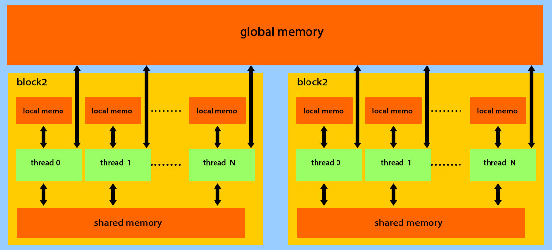
Figure 1: CUDA memory model

3.2 Principles and definitions

The main essence of Algorithm 1 is to check each vertex separately if it can be either cut from or join to its unique parent using the specific conditions. Thus, it is not hard to see that at each depth in the tree, all vertices can be considered independently and simultaneously. This is the crucial point in paralleling Algorithm 1. Based on this idea, we can describe our parallel data clustering algorithm as follows.

1. Given the dataset $X$, construct the affinity graph $(G,d)$ in parallel.

2. Using Algorithm 3, find the minimum spanning tree $T$ and the BFS order of the vertices.

3. Calculate the parameters $\varphi^{*}$, $\varphi_{*}$, $p^{*}$, $p_{*}$, $\omega^{*}$, and $\omega_{*}$.

4. Start from the lowest depth and check the conditions of Algorithm 1 for all vertices in that depth simultaneously.

In the rest of this section, we describe each step of the algorithm in detail.

3.3 Graph representations and data structures

The standard data structure for graph representation are mainly the adjacency matrix and the adjacency list [17] (Figure 2).

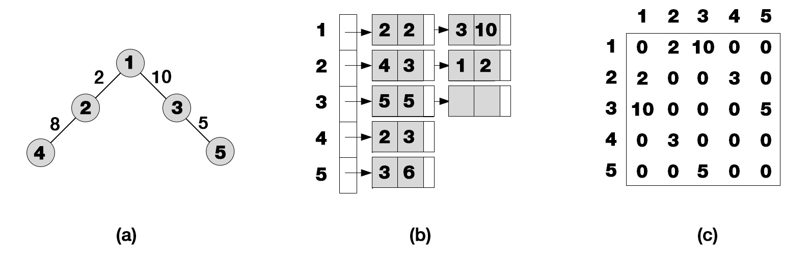
Figure 2: Standard graph representations.

In the adjacency matrix of $G(V,E)$, we need $O(|V|^{2})$ space which is used for constructing an affinity matrix of the graph, where $G_{ij}$ shows the edge weight between two vertices $i$ and $j$. On the other hand, the adjacency list of a graph $G(V,E)$ consists of an array $A$ of lists of size $|V|$, one for each vertex in $V$ and for each $u\in V$ the adjacency list of $u$, $A[u]$ contain all neighbours of $u$ and their edge weights.

In our implementation, we use the adjacency matrix for constructing fully connected graph in order to access every edge weight for calculating the minimum spanning tree in $O(1)$. Also, we used a new data structure to represent the rooted tree called parent list which consists of two arrays $A$ and $W$ with size $|V|$, and for each vertex $u\in V(G)$, $A[u]$ contains the parent of $u$ and $W[u]$ saves the edge weight $\varphi({uv})$, where $v$ is the unique parent of $u$ (Figure 3).

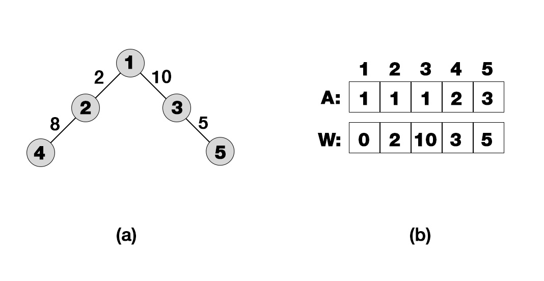
Figure 3: Parent List.

This data structure is more useful in the way that it is linear space bounded and the edge weights can be obtained in the constant time.

3.4 Finding affinity matrix

The parallel implementation for calculating the affinity matrix is one of the easiest steps in our algorithm. For calculating the distances of the pairs is totally independent, for each pair $(i,j)$ of vertices, one thread computes the corresponding weight $d(i,j)$ independently and the total number of launched threads is $\frac{n(n+1)}{2}$.

3.5 Finding the minimum spanning tree and the weight functions

Finding the minimum spanning tree (MST) is one of the most important and most studied problems in combinatorial optimization. It has many applications in different fields such as networking, VLSI layout and routing, computational biology and etc.

Formally, a minimum spanning tree of an undirected connected graph $G(V,E)$ with vertices $V=\{v_{1},\ldots,v_{n}\}$ and weighed edges $E$, can be defined as a connected subgraph of $G$ that contains all vertices and $n-1$ edges with the minimum total weights.

The most well-known sequential MST algorithms are Kruskal, Prim and Boruvka algorithm [17]. In [18], Wang et al. showed that compared to the other parallel MST algorithms, parallel implementation of Prim’s algorithm is incomparably slower. This is due to the fact that in Prim’s algorithm, the vertices are added to the tree sequentially. Nevertheless, Prim’s algorithm is more useful for our purpose in the way that by adding vertices sequentially, we can determine some information including the parent and depth functions at the same time for each vertex. This information can lead us to omit the BFS part of the algorithm.

In addition, Wang et al. [18] proposed a parallel version of the Prim’s algorithm and showed that their algorithm can be implemented efficiently on GPUs using min-reduction primitive (for more information about the parallel implementation of reduction algorithms see [19]).

Based on their approach, our parallel implementation of Prim’s algorithm can described as follows:

Algorithm 3
Input: A weighted complete graph $(G,d)$ and a root vertex $v$.
Output: The minimum spanning tree rooted at $v$ and the parent and depth functions.

1:Initialize $T=\{\emptyset\}$.

2:Add the root vertex $v$ to the tree and save the distance between $v$ and the other vertices.

3:while $|T|\leq n$ do

4:     Find the vertex outside $T$ with the minimum distance to $T$ using min-reduction algorithm.

5:     Add new vertex to $T$ and save its Parent and Depth.

6:     Update all distances simultaneously.

7:end while

After calculating the minimum spanning tree, we apply a min-reduction algorithm to find the numbers $\varphi_{*}$, $p_{*}$, $\omega_{*}$ and sum-reduction algorithm to calculate $\varphi^{*}$, $p^{*}$, $\omega^{*}$.

3.6 Computing the isoperimetric number

One may observe that Algorithm 1 is a search algorithm which starts by traversing vertices in the BFS order and decides to join or separate the vertices from their parents. Finally, it returns the suitable clusters (if exist). A vertex which is separated from its parent due to the conditions of Algorithm 1 is called a cut vertex. We define two arrays $Cut$ and $\eta$ of size $n$ as follows. For every $i\in\{1,\ldots,n\}$, define

$$Cut(i)=\left\{\begin{array}[]{ll}1&\text{ if }x_{i}\text{ is a cut vertex},\\ 0&\text{otherwise}.\end{array}\right.$$

Also, at the end of Algorithm 1, if $x_{j}$ is the vertex of the lowest depth which is joint with $x_{i}$, then define $\eta(i)=j$. The arrays $Cut$ and $\eta$ can be computed after checking the condition during the execution of Algorithm 1.

As mentioned above, in the parallel version, we check the conditions of Algorithm 1 depth-by-depth. Figure 4 shows the overall design flow diagram. Also, during the CUDA implementation, we use some techniques which significantly improve the performance of the program. In the following, we will describe the details of these techniques.

1. Since it is impossible to write on a single memory location in parallel at the same time, after checking the conditions of Algorithm 1 at each depth, we try to sequence all vertices belonging to this depth with a common parent. We save this sequence for the whole vertices in an array called $ChildId$ which can be obtained during MST computation step (in Algorithm 3). Then, we use this array to prevent the conflict between the threads. Therefore, we can operate all vertices with the same $ChildId$ in parallel.

2. Writing step is the most expensive part in the algorithm and based on this fact, we try to exchange the algorithm steps to reduce the execution number of this task. For this purpose, after checking the conditions, firstly, we calculate the number of clusters that can be obtained and just execute the adding step if we have not achieved $k$ clusters.

3. The final output of the data clustering algorithms is an array in size of the data containing a cluster label for each single element. Since, this array is just needed in the final step, we do not calculate these labels in the intermediate steps. Instead, at each step, we just save the arrays $\eta$ and $Cut$ (defined above) and we use them to produce the final labels, at the end of the Algorithm 2.

4. Having two arrays $\eta$ and $Cut$ is sufficient to obtain the cluster labels for all elements. We designed an efficient procedure to calculate these labels by applying the parallel exclusive scan operation on $Cut$ array in the last step of Algorithm 2. (For more information about the parallel implementation of the exclusive scan algorithm see [20].)

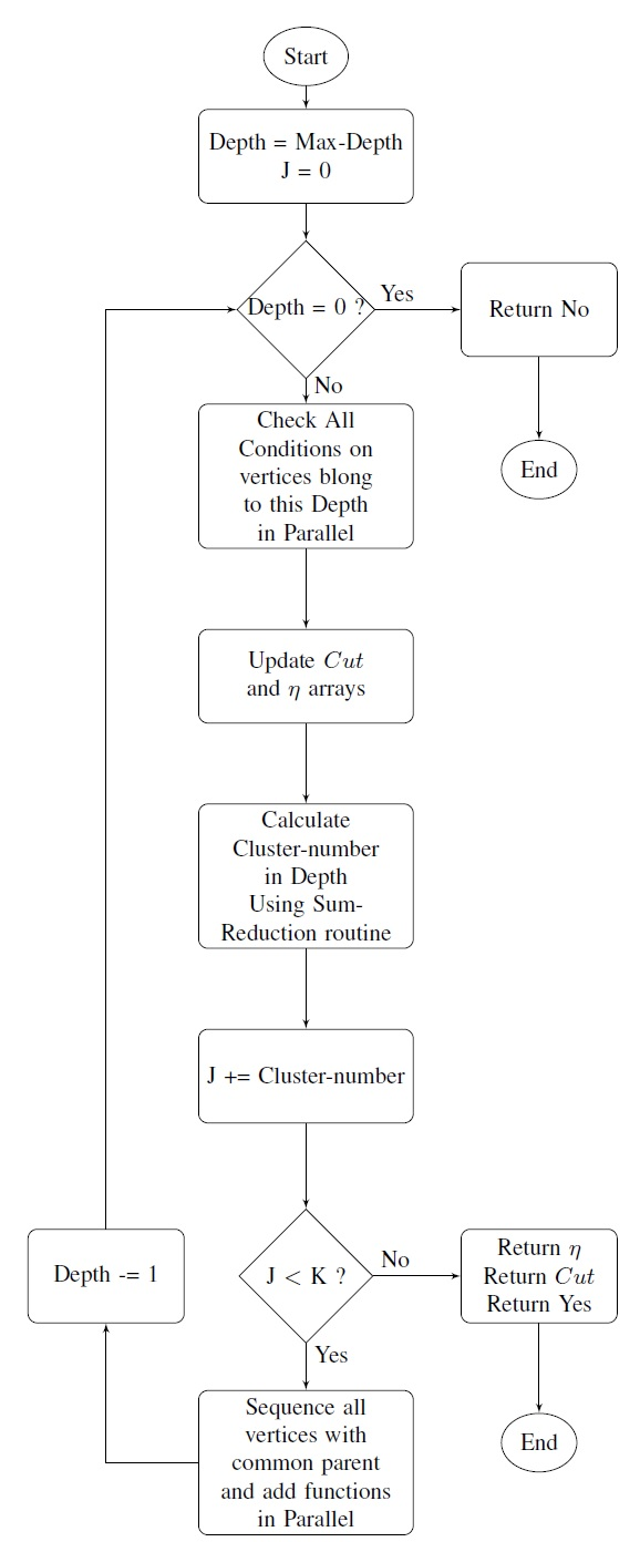
Figure 4: Overall design flow diagram of the parallel implementation of Algorithm 1.

Based on these facts, in Algorithm 4, we provide a parallel implementation of Algorithm 2.

Algorithm 4
Input: A weighted tree ($T,\omega,\varphi,p$) and an integer $k$.
Output: A minimizer achieving $MISO_{k}(T)$.

Let $\alpha_{0}\longleftarrow\frac{\varphi_{*}+p_{*}}{\omega^{*}}$ and $\beta_{0}\longleftarrow\frac{\varphi^{*}+p^{*}}{\omega_{*}}$.

Let $t\longleftarrow\log(2\omega^{*^{2}}(\beta_{0}-\alpha_{0}))-\log(\varphi_{*}+p_{*})$.

Initialize $\alpha\longleftarrow\alpha_{0}$ and $\beta\longleftarrow\beta_{0}$

for $i=1$ to $t$ do

     Apply the parallel algorithm and decide if $MISO_{k}\leq\ \frac{\alpha+\beta}{2}$.

     if  $MISO_{k}\leq\ \frac{\alpha+\beta}{2}$ then

         Save $Cut$ and $\eta$;

         $\beta\longleftarrow\frac{\alpha+\beta}{2}$

     else

         $\alpha\longleftarrow\frac{\alpha+\beta}{2}$

     end if

end for

Initialize the array $\psi$ by $\psi(j)=0$ and the set $A_{j}$ by $A_{j}=\emptyset$, for every $1\leq j\leq k$.

Apply Exclusive Scan algorithm on $Cut$ and save in $ScanArray$.

for all $1\leq i\leq n$ in parallel  do

     if $Cut({i})=1$ then

         $\psi(ScanArray({i}))={i};$

     end if

end for

for $j=1$ to $k$  do

     for all $1\leq{i}\leq n$ in parallel  do

         if $\eta({i})=\psi(j)$ then

              $A_{j}=A_{j}\cup\{x_{i}\};$

         end if

     end for

end for

return $MISO_{k}(T)$ and $\mathcal{A}=\{A_{1},\ldots,A_{k}\}$.

4 Analysis and experimental results

In this section, at first, we investigate the time complexity analysis of the algorithm and then we illustrate the performance of our algorithm on various synthetic and real datasets.

4.1 Time Complexity Analysis

According to the previous sections, the phases of our algorithm can be summarized as follows.

1. Adjacency matrix computation.
   In the sequential algorithm, the computation of the adjacency matrix in global scale needs $O(n^{2})$ time to calculate all the edge weights. In our implementation each weight is calculated by a single thread. Thus, the time complexity is $O(1)$.

2. Finding the minimum spanning Tree $T$.
   The running time of Prim’s algorithm is $O(n^{2})$ in the sequential implementation [17]. In our implementation, we begin with an empty tree and at each step, we use the min-reduction algorithm to find the nearest vertex. The step-complexity of the min-reduction algorithm is known to be $O(\log n)$ [19]. Therefore, the parallel implementation of Prim’s Algorithm is $O(n\log n)$ [18].

3. Tree Partitioning
   In [6], it is shown that the time complexity of Algorithm 2 is $O(n\log n)$. In our parallel implementation of Algorithm 1, we traverse the tree depth-by depth. At each depth firstly, we check all the conditions simultaneously which takes $O(1)$ time. Then, we sequence all vertices with a common parent and execute the operations. Thus, the running time of the parallel algorithm is $O(n)$ and the time complexity of parallel tree partitioning algorithm is $O(n\log n)$ in the worst case.
   It should be noted that the worst time occurs when all vertices are connected directly to the root and this case is too far from the real instances.

4.2 Experimental Results

In this section, we compare the running time of our GPU and CPU implementations of the clustering algorithm. The computer used is equipped with Intel i7 3GHz CPU. It runs Linux Ubuntu and has 12GB of main memory. The GPU used is the NVIDIA GTX850M with 640 processing cores and 4 GB device memory and CUDA SDK 5.0 is used in our GPU implementation.

Table 1 lists the datasets information and shows the performance of our Parallel implementation (GPU) with respect to the sequential implementation (CPU).

Table 1: Performance on UCI database. Symbols n,k,d stand for the size of dataset, number of clusters and number of attributes (i.e. dimension).

Data Set	$n$	$k$	$d$	CPU(ms)	GPU (ms)	Speed-Up	Misclassification rate
Wine	178	3	13	12.51	58.40	0.21x	0.281
Skin	2000	2	3	373	311	1.19x	0.014
Yeast	1484	10	8	323	237	1.36x	0.686
Wine Quality	4898	10	11	4161	743	5.6x	0.844
Internet Advertisements	3279	2	1558	177291	8483	20.89x	0.482

Also, we have considered the performance of our algorithm on a number of randomly generated problems in low and high dimensions. Figures 5 and 6 shows the performance for the data of high dimension ($d=40$) and low dimension ($d=5$), respectively.

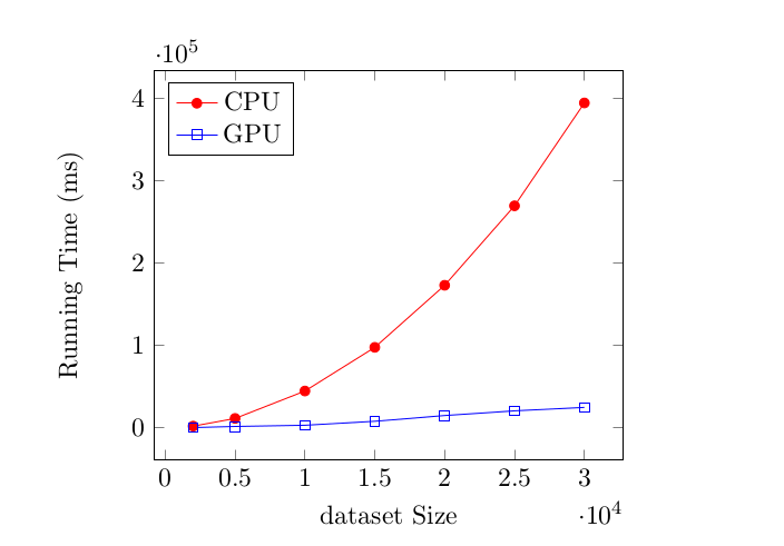
Figure 5: Experiments on randomly generated data sets with high-dimensional data $(d=40)$.

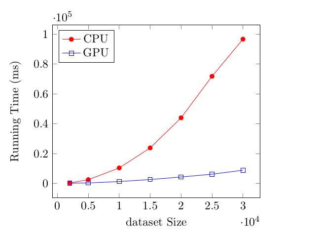
Figure 6: Experiments on randomly generated datasets with low-dimensional data.

5 Conclusion And Future Work

In this paper, we presented an efficient parallel data clustering algorithm based on the isoperimetric number of trees on GPU using CUDA. Firstly, we showed how to parallelize the procedure of computing adjacency matrix, the minimum spanning tree, and other preprocesses. Then, we described our parallel algorithm for tree partitioning and some tricks to increase its performance. Experiments show the efficiency of our algorithm in the way of speed and accuracy.

It should be noted that our algorithm is faced with the limitation of memory for large scale data sets on GPUs. So, it seems necessary to design a procedure to overcome this problem in the future work.

References

- [1] A. K. Jain, M. N. Murty, P. J. Flynn, Data clustering: a review, ACM computing surveys (CSUR) 31 (3) (1999) 264–323.
- [2] R. Xu, D. Wunsch, et al., Survey of clustering algorithms, Neural Networks, IEEE Transactions on 16 (3) (2005) 645–678.
- [3] J. Shi, J. Malik, Normalized cuts and image segmentation, Pattern Analysis and Machine Intelligence, IEEE Transactions on 22 (8) (2000) 888–905.
- [4] J. R. Lee, S. O. Gharan, L. Trevisan, Multiway spectral partitioning and higher-order cheeger inequalities, Journal of the ACM (JACM) 61 (6) (2014) 37.
- [5] A. Daneshgar, R. Javadi, On the complexity of isoperimetric problems on trees, Discrete Applied Mathematics 160 (1) (2012) 116–131.
- [6] A. Daneshgar, R. Javadi, S. S. Razavi, Clustering and outlier detection using isoperimetric number of trees, Pattern Recognition 46 (12) (2013) 3371–3382.
- [7] J. D. Owens, D. Luebke, N. Govindaraju, M. Harris, J. Krüger, A. E. Lefohn, T. J. Purcell, A survey of general-purpose computation on graphics hardware, in: Computer graphics forum, Vol. 26, Wiley Online Library, 2007, pp. 80–113.
- [8] K. Stoffel, A. Belkoniene, Parallel k/h-means clustering for large data sets, in: Euro-Par’99 Parallel Processing, Springer, 1999, pp. 1451–1454.
- [9] I. S. Dhillon, D. S. Modha, A data-clustering algorithm on distributed memory multiprocessors, in: Large-Scale Parallel Data Mining, Springer, 2000, pp. 245–260.
- [10] M. N. Joshi, Parallel k-means algorithm on distributed memory multiprocessors, Computer Science.
- [11] H. XianLou, Y. ShuangYuan, Image segmentation based on normalized cut and cuda parallel implementation, in: Wireless, Mobile and Multimedia Networks (ICWMMN 2013), 5th IET International Conference on, IET, 2013, pp. 209–214.
- [12] C. F. Olson, Parallel algorithms for hierarchical clustering, Parallel computing 21 (8) (1995) 1313–1325.
- [13] E. Dahlhaus, Parallel algorithms for hierarchical clustering and applications to split decomposition and parity graph recognition, Journal of Algorithms 36 (2) (2000) 205–240.
- [14] A. E. Aboutabl, M. N. Elsayed, A novel parallel algorithm for clustering documents based on the hierarchical agglomerative approach, Int. J. Comput. Sci. Inf. Technol.(IJCSIT) 3 (2) (2011) 152–163.
- [15] W. Zhao, H. Ma, Q. He, Parallel k-means clustering based on mapreduce, in: Cloud Computing, Springer, 2009, pp. 674–679.
- [16] J. Wassenberg, W. Middelmann, P. Sanders, An efficient parallel algorithm for graph-based image segmentation, in: Computer Analysis of Images and Patterns, Springer, 2009, pp. 1003–1010.
- [17] T. H. Cormen, C. E. Leiserson, R. L. Rivest, C. Stein, et al., Introduction to algorithms, Vol. 2, MIT press Cambridge, 2001.
- [18] W. Wang, Y. Huang, S. Guo, Design and implementation of GPU-based Prim’s algorithm, International Journal of Modern Education and Computer Science (IJMECS) 3 (4) (2011) 55.
- [19] M. Harris, et al., Optimizing parallel reduction in cuda, NVIDIA Developer Technology 2 (4).
- [20] M. Harris, S. Sengupta, J. D. Owens, Parallel prefix sum (scan) with cuda, GPU gems 3 (39) (2007) 851–876.