Spectral methods for Langevin dynamics and associated error estimates

Julien Roussel and Gabriel Stoltz
Université Paris-Est, CERMICS (ENPC), Inria, F-77455 Marne-la-Vallée, France
Abstract

We prove the consistency of Galerkin methods to solve Poisson equations where the differential operator under consideration is hypocoercive. We show in particular how the hypocoercive nature of the generator associated with Langevin dynamics can be used at the discrete level to first prove the invertibility of the rigidity matrix, and next provide error bounds on the approximation of the solution of the Poisson equation. We present general convergence results in an abstract setting, as well as explicit convergence rates for a simple example discretized using a tensor basis. Our theoretical findings are illustrated by numerical simulations.

Key words.

Langevin dynamics, spectral methods, Poisson equation, error estimates

2000 Mathematics Subject Classification.

82C31, 35H10, 65N35

1 Introduction

Statistical physics gives a theoretical framework to bridge the gap between microscopic and macroscopic descriptions of matter [4]. This is done in practice with numerical methods known as molecular simulation [2, 11, 32, 21]. Despite its intrinsic limitations on spatial and timescales, molecular simulation has been used and developed over the past 50 years, and recently gained some recognition through the 2013 Chemistry Nobel Prize. One important aim of molecular dynamics is to quantitatively evaluate macroscopic properties of interest, obtained as averages of functions of the full microstate of the system (positions and velocities of all atoms in the system) with respect to some probability measure, called thermodynamic ensemble. Some properties of interest are static (a.k.a. thermodynamic properties): heat capacities; equations of state relating pressure, density and temperature; etc. Other properties of interest include some dynamical information. This is the case for transport coefficients (such as thermal conductivity, shear viscosity, etc) or time-dependent dynamic properties such as Arrhenius constants which parametrize chemical kinetics.

From a technical viewpoint, the computation of macroscopic properties requires in any case the sampling of high-dimensional measures. We consider in this work the computation of properties in the canonical ensemble, characterized by the Boltzmann–Gibbs measure, which models systems at constant temperature. One popular way to sample the canonical ensemble is provided by the Langevin dynamics. Denoting by D𝐷D the dimension of the system, by q𝒟𝑞𝒟q\in\mathcal{D} the positions of the particles in the system and by pD𝑝superscript𝐷p\in\mathbb{R}^{D} their momenta, the Langevin dynamics reads

{dqt=ptmdt,dpt=(V(qt)γptm)dt+2γβdWt,\left\{\begin{aligned} \differential q_{t}&=\frac{p_{t}}{m}\,\differential t,\\ \differential p_{t}&=\left(-\nabla V(q_{t})-\gamma\frac{p_{t}}{m}\right)\,\differential t+\sqrt{\frac{2\gamma}{\beta}}\,\differential W_{t},\end{aligned}\right. (1)

where β>0𝛽0\beta>0 is proportional to the inverse temperature, m>0𝑚0m>0 is the mass of the particles111Our results can be extended to the case of any symmetric positive definite mass matrix M𝑀M but we focus on the case when M𝑀M is proportional to the identity matrix for simplicity., γ>0𝛾0\gamma>0 is the friction coefficient and Wtsubscript𝑊𝑡W_{t} is a standard Brownian motion in dimension D𝐷D. The potential energy V:𝒟:𝑉𝒟V:\mathcal{D}\rightarrow\mathbb{R} is supposed to be a smooth function. In practice, 𝒟𝒟\mathcal{D} is either a compact domain with periodic boundary conditions, as for example 𝒟=(a𝕋)D𝒟superscript𝑎𝕋𝐷\mathcal{D}=(a\mathbb{T})^{D} where 𝕋=/𝕋\mathbb{T}=\mathbb{R}/\mathbb{Z} is the unit torus and a>0𝑎0a>0 denotes the size of the simulation cell; or the unbounded space 𝒟=D𝒟superscript𝐷\mathcal{D}=\mathbb{R}^{D}. When eβVsuperscripte𝛽𝑉\mathrm{e}^{-\beta V} is integrable, the Langevin dynamics admits as a unique invariant measure the canonical measure

μ(dqdp)=Zβ,μ1eβH(q,p)dqdp,H(q,p)=V(q)+|p|22m,formulae-sequence𝜇𝑞𝑝superscriptsubscript𝑍𝛽𝜇1superscripte𝛽𝐻𝑞𝑝𝑞𝑝𝐻𝑞𝑝𝑉𝑞superscript𝑝22𝑚\mu(\differential q\,\differential p)=Z_{\beta,\mu}^{-1}\mathrm{e}^{-\beta H(q,p)}\,\differential q\,\differential p,\qquad H(q,p)=V(q)+\frac{|p|^{2}}{2m}, (2)

where the partition functions Zβ,μsubscript𝑍𝛽𝜇Z_{\beta,\mu} is a normalization coefficient.

In several situations, one is interested in solutions of Poisson equations of the form

Φ=R𝔼μ[R],Φ𝑅subscript𝔼𝜇delimited-[]𝑅-\mathcal{L}\Phi=R-\mathbb{E}_{\mu}[R], (3)

where \mathcal{L} denotes the generator of the Langevin dynamics (1). For instance, asymptotic variances of ergodic averages or transport coefficients can be written as

𝒟×D1(R𝔼μ[R])Sdμsubscript𝒟superscript𝐷superscript1𝑅subscript𝔼𝜇delimited-[]𝑅𝑆𝜇\int_{\mathcal{D}\times\mathbb{R}^{D}}-{\mathcal{L}^{-1}}\left(R-\mathbb{E}_{\mu}[R]\right)S\,\differential\mu (4)

for some functions R𝑅R and S𝑆S. For the asymptotic variance related to the time average of an observable R𝑅R, one has S=2R𝑆2𝑅S=2R. For transport coefficients, R𝑅R would be the system response whereas S𝑆S is the conjugate response (see for instance the presentation in [23, Section 5]). In practice, quantities such as (4) are evaluated by Monte Carlo strategies, where the quantity of interest is rewritten as the integral of a time-dependent correlation function (the famous Green–Kubo formula), which is approximated by independent realizations of the process. In some cases however, spectral methods are used to solve the Poisson equation (3), see for instance [29, 20, 28, 24].

The error analysis associated with spectral Galerkin methods faces several difficulties. The most important one probably is that the generator \mathcal{L} of the Langevin dynamics is not an elliptic operator, and that it is not naturally associated with a quadratic form. Many approximation results exist for elliptic operators, see for instance [6]. In the context of molecular dynamics, elliptic operators correspond to overdamped Langevin dynamics, which are effective dynamics on the positions only. A Lax-Milgram theorem holds for the quadratic form associated with the generator of the overdamped Langevin dynamics, which makes it possible to quantify the error on the solution of Poisson equations, as recently done in [1]. In contrast, the generator \mathcal{L} of the Langevin dynamics (1) is invertible but not coercive, so that a dedicated treatment is required to obtain error estimates. This is done here by a perturbation of the proof of invertibility obtained as a corollary of the decay estimates provided in [7, 8], which builds on the theory of hypocoercivity [33]. Note that this proof applies to a large class of hypocoercive operators. In this work we restrict ourselves to the Langevin dynamics, the proofs being directly transposable for operators satisfying the hypotheses presented in [8]. Let us also mention previous results on the numerical analysis of hypocoercive operators, relying on finite element or finite difference methods, and providing finite time estimates [10, 26].

This article is organized as follows. We first recall some fundamental properties of the Langevin dynamics in Section 2, where we describe in particular the approach developed in [7, 8]. We next provide in Section 3 general a priori error estimates for the solutions of Poisson equations (3). One of the key point to state such error estimates is to prove the invertibility of the generator restricted to the Galerkin space, which can be shown by adapting the hypocoercive approach of [7, 8]. We finally turn in Section 4 to an application to a simple, one-dimensional setting, where explicit convergence rates can be obtained. Numerical simulations are also performed to test the relevance of the bounds we provide. Some technical results are gathered in the appendices.

2 Convergence of the Langevin dynamics

We recall in this section useful theoretical results on exponential convergence rates for the semigroup etsuperscripte𝑡\mathrm{e}^{t\mathcal{L}} associated with the generator of the Langevin dynamics, following the methodology introduced in [7, 8] and further made precise in [12] (note that the latter works rather considered the adjoint of the generator \mathcal{L}, the so-called Fokker–Planck operator, but this does not change the structure of the proof, see Remark 1 below); see also [17] for an application to Langevin dynamics. We formulate the result both for bounded and unbounded position spaces.

In the following we consider all operators as defined on the Hilbert space L2(μ)superscript𝐿2𝜇L^{2}(\mu). The adjoint of a closed operator T𝑇T on L2(μ)superscriptL2𝜇{\mathrm{L}^{2}(\mu)} is denoted by Tsuperscript𝑇T^{*}. The scalar product and norm on L2(μ)superscriptL2𝜇{\mathrm{L}^{2}(\mu)} are respectively denoted by ,\left\langle\cdot,\cdot\right\rangle and \|\cdot\|. In fact, it is convenient in many cases to work in the subspace

L02(μ)={φL2(μ)|𝒟×Dφdμ=0}superscriptsubscriptL02𝜇conditional-set𝜑superscriptL2𝜇subscript𝒟superscript𝐷𝜑𝜇0{\mathrm{L}_{0}^{2}(\mu)}=\left\{\varphi\in{\mathrm{L}^{2}(\mu)}\left|\int_{\mathcal{D}\times\mathbb{R}^{D}}\varphi\,\differential\mu=0\right.\right\} (5)

of L2(μ)superscript𝐿2𝜇L^{2}(\mu). The orthogonal projector onto L02(μ)superscriptsubscriptL02𝜇{\mathrm{L}_{0}^{2}(\mu)} is defined by

φL2(μ),Π0φ=φ𝔼μ(φ).formulae-sequencefor-all𝜑superscriptL2𝜇subscriptΠ0𝜑𝜑subscript𝔼𝜇𝜑\forall\varphi\in{\mathrm{L}^{2}(\mu)},\qquad\Pi_{0}\varphi=\varphi-\mathbb{E}_{\mu}(\varphi). (6)

Since

(etφ)(q,p)=𝔼(φ(qt,pt)|(q0,p0)=(q,p))superscripte𝑡𝜑𝑞𝑝𝔼conditional𝜑subscript𝑞𝑡subscript𝑝𝑡subscript𝑞0subscript𝑝0𝑞𝑝\left(\mathrm{e}^{t\mathcal{L}}\varphi\right)(q,p)=\mathbb{E}\left(\varphi(q_{t},p_{t})\,\Big{|}\,(q_{0},p_{0})=(q,p)\right)

where the expectation is over all the realizations of the Brownian motion in (1), it is expected that etφsuperscripte𝑡𝜑\mathrm{e}^{t\mathcal{L}}\varphi converges to 𝔼μ(φ)subscript𝔼𝜇𝜑\mathbb{E}_{\mu}(\varphi). Therefore, etφsuperscripte𝑡𝜑\mathrm{e}^{t\mathcal{L}}\varphi converges to 0 for φL02(μ)𝜑superscriptsubscriptL02𝜇\varphi\in{\mathrm{L}_{0}^{2}(\mu)}. In order to state a precise convergence result, we need some conditions on the potential V𝑉V, and on the marginal measure of μ𝜇\mu in the position variable. The marginal measures in the position and momentum variables are respectively

ν(dq)=Zβ,ν1eβV(q)dq,κ(dp)=(β2πm)D/2eβ|p|22mdp.formulae-sequence𝜈𝑞superscriptsubscript𝑍𝛽𝜈1superscripte𝛽𝑉𝑞𝑞𝜅𝑝superscript𝛽2𝜋𝑚𝐷2superscripte𝛽superscript𝑝22𝑚𝑝\nu(\differential q)=Z_{\beta,\nu}^{-1}\mathrm{e}^{-\beta V(q)}\,\differential q,\qquad\kappa(\differential p)=\left(\frac{\beta}{2\pi m}\right)^{D/2}\mathrm{e}^{-\beta\frac{|p|^{2}}{2m}}\,\,\differential p. (7)

We denote by Hs(ν)superscriptH𝑠𝜈{\mathrm{H}^{s}(\nu)} the weighted Sobolev spaces of index s𝑠s\in\mathbb{N} composed of functions φ(q)𝜑𝑞\varphi(q) of the position variables for which qαφL2(μ)superscriptsubscript𝑞𝛼𝜑superscriptL2𝜇\partial_{q}^{\alpha}\varphi\in{\mathrm{L}^{2}(\mu)} for any multi-index α=(α1,,αD)D𝛼subscript𝛼1subscript𝛼𝐷superscript𝐷\alpha=(\alpha_{1},\dots,\alpha_{D})\in\mathbb{N}^{D} such that |α|=α1+αDs𝛼subscript𝛼1subscript𝛼𝐷𝑠|\alpha|=\alpha_{1}+\dots\alpha_{D}\leqslant s (where qα=q1α1qDαDsuperscriptsubscript𝑞𝛼superscriptsubscriptsubscript𝑞1subscript𝛼1superscriptsubscriptsubscript𝑞𝐷subscript𝛼𝐷\partial_{q}^{\alpha}=\partial_{q_{1}}^{\alpha_{1}}\dots\partial_{q_{D}}^{\alpha_{D}}). The spaces Hs(κ)superscriptH𝑠𝜅{\mathrm{H}^{s}(\kappa)} and Hs(μ)superscriptH𝑠𝜇{\mathrm{H}^{s}(\mu)} are defined in a similar way.

Assumption 1.

The potential V𝑉V is smooth, and the marginal measure ν𝜈\nu satisfies a Poincaré inequality with constant Cν>0subscript𝐶𝜈0C_{\nu}>0: for any function of the positions φH1(ν)𝜑superscriptH1𝜈\varphi\in{\mathrm{H}^{1}(\nu)},

φ𝒟φdνL2(ν)21CνqφL2(ν)2.superscriptsubscriptnorm𝜑subscript𝒟𝜑𝜈superscriptL2𝜈21subscript𝐶𝜈superscriptsubscriptnormsubscript𝑞𝜑superscriptL2𝜈2\left\|\varphi-\int_{\mathcal{D}}\varphi\,\differential\nu\right\|_{\mathrm{L}^{2}(\nu)}^{2}\leqslant\frac{1}{C_{\nu}}\|\nabla_{q}\varphi\|_{\mathrm{L}^{2}(\nu)}^{2}. (8)

Moreover, there exist c1>0subscript𝑐10c_{1}>0, c2[0,1)subscript𝑐201c_{2}\in[0,1) and c3>0subscript𝑐30c_{3}>0 such that V𝑉V satisfies

ΔVc1+c22|V|2,|2V|c3(1+|V|).formulae-sequenceΔ𝑉subscript𝑐1subscript𝑐22superscript𝑉2superscript2𝑉subscript𝑐31𝑉\Delta V\leqslant c_{1}+\frac{c_{2}}{2}|\nabla V|^{2},\quad|\nabla^{2}V|\leqslant c_{3}\left(1+|\nabla V|\right). (9)

Note that conditions (8) and (9) are automatically satisfied when 𝒟𝒟\mathcal{D} is compact. The Poincaré inequality holds when there exists a(0,1)𝑎01a\in(0,1) such that (see [3])

lim inf|q|aβ|V(q)|2ΔV(q)>0.subscriptlimit-infimum𝑞𝑎𝛽superscript𝑉𝑞2Δ𝑉𝑞0\liminf_{|q|\to\infty}a\beta|\nabla V(q)|^{2}-\Delta V(q)>0. (10)

The precise convergence result is then the following [7, 8] (the proof is recalled in Appendix A).

Theorem 1 (Hypocoercivity in L2(μ)superscriptL2𝜇{\mathrm{L}^{2}(\mu)}).

Suppose that Assumption 1 holds. Then there exist C>0𝐶0C>0 and λγ>0subscript𝜆𝛾0\lambda_{\gamma}>0 (which are explicitly computable in terms of the parameters of the dynamics, C𝐶C being independent of γ>0𝛾0\gamma>0) such that, for any initial datum φL02(μ)𝜑superscriptsubscriptL02𝜇\varphi\in{\mathrm{L}_{0}^{2}(\mu)},

t0,etφCeλγtφ.formulae-sequencefor-all𝑡0normsuperscripte𝑡𝜑𝐶superscriptesubscript𝜆𝛾𝑡norm𝜑\forall t\geqslant 0,\qquad\left\|\mathrm{e}^{t\mathcal{L}}\varphi\right\|\leqslant C\mathrm{e}^{-\lambda_{\gamma}t}\|\varphi\|. (11)

Moreover, the convergence rate is of order min(γ,γ1)𝛾superscript𝛾1\min(\gamma,\gamma^{-1}): there exists λ¯>0¯𝜆0\overline{\lambda}>0 such that

λγλ¯min(γ,γ1).subscript𝜆𝛾¯𝜆𝛾superscript𝛾1\lambda_{\gamma}\geqslant\overline{\lambda}\min(\gamma,\gamma^{-1}).
Remark 1.

Theorem 1 admits a dual version in terms of probability measures. Consider an initial condition ψ0L2(μ)subscript𝜓0superscriptL2𝜇\psi_{0}\in{\mathrm{L}^{2}(\mu)}, which represents the density with respect to μ𝜇\mu of a probability measure f0=ψ0μsubscript𝑓0subscript𝜓0𝜇f_{0}=\psi_{0}\mu. In particular,

ψ00,𝒟×Dψ0𝑑μ=1.formulae-sequencesubscript𝜓00subscript𝒟superscript𝐷subscript𝜓0differential-d𝜇1\psi_{0}\geqslant 0,\qquad\int_{\mathcal{D}\times\mathbb{R}^{D}}\psi_{0}\,d\mu=1.

Then the time-evolved probability measure ft=ψtμsubscript𝑓𝑡subscript𝜓𝑡𝜇f_{t}=\psi_{t}\mu with ψt=etψ0subscript𝜓𝑡superscripte𝑡superscriptsubscript𝜓0\psi_{t}=\mathrm{e}^{t\mathcal{L}^{*}}\psi_{0} converges exponentially fast to μ𝜇\mu in the following sense:

t0,ψt𝟏Ceλγtψ0.formulae-sequencefor-all𝑡0normsubscript𝜓𝑡1𝐶superscriptesubscript𝜆𝛾𝑡normsubscript𝜓0\forall t\geqslant 0,\qquad\|\psi_{t}-\mathbf{1}\|\leqslant C\mathrm{e}^{-\lambda_{\gamma}t}\|\psi_{0}\|. (12)

The convergence result (11) can be used to deduce that \mathcal{L} is invertible on L02(μ)superscriptsubscriptL02𝜇{\mathrm{L}_{0}^{2}(\mu)}. We denote by (E)𝐸\mathcal{B}(E) the Banach space of bounded operators on a given Banach space E𝐸E, endowed with the norm

T(E)=supφE\{0}TφEφE.subscriptnorm𝑇𝐸subscriptsupremum𝜑\𝐸0subscriptnorm𝑇𝜑𝐸subscriptnorm𝜑𝐸\|T\|_{\mathcal{B}(E)}=\sup_{\varphi\in E\backslash\{0\}}\frac{\|T\varphi\|_{E}}{\|\varphi\|_{E}}.

We simply denote by Tnorm𝑇\|T\| the operator norm on L2(μ)superscriptL2𝜇{\mathrm{L}^{2}(\mu)}.

Corollary 1.

The operator \mathcal{L} is invertible on L02(μ)superscriptsubscriptL02𝜇{\mathrm{L}_{0}^{2}(\mu)}, with

1=0etdt1(L02(μ))Cλ¯max(γ,γ1).formulae-sequencesuperscript1superscriptsubscript0superscripte𝑡𝑡subscriptnormsuperscript1superscriptsubscriptL02𝜇𝐶¯𝜆𝛾superscript𝛾1{\mathcal{L}^{-1}}=-\int_{0}^{\infty}\mathrm{e}^{t\mathcal{L}}\,\differential{t}\qquad\|{\mathcal{L}^{-1}}\|_{\mathcal{B}({\mathrm{L}_{0}^{2}(\mu)})}\leqslant\frac{C}{\overline{\lambda}}\max(\gamma,\gamma^{-1}).

The upper bound on the resolvent is sharp in terms of the scaling with respect to γ𝛾\gamma, as shown in [14] for γ0𝛾0\gamma\to 0 and [22] for γ+𝛾\gamma\to+\infty; see also [19] for the case V=0𝑉0V=0.

In particular, the Poisson problem (3) admits a unique solution ΦL02(μ)ΦsuperscriptsubscriptL02𝜇\Phi\in{\mathrm{L}_{0}^{2}(\mu)} for any observable RL2(μ)𝑅superscriptL2𝜇R\in{\mathrm{L}^{2}(\mu)}. In order to capture the solution ΦΦ\Phi of (3) numerically, one possibility is to discretize the operator \mathcal{L} on a Galerkin subspace of L02(μ)superscriptsubscriptL02𝜇{\mathrm{L}_{0}^{2}(\mu)}. Section 3 proves the convergence of this method under appropriate assumptions.

Let us conclude this section by highlighting some elements of the proof of Theorem 1, which will be needed to establish a convergence result similar to (11) when a Galerkin discretization is considered. In order to formulate the result more rigorously, we introduce the core R𝑅R composed of all 𝒞superscript𝒞\mathcal{C}^{\infty} functions with compact support. The first key element in the proof is to use a modified norm equivalent to the standard L2(μ)superscriptL2𝜇{\mathrm{L}^{2}(\mu)} norm. To define this norm, the generator \mathcal{L} is decomposed into a symmetric part (corresponding to the fluctuation/dissipation) and an anti-symmetric part (corresponding to Hamiltonian transport):

=ham+γFD,with{ham=(pm)qVp,FD=(pm)p+1βΔp.\mathcal{L}=\mathcal{L}_{\rm{ham}}+\gamma{\mathcal{L}_{\mathrm{FD}}},\qquad\mbox{with}\qquad\left\{\begin{aligned} \mathcal{L}_{\rm{ham}}&=\left(\frac{p}{m}\right)^{\top}\nabla_{q}-\nabla V^{\top}\nabla_{p},\\ {\mathcal{L}_{\mathrm{FD}}}&=-\left(\frac{p}{m}\right)^{\top}\nabla_{p}+\frac{1}{\beta}\Delta_{p}.\end{aligned}\right. (13)

With this notation, ham=hamsuperscriptsubscripthamsubscriptham\mathcal{L}_{\rm{ham}}^{*}=-\mathcal{L}_{\rm{ham}} while FD=FDsuperscriptsubscriptFDsubscriptFD\mathcal{L}_{\rm FD}^{*}={\mathcal{L}_{\mathrm{FD}}}. In fact, since

p=p+βpm,q=q+βV,formulae-sequencesuperscriptsubscript𝑝superscriptsubscript𝑝top𝛽superscript𝑝top𝑚superscriptsubscript𝑞superscriptsubscript𝑞top𝛽superscript𝑉top\nabla_{p}^{*}=-\nabla_{p}^{\top}+\beta\frac{p^{\top}}{m},\qquad\nabla_{q}^{*}=-\nabla_{q}^{\top}+\beta\nabla V^{\top},

the two parts of the generator \mathcal{L} can be reformulated as

FD=1βpp,ham=1β(pqqp).formulae-sequencesubscriptFD1𝛽superscriptsubscript𝑝subscript𝑝subscriptham1𝛽superscriptsubscript𝑝subscript𝑞superscriptsubscript𝑞subscript𝑝{\mathcal{L}_{\mathrm{FD}}}=-\frac{1}{\beta}\nabla_{p}^{*}\nabla_{p},\qquad\mathcal{L}_{\rm{ham}}=\frac{1}{\beta}\left(\nabla_{p}^{*}\nabla_{q}-\nabla_{q}^{*}\nabla_{p}\right). (14)

We also need the orthogonal projector in L02(μ)superscriptsubscriptL02𝜇{\mathrm{L}_{0}^{2}(\mu)} on the subspace of functions depending only on positions:

φL2(μ),(Πpφ)(q)=Dφ(q,p)κ(dp).formulae-sequencefor-all𝜑superscriptL2𝜇subscriptΠ𝑝𝜑𝑞subscriptsuperscript𝐷𝜑𝑞𝑝𝜅𝑝\forall\varphi\in{\mathrm{L}^{2}(\mu)},\qquad\left(\Pi_{p}\varphi\right)(q)=\int_{\mathbb{R}^{D}}\varphi(q,p)\,\kappa(\differential p). (15)
Definition 1 (Modified squared L2(μ)superscriptL2𝜇{\mathrm{L}^{2}(\mu)} norm).

Fix ε(1,1)𝜀11\varepsilon\in(-1,1). For any function φ𝒞𝜑𝒞\varphi\in\mathscr{C},

[φ]=12φ2εAφ,φ,A=(1+(hamΠp)(hamΠp))1(hamΠp).formulae-sequencedelimited-[]𝜑12superscriptnorm𝜑2𝜀𝐴𝜑𝜑𝐴superscript1superscriptsubscripthamsubscriptΠ𝑝subscripthamsubscriptΠ𝑝1superscriptsubscripthamsubscriptΠ𝑝\mathcal{H}[\varphi]=\frac{1}{2}\|\varphi\|^{2}-\varepsilon\left\langle A\varphi,\varphi\right\rangle,\qquad A=\Big{(}1+(\mathcal{L}_{\rm{ham}}\Pi_{p})^{*}(\mathcal{L}_{\rm{ham}}\Pi_{p})\Big{)}^{-1}(\mathcal{L}_{\rm{ham}}\Pi_{p})^{*}. (16)

A more explicit expression of the operator A𝐴A is provided in (71). Since this operator is used in the sequel to state some conditions required for the error estimates, we gather some of its properties in the following lemma.

Lemma 1.

It holds A=ΠpA(1Πp)𝐴subscriptΠ𝑝𝐴1subscriptΠ𝑝A=\Pi_{p}A(1-\Pi_{p}). Moreover, for any φL2(μ)𝜑superscriptL2𝜇\varphi\in{\mathrm{L}^{2}(\mu)},

Aφ12(1Πp)φ,hamAφ(1Πp)φ.formulae-sequencenorm𝐴𝜑12norm1subscriptΠ𝑝𝜑normsubscriptham𝐴𝜑norm1subscriptΠ𝑝𝜑\|A\varphi\|\leqslant\frac{1}{2}\|(1-\Pi_{p})\varphi\|,\qquad\|\mathcal{L}_{\rm{ham}}A\varphi\|\leqslant\|(1-\Pi_{p})\varphi\|.

In particular, the operator A𝐴A is in fact bounded in L2(μ)superscriptL2𝜇{\mathrm{L}^{2}(\mu)} with operator norm smaller than 1, so that \sqrt{\mathcal{H}} is a norm equivalent to the canonical norm of L2(μ)superscriptL2𝜇{\mathrm{L}^{2}(\mu)} for 1<ε<11𝜀1-1<\varepsilon<1:

1ε2φ2[φ]1+ε2φ2.1𝜀2superscriptnorm𝜑2delimited-[]𝜑1𝜀2superscriptnorm𝜑2\frac{1-\varepsilon}{2}\|\varphi\|^{2}\leqslant\mathcal{H}[\varphi]\leqslant\frac{1+\varepsilon}{2}\|\varphi\|^{2}. (17)

The second key element is a coercivity property enjoyed by the time-derivative of the entropy functional. Denoting by ,delimited-⟨⟩\left\langle\left\langle\cdot,\cdot\right\rangle\right\rangle the scalar product associated by polarization with \mathcal{H}, the following result can be proved.

Proposition 1.

There exists ε¯(0,1)¯𝜀01\overline{\varepsilon}\in(0,1) and λ¯>0¯𝜆0\overline{\lambda}>0, such that, by considering ε=ε¯min(γ,γ1)𝜀¯𝜀𝛾superscript𝛾1\varepsilon=\overline{\varepsilon}\min(\gamma,\gamma^{-1}) in (16),

φΠ0𝒞,𝒟[φ]:=φ,φλ~γφ2,formulae-sequencefor-all𝜑subscriptΠ0𝒞assign𝒟delimited-[]𝜑delimited-⟨⟩𝜑𝜑subscript~𝜆𝛾superscriptnorm𝜑2\forall\varphi\in\Pi_{0}\mathscr{C},\qquad\mathscr{D}[\varphi]:=\left\langle\left\langle-\mathcal{L}\varphi,\varphi\right\rangle\right\rangle\geqslant\widetilde{\lambda}_{\gamma}\|\varphi\|^{2}, (18)

with λ~γλ¯min(γ,γ1)subscript~𝜆𝛾¯𝜆𝛾superscript𝛾1\widetilde{\lambda}_{\gamma}\geqslant\overline{\lambda}\min(\gamma,\gamma^{-1}).

This coercivity property and a Gronwall inequality then allow to conclude to the exponential convergence to 0 of [etφ]delimited-[]superscripte𝑡𝜑\mathcal{H}[\mathrm{e}^{t\mathcal{L}}\varphi], for any smooth function φ𝜑\varphi with zero mean. Equation (11) follows by the norm equivalence of \sqrt{\mathcal{H}} and \|\cdot\|.

3 General a priori error estimates

In order to approximate the solution of the Poisson equation (3), we consider a Galerkin discretization characterized by a finite dimensional subspace VML2(μ)subscript𝑉𝑀superscriptL2𝜇V_{M}\subset{\mathrm{L}^{2}(\mu)}. We present the structure of the proof of error estimates in the conformal case (i.e. VML02(μ)subscript𝑉𝑀superscriptsubscriptL02𝜇V_{M}\subset{\mathrm{L}_{0}^{2}(\mu)}) for the sake of clarity. Results in the non-conformal case are presented later on. Note that the results presented in this section for the Langevin generator can be generalized to other hypocoercive generators satisfying the assumptions required in [7, 8]. For conformal discretization spaces, the approximate solution ΦMsubscriptΦ𝑀\Phi_{M} is defined by the variational formulation

{FindΦMVMsuch thatψVM,ψ,ΦM=ψ,R.\left\{\begin{aligned} &\mbox{Find}\ \Phi_{M}\in V_{M}\ \mbox{such that}\\ &\forall\psi\in V_{M},\ -\left\langle\psi,\mathcal{L}\Phi_{M}\right\rangle=\left\langle\psi,R\right\rangle.\end{aligned}\right. (19)

Note that Π0RsubscriptΠ0𝑅\Pi_{0}R can be replaced by R𝑅R on the right-hand side since functions ψVM𝜓subscript𝑉𝑀\psi\in V_{M} have average 0 with respect to μ𝜇\mu. Denoting by ΠMsubscriptΠ𝑀\Pi_{M} the projector onto VMsubscript𝑉𝑀V_{M}, the variational formulation can be rewritten as

ΠMΠMΦM=ΠMR.subscriptΠ𝑀subscriptΠ𝑀subscriptΦ𝑀subscriptΠ𝑀𝑅-\Pi_{M}\mathcal{L}\Pi_{M}\Phi_{M}=\Pi_{M}R.

We first prove in this section the existence and uniqueness of the solution ΦMsubscriptΦ𝑀\Phi_{M} of (19) by studying the discretized operator ΠMΠMsubscriptΠ𝑀subscriptΠ𝑀-\Pi_{M}\mathcal{L}\Pi_{M}. A dedicated study is required since the generator \mathcal{L} is invertible but not coercive on L02(μ)superscriptsubscriptL02𝜇{\mathrm{L}_{0}^{2}(\mu)}, so that the Lax-Milgram theorem cannot be applied. This is a major difference with overdamped Langevin dynamics for which the discretized problem is automatically well posed when a Poincaré inequality holds true [1]. Note that there are scalar products for which the quadratic form induced by -\mathcal{L} is coercive, for instance the one induced by polarization from \mathcal{H} or the scalar product on H1(μ)superscriptH1𝜇\mathrm{H}^{1}(\mu) introduced in the hypocoercivity setting considered in [14, 33]. These scalar products however depend on parameters which are not explicitly known and on the friction γ𝛾\gamma, so that they cannot be considered for numerical simulations.

We study instead the existence and the uniqueness of the solution ΦMsubscriptΦ𝑀\Phi_{M} by a perturbation of the proof of Theorem 1, in two settings: the conformal case VML02(μ)subscript𝑉𝑀superscriptsubscriptL02𝜇V_{M}\subset{\mathrm{L}_{0}^{2}(\mu)} (see Subsection 3.1) and the non-conformal case VML2(μ)subscript𝑉𝑀superscriptL2𝜇V_{M}\subset{\mathrm{L}^{2}(\mu)} but VML02(μ)not-subset-ofsubscript𝑉𝑀superscriptsubscriptL02𝜇V_{M}\not\subset{\mathrm{L}_{0}^{2}(\mu)} (the functions in the Galerkin basis are not of mean 0 with respect to μ𝜇\mu, see Subsection 3.2).

In a second step, we prove a priori error estimates. To this end, we decompose the difference between ΦMsubscriptΦ𝑀\Phi_{M} and the solution ΦΦ\Phi of the equation (3) as the sum of two terms:

ΦMΦ=(ΦMΠMΦ)(1ΠM)Φ.subscriptΦ𝑀ΦsubscriptΦ𝑀subscriptΠ𝑀Φ1subscriptΠ𝑀Φ\Phi_{M}-\Phi=(\Phi_{M}-\Pi_{M}\Phi)-(1-\Pi_{M})\Phi. (20)

The second term on the right-hand side is the approximation error (1ΠM)Φ1subscriptΠ𝑀Φ(1-\Pi_{M})\Phi, which depends only on the Galerkin space. We therefore postpone the study of this error to specific models (see Section 4.2). The first term is related to the consistency error ηM=ΠMΠMΦ+ΠMRsubscript𝜂𝑀subscriptΠ𝑀subscriptΠ𝑀ΦsubscriptΠ𝑀𝑅\eta_{M}=\Pi_{M}\mathcal{L}\Pi_{M}\Phi+\Pi_{M}R since ΦMΠMΦ=(ΠMΠM)1ηMsubscriptΦ𝑀subscriptΠ𝑀ΦsuperscriptsubscriptΠ𝑀subscriptΠ𝑀1subscript𝜂𝑀\Phi_{M}-\Pi_{M}\Phi=\left(-\Pi_{M}\mathcal{L}\Pi_{M}\right)^{-1}\eta_{M}. We provide general error estimates on ΦMΠMΦsubscriptΦ𝑀subscriptΠ𝑀Φ\Phi_{M}-\Pi_{M}\Phi in Section 3.3. They can be made more precise in specific contexts, with explicit convergence rates; see Section 4.3.

We conclude the section with a practical reformulation of the variational problem (19) in a form more amenable to numerical computations (see Section 3.4).

3.1 Conformal case

In this section we suppose that VML02(μ)subscript𝑉𝑀superscriptsubscriptL02𝜇V_{M}\subset{\mathrm{L}_{0}^{2}(\mu)}. The following theorem states that if the additional terms arising from the discretization in the expression of the entropy dissipation are sufficiently small, then hypocoercivity holds on the subspace VMsubscript𝑉𝑀V_{M}, and the exponential rate of convergence to 0 of the semigroup associated with ΠMΠMsubscriptΠ𝑀subscriptΠ𝑀\Pi_{M}\mathcal{L}\Pi_{M} is uniform in M𝑀M.

Theorem 2 (Discrete hypocoercivity).

Fix γ>0𝛾0\gamma>0. Assume that the Galerkin space is composed of functions with mean 0 with respect to μ𝜇\mu (ie. VML02(μ)subscript𝑉𝑀superscriptsubscriptL02𝜇V_{M}\subset{\mathrm{L}_{0}^{2}(\mu)}) and that

(A+A)(1ΠM)ΠMM0.𝑀absentnorm𝐴superscript𝐴1subscriptΠ𝑀subscriptΠ𝑀0\|(A+A^{*})(1-\Pi_{M})\mathcal{L}\Pi_{M}\|\xrightarrow[M\to\infty]{}0. (21)

Then there exist C1𝐶1C\geqslant 1 (independent of M,γ𝑀𝛾M,\gamma) and M0subscript𝑀0M_{0}\in\mathbb{N} such that, for any MM0𝑀subscript𝑀0M\geqslant M_{0}, there is λγ,M>0subscript𝜆𝛾𝑀0\lambda_{\gamma,M}>0 for which

φVM,t0,etΠMΠMφCeλγ,Mtφ.formulae-sequencefor-all𝜑subscript𝑉𝑀formulae-sequencefor-all𝑡0normsuperscripte𝑡subscriptΠ𝑀subscriptΠ𝑀𝜑𝐶superscriptesubscript𝜆𝛾𝑀𝑡norm𝜑\forall\varphi\in V_{M},\quad\forall t\geqslant 0,\qquad\left\|\mathrm{e}^{t\Pi_{M}\mathcal{L}\Pi_{M}}\varphi\right\|\leqslant C\mathrm{e}^{-\lambda_{\gamma,M}t}\|\varphi\|. (22)

Moreover, λγ,MMλγ𝑀absentsubscript𝜆𝛾𝑀subscript𝜆𝛾\lambda_{\gamma,M}\xrightarrow[M\to\infty]{}\lambda_{\gamma} where λγ>0subscript𝜆𝛾0\lambda_{\gamma}>0 is introduced in (11).

If in addition FDsubscriptFD{\mathcal{L}_{\mathrm{FD}}} stabilizes VMsubscript𝑉𝑀V_{M} (in the sense that ΠMFD=FDΠMsubscriptΠ𝑀subscriptFDsubscriptFDsubscriptΠ𝑀\Pi_{M}{\mathcal{L}_{\mathrm{FD}}}={\mathcal{L}_{\mathrm{FD}}}\Pi_{M}), then there exist M1subscript𝑀1M_{*}\geqslant 1 (independent of γ𝛾\gamma) such that, for any MM𝑀subscript𝑀M\geqslant M_{*}, the following uniform bound holds:

γ>0,λγ,Mλ¯Mmin(γ,γ1),formulae-sequencefor-all𝛾0subscript𝜆𝛾𝑀subscript¯𝜆𝑀𝛾superscript𝛾1\forall\gamma>0,\qquad\lambda_{\gamma,M}\geqslant\overline{\lambda}_{M}\min(\gamma,\gamma^{-1}), (23)

with λ¯MMλ¯𝑀absentsubscript¯𝜆𝑀¯𝜆\overline{\lambda}_{M}\xrightarrow[M\to\infty]{}\overline{\lambda} where λ¯>0¯𝜆0\overline{\lambda}>0 is introduced in Proposition 1.

Let us emphasize that the condition (21) should be checked for the specific model under consideration; see Appendix B for an example. Note that the left hand side of (21) is constituted of a regularization operator A+A𝐴superscript𝐴A+A^{*} applied to a residual off diagonal part of the operator \mathcal{L}. It is therefore expected that the norm of this operator goes to zero.

The stability of VMsubscript𝑉𝑀V_{M} by FDsubscriptFD{\mathcal{L}_{\mathrm{FD}}} is automatically ensured when the basis functions are tensor products of functions of the positions and eigenfunctions of FDsubscriptFD{\mathcal{L}_{\mathrm{FD}}} for the momentum part. The latter eigenfunctions turn out to be analytically known (they are in fact appropriately scaled Hermite functions, see Section 4.1), which makes it easy to conclude to (23).

Proof.

Fix φ0VMsubscript𝜑0subscript𝑉𝑀\varphi_{0}\in V_{M} and γ>0𝛾0\gamma>0, and consider ε=ε¯min(γ,γ1)𝜀¯𝜀𝛾superscript𝛾1\varepsilon=\overline{\varepsilon}\min(\gamma,\gamma^{-1}) as in Proposition 1. Introduce φM(t)=exp(tΠMΠM)φ0subscript𝜑𝑀𝑡𝑡subscriptΠ𝑀subscriptΠ𝑀subscript𝜑0\varphi_{M}(t)=\exp(t\Pi_{M}\mathcal{L}\Pi_{M})\varphi_{0} and M(t)=[φM(t)]subscript𝑀𝑡delimited-[]subscript𝜑𝑀𝑡\mathscr{H}_{M}(t)=\mathcal{H}[\varphi_{M}(t)]. Note that the discretized generator ΠMΠMsubscriptΠ𝑀subscriptΠ𝑀\Pi_{M}\mathcal{L}\Pi_{M} stabilizes the Galerkin space VML02(μ)subscript𝑉𝑀superscriptsubscriptL02𝜇V_{M}\subset{\mathrm{L}_{0}^{2}(\mu)}. In particular, φM(t)VML02(μ)subscript𝜑𝑀𝑡subscript𝑉𝑀superscriptsubscriptL02𝜇\varphi_{M}(t)\in V_{M}\subset{\mathrm{L}_{0}^{2}(\mu)} for all t0𝑡0t\geqslant 0 when φ0VMsubscript𝜑0subscript𝑉𝑀\varphi_{0}\in V_{M}. The time-derivative of the entropy functional is M(t)=𝒟M[φM(t)]subscriptsuperscript𝑀𝑡subscript𝒟𝑀delimited-[]subscript𝜑𝑀𝑡\mathscr{H}^{\prime}_{M}(t)=-\mathscr{D}_{M}[\varphi_{M}(t)], where 𝒟Msubscript𝒟𝑀\mathscr{D}_{M} is similar to the entropy dissipation defined in (18) apart from two additional terms arising from the discretization. More precisely, for φVM𝜑subscript𝑉𝑀\varphi\in V_{M},

𝒟M[φ]subscript𝒟𝑀delimited-[]𝜑\displaystyle\mathscr{D}_{M}[\varphi] =φ,ΠMΠMφεAΠMΠMφ,φεAφ,ΠMΠMφabsent𝜑subscriptΠ𝑀subscriptΠ𝑀𝜑𝜀𝐴subscriptΠ𝑀subscriptΠ𝑀𝜑𝜑𝜀𝐴𝜑subscriptΠ𝑀subscriptΠ𝑀𝜑\displaystyle=-\left\langle\varphi,\Pi_{M}\mathcal{L}\Pi_{M}\varphi\right\rangle-\varepsilon\left\langle A\Pi_{M}\mathcal{L}\Pi_{M}\varphi,\varphi\right\rangle-\varepsilon\left\langle A\varphi,\Pi_{M}\mathcal{L}\Pi_{M}\varphi\right\rangle (24)
=φ,φεAΠMφ,φεφ,AΠMφabsent𝜑𝜑𝜀𝐴subscriptΠ𝑀𝜑𝜑𝜀𝜑superscript𝐴subscriptΠ𝑀𝜑\displaystyle=-\left\langle\varphi,\mathcal{L}\varphi\right\rangle-\varepsilon\left\langle A\Pi_{M}\mathcal{L}\varphi,\varphi\right\rangle-\varepsilon\left\langle\varphi,A^{*}\Pi_{M}\mathcal{L}\varphi\right\rangle
=𝒟[φ]+εA(1ΠM)φ,φ+εφ,A(1ΠM)φabsent𝒟delimited-[]𝜑𝜀𝐴1subscriptΠ𝑀𝜑𝜑𝜀𝜑superscript𝐴1subscriptΠ𝑀𝜑\displaystyle=\mathscr{D}[\varphi]+\varepsilon\left\langle A(1-\Pi_{M})\mathcal{L}\varphi,\varphi\right\rangle+\varepsilon\left\langle\varphi,A^{*}(1-\Pi_{M})\mathcal{L}\varphi\right\rangle
𝒟[φ]ε(A+A)(1ΠM)ΠMφφabsent𝒟delimited-[]𝜑𝜀norm𝐴superscript𝐴1subscriptΠ𝑀subscriptΠ𝑀𝜑norm𝜑\displaystyle\geqslant\mathscr{D}[\varphi]-\varepsilon\|(A+A^{*})(1-\Pi_{M})\mathcal{L}\Pi_{M}\varphi\|\,\|\varphi\|
(λ~γε(A+A)(1ΠM)ΠM)φ2,absentsubscript~𝜆𝛾𝜀norm𝐴superscript𝐴1subscriptΠ𝑀subscriptΠ𝑀superscriptnorm𝜑2\displaystyle\geqslant\Big{(}\widetilde{\lambda}_{\gamma}-\varepsilon\|(A+A^{*})(1-\Pi_{M})\mathcal{L}\Pi_{M}\|\Big{)}\|\varphi\|^{2},

where the last inequality follows from Proposition 1. The conclusion then follows from the same reasoning as the one used at the end of Appendix A to prove Theorem 1, with an exponential convergence rate which is degraded uniformly in M𝑀M:

λγ,M=λγε1+ε(A+A)(1ΠM)ΠM>0subscript𝜆𝛾𝑀subscript𝜆𝛾𝜀1𝜀norm𝐴superscript𝐴1subscriptΠ𝑀subscriptΠ𝑀0\lambda_{\gamma,M}=\lambda_{\gamma}-\frac{\varepsilon}{1+\varepsilon}\|(A+A^{*})(1-\Pi_{M})\mathcal{L}\Pi_{M}\|>0 (25)

for M𝑀M large enough.

Assume now that

FDΠM=ΠMFDsubscriptFDsubscriptΠ𝑀subscriptΠ𝑀subscriptFD{\mathcal{L}_{\mathrm{FD}}}\Pi_{M}=\Pi_{M}{\mathcal{L}_{\mathrm{FD}}} (26)

so that (1ΠM)ΠM=(1ΠM)hamΠM1subscriptΠ𝑀subscriptΠ𝑀1subscriptΠ𝑀subscripthamsubscriptΠ𝑀(1-\Pi_{M})\mathcal{L}\Pi_{M}=(1-\Pi_{M})\mathcal{L}_{\rm{ham}}\Pi_{M} does not depend on γ𝛾\gamma. The only γ𝛾\gamma-dependence on the right-hand side of (25) therefore arises from ε=ε¯min(γ,γ1)𝜀¯𝜀𝛾superscript𝛾1\varepsilon=\overline{\varepsilon}\min(\gamma,\gamma^{-1}). We then deduce the following lower bound from (1):

λγ,M(λ¯ε¯(A+A)(1ΠM)hamΠM)min(γ,γ1),subscript𝜆𝛾𝑀¯𝜆¯𝜀norm𝐴superscript𝐴1subscriptΠ𝑀subscripthamsubscriptΠ𝑀𝛾superscript𝛾1\lambda_{\gamma,M}\geqslant\left(\overline{\lambda}-\overline{\varepsilon}\|(A+A^{*})(1-\Pi_{M})\mathcal{L}_{\rm{ham}}\Pi_{M}\|\right)\min(\gamma,\gamma^{-1}),

which implies (23). ∎

Remark 2.

Another way to prove the hypocoercivity of the discretized generator on L2(μ)superscriptL2𝜇{\mathrm{L}^{2}(\mu)} would be to first prove this property on H1(μ)superscriptH1𝜇{\mathrm{H}^{1}(\mu)} (as in [33]), and then use hypoelliptic regularization [15]. This program is performed for Langevin dynamics in [14], with an emphasis on the Hamiltonian limit γ0𝛾0\gamma\to 0 (see also [23, Sections 2.3.3 and 2.3.4] for a careful analysis of the two limiting regimes γ0𝛾0\gamma\to 0 and γ+𝛾\gamma\to+\infty). This approach introduces scalar products on H1(μ)superscriptH1𝜇{\mathrm{H}^{1}(\mu)} depending on three coefficients a,b,c𝑎𝑏𝑐a,b,c\in\mathbb{R}. The corresponding proofs are therefore more involved than the approach described here, and, more importantly, the conditions for H1(μ)superscriptH1𝜇{\mathrm{H}^{1}(\mu)} hypocoercivity are incompatible with the conditions for L2(μ)superscriptL2𝜇{\mathrm{L}^{2}(\mu)} regularization for the Galerkin space proposed in Section 4; see [30] for further precisions.

An immediate consequence of the convergence result stated in Theorem 2 is the following corollary. It states that the discrete operator has a spectral gap, which does not vanish when the size of the Galerkin basis increases.

Corollary 2 (Discrete invertibility).

For any MM0𝑀subscript𝑀0M\geqslant M_{0}, the operator ΠMΠMsubscriptΠ𝑀subscriptΠ𝑀\Pi_{M}\mathcal{L}\Pi_{M} is invertible on VMsubscript𝑉𝑀V_{M} and the following equality holds on (VM)subscript𝑉𝑀\mathcal{B}(V_{M}):

(ΠMΠM)1=0etΠMΠMdt.superscriptsubscriptΠ𝑀subscriptΠ𝑀1superscriptsubscript0superscripte𝑡subscriptΠ𝑀subscriptΠ𝑀𝑡(\Pi_{M}\mathcal{L}\Pi_{M})^{-1}=-\int_{0}^{\infty}\mathrm{e}^{t\Pi_{M}\mathcal{L}\Pi_{M}}\differential{t}.

Moreover,

(ΠMΠM)1(VM)Cλγ,M.subscriptnormsuperscriptsubscriptΠ𝑀subscriptΠ𝑀1subscript𝑉𝑀𝐶subscript𝜆𝛾𝑀\left\|(\Pi_{M}\mathcal{L}\Pi_{M})^{-1}\right\|_{\mathcal{B}(V_{M})}\leqslant\frac{C}{\lambda_{\gamma,M}}.

In particular, when FDsubscriptFD{\mathcal{L}_{\mathrm{FD}}} stabilizes VMsubscript𝑉𝑀V_{M}, the dependence on γ𝛾\gamma of the resolvent bound can be made explicit thanks to (23). Corollary 2 shows that the Galerkin problem (19) admits a unique solution, denoted by ΦM=(ΠMΠM)1ΠMRsubscriptΦ𝑀superscriptsubscriptΠ𝑀subscriptΠ𝑀1subscriptΠ𝑀𝑅\Phi_{M}=-\left(\Pi_{M}\mathcal{L}\Pi_{M}\right)^{-1}\Pi_{M}R.

3.2 Non-conformal case

In practice the assumption VML02(μ)subscript𝑉𝑀superscriptsubscriptL02𝜇V_{M}\subset{\mathrm{L}_{0}^{2}(\mu)} is constraining since it may not be convenient to construct a basis of L02(μ)superscriptsubscriptL02𝜇{\mathrm{L}_{0}^{2}(\mu)} which is orthogonal for the associated scalar product. It seems easier in many situations to consider bases which are orthonormal on L2(μ)superscriptL2𝜇{\mathrm{L}^{2}(\mu)} rather than L02(μ)superscriptsubscriptL02𝜇{\mathrm{L}_{0}^{2}(\mu)} (as we do here for the application treated in Section 4). Moreover, it may be preferable in practice to create bases adapted to the operators qsubscript𝑞\nabla_{q}, qsuperscriptsubscript𝑞\nabla_{q}^{*}, psubscript𝑝\nabla_{p} and qsuperscriptsubscript𝑞\nabla_{q}^{*} in order to simplify the algebra involved in the computation of the elements of the rigidity matrix. For these two reasons basis functions are rarely of mean 0 with respect to μ𝜇\mu in the literature, see for instance [20, 28, 1] for recent examples. We therefore need to extend the results of Section 3 to the non-conformal case VML02(μ)not-subset-ofsubscript𝑉𝑀superscriptsubscriptL02𝜇V_{M}\not\subset{\mathrm{L}_{0}^{2}(\mu)}.

Now, the generator \mathcal{L} is invertible on L02(μ)superscriptsubscriptL02𝜇{\mathrm{L}_{0}^{2}(\mu)} (by Corollary 1) but not on L2(μ)superscriptL2𝜇{\mathrm{L}^{2}(\mu)} since 𝟏=010\mathcal{L}\mathbf{1}=0. The purpose of this subsection is to show how this degeneracy can be dealt with by introducing a Lagrangian formulation. We start by applying Theorem 2 to the Galerkin space VM,0=VML02(μ)subscript𝑉𝑀0subscript𝑉𝑀superscriptsubscriptL02𝜇V_{M,0}=V_{M}\cap{\mathrm{L}_{0}^{2}(\mu)}, whose associated orthogonal projector we denote by ΠM,0subscriptΠ𝑀0\Pi_{M,0}. The issue is to control the solution in the direction associated with the function

uM=ΠM𝟏ΠM𝟏VM,subscript𝑢𝑀subscriptΠ𝑀1normsubscriptΠ𝑀1subscript𝑉𝑀u_{M}=\frac{\Pi_{M}\mathbf{1}}{\|\Pi_{M}\mathbf{1}\|}\in V_{M}, (27)

which is not of zero mean. In this setting the approximate solution ΦMsubscriptΦ𝑀\Phi_{M} is defined by the variational formulation

{FindΦMVM,0such thatψVM,0,ψ,ΦM=ψ,R,\left\{\begin{aligned} &\mbox{Find}\ \Phi_{M}\in V_{M,0}\ \mbox{such that}\\ &\forall\psi\in V_{M,0},\ -\left\langle\psi,\mathcal{L}\Phi_{M}\right\rangle=\left\langle\psi,R\right\rangle,\end{aligned}\right. (28)

which can be rewritten as

ΠM,0ΠM,0ΦM=ΠM,0R.subscriptΠ𝑀0subscriptΠ𝑀0subscriptΦ𝑀subscriptΠ𝑀0𝑅-\Pi_{M,0}\mathcal{L}\Pi_{M,0}\Phi_{M}=\Pi_{M,0}R.

The precise result is the following.

Corollary 3 (Non-conformal Galerkin method).

Assume that the Galerkin space VMsubscript𝑉𝑀V_{M} is such that (21) holds and additionally that

uMM0.𝑀absentnormsuperscriptsubscript𝑢𝑀0\quad\|\mathcal{L}^{*}u_{M}\|\xrightarrow[M\to\infty]{}0. (29)

Then there exist C1𝐶1C\geqslant 1 (independent of M,γ𝑀𝛾M,\gamma) and M01subscript𝑀01M_{0}\geqslant 1 such that, for any MM0𝑀subscript𝑀0M\geqslant M_{0}, the operator ΠM,0ΠM,0subscriptΠ𝑀0subscriptΠ𝑀0\Pi_{M,0}\mathcal{L}\Pi_{M,0} is invertible on VMsubscript𝑉𝑀V_{M} and there is λ^γ,M>0subscript^𝜆𝛾𝑀0\widehat{\lambda}_{\gamma,M}>0 for which

(ΠM,0ΠM,0)1(VM,0)Cλ^γ,M,subscriptnormsuperscriptsubscriptΠ𝑀0subscriptΠ𝑀01subscript𝑉𝑀0𝐶subscript^𝜆𝛾𝑀\left\|\left(\Pi_{M,0}\mathcal{L}\Pi_{M,0}\right)^{-1}\right\|_{\mathcal{B}(V_{M,0})}\leqslant\frac{C}{\widehat{\lambda}_{\gamma,M}},

with λ^γ,MMλγ>0𝑀absentsubscript^𝜆𝛾𝑀subscript𝜆𝛾0\widehat{\lambda}_{\gamma,M}\xrightarrow[M\to\infty]{}\lambda_{\gamma}>0 where λγ>0subscript𝜆𝛾0\lambda_{\gamma}>0 is introduced in (11).

If in addition FDsubscriptFD{\mathcal{L}_{\mathrm{FD}}} stabilizes VMsubscript𝑉𝑀V_{M}, then there exist M1subscript𝑀1M_{*}\geqslant 1 (independent of γ𝛾\gamma) such that, for any MM𝑀subscript𝑀M\geqslant M_{*}, the following uniform bound holds:

γ>0,λ^γ,Mλ¯Mmin(γ,γ1),formulae-sequencefor-all𝛾0subscript^𝜆𝛾𝑀subscript¯𝜆𝑀𝛾superscript𝛾1\forall\gamma>0,\qquad\widehat{\lambda}_{\gamma,M}\geqslant\overline{\lambda}_{M}\min(\gamma,\gamma^{-1}),

with λ¯MMλ¯𝑀absentsubscript¯𝜆𝑀¯𝜆\overline{\lambda}_{M}\xrightarrow[M\to\infty]{}\overline{\lambda} where λ¯>0¯𝜆0\overline{\lambda}>0 is introduced in Proposition 1.

Proof.

Let us first decompose VMsubscript𝑉𝑀V_{M} as an orthogonal direct sum:

VM=VM,0uM.subscript𝑉𝑀direct-sumsubscript𝑉𝑀0subscript𝑢𝑀V_{M}=V_{M,0}\oplus\mathbb{R}u_{M}.

Denoting by ΠuMsubscriptΠsubscript𝑢𝑀\Pi_{u_{M}} the orthogonal projection onto uMsubscript𝑢𝑀\mathbb{R}u_{M}, it then holds ΠM=ΠM,0+ΠuMsubscriptΠ𝑀subscriptΠ𝑀0subscriptΠsubscript𝑢𝑀\Pi_{M}=\Pi_{M,0}+\Pi_{u_{M}}. We can now show how the hypotheses on ΠMsubscriptΠ𝑀\Pi_{M} allow to apply Theorem 2 on the Galerkin space VM,0subscript𝑉𝑀0V_{M,0}. We follow the proof of Theorem 2 until (24), replacing ΠMsubscriptΠ𝑀\Pi_{M} with ΠM,0subscriptΠ𝑀0\Pi_{M,0}. It then suffices to prove that the following term is of order φ2superscriptnorm𝜑2\|\varphi\|^{2} for any φVM,0𝜑subscript𝑉𝑀0\varphi\in V_{M,0}:

(A+A)(1ΠM,0)φ,φ=(A+A)(1ΠM)φ,φ+(A+A)ΠuMφ,φ.𝐴superscript𝐴1subscriptΠ𝑀0𝜑𝜑𝐴superscript𝐴1subscriptΠ𝑀𝜑𝜑𝐴superscript𝐴subscriptΠsubscript𝑢𝑀𝜑𝜑\left\langle(A+A^{*})(1-\Pi_{M,0})\mathcal{L}\varphi,\varphi\right\rangle=\left\langle(A+A^{*})(1-\Pi_{M})\mathcal{L}\varphi,\varphi\right\rangle+\left\langle(A+A^{*})\Pi_{u_{M}}\mathcal{L}\varphi,\varphi\right\rangle.

The first term on the right-hand side can be dealt with as in the proof of Theorem 2, making use of (21). For the second one, we remark that

(A+A)ΠuMφ,φ=φ,uM(A+A)uM,φ,𝐴superscript𝐴subscriptΠsubscript𝑢𝑀𝜑𝜑𝜑subscript𝑢𝑀𝐴superscript𝐴subscript𝑢𝑀𝜑\left\langle(A+A^{*})\Pi_{u_{M}}\mathcal{L}\varphi,\varphi\right\rangle=\left\langle\mathcal{L}\varphi,u_{M}\right\rangle\left\langle(A+A^{*})u_{M},\varphi\right\rangle,

so that, using A=A1/2norm𝐴normsuperscript𝐴12\|A\|=\|A^{*}\|\leqslant 1/2 (from Lemma 1):

|(A+A)ΠuMφ,φ|φuM(A+A)uMφuMφ2.𝐴superscript𝐴subscriptΠsubscript𝑢𝑀𝜑𝜑norm𝜑normsuperscriptsubscript𝑢𝑀norm𝐴superscript𝐴subscript𝑢𝑀norm𝜑normsuperscriptsubscript𝑢𝑀superscriptnorm𝜑2\left|\left\langle(A+A^{*})\Pi_{u_{M}}\mathcal{L}\varphi,\varphi\right\rangle\right|\leqslant\|\varphi\|\,\|\mathcal{L}^{*}u_{M}\|\,\left\|(A+A^{*})u_{M}\right\|\,\|\varphi\|\leqslant\|\mathcal{L}^{*}u_{M}\|\,\|\varphi\|^{2}. (30)

Plugging this additional term into the bound (24) obtained in the conformal case, it follows

𝒟M[φ](λ~γε(A+A)(1ΠM)ΠMεuM)φ2.subscript𝒟𝑀delimited-[]𝜑subscript~𝜆𝛾𝜀norm𝐴superscript𝐴1subscriptΠ𝑀subscriptΠ𝑀𝜀normsuperscriptsubscript𝑢𝑀superscriptnorm𝜑2\mathscr{D}_{M}[\varphi]\geqslant\left(\widetilde{\lambda}_{\gamma}-\varepsilon\left\|(A+A^{*})(1-\Pi_{M})\mathcal{L}\Pi_{M}\right\|-\varepsilon\|\mathcal{L}^{*}u_{M}\|\right)\|\varphi\|^{2}.

We can then conclude to the exponential convergence of the semi-group, with rate

λ^γ,M=λγε1+ε((A+A)(1ΠM)ΠM+uM)>0,subscript^𝜆𝛾𝑀subscript𝜆𝛾𝜀1𝜀norm𝐴superscript𝐴1subscriptΠ𝑀subscriptΠ𝑀normsuperscriptsubscript𝑢𝑀0\widehat{\lambda}_{\gamma,M}=\lambda_{\gamma}-\frac{\varepsilon}{1+\varepsilon}\Big{(}\|(A+A^{*})(1-\Pi_{M})\mathcal{L}\Pi_{M}\|+\|\mathcal{L}^{*}u_{M}\|\Big{)}>0, (31)

when M𝑀M is sufficiently large. The remainder of the proof follows the lines of the end of the proof of Theorem 2. ∎

Corollary 3 implies that the following saddle-point formulation is well-posed.

Proposition 2 (Saddle-point formulation).

Assume that (21) and (29) hold. Then, for any RL2(μ)𝑅superscriptL2𝜇R\in{\mathrm{L}^{2}(\mu)}, there exist a unique ΦMVMsubscriptΦ𝑀subscript𝑉𝑀\Phi_{M}\in V_{M} and a unique αMsubscript𝛼𝑀\alpha_{M}\in\mathbb{R} such that

{ΠMΠMΦM+αMuM=ΠMR,ΦM,uM=0.\left\{\begin{aligned} -\Pi_{M}\mathcal{L}\Pi_{M}\Phi_{M}+\alpha_{M}u_{M}&=\Pi_{M}R,\\ \left\langle\Phi_{M},u_{M}\right\rangle&=0.\end{aligned}\right. (32)

Note that the unique solution ΦMsubscriptΦ𝑀\Phi_{M} in fact belongs to VM,0subscript𝑉𝑀0V_{M,0} since ΦM,uM=0subscriptΦ𝑀subscript𝑢𝑀0\left\langle\Phi_{M},u_{M}\right\rangle=0. Moreover, R𝑅R does not need to be of mean 0 with respect to μ𝜇\mu thanks to the term αMuMsubscript𝛼𝑀subscript𝑢𝑀\alpha_{M}u_{M} on the left-hand side of the first equality in (32). We show in the next subsection that ΦMsubscriptΦ𝑀\Phi_{M} actually converges to the solution of the Poisson equation (3) with right-hand side Π0RsubscriptΠ0𝑅\Pi_{0}R.

Proof.

Consider RL2(μ)𝑅superscriptL2𝜇R\in{\mathrm{L}^{2}(\mu)}. In view of Corollary 3, there exists a unique ΦMVM,0subscriptΦ𝑀subscript𝑉𝑀0\Phi_{M}\in V_{M,0} such that

ΠM,0ΦM=ΠM,0R.subscriptΠ𝑀0subscriptΦ𝑀subscriptΠ𝑀0𝑅-\Pi_{M,0}\mathcal{L}\Phi_{M}=\Pi_{M,0}R.

Recalling that ΠM,0=ΠMΠuMsubscriptΠ𝑀0subscriptΠ𝑀subscriptΠsubscript𝑢𝑀\Pi_{M,0}=\Pi_{M}-\Pi_{u_{M}} it follows that

ΠMΠMΦM+ΠuM(ΠMΦM+R)=ΠMR,subscriptΠ𝑀subscriptΠ𝑀subscriptΦ𝑀subscriptΠsubscript𝑢𝑀subscriptΠ𝑀subscriptΦ𝑀𝑅subscriptΠ𝑀𝑅-\Pi_{M}\mathcal{L}\Pi_{M}\Phi_{M}+\Pi_{u_{M}}\left(\mathcal{L}\Pi_{M}\Phi_{M}+R\right)=\Pi_{M}R,

which leads to the saddle-point formulation (32) upon introducing the Lagrange multiplier αM=uM,ΠMΦM+Rsubscript𝛼𝑀subscript𝑢𝑀subscriptΠ𝑀subscriptΦ𝑀𝑅\alpha_{M}=\left\langle u_{M},\mathcal{L}\Pi_{M}\Phi_{M}+R\right\rangle (which is uniquely defined). ∎

The system (32) can be reformulated as

~M(ΦMαM)=(ΠMR0),subscript~𝑀matrixsubscriptΦ𝑀subscript𝛼𝑀matrixsubscriptΠ𝑀𝑅0\widetilde{\mathcal{L}}_{M}\begin{pmatrix}\Phi_{M}\\ \alpha_{M}\end{pmatrix}=\begin{pmatrix}\Pi_{M}R\\ 0\end{pmatrix}, (33)

where the Lagrangian operator ~Msubscript~𝑀\widetilde{\mathcal{L}}_{M} on VM×subscript𝑉𝑀V_{M}\times\mathbb{R} reads

~M(φα)=(ΠMΠMφ+αuMφ,uM).subscript~𝑀matrix𝜑𝛼matrixsubscriptΠ𝑀subscriptΠ𝑀𝜑𝛼subscript𝑢𝑀𝜑subscript𝑢𝑀\widetilde{\mathcal{L}}_{M}\begin{pmatrix}\varphi\\ \alpha\end{pmatrix}=\begin{pmatrix}-\Pi_{M}\mathcal{L}\Pi_{M}\varphi+\alpha u_{M}\\ \left\langle\varphi,u_{M}\right\rangle\end{pmatrix}. (34)

Let us conclude this section by providing an estimate on the resolvent bound of ~Msubscript~𝑀\widetilde{\mathcal{L}}_{M}. This estimate is used in Section 3.4 to show that the matrix reformulation of (32) is well-posed, and in fact enjoys a good conditioning. Let us first prove that the Lagrangian operator ~Msubscript~𝑀\widetilde{\mathcal{L}}_{M} is invertible on VM×subscript𝑉𝑀V_{M}\times\mathbb{R} for MM0𝑀subscript𝑀0M\geqslant M_{0} (with M0subscript𝑀0M_{0} the integer considered in Corollary 3). This is done by proving that the equation ~M(φ,α)=(ψ,s)subscript~𝑀𝜑𝛼𝜓𝑠\widetilde{\mathcal{L}}_{M}(\varphi,\alpha)=(\psi,s) admits a unique solution for an arbitrary element (ψ,s)VM×𝜓𝑠subscript𝑉𝑀(\psi,s)\in V_{M}\times\mathbb{R}. Note that

~M(φα)=(ψs)subscript~𝑀matrix𝜑𝛼matrix𝜓𝑠\widetilde{\mathcal{L}}_{M}\begin{pmatrix}\varphi\\ \alpha\end{pmatrix}=\begin{pmatrix}\psi\\ s\end{pmatrix} (35)

is equivalent to

~M(φsuMα)=(ψsΠMuM0).subscript~𝑀matrix𝜑𝑠subscript𝑢𝑀𝛼matrix𝜓𝑠subscriptΠ𝑀subscript𝑢𝑀0\widetilde{\mathcal{L}}_{M}\begin{pmatrix}\varphi-s\,u_{M}\\ \alpha\end{pmatrix}=\begin{pmatrix}\psi-s\Pi_{M}\mathcal{L}u_{M}\\ 0\end{pmatrix}.

For the latter equality to hold true, the function ϕs,M=φsuMsubscriptitalic-ϕ𝑠𝑀𝜑𝑠subscript𝑢𝑀\phi_{s,M}=\varphi-su_{M} must satisfy the Poisson equation

ΠMΠMϕs,M=ψsΠMuMαuM,ϕs,M,uM=0.formulae-sequencesubscriptΠ𝑀subscriptΠ𝑀subscriptitalic-ϕ𝑠𝑀𝜓𝑠subscriptΠ𝑀subscript𝑢𝑀𝛼subscript𝑢𝑀subscriptitalic-ϕ𝑠𝑀subscript𝑢𝑀0-\Pi_{M}\mathcal{L}\Pi_{M}\phi_{s,M}=\psi-s\Pi_{M}\mathcal{L}u_{M}-\alpha u_{M},\qquad\left\langle\phi_{s,M},u_{M}\right\rangle=0. (36)

Then, ϕs,MVM,0subscriptitalic-ϕ𝑠𝑀subscript𝑉𝑀0\phi_{s,M}\in V_{M,0} so that ΠMΠMϕs,M=ΠMΠM,0ϕs,M=ΠM,0ΠM,0ϕs,M+ϕs,M,uMuMsubscriptΠ𝑀subscriptΠ𝑀subscriptitalic-ϕ𝑠𝑀subscriptΠ𝑀subscriptΠ𝑀0subscriptitalic-ϕ𝑠𝑀subscriptΠ𝑀0subscriptΠ𝑀0subscriptitalic-ϕ𝑠𝑀subscriptitalic-ϕ𝑠𝑀subscript𝑢𝑀subscript𝑢𝑀\Pi_{M}\mathcal{L}\Pi_{M}\phi_{s,M}=\Pi_{M}\mathcal{L}\Pi_{M,0}\phi_{s,M}=\Pi_{M,0}\mathcal{L}\Pi_{M,0}\phi_{s,M}+\left\langle\mathcal{L}\phi_{s,M},u_{M}\right\rangle u_{M}. Therefore, (36) can be reformulated as

ΠM,0ΠM,0ϕs,M=ψsΠMuM+(ϕs,M,uMuMα)uM,ϕs,M,uM=0.formulae-sequencesubscriptΠ𝑀0subscriptΠ𝑀0subscriptitalic-ϕ𝑠𝑀𝜓𝑠subscriptΠ𝑀subscript𝑢𝑀subscriptitalic-ϕ𝑠𝑀subscript𝑢𝑀subscript𝑢𝑀𝛼subscript𝑢𝑀subscriptitalic-ϕ𝑠𝑀subscript𝑢𝑀0-\Pi_{M,0}\mathcal{L}\Pi_{M,0}\phi_{s,M}=\psi-s\Pi_{M}\mathcal{L}u_{M}+(\left\langle\mathcal{L}\phi_{s,M},u_{M}\right\rangle u_{M}-\alpha)u_{M},\qquad\left\langle\phi_{s,M},u_{M}\right\rangle=0.

Since ΠM,0ΠM,0subscriptΠ𝑀0subscriptΠ𝑀0\Pi_{M,0}\mathcal{L}\Pi_{M,0} is invertible on VM,0subscript𝑉𝑀0V_{M,0}, the equation (36) admits a unique solution in VM,0subscript𝑉𝑀0V_{M,0} if and only if the right-hand side of the above Poisson equation is in VM,0subscript𝑉𝑀0V_{M,0}, which is the case if and only if

α=uM,ΠM(φsuM)+(ψsΠMuM).𝛼subscript𝑢𝑀subscriptΠ𝑀𝜑𝑠subscript𝑢𝑀𝜓𝑠subscriptΠ𝑀subscript𝑢𝑀\alpha=\left\langle u_{M},\mathcal{L}\Pi_{M}(\varphi-su_{M})+(\psi-s\Pi_{M}\mathcal{L}u_{M})\right\rangle. (37)

This proves the existence and uniqueness of the solution to (35) since α𝛼\alpha and ϕs,Msubscriptitalic-ϕ𝑠𝑀\phi_{s,M} are completely identified through (37) and

φ=suM+(ΠM,0ΠM,0)1ΠM,0(ψsΠMuM).𝜑𝑠subscript𝑢𝑀superscriptsubscriptΠ𝑀0subscriptΠ𝑀01subscriptΠ𝑀0𝜓𝑠subscriptΠ𝑀subscript𝑢𝑀\varphi=su_{M}+\left(-\Pi_{M,0}\mathcal{L}\Pi_{M,0}\right)^{-1}\Pi_{M,0}\left(\psi-s\Pi_{M}\mathcal{L}u_{M}\right). (38)

This allows to conclude that ~Msubscript~𝑀\widetilde{\mathcal{L}}_{M} is invertible on VM×subscript𝑉𝑀V_{M}\times\mathbb{R}. Moreover, using Corollary 3,

φ2s2+(Cλ^γ,M)2(ψ+uM|s|)2,superscriptnorm𝜑2superscript𝑠2superscript𝐶subscript^𝜆𝛾𝑀2superscriptnorm𝜓normsubscript𝑢𝑀𝑠2\|\varphi\|^{2}\leqslant s^{2}+\left(\frac{C}{\widehat{\lambda}_{\gamma,M}}\right)^{2}\left(\|\psi\|+\|\mathcal{L}u_{M}\|\,|s|\right)^{2},

and, in view of (37)-(38),

|α|(1+uMCλ^γ,M)(ψ+uM|s|).𝛼1normsuperscriptsubscript𝑢𝑀𝐶subscript^𝜆𝛾𝑀norm𝜓normsubscript𝑢𝑀𝑠|\alpha|\leqslant\left(1+\|\mathcal{L}^{*}u_{M}\|\frac{C}{\widehat{\lambda}_{\gamma,M}}\right)\left(\|\psi\|+\|\mathcal{L}u_{M}\|\,|s|\right). (39)

Therefore, endowing VM×subscript𝑉𝑀V_{M}\times\mathbb{R} with the norm associated with the canonical scalar product, the following resolvent bound holds:

~M1(VM×)21+[(Cλ^γ,M)2+(1+Cλ^γ,MuM)2](1+uM2).superscriptsubscriptnormsuperscriptsubscript~𝑀1subscript𝑉𝑀21delimited-[]superscript𝐶subscript^𝜆𝛾𝑀2superscript1𝐶subscript^𝜆𝛾𝑀normsuperscriptsubscript𝑢𝑀21superscriptnormsubscript𝑢𝑀2\left\|\widetilde{\mathcal{L}}_{M}^{-1}\right\|_{\mathcal{B}(V_{M}\times\mathbb{R})}^{2}\leqslant 1+\left[\left(\frac{C}{\widehat{\lambda}_{\gamma,M}}\right)^{2}+\left(1+\frac{C}{\widehat{\lambda}_{\gamma,M}}\|\mathcal{L}^{*}u_{M}\|\right)^{2}\right](1+\|\mathcal{L}u_{M}\|^{2}). (40)

In fact, the operators ~M1superscriptsubscript~𝑀1\widetilde{\mathcal{L}}_{M}^{-1} are bounded uniformly in MM0𝑀subscript𝑀0M\geqslant M_{0}, since the upper bound on ~M1(VM×)subscriptnormsuperscriptsubscript~𝑀1subscript𝑉𝑀\left\|\widetilde{\mathcal{L}}_{M}^{-1}\right\|_{\mathcal{B}(V_{M}\times\mathbb{R})} tends to 2+(C/λγ)22superscript𝐶subscript𝜆𝛾2\sqrt{2+(C/\lambda_{\gamma})^{2}} as M+𝑀M\to+\infty.

3.3 Consistency error

We study in this section the error ΦMΠM,0ΦnormsubscriptΦ𝑀subscriptΠ𝑀0Φ\|\Phi_{M}-\Pi_{M,0}\Phi\| associated to the consistency error ηM,0=ΠM,0ΦM+ΠM,0Rsubscript𝜂𝑀0subscriptΠ𝑀0subscriptΦ𝑀subscriptΠ𝑀0𝑅\eta_{M,0}=\Pi_{M,0}\mathcal{L}\Phi_{M}+\Pi_{M,0}R, sticking to the non-conformal case since this setting is the most appropriate for actual applications. With some abuse of terminology, we simply call ΦMΠM,0ΦnormsubscriptΦ𝑀subscriptΠ𝑀0Φ\|\Phi_{M}-\Pi_{M,0}\Phi\| the consistency error.

As in (20), the error can be decomposed as

ΦMΦ=(ΦMΠM,0Φ)(1ΠM,0)Φ.subscriptΦ𝑀ΦsubscriptΦ𝑀subscriptΠ𝑀0Φ1subscriptΠ𝑀0Φ\Phi_{M}-\Phi=(\Phi_{M}-\Pi_{M,0}\Phi)-(1-\Pi_{M,0})\Phi. (41)

Very similar results are obtained in the conformal case upon replacing ΠM,0subscriptΠ𝑀0\Pi_{M,0} with ΠMsubscriptΠ𝑀\Pi_{M}. Moreover, we do not suppose in this section that R𝑅R has mean 0 with respect to μ𝜇\mu, but consider the Poisson problem (3) with R𝑅R replaced by Π0RsubscriptΠ0𝑅\Pi_{0}R:

Φ=Π0R.ΦsubscriptΠ0𝑅-\mathcal{L}\Phi=\Pi_{0}R. (42)

The solution ΦΦ\Phi is approximated by the solution of the Poisson equation

ΠM,0ΠM,0Φ=ΠM,0R.subscriptΠ𝑀0subscriptΠ𝑀0ΦsubscriptΠ𝑀0𝑅-\Pi_{M,0}\mathcal{L}\Pi_{M,0}\Phi=\Pi_{M,0}R. (43)

which is well-posed in view of Corollary 3.

Theorem 3.

Assume that (21) and (29) hold. Then the consistency error between the unique solution ΦL02(μ)ΦsuperscriptsubscriptL02𝜇\Phi\in{\mathrm{L}_{0}^{2}(\mu)} of (42) and the approximate solution ΦMVM,0subscriptΦ𝑀subscript𝑉𝑀0\Phi_{M}\in V_{M,0} of (43) can be bounded by

ΦMΠM,0ΦCλ^γ,M(ΠM(1ΠM)Φ+uMΦ),normsubscriptΦ𝑀subscriptΠ𝑀0Φ𝐶subscript^𝜆𝛾𝑀normsubscriptΠ𝑀1subscriptΠ𝑀Φnormsubscript𝑢𝑀normΦ\|\Phi_{M}-\Pi_{M,0}\Phi\|\leqslant\frac{C}{\widehat{\lambda}_{\gamma,M}}\left(\|\Pi_{M}\mathcal{L}(1-\Pi_{M})\Phi\|+\|\mathcal{L}u_{M}\|\|\Phi\|\right), (44)

where C,λ^γ,M𝐶subscript^𝜆𝛾𝑀C,\widehat{\lambda}_{\gamma,M} are the constants introduced in Corollary 3.

The extra term uMΦnormsubscript𝑢𝑀normΦ\|\mathcal{L}u_{M}\|\|\Phi\| on the right-hand side of (44) arises from the fact that the Galerkin space is not conformal. It would not be present for conformal spaces.

Proof.

Upon applying ΠM,0subscriptΠ𝑀0\Pi_{M,0} to both sides of (42), it holds

ΠM,0ΠM,0Φ=ΠM,0R+ΠM,0(1ΠM,0)Φ.subscriptΠ𝑀0subscriptΠ𝑀0ΦsubscriptΠ𝑀0𝑅subscriptΠ𝑀01subscriptΠ𝑀0Φ-\Pi_{M,0}\mathcal{L}\Pi_{M,0}\Phi=\Pi_{M,0}R+\Pi_{M,0}\mathcal{L}(1-\Pi_{M,0})\Phi.

After subtraction with (43), it follows

ΠM,0ΠM,0(ΦMΠM,0Φ)=ΠM,0(1ΠM,0)Φ.subscriptΠ𝑀0subscriptΠ𝑀0subscriptΦ𝑀subscriptΠ𝑀0ΦsubscriptΠ𝑀01subscriptΠ𝑀0Φ\Pi_{M,0}\mathcal{L}\Pi_{M,0}(\Phi_{M}-\Pi_{M,0}\Phi)=\Pi_{M,0}\mathcal{L}(1-\Pi_{M,0})\Phi. (45)

Therefore, using Corollary 3,

ΦMΠM,0ΦL2(μ)subscriptnormsubscriptΦ𝑀subscriptΠ𝑀0ΦsuperscriptL2𝜇\displaystyle\|\Phi_{M}-\Pi_{M,0}\Phi\|_{\mathrm{L}^{2}(\mu)} =(ΠM,0ΠM,0)1ΠM,0(1ΠM,0)ΦL2(μ)absentsubscriptnormsuperscriptsubscriptΠ𝑀0subscriptΠ𝑀01subscriptΠ𝑀01subscriptΠ𝑀0ΦsuperscriptL2𝜇\displaystyle=\left\|(\Pi_{M,0}\mathcal{L}\Pi_{M,0})^{-1}\Pi_{M,0}\mathcal{L}(1-\Pi_{M,0})\Phi\right\|_{\mathrm{L}^{2}(\mu)} (46)
(ΠM,0ΠM,0)1(VM,0)ΠM,0(1ΠM,0)ΦL2(μ)absentsubscriptnormsuperscriptsubscriptΠ𝑀0subscriptΠ𝑀01subscript𝑉𝑀0subscriptnormsubscriptΠ𝑀01subscriptΠ𝑀0ΦsuperscriptL2𝜇\displaystyle\leqslant\left\|(\Pi_{M,0}\mathcal{L}\Pi_{M,0})^{-1}\right\|_{\mathcal{B}(V_{M,0})}\left\|\Pi_{M,0}\mathcal{L}(1-\Pi_{M,0})\Phi\right\|_{\mathrm{L}^{2}(\mu)}
Cλ^γ,MΠM,0(1ΠM,0)ΦL2(μ).absent𝐶subscript^𝜆𝛾𝑀subscriptnormsubscriptΠ𝑀01subscriptΠ𝑀0ΦsuperscriptL2𝜇\displaystyle\leqslant\frac{C}{\widehat{\lambda}_{\gamma,M}}\left\|\Pi_{M,0}\mathcal{L}(1-\Pi_{M,0})\Phi\right\|_{\mathrm{L}^{2}(\mu)}.

Moreover

ΠM,0(1ΠM,0)ΦL2(μ)subscriptnormsubscriptΠ𝑀01subscriptΠ𝑀0ΦsuperscriptL2𝜇\displaystyle\left\|\Pi_{M,0}\mathcal{L}(1-\Pi_{M,0})\Phi\right\|_{\mathrm{L}^{2}(\mu)} ΠM(1ΠM+ΠuM)ΦL2(μ)absentsubscriptnormsubscriptΠ𝑀1subscriptΠ𝑀subscriptΠsubscript𝑢𝑀ΦsuperscriptL2𝜇\displaystyle\leqslant\left\|\Pi_{M}\mathcal{L}(1-\Pi_{M}+\Pi_{u_{M}})\Phi\right\|_{\mathrm{L}^{2}(\mu)} (47)
ΠM(1ΠM)ΦL2(μ)+ΠMΠuMΦL2(μ)absentsubscriptnormsubscriptΠ𝑀1subscriptΠ𝑀ΦsuperscriptL2𝜇subscriptnormsubscriptΠ𝑀subscriptΠsubscript𝑢𝑀ΦsuperscriptL2𝜇\displaystyle\leqslant\left\|\Pi_{M}\mathcal{L}(1-\Pi_{M})\Phi\right\|_{\mathrm{L}^{2}(\mu)}+\left\|\Pi_{M}\mathcal{L}\Pi_{u_{M}}\Phi\right\|_{\mathrm{L}^{2}(\mu)}
ΠM(1ΠM)ΦL2(μ)+ΠMuML2(μ)|Φ,uM|,absentsubscriptnormsubscriptΠ𝑀1subscriptΠ𝑀ΦsuperscriptL2𝜇subscriptnormsubscriptΠ𝑀subscript𝑢𝑀superscriptL2𝜇Φsubscript𝑢𝑀\displaystyle\leqslant\left\|\Pi_{M}\mathcal{L}(1-\Pi_{M})\Phi\right\|_{\mathrm{L}^{2}(\mu)}+\left\|\Pi_{M}\mathcal{L}u_{M}\right\|_{\mathrm{L}^{2}(\mu)}\,\left|\left\langle\Phi,u_{M}\right\rangle\right|,

which allows to conclude. ∎

There are several ways to bound the right-hand side of (44). It is difficult to state general results, and the strategy to be used depends on the model under consideration. One straightforward manner is to write

ΠM(1ΠM)ΦL2(μ)ΠM(1ΠM)(H2(μ),L2(μ))(1ΠM)ΦH2(μ),subscriptnormsubscriptΠ𝑀1subscriptΠ𝑀ΦsuperscriptL2𝜇subscriptnormsubscriptΠ𝑀1subscriptΠ𝑀superscriptH2𝜇superscriptL2𝜇subscriptnorm1subscriptΠ𝑀ΦsuperscriptH2𝜇\|\Pi_{M}\mathcal{L}(1-\Pi_{M})\Phi\|_{\mathrm{L}^{2}(\mu)}\leqslant\left\|\Pi_{M}\mathcal{L}(1-\Pi_{M})\right\|_{\mathcal{B}({\mathrm{H}^{2}(\mu)},{\mathrm{L}^{2}(\mu)})}\left\|(1-\Pi_{M})\Phi\right\|_{\mathrm{H}^{2}(\mu)},

and make use of the following (possible quite crude) bound which is independent of M𝑀M:

ΠM(1ΠM)(H2(μ),L2(μ))(H2(μ),L2(μ)).subscriptnormsubscriptΠ𝑀1subscriptΠ𝑀superscriptH2𝜇superscriptL2𝜇subscriptnormsuperscriptH2𝜇superscriptL2𝜇\left\|\Pi_{M}\mathcal{L}(1-\Pi_{M})\right\|_{\mathcal{B}({\mathrm{H}^{2}(\mu)},{\mathrm{L}^{2}(\mu)})}\leqslant\left\|\mathcal{L}\right\|_{\mathcal{B}({\mathrm{H}^{2}(\mu)},{\mathrm{L}^{2}(\mu)})}.

It remains then to show that the approximation error measured in the H2(μ)superscriptH2𝜇{\mathrm{H}^{2}(\mu)} norm goes to zero. Possibly sharper estimates can be obtained by writing that

ΠM(1ΠM)ΦL2(μ)ΠM(1ΠM)(L2(μ))(1ΠM)ΦL2(μ),subscriptnormsubscriptΠ𝑀1subscriptΠ𝑀ΦsuperscriptL2𝜇subscriptnormsubscriptΠ𝑀1subscriptΠ𝑀superscriptL2𝜇subscriptnorm1subscriptΠ𝑀ΦsuperscriptL2𝜇\|\Pi_{M}\mathcal{L}(1-\Pi_{M})\Phi\|_{\mathrm{L}^{2}(\mu)}\leqslant\left\|\Pi_{M}\mathcal{L}(1-\Pi_{M})\right\|_{\mathcal{B}({\mathrm{L}^{2}(\mu)})}\left\|(1-\Pi_{M})\Phi\right\|_{\mathrm{L}^{2}(\mu)}, (48)

and showing that ΠM(1ΠM)(L2(μ))subscriptnormsubscriptΠ𝑀1subscriptΠ𝑀superscriptL2𝜇\left\|\Pi_{M}\mathcal{L}(1-\Pi_{M})\right\|_{\mathcal{B}({\mathrm{L}^{2}(\mu)})} does not go too fast to infinity as M𝑀M goes to infinity. We can then conclude in the case when the approximation error vanishes sufficiently fast in L2(μ)superscriptL2𝜇{\mathrm{L}^{2}(\mu)}. This is the path we follow in Section B.

Remark 3.

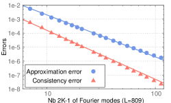
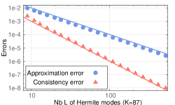
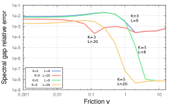
We expect the operator ΠM,0ΠM,0subscriptΠ𝑀0subscriptΠ𝑀0\Pi_{M,0}\mathcal{L}\Pi_{M,0} to be larger in a certain sense than ΠM,0(1ΠM,0)subscriptΠ𝑀01subscriptΠ𝑀0\Pi_{M,0}\mathcal{L}(1-\Pi_{M,0}) in L2(μ)superscriptL2𝜇{\mathrm{L}^{2}(\mu)}, so that (45) suggests that the consistency error is smaller than the approximation error (1ΠM)Φnorm1subscriptΠ𝑀Φ\|(1-\Pi_{M})\Phi\|. This is indeed what we observe in the numerical experiments we present in Figure 1. This shows that the way we bound the consistency error is probably not as sharp as it could be.

3.4 Matrix conditioning and linear systems

We introduce in this section the linear system associated with the practical implementation of either the Galerkin formulation (19) in the conformal case VML02(μ)subscript𝑉𝑀superscriptsubscriptL02𝜇V_{M}\subset{\mathrm{L}_{0}^{2}(\mu)}, or of (32) in the non-conformal case VML2(μ)subscript𝑉𝑀superscriptL2𝜇V_{M}\subset{\mathrm{L}^{2}(\mu)} but VML02(μ)not-subset-ofsubscript𝑉𝑀superscriptsubscriptL02𝜇V_{M}\not\subset{\mathrm{L}_{0}^{2}(\mu)}. In any case, we denote by (ej)1jMsubscriptsubscript𝑒𝑗1𝑗𝑀(e_{j})_{1\leqslant j\leqslant M} an orthogonal basis of the Galerkin space VMsubscript𝑉𝑀V_{M}, assumed to be of dimension M𝑀M.

Conformal case.

The weak formulation (19) can be equivalently reformulated as the linear system

𝐋M𝐗M=𝐘M,subscript𝐋𝑀subscript𝐗𝑀subscript𝐘𝑀\mathbf{L}_{M}\mathbf{X}_{M}=\mathbf{Y}_{M}, (49)

where

1i,jM,(𝐋M)i,j=ei,ej,(𝐗M)i=ΦM,ei,(𝐘M)i=R,ei.formulae-sequencefor-all1𝑖formulae-sequence𝑗𝑀formulae-sequencesubscriptsubscript𝐋𝑀𝑖𝑗subscript𝑒𝑖subscript𝑒𝑗formulae-sequencesubscriptsubscript𝐗𝑀𝑖subscriptΦ𝑀subscript𝑒𝑖subscriptsubscript𝐘𝑀𝑖𝑅subscript𝑒𝑖\forall 1\leqslant i,j\leqslant M,\qquad\left(\mathbf{L}_{M}\right)_{i,j}=\left\langle e_{i},-\mathcal{L}e_{j}\right\rangle,\quad\left(\mathbf{X}_{M}\right)_{i}=\left\langle\Phi_{M},e_{i}\right\rangle,\quad\left(\mathbf{Y}_{M}\right)_{i}=\left\langle R,e_{i}\right\rangle.

When the assumptions of Theorem 2 hold, (49) admits a unique solution, so that 𝐋Msubscript𝐋𝑀\mathbf{L}_{M} is invertible. Moreover 𝐋M1C/λγ,Mnormsuperscriptsubscript𝐋𝑀1𝐶subscript𝜆𝛾𝑀\|\mathbf{L}_{M}^{-1}\|\leqslant C/\lambda_{\gamma,M} is bounded uniformly in M𝑀M for MM0𝑀subscript𝑀0M\geqslant M_{0}. The linear system is therefore well-conditioned, and can be solved efficiently using any solver adapted to non-symmetric problems.

Non-conformal case.

We suppose that the assumptions of Corollary 3 hold. Let us introduce the vector 𝐔MMsubscript𝐔𝑀superscript𝑀\mathbf{U}_{M}\in\mathbb{R}^{M} corresponding to uMVMsubscript𝑢𝑀subscript𝑉𝑀u_{M}\in V_{M}:

1iM,(𝐔M)i=uM,ei=𝟏,eiΠM𝟏.formulae-sequencefor-all1𝑖𝑀subscriptsubscript𝐔𝑀𝑖subscript𝑢𝑀subscript𝑒𝑖1subscript𝑒𝑖normsubscriptΠ𝑀1\forall 1\leqslant i\leqslant M,\qquad\left(\mathbf{U}_{M}\right)_{i}=\left\langle u_{M},e_{i}\right\rangle=\frac{\left\langle\mathbf{1},e_{i}\right\rangle}{\|\Pi_{M}\mathbf{1}\|}.

Then the saddle-point problem (33) is equivalent to

{𝐋M𝐗M+λ𝐔M=𝐘M,𝐔M𝐗M=0,\left\{\begin{aligned} \mathbf{L}_{M}\mathbf{X}_{M}+\lambda\mathbf{U}_{M}&=\mathbf{Y}_{M},\\ \mathbf{U}_{M}^{\top}\mathbf{X}_{M}&=0,\end{aligned}\right.

with the same definition for 𝐋Msubscript𝐋𝑀\mathbf{L}_{M} and 𝐘Msubscript𝐘𝑀\mathbf{Y}_{M} as in the conformal case. With

𝐋^M=(𝐋M𝐔M𝐔M0),𝐗^M=(𝐗Mλ),𝐘^M=(𝐘M0),formulae-sequencesubscript^𝐋𝑀matrixmissing-subexpressionmissing-subexpressionmissing-subexpressionmissing-subexpressionmissing-subexpressionmissing-subexpressionsubscript𝐋𝑀missing-subexpressionmissing-subexpressionsubscript𝐔𝑀missing-subexpressionmissing-subexpressionmissing-subexpressionmissing-subexpressionmissing-subexpressionmissing-subexpressionmissing-subexpressionsuperscriptsubscript𝐔𝑀topmissing-subexpressionmissing-subexpression0formulae-sequencesubscript^𝐗𝑀matrixmissing-subexpressionsubscript𝐗𝑀missing-subexpressionmissing-subexpression𝜆subscript^𝐘𝑀matrixmissing-subexpressionsubscript𝐘𝑀missing-subexpressionmissing-subexpression0\widehat{\mathbf{L}}_{M}=\begin{pmatrix}&&&\vline&\\ &\mathbf{L}_{M}&&\vline&\mathbf{U}_{M}\\ &&&\vline&\\ \hline\cr&\displaystyle\phantom{\int}\mathbf{U}_{M}^{\top}&&\vline&0\end{pmatrix},\qquad\widehat{\mathbf{X}}_{M}=\begin{pmatrix}\\ \mathbf{X}_{M}\\ \\ \hline\cr\lambda\end{pmatrix},\qquad\widehat{\mathbf{Y}}_{M}=\begin{pmatrix}\\ \mathbf{Y}_{M}\\ \\ \hline\cr 0\end{pmatrix}, (50)

the saddle-point problem can finally be rewritten as

𝐋^M𝐗^M=𝐘^M.subscript^𝐋𝑀subscript^𝐗𝑀subscript^𝐘𝑀\widehat{\mathbf{L}}_{M}\widehat{\mathbf{X}}_{M}=\widehat{\mathbf{Y}}_{M}.

Proposition 2 and (40) imply that 𝐋^Msubscript^𝐋𝑀\widehat{\mathbf{L}}_{M} is invertible, with 𝐋^M1normsuperscriptsubscript^𝐋𝑀1\left\|\widehat{\mathbf{L}}_{M}^{-1}\right\| uniformly bounded in M𝑀M for MM0𝑀subscript𝑀0M\geqslant M_{0}. This proves that the matrix 𝐋^Msubscript^𝐋𝑀\widehat{\mathbf{L}}_{M} does not have vanishing eigenvalues, in contrast to 𝐋Msubscript𝐋𝑀\mathbf{L}_{M} (since 𝐋M𝐔MM0𝑀absentsubscript𝐋𝑀subscript𝐔𝑀0\mathbf{L}_{M}\mathbf{U}_{M}\xrightarrow[M\to\infty]{}0). Therefore the linear system 𝐋^M𝐗^M=𝐘^Msubscript^𝐋𝑀subscript^𝐗𝑀subscript^𝐘𝑀\widehat{\mathbf{L}}_{M}\widehat{\mathbf{X}}_{M}=\widehat{\mathbf{Y}}_{M} can be solved as efficiently as in the conformal case. In the following we choose to use a sparse LU factorization.

Remark 4.

Let us conclude this section with some criteria discriminating a good Galerkin space, and more generally a good function basis. Anticipating on the analysis of Section 4.1, a standard choice is to use tensorized bases. The difficult part is to find a basis to describe the position dependence of the function of consideration. This requires considering the following points:

  • approximation errors and consistency errors should be small. It should be checked in particular that condition (21) holds and that the norm of the operator ΠM(1ΠM)subscriptΠ𝑀1subscriptΠ𝑀\Pi_{M}\mathcal{L}(1-\Pi_{M}) does not grow too fast.

  • the implementation is easier if the space is conformal, since it avoids the computation of 𝐔Msubscript𝐔𝑀\mathbf{U}_{M} using integral quadratures.

  • when the basis is non-orthogonal, the Gram matrix should be inverted. The latter can be ill conditioned, leading to numerically instability, specifically for unbounded position spaces.

4 Application to a simple one-dimensional system

We present in this section an application of the theory developed in Section 3 to a specific example, described in Section 4.1 together with the Galerkin basis used to discretize the generator. This allows us to prove explicit convergence rates for the approximation error (Section 4.2) and the consistency error (Section 4.3). For the latter error, we have to further specify the potential in order to check the assumptions ensuring the hypocoercivity of the discretized generator. The final, global error estimate is summarized in (61). The technical proofs of some claims and bounds are postponed to Appendix B. We finally present in Section 4.4 some numerical results illustrating the predicted error bounds.

4.1 Description of the system and the Galerkin space

We consider a single particle in a one-dimensional periodic potential: D=1𝐷1D=1, m=1𝑚1m=1 and 𝒟=2π𝕋=/2π𝒟2𝜋𝕋2𝜋\mathcal{D}=2\pi\mathbb{T}=\mathbb{R}/2\pi\mathbb{Z}. The Galerkin space is constructed using the spectral tensor basis

ek,(q,p)=Gk(q)H(p),subscript𝑒𝑘𝑞𝑝subscript𝐺𝑘𝑞subscript𝐻𝑝e_{k,\ell}(q,p)=G_{k}(q)H_{\ell}(p),

where 0k<2K10𝑘2𝐾10\leqslant k<2K-1 and 0<L0𝐿0\leqslant\ell<L. Compared to the notation of Section 3, the basis size M=(2K1)L𝑀2𝐾1𝐿M=(2K-1)L depends on two parameters K,L𝐾𝐿K,L, which both have to go to infinity for the convergence results to hold. In this section we prefer the index KL𝐾𝐿KL instead of M𝑀M, denoting thus VKLsubscript𝑉𝐾𝐿V_{KL}, ΠKLsubscriptΠ𝐾𝐿\Pi_{KL}, ΦKLsubscriptΦ𝐾𝐿\Phi_{KL},… In the remainder of this section we describe our choices for Gksubscript𝐺𝑘G_{k} and Hsubscript𝐻H_{\ell}.

Note that the size of the matrix, namely the number of tensorized basis elements, increases exponentially with the dimension of the system. In larger dimension one could consider resorting to tensor formats [13], as is done for the high-dimensional Schrödinger equation in [34], carefully making use of the symmetries and of the structure of the equation.

Weighted Fourier basis (Gk)subscript𝐺𝑘(G_{k}).

Fourier modes provide a natural basis to approximate periodic functions, such as functions of the positions here. Since the measure appearing in the scalar product is ν𝜈\nu, we consider in fact the following L2(ν)superscript𝐿2𝜈L^{2}(\nu)-orthonormal modes:

G0(q)subscript𝐺0𝑞\displaystyle G_{0}(q) =Zβ,ν2πeβV(q)/2,absentsubscript𝑍𝛽𝜈2𝜋superscripte𝛽𝑉𝑞2\displaystyle=\sqrt{\frac{Z_{\beta,\nu}}{2\pi}}\,\mathrm{e}^{\beta V(q)/2}, (51)
G2k(q)subscript𝐺2𝑘𝑞\displaystyle G_{2k}(q) =Zβ,νπcos(kq)eβV(q)/2,k1,formulae-sequenceabsentsubscript𝑍𝛽𝜈𝜋𝑘𝑞superscripte𝛽𝑉𝑞2𝑘1\displaystyle=\sqrt{\frac{Z_{\beta,\nu}}{\pi}}\cos(kq)\,\mathrm{e}^{\beta V(q)/2},\qquad k\geqslant 1,
G2k1(q)subscript𝐺2𝑘1𝑞\displaystyle G_{2k-1}(q) =Zβ,νπsin(kq)eβV(q)/2,k1.formulae-sequenceabsentsubscript𝑍𝛽𝜈𝜋𝑘𝑞superscripte𝛽𝑉𝑞2𝑘1\displaystyle=\sqrt{\frac{Z_{\beta,\nu}}{\pi}}\sin(kq)\,\mathrm{e}^{\beta V(q)/2},\qquad k\geqslant 1.

Note that the functions Gksubscript𝐺𝑘G_{k} for k1𝑘1k\geqslant 1 do not have mean 0 with respect to ν𝜈\nu (except for very specific potentials such as V=0𝑉0V=0). The spanned discretization space is thus non-conformal: VKLL02(μ)not-subset-ofsubscript𝑉𝐾𝐿superscriptsubscriptL02𝜇V_{KL}\not\subset{\mathrm{L}_{0}^{2}(\mu)}.

Hermite functions basis (H)subscript𝐻(H_{\ell}).

Since the marginal measure κ𝜅\kappa in the momentum variables is Gaussian with variance β1superscript𝛽1\beta^{-1}, we consider the following orthonormal Hermite modes for \ell\in\mathbb{N}:

H(p)=1!H~(βp),H~(y)=(1)ey22ddy(ey22).formulae-sequencesubscript𝐻𝑝1subscript~𝐻𝛽𝑝subscript~𝐻𝑦superscript1superscriptesuperscript𝑦22superscript𝑑𝑑superscript𝑦superscriptesuperscript𝑦22H_{\ell}(p)=\frac{1}{\sqrt{\ell!}}\widetilde{H}_{\ell}\left(\sqrt{\beta}p\right),\qquad\widetilde{H}_{\ell}(y)=(-1)^{\ell}\mathrm{e}^{\frac{y^{2}}{2}}\frac{d^{\ell}}{dy^{\ell}}\left(\mathrm{e}^{-\frac{y^{2}}{2}}\right).

They are well suited to our problem since they are the eigenfunctions of the symmetric part FD=β1ppsubscriptFDsuperscript𝛽1superscriptsubscript𝑝subscript𝑝{\mathcal{L}_{\mathrm{FD}}}=-\beta^{-1}\partial_{p}^{*}\partial_{p} of the generator. Indeed,

,pH=βH1andpH=β(+1)H+1,formulae-sequencefor-allformulae-sequencesubscript𝑝subscript𝐻𝛽subscript𝐻1andsuperscriptsubscript𝑝subscript𝐻𝛽1subscript𝐻1\forall\ell\in\mathbb{N},\qquad\partial_{p}H_{\ell}=\sqrt{\beta\ell}H_{\ell-1}\qquad\mbox{and}\quad\partial_{p}^{*}H_{\ell}=\sqrt{\beta(\ell+1)}H_{\ell+1}, (52)

so that

,FDH=H.formulae-sequencefor-allsubscriptFDsubscript𝐻subscript𝐻\forall\ell\in\mathbb{N},\qquad{\mathcal{L}_{\mathrm{FD}}}H_{\ell}=-\ell H_{\ell}. (53)
Remark 5.

The basis we consider is similar to the one used in [29] and [24], where the modes in position are the standard Fourier modes. The latter modes are orthogonal for the uniform measure on the compact position space 𝒟𝒟\mathcal{D} rather than on L2(ν)superscriptL2𝜈{\mathrm{L}^{2}(\nu)}. Therefore, the scalar product used in Subsection 3.4 should be replaced with the scalar product associated with the measure μ~(dqdp)=|𝒟|1κ(dp)dq~𝜇𝑞𝑝superscript𝒟1𝜅𝑝𝑞\widetilde{\mu}(\differential q\,\differential p)=|\mathcal{D}|^{-1}\kappa(\differential p)\,\differential q. The results of Section 3 could be adapted to this scalar product since the measures μ𝜇\mu and μ~~𝜇\widetilde{\mu} are equivalent. Note that the discretization based on the standard Fourier modes is a conformal one since one of the tensorized modes is proportional to 𝟏1\mathbf{1}, which simplifies the implementation. It is however not generalizable to unbounded position spaces because the uniform measure is not normalizable. An interesting question, not considered in this work, is to quantify the relative performances of the approaches based on orthonormal bases either on L2(μ)superscriptL2𝜇{\mathrm{L}^{2}(\mu)} or L2(μ~)superscriptL2~𝜇\mathrm{L}^{2}(\widetilde{\mu}).

Rigidity matrix.

In order to give the expression of the rigidity matrix, we introduce, for a Fourier basis of 2K12𝐾12K-1 weighted Fourier modes, the matrix 𝐐𝐐\mathbf{Q} with entries

𝐐k,k=Gk,qGkL2(ν),subscript𝐐𝑘superscript𝑘subscriptsubscript𝐺𝑘subscript𝑞subscript𝐺superscript𝑘superscriptL2𝜈\mathbf{Q}_{k,k^{\prime}}=\left\langle G_{k},\partial_{q}G_{k^{\prime}}\right\rangle_{\mathrm{L}^{2}(\nu)}, (54)

and, for L𝐿L Hermite modes, the matrix 𝐏𝐏\mathbf{P} with entries

𝐏,=H,pHL2(κ)=H,βH1L2(κ)=βδ,1.subscript𝐏superscriptsubscriptsubscript𝐻subscript𝑝subscript𝐻superscriptsuperscriptL2𝜅subscriptsubscript𝐻𝛽superscriptsubscript𝐻superscript1superscriptL2𝜅𝛽superscriptsubscript𝛿superscript1\mathbf{P}_{\ell,\ell^{\prime}}=\left\langle H_{\ell},\partial_{p}H_{\ell^{\prime}}\right\rangle_{\mathrm{L}^{2}(\kappa)}=\left\langle H_{\ell},\sqrt{\beta\ell^{\prime}}H_{\ell^{\prime}-1}\right\rangle_{\mathrm{L}^{2}(\kappa)}=\sqrt{\beta\ell^{\prime}}\delta_{\ell,\ell^{\prime}-1}. (55)

Note that 𝐏𝐏\mathbf{P} is sparse in view of (52). The matrix 𝐐𝐐\mathbf{Q} is, on the other hand, dense in general, except when V𝑉V is a trigonometric polynomial. In the following, we choose V(q)=1cos(q)𝑉𝑞1𝑞V(q)=1-\cos(q) in order for 𝐐𝐐\mathbf{Q} to be tridiagonal. For a general, smooth potential V𝑉V, 𝐐𝐐\mathbf{Q} would be dense but with coefficients which decay fast away from the diagonal.

The rigidity matrix which appears on the left-hand side of (49) has entries (for 0k2K20𝑘2𝐾20\leqslant k\leqslant 2K-2 and 0L10𝐿10\leqslant\ell\leqslant L-1)

𝐋k,ksubscript𝐋𝑘superscript𝑘superscript\displaystyle\mathbf{L}_{k\ell,k^{\prime}\ell^{\prime}} =ek,ekabsentsubscript𝑒𝑘subscript𝑒superscript𝑘superscript\displaystyle=\left\langle e_{k\ell},-\mathcal{L}e_{k^{\prime}\ell^{\prime}}\right\rangle
=β1[GkH,qpGkHGkH,qpGkHγGkH,ppGkH]absentsuperscript𝛽1delimited-[]subscript𝐺𝑘subscript𝐻subscript𝑞superscriptsubscript𝑝subscript𝐺superscript𝑘subscript𝐻superscriptsubscript𝐺𝑘subscript𝐻superscriptsubscript𝑞subscript𝑝subscript𝐺superscript𝑘subscript𝐻superscript𝛾subscript𝐺𝑘subscript𝐻superscriptsubscript𝑝subscript𝑝subscript𝐺superscript𝑘subscript𝐻superscript\displaystyle=-\beta^{-1}\left[\left\langle G_{k}H_{\ell},\partial_{q}\partial_{p}^{*}G_{k^{\prime}}H_{\ell^{\prime}}\right\rangle-\left\langle G_{k}H_{\ell},\partial_{q}^{*}\partial_{p}G_{k^{\prime}}H_{\ell^{\prime}}\right\rangle-\gamma\left\langle G_{k}H_{\ell},\partial_{p}^{*}\partial_{p}G_{k^{\prime}}H_{\ell^{\prime}}\right\rangle\right]
=β1𝐐k,k𝐏,+β1𝐐k,k𝐏,+γ𝐈k,k𝐍,,absentsuperscript𝛽1subscript𝐐𝑘superscript𝑘subscript𝐏superscriptsuperscript𝛽1subscript𝐐superscript𝑘𝑘subscript𝐏superscript𝛾subscript𝐈𝑘superscript𝑘subscript𝐍superscript\displaystyle=-\beta^{-1}\mathbf{Q}_{k,k^{\prime}}\mathbf{P}_{\ell^{\prime},\ell}+\beta^{-1}\mathbf{Q}_{k^{\prime},k}\mathbf{P}_{\ell,\ell^{\prime}}+\gamma\mathbf{I}_{k,k^{\prime}}\mathbf{N}_{\ell,\ell^{\prime}},

where 𝐈k,k=δk,ksubscript𝐈𝑘superscript𝑘subscript𝛿𝑘superscript𝑘\mathbf{I}_{k,k^{\prime}}=\delta_{k,k^{\prime}} and 𝐍,=δ,subscript𝐍superscriptsubscript𝛿superscript\mathbf{N}_{\ell,\ell^{\prime}}=\ell\,\delta_{\ell,\ell^{\prime}}. In practice we transform these tensors into matrices by a hashing function ζ:(k,)ζ(k,):𝜁𝑘𝜁𝑘\zeta:(k,\ell)\to\zeta(k,\ell)\in\mathbb{N}. The matrix 𝐋𝐋\mathbf{L} is then of size (2K1)L2𝐾1𝐿(2K-1)L.

4.2 Approximation error for the tensor basis

We define the projectors ΠKqsuperscriptsubscriptΠ𝐾𝑞\Pi_{K}^{q} and ΠLpsuperscriptsubscriptΠ𝐿𝑝\Pi_{L}^{p} by

ΠKqφ=k=02K2φ,GkGk,ΠLpφ==0L1φ,HH.formulae-sequencesuperscriptsubscriptΠ𝐾𝑞𝜑superscriptsubscript𝑘02𝐾2𝜑subscript𝐺𝑘subscript𝐺𝑘superscriptsubscriptΠ𝐿𝑝𝜑superscriptsubscript0𝐿1𝜑subscript𝐻subscript𝐻\Pi_{K}^{q}\varphi=\sum_{k=0}^{2K-2}\left\langle\varphi,G_{k}\right\rangle G_{k},\qquad\Pi_{L}^{p}\varphi=\sum_{\ell=0}^{L-1}\left\langle\varphi,H_{\ell}\right\rangle H_{\ell}.

Their complements are ΠKq=1ΠKqsuperscriptsubscriptΠ𝐾perpendicular-to𝑞absent1superscriptsubscriptΠ𝐾𝑞\Pi_{K}^{q\perp}=1-\Pi_{K}^{q} and ΠLp=1ΠLpsuperscriptsubscriptΠ𝐿perpendicular-to𝑝absent1superscriptsubscriptΠ𝐿𝑝\Pi_{L}^{p\perp}=1-\Pi_{L}^{p}. With this notation, the projector onto the Galerkin space is ΠKL=ΠKqΠLpsubscriptΠ𝐾𝐿superscriptsubscriptΠ𝐾𝑞superscriptsubscriptΠ𝐿𝑝\Pi_{KL}=\Pi_{K}^{q}\Pi_{L}^{p}. The study of the approximation error (1ΠKL)Φ1subscriptΠ𝐾𝐿Φ(1-\Pi_{KL})\Phi is performed by first estimating the error arising from the projection ΠKqsuperscriptsubscriptΠ𝐾𝑞\Pi_{K}^{q} (see Lemma 2), and then the error arising from ΠLpsuperscriptsubscriptΠ𝐿𝑝\Pi_{L}^{p} (see Lemma 3). The conclusion follows by remarking that

01ΠKL=1ΠKq+ΠKq(1ΠLp)ΠKq+ΠLp,01subscriptΠ𝐾𝐿1superscriptsubscriptΠ𝐾𝑞superscriptsubscriptΠ𝐾𝑞1superscriptsubscriptΠ𝐿𝑝superscriptsubscriptΠ𝐾perpendicular-to𝑞absentsuperscriptsubscriptΠ𝐿perpendicular-to𝑝absent0\leqslant 1-\Pi_{KL}=1-\Pi_{K}^{q}+\Pi_{K}^{q}(1-\Pi_{L}^{p})\leqslant\Pi_{K}^{q\perp}+\Pi_{L}^{p\perp}, (56)

see Proposition 3.

Lemma 2.

Assume that V𝑉V is smooth. Then, for any s𝑠s\in\mathbb{N}, there exists Ms+subscript𝑀𝑠subscriptM_{s}\in\mathbb{R}_{+} such that

φHs(ν),K1,φΠKqφL2(ν)MsKsφHs(ν).formulae-sequencefor-all𝜑superscriptH𝑠𝜈formulae-sequencefor-all𝐾1subscriptnorm𝜑superscriptsubscriptΠ𝐾𝑞𝜑superscriptL2𝜈subscript𝑀𝑠superscript𝐾𝑠subscriptnorm𝜑superscriptH𝑠𝜈\forall\varphi\in\mathrm{H}^{s}(\nu),\quad\forall K\geqslant 1,\qquad\left\|\varphi-\Pi_{K}^{q}\varphi\right\|_{\mathrm{L}^{2}(\nu)}\leqslant\frac{M_{s}}{K^{s}}\|\varphi\|_{\mathrm{H}^{s}(\nu)}.
Proof.

For φHs(ν)𝜑superscriptH𝑠𝜈\varphi\in\mathrm{H}^{s}(\nu), we introduce φ~=Zβ,ν1/2eβV/2φL2(dq)~𝜑superscriptsubscript𝑍𝛽𝜈12superscripte𝛽𝑉2𝜑superscriptL2𝑞\widetilde{\varphi}=Z_{\beta,\nu}^{-1/2}\mathrm{e}^{-\beta V/2}\varphi\in\mathrm{L}^{2}(\differential q), as well as the flat Fourier basis G~k=Zβ,ν1/2eβV/2Gksubscript~𝐺𝑘superscriptsubscript𝑍𝛽𝜈12superscripte𝛽𝑉2subscript𝐺𝑘\widetilde{G}_{k}=Z_{\beta,\nu}^{-1/2}\mathrm{e}^{-\beta V/2}G_{k} which is orthonormal on L2([0,2π])superscriptL202𝜋\mathrm{L}^{2}([0,2\pi]). Since 𝒟=2π𝕋𝒟2𝜋𝕋\mathcal{D}=2\pi\mathbb{T} is compact, Hs(ν)=Hs(dq)superscriptH𝑠𝜈superscriptH𝑠𝑞\mathrm{H}^{s}(\nu)=\mathrm{H}^{s}(\differential q) for any s𝑠s\in\mathbb{N} and there exists Ms+subscript𝑀𝑠subscriptM_{s}\in\mathbb{R}_{+} such that

qsφL2(dq)MsφHs(ν).subscriptnormsuperscriptsubscript𝑞𝑠𝜑superscriptL2𝑞subscript𝑀𝑠subscriptnorm𝜑superscriptH𝑠𝜈\|\partial_{q}^{s}\varphi\|_{\mathrm{L}^{2}(\differential q)}\leqslant M_{s}\|\varphi\|_{\mathrm{H}^{s}(\nu)}. (57)

By the Bessel-Parseval inequality,

φΠKqφL2(ν)2superscriptsubscriptnorm𝜑superscriptsubscriptΠ𝐾𝑞𝜑superscriptL2𝜈2\displaystyle\|\varphi-\Pi_{K}^{q}\varphi\|_{\mathrm{L}^{2}(\nu)}^{2} =k2K1φ,Gk2=k2K1(02πφ~G~kdq)2absentsubscript𝑘2𝐾1superscript𝜑subscript𝐺𝑘2subscript𝑘2𝐾1superscriptsuperscriptsubscript02𝜋~𝜑subscript~𝐺𝑘𝑞2\displaystyle=\sum_{k\geqslant 2K-1}\left\langle\varphi,G_{k}\right\rangle^{2}=\sum_{k\geqslant 2K-1}\left(\int_{0}^{2\pi}\widetilde{\varphi}\,\widetilde{G}_{k}\,\differential q\right)^{2}
=1πkK(02πφ~(q)cos(kq)dq)2+(02πφ~(q)sin(kq)dq)2absent1𝜋subscript𝑘𝐾superscriptsuperscriptsubscript02𝜋~𝜑𝑞𝑘𝑞𝑞2superscriptsuperscriptsubscript02𝜋~𝜑𝑞𝑘𝑞𝑞2\displaystyle=\frac{1}{\pi}\sum_{k\geqslant K}\left(\int_{0}^{2\pi}\widetilde{\varphi}(q)\,\cos(kq)\,\differential q\right)^{2}+\left(\int_{0}^{2\pi}\widetilde{\varphi}(q)\,\sin(kq)\,\differential q\right)^{2}
1πkK(02πφ~(q)ksKscos(kq)dq)2+(02πφ~(q)ksKssin(kq)dq)2absent1𝜋subscript𝑘𝐾superscriptsuperscriptsubscript02𝜋~𝜑𝑞superscript𝑘𝑠superscript𝐾𝑠𝑘𝑞𝑞2superscriptsuperscriptsubscript02𝜋~𝜑𝑞superscript𝑘𝑠superscript𝐾𝑠𝑘𝑞𝑞2\displaystyle\leqslant\frac{1}{\pi}\sum_{k\geqslant K}\left(\int_{0}^{2\pi}\widetilde{\varphi}(q)\,\frac{k^{s}}{K^{s}}\cos(kq)\,\differential q\right)^{2}+\left(\int_{0}^{2\pi}\widetilde{\varphi}(q)\,\frac{k^{s}}{K^{s}}\sin(kq)\,\differential q\right)^{2}
=1πK2skK(02πφ~(q)qscos(kq)dq)2+(02πφ~(q)qssin(kq)dq)2absent1𝜋superscript𝐾2𝑠subscript𝑘𝐾superscriptsuperscriptsubscript02𝜋~𝜑𝑞superscriptsubscript𝑞𝑠𝑘𝑞𝑞2superscriptsuperscriptsubscript02𝜋~𝜑𝑞superscriptsubscript𝑞𝑠𝑘𝑞𝑞2\displaystyle=\frac{1}{\pi K^{2s}}\sum_{k\geqslant K}\left(\int_{0}^{2\pi}\widetilde{\varphi}(q)\,\partial_{q}^{s}\cos(kq)\,\differential q\right)^{2}+\left(\int_{0}^{2\pi}\widetilde{\varphi}(q)\,\partial_{q}^{s}\sin(kq)\,\differential q\right)^{2}
1K2sqsφ~L2(dq)2,absent1superscript𝐾2𝑠superscriptsubscriptnormsuperscriptsubscript𝑞𝑠~𝜑superscriptL2𝑞2\displaystyle\leqslant\frac{1}{K^{2s}}\|\partial_{q}^{s}\widetilde{\varphi}\|_{\mathrm{L}^{2}(\differential q)}^{2},

which allows to conclude with (57). ∎

Lemma 3.

For any s𝑠s\in\mathbb{N} and φHs(κ)𝜑superscriptH𝑠𝜅\varphi\in\mathrm{H}^{s}(\kappa), it holds

Ls,φΠLpφL2(κ)[β(Ls+1)]s/2psφL2(κ).formulae-sequencefor-all𝐿𝑠subscriptnorm𝜑superscriptsubscriptΠ𝐿𝑝𝜑superscriptL2𝜅superscriptdelimited-[]𝛽𝐿𝑠1𝑠2subscriptnormsuperscriptsubscript𝑝𝑠𝜑superscriptL2𝜅\forall L\geqslant s,\qquad\left\|\varphi-\Pi_{L}^{p}\varphi\right\|_{\mathrm{L}^{2}(\kappa)}\leqslant\left[\beta(L-s+1)\right]^{-s/2}\|\partial_{p}^{s}\varphi\|_{\mathrm{L}^{2}(\kappa)}.
Proof.

Fix Ls𝐿𝑠L\geqslant s. In view of (52), it holds

(p)sHs=βs/2(s+1)H,superscriptsuperscriptsubscript𝑝𝑠subscript𝐻𝑠superscript𝛽𝑠2𝑠1subscript𝐻\left(\partial_{p}^{*}\right)^{s}H_{\ell-s}=\beta^{s/2}\sqrt{(\ell-s+1)\dots\ell}\,H_{\ell},

with (s+1)(Ls+1)s/2𝑠1superscript𝐿𝑠1𝑠2\sqrt{(\ell-s+1)\dots\ell}\geqslant(L-s+1)^{s/2} when L𝐿\ell\geqslant L. Therefore,

φΠLpφL2(κ)2=Lφ,H2superscriptsubscriptnorm𝜑superscriptsubscriptΠ𝐿𝑝𝜑superscriptL2𝜅2subscript𝐿superscript𝜑subscript𝐻2\displaystyle\|\varphi-\Pi_{L}^{p}\varphi\|_{\mathrm{L}^{2}(\kappa)}^{2}=\sum_{\ell\geqslant L}\left\langle\varphi,H_{\ell}\right\rangle^{2} Lφ,(s+1)(Ls+1)s/2H2absentsubscript𝐿superscript𝜑𝑠1superscript𝐿𝑠1𝑠2subscript𝐻2\displaystyle\leqslant\sum_{\ell\geqslant L}\left\langle\varphi,\frac{\sqrt{(\ell-s+1)\dots\ell}}{(L-s+1)^{\nicefrac{{s}}{{2}}}}H_{\ell}\right\rangle^{2}
=[β(Ls+1)]sLφ,(p)sHs2absentsuperscriptdelimited-[]𝛽𝐿𝑠1𝑠subscript𝐿superscript𝜑superscriptsuperscriptsubscript𝑝𝑠subscript𝐻𝑠2\displaystyle=\left[\beta(L-s+1)\right]^{-s}\sum_{\ell\geqslant L}\left\langle\varphi,(\partial_{p}^{*})^{s}H_{\ell-s}\right\rangle^{2}
[β(Ls+1)]spsφL2(κ)2,absentsuperscriptdelimited-[]𝛽𝐿𝑠1𝑠superscriptsubscriptnormsuperscriptsubscript𝑝𝑠𝜑superscriptL2𝜅2\displaystyle\leqslant\left[\beta(L-s+1)\right]^{-s}\|\partial_{p}^{s}\varphi\|_{\mathrm{L}^{2}(\kappa)}^{2},

from which the conclusion follows. ∎

The following approximation result is then directly deduced from the previous lemmas and (56).

Proposition 3.

Assume that V𝑉V is smooth. Then, for any s𝑠s\in\mathbb{N}, there exists As+subscript𝐴𝑠subscriptA_{s}\in\mathbb{R}_{+} such that

φHs(μ),K1,Ls,φΠKLφL2(μ)As(1Ks+1Ls/2)φHs(μ).formulae-sequencefor-all𝜑superscriptH𝑠𝜇formulae-sequencefor-all𝐾1formulae-sequence𝐿𝑠subscriptnorm𝜑subscriptΠ𝐾𝐿𝜑superscriptL2𝜇subscript𝐴𝑠1superscript𝐾𝑠1superscript𝐿𝑠2subscriptnorm𝜑superscriptH𝑠𝜇\forall\varphi\in{\mathrm{H}^{s}(\mu)},\qquad\forall K\geqslant 1,\ L\geqslant s,\qquad\|\varphi-\Pi_{KL}\varphi\|_{\mathrm{L}^{2}(\mu)}\leqslant A_{s}\left(\frac{1}{K^{s}}+\frac{1}{L^{s/2}}\right)\|\varphi\|_{{\mathrm{H}^{s}(\mu)}}.

The approximation error (1ΠKL)Φnorm1subscriptΠ𝐾𝐿Φ\|(1-\Pi_{KL})\Phi\| thus depends on the regularity of the solution ΦΦ\Phi of the Poisson problem. Now, the operator 1superscript1\mathcal{L}^{-1} is a bounded operator on Hs(μ)L02(μ)superscriptH𝑠𝜇superscriptsubscriptL02𝜇\mathrm{H}^{s}(\mu)\cap{\mathrm{L}_{0}^{2}(\mu)} for any s0𝑠0s\geqslant 0 by the results of [31, Section 3.2] and [18] (see also [9, 16]). Therefore, when RHs(μ)L02(μ)𝑅superscriptH𝑠𝜇superscriptsubscriptL02𝜇R\in\mathrm{H}^{s}(\mu)\cap{\mathrm{L}_{0}^{2}(\mu)}, the solution ΦΦ\Phi belongs to Hs(μ)L02(μ)superscriptH𝑠𝜇superscriptsubscriptL02𝜇\mathrm{H}^{s}(\mu)\cap{\mathrm{L}_{0}^{2}(\mu)}, and there is A~s+subscript~𝐴𝑠subscript\widetilde{A}_{s}\in\mathbb{R}_{+} such that

ΦΠKLΦL2(μ)ΦΠKqΦL2(μ)+ΦΠLpΦL2(μ)A~s(1Ks+1Ls/2)RHs(μ).subscriptnormΦsubscriptΠ𝐾𝐿ΦsuperscriptL2𝜇subscriptnormΦsuperscriptsubscriptΠ𝐾𝑞ΦsuperscriptL2𝜇subscriptnormΦsuperscriptsubscriptΠ𝐿𝑝ΦsuperscriptL2𝜇subscript~𝐴𝑠1superscript𝐾𝑠1superscript𝐿𝑠2subscriptnorm𝑅superscriptH𝑠𝜇\|\Phi-\Pi_{KL}\Phi\|_{\mathrm{L}^{2}(\mu)}\leqslant\|\Phi-\Pi_{K}^{q}\Phi\|_{\mathrm{L}^{2}(\mu)}+\|\Phi-\Pi_{L}^{p}\Phi\|_{\mathrm{L}^{2}(\mu)}\leqslant\widetilde{A}_{s}\left(\frac{1}{K^{s}}+\frac{1}{L^{s/2}}\right)\|R\|_{{\mathrm{H}^{s}(\mu)}}. (58)
Remark 6.

In fact, it can be expected that the operator 1superscript1\mathcal{L}^{-1} further regularizes in the momentum variable; more precisely that pΦHs(μ)subscript𝑝ΦsuperscriptH𝑠𝜇\partial_{p}\Phi\in\mathrm{H}^{s}(\mu) when RHs(μ)𝑅superscriptH𝑠𝜇R\in\mathrm{H}^{s}(\mu). This is consistent with what we observe in the numerical simulations reported in Section 4.4. Note also that the estimates provided by [31, 9, 16, 18] are obtained for a fixed friction γ>0𝛾0\gamma>0. Some additional work is needed to carefully quantify their dependence upon γ𝛾\gamma, although we expect that the bounds on 1superscript1\mathcal{L}^{-1} considered as an operator on Hs(μ)L02(μ)superscriptH𝑠𝜇superscriptsubscriptL02𝜇\mathrm{H}^{s}(\mu)\cap{\mathrm{L}_{0}^{2}(\mu)} should still scale as max(γ,γ1)𝛾superscript𝛾1\max(\gamma,\gamma^{-1}).

Let us conclude this section by an approximation result involving ΠKL,0subscriptΠ𝐾𝐿0\Pi_{KL,0} rather than ΠKLsubscriptΠ𝐾𝐿\Pi_{KL} (see the decomposition (41), to be compared with (20)).

Corollary 4.

Assume that V𝑉V is smooth. Then, for any s𝑠s\in\mathbb{N}, there exists As+subscript𝐴𝑠subscriptA_{s}\in\mathbb{R}_{+} such that

φHs(μ)L02(μ),K1,Ls,φΠKL,0φL2(μ)As(1Ks+1Ls/2)φHs(μ).formulae-sequencefor-all𝜑superscriptH𝑠𝜇superscriptsubscriptL02𝜇formulae-sequencefor-all𝐾1formulae-sequence𝐿𝑠subscriptnorm𝜑subscriptΠ𝐾𝐿0𝜑superscriptL2𝜇subscript𝐴𝑠1superscript𝐾𝑠1superscript𝐿𝑠2subscriptnorm𝜑superscriptH𝑠𝜇\forall\varphi\in{\mathrm{H}^{s}(\mu)}\cap{\mathrm{L}_{0}^{2}(\mu)},\qquad\forall K\geqslant 1,\ L\geqslant s,\qquad\|\varphi-\Pi_{KL,0}\varphi\|_{\mathrm{L}^{2}(\mu)}\leqslant A_{s}\left(\frac{1}{K^{s}}+\frac{1}{L^{s/2}}\right)\|\varphi\|_{{\mathrm{H}^{s}(\mu)}}.
Proof.

Note first that H,𝟏=δ,0subscript𝐻1subscript𝛿0\left\langle H_{\ell},\mathbf{1}\right\rangle=\delta_{\ell,0}, so that ΠKL𝟏=ΠKq𝟏subscriptΠ𝐾𝐿1superscriptsubscriptΠ𝐾𝑞1\Pi_{KL}\mathbf{1}=\Pi_{K}^{q}\mathbf{1} and uK=ΠKq𝟏/ΠKq𝟏subscript𝑢𝐾superscriptsubscriptΠ𝐾𝑞1normsuperscriptsubscriptΠ𝐾𝑞1u_{K}=\Pi_{K}^{q}\mathbf{1}/\|\Pi_{K}^{q}\mathbf{1}\| depends only on the position variables for L1𝐿1L\geqslant 1. Next, in view of the computations performed in the proof of Corollary 3,

ΠKL,0φ=ΠKLφΠKq𝟏ΠKq𝟏,φuK,subscriptΠ𝐾𝐿0𝜑subscriptΠ𝐾𝐿𝜑superscriptsubscriptΠ𝐾𝑞1normsuperscriptsubscriptΠ𝐾𝑞1𝜑subscript𝑢𝐾\Pi_{KL,0}\varphi=\Pi_{KL}\varphi-\left\langle\frac{\Pi_{K}^{q}\mathbf{1}}{\|\Pi_{K}^{q}\mathbf{1}\|},\varphi\right\rangle u_{K},

where uK=1normsubscript𝑢𝐾1\|u_{K}\|=1. Since φL02(μ)𝜑superscriptsubscriptL02𝜇\varphi\in{\mathrm{L}_{0}^{2}(\mu)}, it holds in fact

ΠKq𝟏ΠKq𝟏,φ=(1ΠKq)𝟏ΠKq𝟏,φ,superscriptsubscriptΠ𝐾𝑞1normsuperscriptsubscriptΠ𝐾𝑞1𝜑1superscriptsubscriptΠ𝐾𝑞1normsuperscriptsubscriptΠ𝐾𝑞1𝜑\left\langle\frac{\Pi_{K}^{q}\mathbf{1}}{\|\Pi_{K}^{q}\mathbf{1}\|},\varphi\right\rangle=\left\langle\frac{(1-\Pi_{K}^{q})\mathbf{1}}{\|\Pi_{K}^{q}\mathbf{1}\|},\varphi\right\rangle,

which converges to 0 faster than any polynomial in K𝐾K in view of Proposition 3. ∎

4.3 Consistency error

In order to simplify the computations (in particular to have some simple structure on the derivatives of the Fourier modes) we consider the following potential:

V(q)=1cos(q).𝑉𝑞1𝑞V(q)=1-\cos(q).

In this case, using the trigonometric identities

2cos(kq)sin(q)2𝑘𝑞𝑞\displaystyle 2\cos(kq)\sin(q) =sin((k+1)q)sin((k1)q)absent𝑘1𝑞𝑘1𝑞\displaystyle=\sin((k+1)q)-\sin((k-1)q)
2sin(kq)sin(q)2𝑘𝑞𝑞\displaystyle 2\sin(kq)\sin(q) =cos((k+1)q)+cos((k1)q),absent𝑘1𝑞𝑘1𝑞\displaystyle=-\cos((k+1)q)+\cos((k-1)q),

a straightforward computation shows that the derivatives of the basis functions satisfy

qG0=β22G1,qG1=β22G0+G2β4G4,qG2k=β4G2k3kG2k1+β4G2k+1,qG2k1=β4G2k2+kG2kβ4G2k+2,subscript𝑞subscript𝐺0absent𝛽22subscript𝐺1subscript𝑞subscript𝐺1absent𝛽22subscript𝐺0subscript𝐺2𝛽4subscript𝐺4subscript𝑞subscript𝐺2𝑘absent𝛽4subscript𝐺2𝑘3𝑘subscript𝐺2𝑘1𝛽4subscript𝐺2𝑘1subscript𝑞subscript𝐺2𝑘1absent𝛽4subscript𝐺2𝑘2𝑘subscript𝐺2𝑘𝛽4subscript𝐺2𝑘2\displaystyle\begin{array}[]{rlrl}\displaystyle\partial_{q}G_{0}&=\displaystyle\frac{\beta}{2\sqrt{2}}G_{1},&\qquad\displaystyle\partial_{q}G_{1}&=\displaystyle\frac{\beta}{2\sqrt{2}}G_{0}+G_{2}-\frac{\beta}{4}G_{4},\\[10.0pt] \displaystyle\partial_{q}G_{2k}&=\displaystyle-\frac{\beta}{4}G_{2k-3}-kG_{2k-1}+\frac{\beta}{4}G_{2k+1},&\qquad\displaystyle\partial_{q}G_{2k-1}&=\displaystyle\frac{\beta}{4}G_{2k-2}+kG_{2k}-\frac{\beta}{4}G_{2k+2},\end{array} (59)

where by convention G1=0subscript𝐺10G_{-1}=0. The matrix 𝐐𝐐\mathbf{Q} defined in (54) is therefore a band matrix with width 444.

The well-posedness of the variational formulation associated with the Galerkin space is given by the following result.

Proposition 4.

The matrix 𝐋^KLsubscript^𝐋𝐾𝐿\widehat{\mathbf{L}}_{KL} defined in (50) is invertible for K,L𝐾𝐿K,L sufficiently large. More precisely the resolvent bound satisfies

λ^γ,KLλγε1+ε[(1+2)β2K+β316(1ΠK1q)𝟏21(1ΠKq)𝟏2].subscript^𝜆𝛾𝐾𝐿subscript𝜆𝛾𝜀1𝜀delimited-[]12𝛽2𝐾superscript𝛽316superscriptnorm1superscriptsubscriptΠ𝐾1𝑞121superscriptnorm1superscriptsubscriptΠ𝐾𝑞12\widehat{\lambda}_{\gamma,KL}\geqslant\lambda_{\gamma}-\frac{\varepsilon}{1+\varepsilon}\left[\frac{(1+\sqrt{2})\beta}{2K}+\frac{\beta^{3}}{16}\frac{\|(1-\Pi_{K-1}^{q})\mathbf{1}\|^{2}}{1-\|(1-\Pi_{K}^{q})\mathbf{1}\|^{2}}\right]. (60)

In practice the term (1ΠK1q)𝟏norm1superscriptsubscriptΠ𝐾1𝑞1\|(1-\Pi_{K-1}^{q})\mathbf{1}\| is very small (it decays faster than any polynomial in K𝐾K by Lemma 2), so that the difference between the two estimates λγλ^γ,KLsubscript𝜆𝛾subscript^𝜆𝛾𝐾𝐿\lambda_{\gamma}-\widehat{\lambda}_{\gamma,KL} scales as 1/K1𝐾1/K and in particular it does not depend on L𝐿L. The proof presented in Appendix B consists in showing that the assumptions of Corollary 3 hold. Recall also that ε,λγmin(γ,γ1)similar-to𝜀subscript𝜆𝛾𝛾superscript𝛾1\varepsilon,\lambda_{\gamma}\sim\min(\gamma,\gamma^{-1}) by Proposition 1, so that the error term on the right-hand side of (60) is uniformly bounded with respect to λγsubscript𝜆𝛾\lambda_{\gamma}. This suggests that the relative error on the spectral gap is uniformly bounded with respect to γ>0𝛾0\gamma>0.

According to Theorem 3 and (79) the following rate of convergence can be deduced for the error ΦMΠKL,0ΦsubscriptΦ𝑀subscriptΠ𝐾𝐿0Φ\Phi_{M}-\Pi_{KL,0}\Phi (which is related to the consistency error ΠKL,0ΠKL,0Φ+ΠKL,0RsubscriptΠ𝐾𝐿0subscriptΠ𝐾𝐿0ΦsubscriptΠ𝐾𝐿0𝑅\Pi_{KL,0}\mathcal{L}\Pi_{KL,0}\Phi+\Pi_{KL,0}R).

Proposition 5.

The error ΦKLΠKL,0ΦnormsubscriptΦ𝐾𝐿subscriptΠ𝐾𝐿0Φ\|\Phi_{KL}-\Pi_{KL,0}\Phi\| is bounded by the approximation error as

ΦKLΠKL,0ΦL2(μ)Cλ^γ,KL[Lβ(K1+β)(1ΠKL)ΦL2(μ)+uKΦL2(μ)].subscriptnormsubscriptΦ𝐾𝐿subscriptΠ𝐾𝐿0ΦsuperscriptL2𝜇𝐶subscript^𝜆𝛾𝐾𝐿delimited-[]𝐿𝛽𝐾1𝛽subscriptnorm1subscriptΠ𝐾𝐿ΦsuperscriptL2𝜇normsubscript𝑢𝐾subscriptnormΦsuperscriptL2𝜇\displaystyle\|\Phi_{KL}-\Pi_{KL,0}\Phi\|_{\mathrm{L}^{2}(\mu)}\leqslant\frac{C}{\widehat{\lambda}_{\gamma,KL}}\left[\sqrt{\frac{L}{\beta}}\left(K-1+\beta\right)\|(1-\Pi_{KL})\Phi\|_{\mathrm{L}^{2}(\mu)}+\|\mathcal{L}u_{K}\|\|\Phi\|_{\mathrm{L}^{2}(\mu)}\right].

where uKnormsubscript𝑢𝐾\|\mathcal{L}u_{K}\| decays faster than any polynomial (see (76) for an explicit computation). Therefore, for any s1𝑠1s\geqslant 1, there exists Aγ,s+subscript𝐴𝛾𝑠subscriptA_{\gamma,s}\in\mathbb{R}_{+} such that, for all RHs(μ)𝑅superscriptH𝑠𝜇R\in\mathrm{H}^{s}(\mu) and Φ=1Π0RΦsuperscript1subscriptΠ0𝑅\Phi=-\mathcal{L}^{-1}\Pi_{0}R,

ΦKLΠKL,0ΦL2(μ)Aγ,sKL(1Ks+1Ls/2)RHs(μ).subscriptnormsubscriptΦ𝐾𝐿subscriptΠ𝐾𝐿0ΦsuperscriptL2𝜇subscript𝐴𝛾𝑠𝐾𝐿1superscript𝐾𝑠1superscript𝐿𝑠2subscriptnorm𝑅superscriptH𝑠𝜇\|\Phi_{KL}-\Pi_{KL,0}\Phi\|_{\mathrm{L}^{2}(\mu)}\leqslant A_{\gamma,s}K\sqrt{L}\left(\frac{1}{K^{s}}+\frac{1}{L^{s/2}}\right)\|R\|_{{\mathrm{H}^{s}(\mu)}}.

The second statement follows from the bounds on the approximation error ΦΠKL,0ΦL2(μ)subscriptnormΦsubscriptΠ𝐾𝐿0ΦsuperscriptL2𝜇\|\Phi-\Pi_{KL,0}\Phi\|_{\mathrm{L}^{2}(\mu)} provided by Proposition 3, together with the fact that 1superscript1\mathcal{L}^{-1} is a bounded operator on Hs(μ)L02(μ)superscriptH𝑠𝜇superscriptsubscriptL02𝜇\mathrm{H}^{s}(\mu)\cap{\mathrm{L}_{0}^{2}(\mu)} (see the discussion at the end of Section 4.2). The total error can thus be bounded as

ΦKLΦnormsubscriptΦ𝐾𝐿Φ\displaystyle\|\Phi_{KL}-\Phi\| ΦKLΠKL,0Φ+ΦΠKL,0ΦabsentnormsubscriptΦ𝐾𝐿subscriptΠ𝐾𝐿0ΦnormΦsubscriptΠ𝐾𝐿0Φ\displaystyle\leqslant\|\Phi_{KL}-\Pi_{KL,0}\Phi\|+\|\Phi-\Pi_{KL,0}\Phi\| (61)
Aγ,sKL(1Ks+1Ls/2)RHs(μ)+A~s(1Ks+1Ls/2)RHs(μ)absentsubscript𝐴𝛾𝑠𝐾𝐿1superscript𝐾𝑠1superscript𝐿𝑠2subscriptnorm𝑅superscriptH𝑠𝜇subscript~𝐴𝑠1superscript𝐾𝑠1superscript𝐿𝑠2subscriptnorm𝑅superscriptH𝑠𝜇\displaystyle\leqslant A_{\gamma,s}K\sqrt{L}\left(\frac{1}{K^{s}}+\frac{1}{L^{s/2}}\right)\|R\|_{{\mathrm{H}^{s}(\mu)}}+\widetilde{A}_{s}\left(\frac{1}{K^{s}}+\frac{1}{L^{s/2}}\right)\|R\|_{{\mathrm{H}^{s}(\mu)}}
A^γ,sKL(1Ks+1Ls/2)RHs(μ).absentsubscript^𝐴𝛾𝑠𝐾𝐿1superscript𝐾𝑠1superscript𝐿𝑠2subscriptnorm𝑅superscriptH𝑠𝜇\displaystyle\leqslant\widehat{A}_{\gamma,s}K\sqrt{L}\left(\frac{1}{K^{s}}+\frac{1}{L^{s/2}}\right)\|R\|_{{\mathrm{H}^{s}(\mu)}}.

4.4 Numerical results

In this section we call for simplicity consistency error the quantity ΦKLΠKLΦnormsubscriptΦ𝐾𝐿subscriptΠ𝐾𝐿Φ\|\Phi_{KL}-\Pi_{KL}\Phi\|. In order to validate the results of Section 3 in the non-conformal case studied here, we compute the consistency error and the approximation error ΦΠKLΦnormΦsubscriptΠ𝐾𝐿Φ\|\Phi-\Pi_{KL}\Phi\| as a function of the number K,L𝐾𝐿K,L of modes and of the friction coefficient γ𝛾\gamma. We start by considering an observable which is not very regular; and then turn our attention to the case when R(q,p)=p𝑅𝑞𝑝𝑝R(q,p)=p (which belongs to Hs(μ)superscriptH𝑠𝜇{\mathrm{H}^{s}(\mu)} for any s𝑠s\in\mathbb{N}). Solving the Poisson equation associated with this observable allows to predict the self-diffusion coefficient, which can be seen as the magnitude of the effective Brownian motion describing Langevin dynamics over diffusive timescales [25]. In all this section we set β=1𝛽1\beta=1 and m=1𝑚1m=1.

As a sanity check we also verified in the case V=0𝑉0V=0 that the eigenvalues of the rigidity matrix 𝐋𝐋\mathbf{L} converge to their analytical expressions provided in [29].

Observable nearly in H2(μ)superscriptH2𝜇\mathrm{H}^{2}(\mu).

Fix γ=1𝛾1\gamma=1 and consider the observable

R=k,rkGkH,rk=max(1,k)5/2max(1,)3/2.R=\sum_{k\in\mathbb{N},\ell\in\mathbb{N}}r_{k\ell}G_{k}H_{\ell},\qquad r_{k\ell}=\max(1,k)^{-5/2}\max(1,\ell)^{-3/2}.

Note that

R2=k,|rk|2<+.superscriptnorm𝑅2subscriptformulae-sequence𝑘superscriptsubscript𝑟𝑘2\|R\|^{2}=\sum_{k\in\mathbb{N},\ell\in\mathbb{N}}|r_{k\ell}|^{2}<+\infty.

Using (59) and (52) it can be shown that R𝑅R is in H1(μ)superscriptH1𝜇\mathrm{H}^{1}(\mu) but fails to be in H2(μ)superscriptH2𝜇\mathrm{H}^{2}(\mu) (the exponents in rksubscript𝑟𝑘r_{k\ell} are critical). Note also that R𝑅R does not have mean 0 with respect to μ𝜇\mu, so that the solution of the saddle point problem (32) converges to the solution of the Poisson problem with Π0RsubscriptΠ0𝑅\Pi_{0}R on the right-hand side. A very accurate approximation of the solution ΦΦ\Phi, which serves as a reference value, is computed by setting K=100𝐾100K=100 and L=1000𝐿1000L=1000. The errors are plotted in Figure 1.

Refer to caption
Refer to caption
Figure 1: Approximation and consistency errors as a function of the number of modes. Left: varying number of Fourier modes for a large number of Hermite modes; the approximation error scales as K3superscript𝐾3K^{-3} while the consistency error scales as K7/2superscript𝐾72K^{-7/2}. Right: varying number of Hermite modes for a large number of Fourier modes; the approximation error scales as L2superscript𝐿2L^{-2} while the consistency error scales as L3superscript𝐿3L^{-3}.

The polynomial power of the numerically observed decay of the approximation error is directly linked to the regularity of the solution ΦΦ\Phi. Here the scalings K3superscript𝐾3K^{-3} and L2superscript𝐿2L^{-2} suggest that Φ,pΦH3(μ)Φsubscript𝑝ΦsuperscriptH3𝜇\Phi,\partial_{p}\Phi\in\mathrm{H}^{3}(\mu), meaning that in this particular case 1superscript1{\mathcal{L}^{-1}} regularizes one derivative of R𝑅R in position and two in momenta, which is the most that could be expected. Note that the approximation error is therefore much smaller than predicted in (58), where we only stated that ΦΦ\Phi is at least as regular as R𝑅R. Moreover, we observe that the consistency error decays faster than the approximation error, as anticipated in Remark 3.

Velocity observable.

The self-diffusion of a particle subjected to Langevin dynamics in dimension 1 is (see for instance [23, Section 5] for further background)

D=0𝔼(ptp0)dt=1p,p,𝐷superscriptsubscript0𝔼subscript𝑝𝑡subscript𝑝0𝑡superscript1𝑝𝑝D=\int_{0}^{\infty}\mathbb{E}\left(p_{t}p_{0}\right)\differential{t}=\left\langle-{\mathcal{L}^{-1}}p,p\right\rangle, (62)

where the expectation is taken over all initial conditions (q0,p0)μsimilar-tosubscript𝑞0subscript𝑝0𝜇(q_{0},p_{0})\sim\mu and for all realizations of the Brownian motion in (1). This transport coefficient can be computed by approximating Φ=1pΦsuperscript1𝑝\Phi={\mathcal{L}^{-1}}p with the Galerkin method described in this article. The accurate reference is here computed by setting K=50𝐾50K=50 and L=100𝐿100L=100. We plot on Figure 2 the approximation error and the consistency error obtained for the observable R(q,p)=p𝑅𝑞𝑝𝑝R(q,p)=p. They decay faster than any polynomial since pHs(μ)𝑝superscriptH𝑠𝜇p\in{\mathrm{H}^{s}(\mu)} for any s𝑠s\in\mathbb{N}. They are in fact observed to decay exponentially fast with the number of modes. The error on the self-diffusion coefficient therefore also decays faster than any polynomial, in fact exponentially.
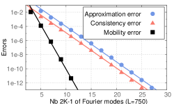
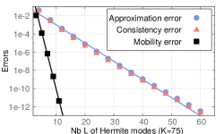
Refer to caption
Refer to caption
Figure 2: Approximation error, consistency error and error on the mobility as a function of the number of Fourier modes (Left) or Hermite modes (Right) for γ=1𝛾1\gamma=1. Logarithmic units are used on the ordinate axis. When the number of Hermite modes is large, the error on the mobility scales as 102.5Ksuperscript102.5𝐾10^{-2.5K}, while the approximation and consistency errors both scale as 10Ksuperscript10𝐾10^{-K}. When the number of Fourier modes is large, the error on the mobility scales as 101.25Lsuperscript101.25𝐿10^{-1.25L}, while the approximation and consistency errors both scale as 100.2Lsuperscript100.2𝐿10^{-0.2L}.

As an illustration of our approach, we plot the value of the self-diffusion as a function of γ𝛾\gamma in Figure 3, as already done in [25] using Monte-Carlo techniques and in [24] using a very similar spectral method. We indeed retrieve the scaling Dγ1similar-to𝐷superscript𝛾1D\sim\gamma^{-1} proved in [25]. This computation can be done in a matter of seconds as it involves a single inversion of a sparse matrix of size KL=5000𝐾𝐿5000KL=5000 for each value of the friction γ𝛾\gamma. It is thus much faster that a standard Monte-Carlo simulation. This approach however becomes intractable when the dimension increases.
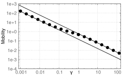
Refer to caption
Figure 3: Self-diffusion as a function of the friction γ𝛾\gamma. It scales as γ1superscript𝛾1\gamma^{-1} both for small γ𝛾\gamma (with prefactor 0.150.150.15) and large γ𝛾\gamma (with prefactor 0.60.60.6).

Estimates on the spectral gap.

In order to illustrate the statements of Proposition 4, we compute the relative error between the spectral gap of \mathcal{L} (approximated using a very large discretization basis) and the spectral gap of the matrix 𝐋^^𝐋\widehat{\mathbf{L}}; see Figure 5. The spectral gap is close to the value min(γ,γ1)𝛾superscript𝛾1\min(\gamma,\gamma^{-1}) obtained when V=0𝑉0V=0 (see [19]), with deviations essentially around γ=1𝛾1\gamma=1. Note on Figure 4 that the relative error on the spectral gap decays exponentially with K𝐾K and L𝐿L. Let us also emphasize that, as suggested by (23), the relative error on the spectral gap is bounded uniformly with respect to γ𝛾\gamma for any K,L𝐾𝐿K,L. We also observe that in the overdamped limit γ𝛾\gamma\to\infty the relative error depends only on the discretization accuracy in the position variable. This is due to the fact that the resolvent 1superscript1\mathcal{L}^{-1} converges in this regime to an operator acting only on the position variables [22].
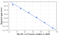
Refer to caption
Refer to caption
Refer to caption
Figure 4: Error on the spectral gap as a function of the size of the basis in three cases for γ=1𝛾1\gamma=1. For a large number of Hermite modes the error scales approximatively as 101.2(2K1)superscript101.22𝐾110^{-1.2(2K-1)} (top left); for a large number of Fourier modes it scales approximatively as 100.32Lsuperscript100.32𝐿10^{-0.32L} (top right); and for L=2(2K1)𝐿22𝐾1L=2(2K-1) it scales approximatively as 103.8Lsuperscript103.8𝐿10^{-3.8L} (bottom).
Refer to caption
Refer to caption
Figure 5: Left: Spectral gap as a function of the friction γ𝛾\gamma. Right: Relative error on the spectral gap as a function of γ𝛾\gamma for several couples K,L𝐾𝐿K,L. Note that the curve corresponding to K=3,L=8formulae-sequence𝐾3𝐿8K=3,L=8 coincides with K=5,L=8formulae-sequence𝐾5𝐿8K=5,L=8 for γ𝛾\gamma small and with K=3,L=20formulae-sequence𝐾3𝐿20K=3,L=20 for γ𝛾\gamma large.

Acknowledgements

We thank Alexandre Ern, Tony Lelièvre and François Madiot (CERMICS), as well as Greg Pavliotis and Urbain Vaes (Imperial College) for helpful discussions. This work is supported by the Agence Nationale de la Recherche under grant ANR-14-CE23-0012 (COSMOS); as well as the European Research Council under the European Union’s Seventh Framework Programme (FP/2007-2013) – ERC Grant Agreement number 614492. We also benefited from the scientific environment of the Laboratoire International Associé between the Centre National de la Recherche Scientifique and the University of Illinois at Urbana-Champaign. Finally, we acknowledge the support from the International Centre for Theoretical Sciences (ICTS) for the program Non-equilibrium statistical physics (ICTS/Prog-NESP/2015/10).

Appendix A Proof of Theorem 1 (L2(μ)superscriptL2𝜇{\mathrm{L}^{2}(\mu)} hypocoercivity)

We recall in this section the proof of Theorem 1, as presented in [7, 8]. We start with the proofs of the technical results presented at the end of Section 2.

Proof of Lemma 1.

Consider φΠ0𝒞𝜑subscriptΠ0𝒞\varphi\in\Pi_{0}\mathscr{C}. A simple computation shows that

hamΠp=1βqpΠp=(pm)qΠp,subscripthamsubscriptΠ𝑝1𝛽subscript𝑞superscriptsubscript𝑝subscriptΠ𝑝superscript𝑝𝑚topsubscript𝑞subscriptΠ𝑝\mathcal{L}_{\rm{ham}}\Pi_{p}=\frac{1}{\beta}\nabla_{q}\nabla_{p}^{*}\Pi_{p}=\left(\frac{p}{m}\right)^{\top}\nabla_{q}\Pi_{p}, (63)

which immediately implies that hamΠpφsubscripthamsubscriptΠ𝑝𝜑\mathcal{L}_{\rm{ham}}\Pi_{p}\varphi has average 0 with respect to κ(dp)𝜅𝑝\kappa(\differential p) for any q𝒟𝑞𝒟q\in\mathcal{D}. Therefore, ΠphamΠp=0subscriptΠ𝑝subscripthamsubscriptΠ𝑝0\Pi_{p}\mathcal{L}_{\rm{ham}}\Pi_{p}=0, which implies A=A(1Πp)𝐴𝐴1subscriptΠ𝑝A=A(1-\Pi_{p}).

By definition of the operator A𝐴A, it also holds

Aφ+(hamΠp)(hamΠp)Aφ=(hamΠp)φ.𝐴𝜑superscriptsubscripthamsubscriptΠ𝑝subscripthamsubscriptΠ𝑝𝐴𝜑superscriptsubscripthamsubscriptΠ𝑝𝜑A\varphi+(\mathcal{L}_{\rm{ham}}\Pi_{p})^{*}(\mathcal{L}_{\rm{ham}}\Pi_{p})A\varphi=(\mathcal{L}_{\rm{ham}}\Pi_{p})^{*}\varphi.

This identity immediately implies that ΠpA=AsubscriptΠ𝑝𝐴𝐴\Pi_{p}A=A. Taking the scalar product with Aφ𝐴𝜑A\varphi, we obtain, using hamA=hamΠpA=(1Πp)hamAsubscriptham𝐴subscripthamsubscriptΠ𝑝𝐴1subscriptΠ𝑝subscriptham𝐴\mathcal{L}_{\rm{ham}}A=\mathcal{L}_{\rm{ham}}\Pi_{p}A=(1-\Pi_{p})\mathcal{L}_{\rm{ham}}A:

Aφ2+hamAφ2superscriptnorm𝐴𝜑2superscriptnormsubscriptham𝐴𝜑2\displaystyle\|A\varphi\|^{2}+\|\mathcal{L}_{\rm{ham}}A\varphi\|^{2} =hamAφ,φ=hamAφ,(1Πp)φabsentsubscriptham𝐴𝜑𝜑subscriptham𝐴𝜑1subscriptΠ𝑝𝜑\displaystyle=\left\langle\mathcal{L}_{\rm{ham}}A\varphi,\varphi\right\rangle=\left\langle\mathcal{L}_{\rm{ham}}A\varphi,(1-\Pi_{p})\varphi\right\rangle (64)
(1Πp)φhamAφabsentnorm1subscriptΠ𝑝𝜑normsubscriptham𝐴𝜑\displaystyle\leqslant\|(1-\Pi_{p})\varphi\|\,\|\mathcal{L}_{\rm{ham}}A\varphi\|
14(1Πp)φ2+hamAφ2.absent14superscriptnorm1subscriptΠ𝑝𝜑2superscriptnormsubscriptham𝐴𝜑2\displaystyle\leqslant\frac{1}{4}\|(1-\Pi_{p})\varphi\|^{2}+\|\mathcal{L}_{\rm{ham}}A\varphi\|^{2}.

The last inequality gives Aφ(1Π)φ/2norm𝐴𝜑norm1Π𝜑2\|A\varphi\|\leqslant\|(1-\Pi)\varphi\|/2, while the second one implies that hamAφ(1Πp)φnormsubscriptham𝐴𝜑norm1subscriptΠ𝑝𝜑\|\mathcal{L}_{\rm{ham}}A\varphi\|\leqslant\|(1-\Pi_{p})\varphi\|. The conclusion is finally obtained by density of 𝒞𝒞\mathscr{C} in L2(μ)superscriptL2𝜇{\mathrm{L}^{2}(\mu)}. ∎

The key element to prove Proposition 1 is the following coercivity estimates, respectively called “microscopic” and “macroscopic” coercivity in [7, 8].

Proposition 6 (Coercivity properties).

The operators FDsubscriptFD{\mathcal{L}_{\mathrm{FD}}} and hamΠpsubscripthamsubscriptΠ𝑝\mathcal{L}_{\rm{ham}}\Pi_{p} satisfy the following coercivity properties:

φ𝒞,FDφ,φ1m(1Πp)φ2,formulae-sequencefor-all𝜑𝒞subscriptFD𝜑𝜑1𝑚superscriptnorm1subscriptΠ𝑝𝜑2\forall\varphi\in\mathscr{C},\qquad-\left\langle{\mathcal{L}_{\mathrm{FD}}}\varphi,\varphi\right\rangle\geqslant\frac{1}{m}\|(1-\Pi_{p})\varphi\|^{2}, (65)
φ𝒞L02(μ),hamΠpφ2CνβmΠpφ2,formulae-sequencefor-all𝜑𝒞superscriptsubscriptL02𝜇superscriptnormsubscripthamsubscriptΠ𝑝𝜑2subscript𝐶𝜈𝛽𝑚superscriptnormsubscriptΠ𝑝𝜑2\forall\varphi\in\mathscr{C}\cap{\mathrm{L}_{0}^{2}(\mu)},\qquad\|\mathcal{L}_{\rm{ham}}\Pi_{p}\varphi\|^{2}\geqslant\frac{C_{\nu}}{\beta m}\|\Pi_{p}\varphi\|^{2}, (66)

where Cνsubscript𝐶𝜈C_{\nu} is defined in (8). As a corollary, the following inequality holds in the sense of symmetric operators on L02(μ)superscriptsubscriptL02𝜇{\mathrm{L}_{0}^{2}(\mu)}:

AhamΠpλhamΠp,λham=1(1+Cνβm)1>0.formulae-sequence𝐴subscripthamsubscriptΠ𝑝subscript𝜆hamsubscriptΠ𝑝subscript𝜆ham1superscript1subscript𝐶𝜈𝛽𝑚10A\mathcal{L}_{\rm{ham}}\Pi_{p}\geqslant\lambda_{\rm{ham}}\Pi_{p},\qquad\lambda_{\rm{ham}}=1-\left(1+\frac{C_{\nu}}{\beta m}\right)^{-1}>0. (67)
Proof.

The inequality (65) directly results from a Poincaré inequality for the Gaussian measure κ𝜅\kappa (see [5]), the position q𝑞q being seen as a parameter. Indeed, for a given φ𝒞𝜑𝒞\varphi\in\mathscr{C},

q𝒟,D|pφ(q,p)|2κ(dp)βmD|(1Πp)φ(q,p)|2κ(dp)formulae-sequencefor-all𝑞𝒟subscriptsuperscript𝐷superscriptsubscript𝑝𝜑𝑞𝑝2𝜅𝑝𝛽𝑚subscriptsuperscript𝐷superscript1subscriptΠ𝑝𝜑𝑞𝑝2𝜅𝑝\forall q\in\mathcal{D},\qquad\int_{\mathbb{R}^{D}}\left|\nabla_{p}\varphi(q,p)\right|^{2}\,\kappa(\differential p)\geqslant\frac{\beta}{m}\int_{\mathbb{R}^{D}}\left|(1-\Pi_{p})\varphi(q,p)\right|^{2}\,\kappa(\differential p) (68)

Integrating against ν𝜈\nu and noting that FDφ,φ=β1pφ2subscriptFD𝜑𝜑superscript𝛽1superscriptnormsubscript𝑝𝜑2-\left\langle{\mathcal{L}_{\mathrm{FD}}}\varphi,\varphi\right\rangle=\beta^{-1}\|\nabla_{p}\varphi\|^{2} leads to the desired inequality.

To prove (66), we use (63), which leads to

hamΠpφL2(μ)2=1βmqΠpφL2(ν)2.superscriptsubscriptnormsubscripthamsubscriptΠ𝑝𝜑superscriptL2𝜇21𝛽𝑚superscriptsubscriptnormsubscript𝑞subscriptΠ𝑝𝜑superscriptL2𝜈2\|\mathcal{L}_{\rm{ham}}\Pi_{p}\varphi\|_{\mathrm{L}^{2}(\mu)}^{2}=\frac{1}{\beta m}\|\nabla_{q}\Pi_{p}\varphi\|_{\mathrm{L}^{2}(\nu)}^{2}. (69)

The conclusion then follows from the Poincaré inequality (8), since, for φ𝒞L02(μ)𝜑𝒞superscriptsubscriptL02𝜇\varphi\in\mathscr{C}\cap{\mathrm{L}_{0}^{2}(\mu)}, the function ΠpφsubscriptΠ𝑝𝜑\Pi_{p}\varphi has average 0 with respect to ν𝜈\nu (namely, 𝔼ν[Πpφ]=𝔼μ[φ]=0subscript𝔼𝜈delimited-[]subscriptΠ𝑝𝜑subscript𝔼𝜇delimited-[]𝜑0\mathbb{E}_{\nu}[\Pi_{p}\varphi]=\mathbb{E}_{\mu}[\varphi]=0).

The macroscopic coercivity (66) allows to write (hamΠp)(hamΠp)CνβmΠpsuperscriptsubscripthamsubscriptΠ𝑝subscripthamsubscriptΠ𝑝subscript𝐶𝜈𝛽𝑚subscriptΠ𝑝(\mathcal{L}_{\rm{ham}}\Pi_{p})^{*}(\mathcal{L}_{\rm{ham}}\Pi_{p})\geqslant\frac{C_{\nu}}{\beta m}\Pi_{p} in the sense of symmetric operators on L02(μ)superscriptsubscriptL02𝜇{\mathrm{L}_{0}^{2}(\mu)}. Moreover,

AhamΠp=[1+(hamΠp)(hamΠp)]1(hamΠp)(hamΠp).𝐴subscripthamsubscriptΠ𝑝superscriptdelimited-[]1superscriptsubscripthamsubscriptΠ𝑝subscripthamsubscriptΠ𝑝1superscriptsubscripthamsubscriptΠ𝑝subscripthamsubscriptΠ𝑝A\mathcal{L}_{\rm{ham}}\Pi_{p}=\left[1+(\mathcal{L}_{\rm{ham}}\Pi_{p})^{*}(\mathcal{L}_{\rm{ham}}\Pi_{p})\right]^{-1}(\mathcal{L}_{\rm{ham}}\Pi_{p})^{*}(\mathcal{L}_{\rm{ham}}\Pi_{p}).

Since (hamΠp)(hamΠp)superscriptsubscripthamsubscriptΠ𝑝subscripthamsubscriptΠ𝑝(\mathcal{L}_{\rm{ham}}\Pi_{p})^{*}(\mathcal{L}_{\rm{ham}}\Pi_{p}) is self-adjoint and the function xx/(1+x)=11/(1+x)maps-to𝑥𝑥1𝑥111𝑥x\mapsto x/(1+x)=1-1/(1+x) is increasing, the inequality (67) follows by spectral calculus. ∎

Another technical argument is the boundedness of certain operators, which appear in the proof of Proposition 1.

Lemma 4.

For any superscript\ell\in\mathbb{N}^{*}, i{1,2,,D}𝑖12𝐷i\in\{1,2,\dots,D\} and φL2(μ)𝜑superscriptL2𝜇\varphi\in{\mathrm{L}^{2}(\mu)},

ΠppiφL2(ν)(βm)!(1Πp)φ.subscriptnormsubscriptΠ𝑝superscriptsubscriptsubscript𝑝𝑖𝜑superscriptL2𝜈superscript𝛽𝑚norm1subscriptΠ𝑝𝜑\|\Pi_{p}\partial_{p_{i}}^{\ell}\varphi\|_{\mathrm{L}^{2}(\nu)}\leqslant\sqrt{\left(\frac{\beta}{m}\right)^{\ell}\ell!}\,\|(1-\Pi_{p})\varphi\|.

In particular, Πppi=(pi)Πpβ!normsubscriptΠ𝑝superscriptsubscriptsubscript𝑝𝑖normsuperscriptsuperscriptsubscriptsubscript𝑝𝑖subscriptΠ𝑝superscript𝛽\left\|\Pi_{p}\partial_{p_{i}}^{\ell}\right\|=\left\|\left(\partial_{p_{i}}^{*}\right)^{\ell}\Pi_{p}\right\|\leqslant\sqrt{\beta^{\ell}\ell!}.

Proof.

Fix φ𝒞𝜑𝒞\varphi\in\mathscr{C}. For q𝒟𝑞𝒟q\in\mathcal{D},

(Πppinφ)(q)=D(pin(1Πp)φ)(q,p)κ(dp)=D(1Πp)φ(q,p)(pi)n𝟏κ(dp).subscriptΠ𝑝superscriptsubscriptsubscript𝑝𝑖𝑛𝜑𝑞subscriptsuperscript𝐷superscriptsubscriptsubscript𝑝𝑖𝑛1subscriptΠ𝑝𝜑𝑞𝑝𝜅𝑝subscriptsuperscript𝐷1subscriptΠ𝑝𝜑𝑞𝑝superscriptsuperscriptsubscriptsubscript𝑝𝑖𝑛1𝜅𝑝\left(\Pi_{p}\partial_{p_{i}}^{n}\varphi\right)(q)=\int_{\mathbb{R}^{D}}\left(\partial_{p_{i}}^{n}(1-\Pi_{p})\varphi\right)(q,p)\,\kappa(\differential p)=\int_{\mathbb{R}^{D}}(1-\Pi_{p})\varphi(q,p)\,(\partial_{p_{i}}^{*})^{n}\mathbf{1}\,\kappa(\differential p).

Denoting by H(pi)=(m/β)/2!1/2(pi)𝟏subscript𝐻subscript𝑝𝑖superscript𝑚𝛽2superscript12superscriptsuperscriptsubscriptsubscript𝑝𝑖1H_{\ell}(p_{i})=(m/\beta)^{\ell/2}\ell!^{-1/2}(\partial_{p_{i}}^{*})^{\ell}\mathbf{1} the Hermite polynomials in the variable pisubscript𝑝𝑖p_{i} (which, we recall, are such that HL2(κ)=1subscriptnormsubscript𝐻superscriptL2𝜅1\|H_{\ell}\|_{{\mathrm{L}^{2}(\kappa)}}=1), a Cauchy–Schwarz inequality shows that

ΠppiφL2(ν)2superscriptsubscriptnormsubscriptΠ𝑝superscriptsubscriptsubscript𝑝𝑖𝜑superscriptL2𝜈2\displaystyle\|\Pi_{p}\partial_{p_{i}}^{\ell}\varphi\|_{\mathrm{L}^{2}(\nu)}^{2} 𝒟(D|(1Πp)φ(q,p)||(βm)!H(pi)|κ(dp))2ν(dq)absentsubscript𝒟superscriptsubscriptsuperscript𝐷1subscriptΠ𝑝𝜑𝑞𝑝superscript𝛽𝑚subscript𝐻subscript𝑝𝑖𝜅𝑝2𝜈𝑞\displaystyle\leqslant\int_{\mathcal{D}}\left(\int_{\mathbb{R}^{D}}|(1-\Pi_{p})\varphi(q,p)|\,\left|\sqrt{\left(\frac{\beta}{m}\right)^{\ell}\ell!}H_{\ell}(p_{i})\right|\kappa(\differential p)\right)^{2}\nu(\differential q)
(βm)!𝒟(1Πp)φ(q,)L2(κ)2HL2(κ)2ν(dq)=(βm)!(1Πp)φ2,absentsuperscript𝛽𝑚subscript𝒟superscriptsubscriptnorm1subscriptΠ𝑝𝜑𝑞superscriptL2𝜅2superscriptsubscriptnormsubscript𝐻superscriptL2𝜅2𝜈𝑞superscript𝛽𝑚superscriptnorm1subscriptΠ𝑝𝜑2\displaystyle\leqslant\left(\frac{\beta}{m}\right)^{\ell}\ell!\int_{\mathcal{D}}\|(1-\Pi_{p})\varphi(q,\cdot)\|_{\mathrm{L}^{2}(\kappa)}^{2}\|H_{\ell}\|_{\mathrm{L}^{2}(\kappa)}^{2}\nu(\differential q)=\left(\frac{\beta}{m}\right)^{\ell}\ell!\|(1-\Pi_{p})\varphi\|^{2},

which gives the claimed result. ∎

Proposition 7 (Boundedness of auxiliary operators).

There exist Rham>0subscript𝑅ham0R_{\rm ham}>0 such that

φ𝒞,{Aham(1Πp)φRham(1Πp)φ,AFDφ12m(1Πp)φ.\forall\varphi\in\mathscr{C},\qquad\left\{\begin{aligned} \|A\mathcal{L}_{\rm{ham}}(1-\Pi_{p})\varphi\|&\leqslant R_{\rm ham}\|(1-\Pi_{p})\varphi\|,\\ \|A{\mathcal{L}_{\mathrm{FD}}}\varphi\|&\leqslant\frac{1}{2m}\|(1-\Pi_{p})\varphi\|.\end{aligned}\right. (70)
Proof.

The first task is to give a more explicit expression of the operator A𝐴A. In the following we use frequently the fact that operators acting only on the variables q𝑞q (such as qsubscript𝑞\nabla_{q} and qsuperscriptsubscript𝑞\nabla_{q}^{*}) commute with operators acting only on variables p𝑝p (such as psubscript𝑝\nabla_{p}, psuperscriptsubscript𝑝\nabla_{p}^{*} and ΠpsubscriptΠ𝑝\Pi_{p}). Moreover the relations piΠp=0subscriptsubscript𝑝𝑖subscriptΠ𝑝0\partial_{p_{i}}\Pi_{p}=0, Πppi=0subscriptΠ𝑝superscriptsubscriptsubscript𝑝𝑖0\Pi_{p}\partial_{p_{i}}^{*}=0 and Πppipj=pipjΠp=βmΠpδijsubscriptΠ𝑝subscriptsubscript𝑝𝑖superscriptsubscriptsubscript𝑝𝑗subscriptsubscript𝑝𝑖superscriptsubscriptsubscript𝑝𝑗subscriptΠ𝑝𝛽𝑚subscriptΠ𝑝subscript𝛿𝑖𝑗\Pi_{p}\partial_{p_{i}}\partial_{p_{j}}^{*}=\partial_{p_{i}}\partial_{p_{j}}^{*}\Pi_{p}=\frac{\beta}{m}\Pi_{p}\delta_{ij} allow to simplify the action of (hamΠp)(hamΠp)superscriptsubscripthamsubscriptΠ𝑝subscripthamsubscriptΠ𝑝(\mathcal{L}_{\rm{ham}}\Pi_{p})^{*}(\mathcal{L}_{\rm{ham}}\Pi_{p}) as follows:

(hamΠp)(hamΠp)superscriptsubscripthamsubscriptΠ𝑝subscripthamsubscriptΠ𝑝\displaystyle(\mathcal{L}_{\rm{ham}}\Pi_{p})^{*}(\mathcal{L}_{\rm{ham}}\Pi_{p}) =1β2Πp(pqqp)(pqqp)Πpabsent1superscript𝛽2subscriptΠ𝑝superscriptsubscript𝑝subscript𝑞superscriptsubscript𝑞subscript𝑝superscriptsubscript𝑝subscript𝑞superscriptsubscript𝑞subscript𝑝subscriptΠ𝑝\displaystyle=-\frac{1}{\beta^{2}}\Pi_{p}(\nabla_{p}^{*}\nabla_{q}-\nabla_{q}^{*}\nabla_{p})(\nabla_{p}^{*}\nabla_{q}-\nabla_{q}^{*}\nabla_{p})\Pi_{p}
=1β2Πp(qp)(pq)Πp=1βmqqΠp.absent1superscript𝛽2subscriptΠ𝑝superscriptsubscript𝑞subscript𝑝superscriptsubscript𝑝subscript𝑞subscriptΠ𝑝1𝛽𝑚superscriptsubscript𝑞subscript𝑞subscriptΠ𝑝\displaystyle=\frac{1}{\beta^{2}}\Pi_{p}(\nabla_{q}^{*}\nabla_{p})(\nabla_{p}^{*}\nabla_{q})\Pi_{p}=\frac{1}{\beta m}\nabla_{q}^{*}\nabla_{q}\Pi_{p}.

The operator A𝐴A can therefore be reformulated as

A=1β(1+1βmqq)1qΠpp.𝐴1𝛽superscript11𝛽𝑚superscriptsubscript𝑞subscript𝑞1superscriptsubscript𝑞subscriptΠ𝑝subscript𝑝A=\frac{1}{\beta}\left(1+\frac{1}{\beta m}\nabla_{q}^{*}\nabla_{q}\right)^{-1}\nabla_{q}^{*}\Pi_{p}\nabla_{p}. (71)

To obtain bounds on the operator Aham(1Πp)𝐴subscriptham1subscriptΠ𝑝A\mathcal{L}_{\rm{ham}}(1-\Pi_{p}), we next consider its adjoint:

(1Πp)hamA1subscriptΠ𝑝subscripthamsuperscript𝐴\displaystyle-(1-\Pi_{p})\mathcal{L}_{\rm{ham}}A^{*} =1β2(1Πp)(pqqp)pqΠp(1+1βmqq)1absent1superscript𝛽21subscriptΠ𝑝superscriptsubscript𝑝subscript𝑞superscriptsubscript𝑞subscript𝑝superscriptsubscript𝑝subscript𝑞subscriptΠ𝑝superscript11𝛽𝑚superscriptsubscript𝑞subscript𝑞1\displaystyle=-\frac{1}{\beta^{2}}(1-\Pi_{p})\left(\nabla_{p}^{*}\nabla_{q}-\nabla_{q}^{*}\nabla_{p}\right)\nabla_{p}^{*}\nabla_{q}\Pi_{p}\left(1+\frac{1}{\beta m}\nabla_{q}^{*}\nabla_{q}\right)^{-1}
=1β2(1Πp)(pqpqβmqq)Πp(1+1βmqq)1absent1superscript𝛽21subscriptΠ𝑝superscriptsubscript𝑝subscript𝑞superscriptsubscript𝑝subscript𝑞𝛽𝑚superscriptsubscript𝑞subscript𝑞subscriptΠ𝑝superscript11𝛽𝑚superscriptsubscript𝑞subscript𝑞1\displaystyle=-\frac{1}{\beta^{2}}(1-\Pi_{p})\left(\nabla_{p}^{*}\nabla_{q}\nabla_{p}^{*}\nabla_{q}-\frac{\beta}{m}\nabla_{q}^{*}\nabla_{q}\right)\Pi_{p}\left(1+\frac{1}{\beta m}\nabla_{q}^{*}\nabla_{q}\right)^{-1}
=1β2(1Πp)pqpqΠp(1+1βmqq)1,absent1superscript𝛽21subscriptΠ𝑝superscriptsubscript𝑝subscript𝑞superscriptsubscript𝑝subscript𝑞subscriptΠ𝑝superscript11𝛽𝑚superscriptsubscript𝑞subscript𝑞1\displaystyle=-\frac{1}{\beta^{2}}(1-\Pi_{p})\nabla_{p}^{*}\nabla_{q}\nabla_{p}^{*}\nabla_{q}\Pi_{p}\left(1+\frac{1}{\beta m}\nabla_{q}^{*}\nabla_{q}\right)^{-1},

where we used (1Πp)qqΠp=01subscriptΠ𝑝superscriptsubscript𝑞subscript𝑞subscriptΠ𝑝0(1-\Pi_{p})\nabla_{q}^{*}\nabla_{q}\Pi_{p}=0 in the last line. Moreover, the operator

pqpqΠp=i,j=1DpipjΠpqiqjsuperscriptsubscript𝑝subscript𝑞superscriptsubscript𝑝subscript𝑞subscriptΠ𝑝superscriptsubscript𝑖𝑗1𝐷superscriptsubscriptsubscript𝑝𝑖superscriptsubscriptsubscript𝑝𝑗subscriptΠ𝑝subscriptsubscript𝑞𝑖subscriptsubscript𝑞𝑗\nabla_{p}^{*}\nabla_{q}\nabla_{p}^{*}\nabla_{q}\Pi_{p}=\sum_{i,j=1}^{D}\partial_{p_{i}}^{*}\partial_{p_{j}}^{*}\Pi_{p}\partial_{q_{i}}\partial_{q_{j}}

is bounded from H2(ν)superscriptH2𝜈\mathrm{H}^{2}(\nu) to L2(μ)superscriptL2𝜇{\mathrm{L}^{2}(\mu)} according to Lemma 4. Moreover, as proved in [8], Assumption 1 ensures that the operator Πp(1+1βmqq)1subscriptΠ𝑝superscript11𝛽𝑚superscriptsubscript𝑞subscript𝑞1\Pi_{p}\left(1+\frac{1}{\beta m}\nabla_{q}^{*}\nabla_{q}\right)^{-1} is bounded from L2(μ)superscriptL2𝜇{\mathrm{L}^{2}(\mu)} to H2(ν)superscriptH2𝜈\mathrm{H}^{2}(\nu). In conclusion, (1Πp)hamA1subscriptΠ𝑝subscripthamsuperscript𝐴-(1-\Pi_{p})\mathcal{L}_{\rm{ham}}A^{*} is bounded on L2(μ)superscriptL2𝜇{\mathrm{L}^{2}(\mu)}.

The boundedness of the operator AFD𝐴subscriptFDA{\mathcal{L}_{\mathrm{FD}}} comes from the fact that

ΠphamFDsubscriptΠ𝑝subscripthamsubscriptFD\displaystyle\Pi_{p}\mathcal{L}_{\rm{ham}}{\mathcal{L}_{\mathrm{FD}}} =1β2Πp(pqqp)pp=1β2Πpqpppabsent1superscript𝛽2subscriptΠ𝑝superscriptsubscript𝑝subscript𝑞superscriptsubscript𝑞subscript𝑝superscriptsubscript𝑝subscript𝑝1superscript𝛽2subscriptΠ𝑝superscriptsubscript𝑞subscript𝑝superscriptsubscript𝑝subscript𝑝\displaystyle=-\frac{1}{\beta^{2}}\Pi_{p}\left(\nabla_{p}^{*}\nabla_{q}-\nabla_{q}^{*}\nabla_{p}\right)\nabla_{p}^{*}\nabla_{p}=\frac{1}{\beta^{2}}\Pi_{p}\nabla_{q}^{*}\nabla_{p}\nabla_{p}^{*}\nabla_{p}
=1βmΠpqp=1mΠpham.absent1𝛽𝑚subscriptΠ𝑝superscriptsubscript𝑞subscript𝑝1𝑚subscriptΠ𝑝subscriptham\displaystyle=\frac{1}{\beta m}\Pi_{p}\nabla_{q}^{*}\nabla_{p}=-\frac{1}{m}\Pi_{p}\mathcal{L}_{\rm{ham}}.

In conclusion, AFD=A/m𝐴subscriptFD𝐴𝑚A{\mathcal{L}_{\mathrm{FD}}}=-A/m, which gives the claimed result with Lemma 1. ∎

We can now proceed with the proof of Proposition 1.

Proof of Proposition 1.

Note first that, for a given φ𝒞𝜑𝒞\varphi\in\mathscr{C}, the entropy dissipation 𝒟[φ]𝒟delimited-[]𝜑\mathscr{D}[\varphi] can be explicitly written as

𝒟[φ]𝒟delimited-[]𝜑\displaystyle\mathscr{D}[\varphi] =γFDφ,φ+εAhamΠpφ,φ+εAham(1Πp)φ,φabsent𝛾subscriptFD𝜑𝜑𝜀𝐴subscripthamsubscriptΠ𝑝𝜑𝜑𝜀𝐴subscriptham1subscriptΠ𝑝𝜑𝜑\displaystyle=\left\langle-\gamma{\mathcal{L}_{\mathrm{FD}}}\varphi,\varphi\right\rangle+\varepsilon\left\langle A\mathcal{L}_{\rm{ham}}\Pi_{p}\varphi,\varphi\right\rangle+\varepsilon\left\langle A\mathcal{L}_{\rm{ham}}(1-\Pi_{p})\varphi,\varphi\right\rangle (72)
εhamAφ,φ+εγAFDφ,φ,𝜀subscriptham𝐴𝜑𝜑𝜀𝛾𝐴subscriptFD𝜑𝜑\displaystyle\ \ -\varepsilon\left\langle\mathcal{L}_{\rm{ham}}A\varphi,\varphi\right\rangle+\varepsilon\gamma\left\langle A{\mathcal{L}_{\mathrm{FD}}}\varphi,\varphi\right\rangle,

since FDA=FDΠpA=0subscriptFD𝐴subscriptFDsubscriptΠ𝑝𝐴0{\mathcal{L}_{\mathrm{FD}}}A={\mathcal{L}_{\mathrm{FD}}}\Pi_{p}A=0. Using respectively the properties (65), (67), (70) and Lemma 1, it follows

𝒟[φ]𝒟delimited-[]𝜑\displaystyle\mathscr{D}[\varphi] γm(1Πp)φ2+ελhamΠpφ2ε(Rham+γ2m)(1Πp)φΠpφabsent𝛾𝑚superscriptnorm1subscriptΠ𝑝𝜑2𝜀subscript𝜆hamsuperscriptnormsubscriptΠ𝑝𝜑2𝜀subscript𝑅ham𝛾2𝑚norm1subscriptΠ𝑝𝜑normsubscriptΠ𝑝𝜑\displaystyle\geqslant\frac{\gamma}{m}\|(1-\Pi_{p})\varphi\|^{2}+\varepsilon\lambda_{\rm{ham}}\|\Pi_{p}\varphi\|^{2}-\varepsilon\left(R_{\rm ham}+\frac{\gamma}{2m}\right)\|(1-\Pi_{p})\varphi\|\,\|\Pi_{p}\varphi\| (73)
εhamAφ,φ.𝜀subscriptham𝐴𝜑𝜑\displaystyle\ \ -\varepsilon\left\langle\mathcal{L}_{\rm{ham}}A\varphi,\varphi\right\rangle.

Since, by Lemma 1,

hamAφ,φ=(1Πp)hamΠpA(1Πp)φ,φ(1Πp)φ2,subscriptham𝐴𝜑𝜑1subscriptΠ𝑝subscripthamsubscriptΠ𝑝𝐴1subscriptΠ𝑝𝜑𝜑superscriptnorm1subscriptΠ𝑝𝜑2\left\langle\mathcal{L}_{\rm{ham}}A\varphi,\varphi\right\rangle=\left\langle(1-\Pi_{p})\mathcal{L}_{\rm{ham}}\Pi_{p}A(1-\Pi_{p})\varphi,\varphi\right\rangle\leqslant\|(1-\Pi_{p})\varphi\|^{2},

it holds 𝒟[φ]X𝐒X𝒟delimited-[]𝜑superscript𝑋top𝐒𝑋\mathscr{D}[\varphi]\geqslant X^{\top}\mathbf{S}X, where

X=(Πpφ(1Πp)φ),𝐒=(SS+/2S+/2S++),formulae-sequence𝑋matrixnormsubscriptΠ𝑝𝜑norm1subscriptΠ𝑝𝜑𝐒matrixsubscript𝑆absentsubscript𝑆absent2subscript𝑆absent2subscript𝑆absentX=\begin{pmatrix}\|\Pi_{p}\varphi\|\\ \|(1-\Pi_{p})\varphi\|\end{pmatrix},\qquad\mathbf{S}=\begin{pmatrix}S_{--}&S_{-+}/2\\ S_{-+}/2&S_{++}\end{pmatrix},

with

S=ελham,S+=ε(Rham+γ2m),S++=γmε.formulae-sequencesubscript𝑆absent𝜀subscript𝜆hamformulae-sequencesubscript𝑆absent𝜀subscript𝑅ham𝛾2𝑚subscript𝑆absent𝛾𝑚𝜀S_{--}=\varepsilon\lambda_{\rm{ham}},\qquad S_{-+}=-\varepsilon\left(R_{\rm ham}+\frac{\gamma}{2m}\right),\qquad S_{++}=\frac{\gamma}{m}-\varepsilon.

The smallest eigenvalue of 𝐒𝐒\mathbf{S} is

Λ(γ,ε)=S+S++212(SS++)2+(S+)2.Λ𝛾𝜀subscript𝑆absentsubscript𝑆absent212superscriptsubscript𝑆absentsubscript𝑆absent2superscriptsubscript𝑆absent2\Lambda(\gamma,\varepsilon)=\frac{S_{--}+S_{++}}{2}-\frac{1}{2}\sqrt{(S_{--}-S_{++})^{2}+(S_{-+})^{2}}.

In the limit γ0𝛾0\gamma\to 0, the parameter ε𝜀\varepsilon should be chosen of order γ𝛾\gamma in order for Λ(γ,ε)Λ𝛾𝜀\Lambda(\gamma,\varepsilon) to be positive (in particular for S++subscript𝑆absentS_{++} to remain positive). When γ+𝛾\gamma\to+\infty, the parameter ε𝜀\varepsilon should be chosen of order 1/γ1𝛾1/\gamma in order for the determinant of 𝐒𝐒\mathbf{S} to remain positive. We therefore consider the choice

ε=ε¯min(γ,γ1).𝜀¯𝜀𝛾superscript𝛾1\varepsilon=\overline{\varepsilon}\min(\gamma,\gamma^{-1}). (74)

It is then easy to check that there exists ε¯>0¯𝜀0\overline{\varepsilon}>0 sufficiently small such that Λ(γ,ε¯min(γ,γ1))>0Λ𝛾¯𝜀𝛾superscript𝛾10\Lambda(\gamma,\overline{\varepsilon}\min(\gamma,\gamma^{-1}))>0 for all γ>0𝛾0\gamma>0. Moreover, it can be proved that Λ(γ,ε¯min(γ,γ1))/γΛ𝛾¯𝜀𝛾superscript𝛾1𝛾\Lambda(\gamma,\overline{\varepsilon}\min(\gamma,\gamma^{-1}))/\gamma converges to a positive value as γ0𝛾0\gamma\to 0, while γΛ(γ,ε¯min(γ,γ1))𝛾Λ𝛾¯𝜀𝛾superscript𝛾1\gamma\Lambda(\gamma,\overline{\varepsilon}\min(\gamma,\gamma^{-1})) converges to a positive value as γ+𝛾\gamma\to+\infty. This gives the claimed result with λ~γ=Λ(γ,ε¯min(γ,γ1))subscript~𝜆𝛾Λ𝛾¯𝜀𝛾superscript𝛾1\widetilde{\lambda}_{\gamma}=\Lambda(\gamma,\overline{\varepsilon}\min(\gamma,\gamma^{-1})). ∎

The proof of Theorem 1 is now easy to obtain. Consider φ0Dom()L02(μ)subscript𝜑0DomsuperscriptsubscriptL02𝜇\varphi_{0}\in\mathrm{Dom}(\mathcal{L})\cap{\mathrm{L}_{0}^{2}(\mu)} (which contains H2(μ)L02(μ)superscriptH2𝜇superscriptsubscriptL02𝜇\mathrm{H}^{2}(\mu)\cap{\mathrm{L}_{0}^{2}(\mu)}) and introduce (t)=[φ(t)]𝑡delimited-[]𝜑𝑡\mathscr{H}(t)=\mathcal{H}[\varphi(t)], where φ(t)=etφ0Dom()𝜑𝑡superscripte𝑡subscript𝜑0Dom\varphi(t)=\mathrm{e}^{t\mathcal{L}}\varphi_{0}\in\mathrm{Dom}(\mathcal{L}) for any t0𝑡0t\geqslant 0. Then,

(t)=𝒟[φ(t)]λ~γφ(t)2.superscript𝑡𝒟delimited-[]𝜑𝑡subscript~𝜆𝛾superscriptnorm𝜑𝑡2\mathscr{H}^{\prime}(t)=-\mathscr{D}[\varphi(t)]\leqslant-\widetilde{\lambda}_{\gamma}\|\varphi(t)\|^{2}.

Using the norm equivalence (17) and the choice (74) for ε¯<1¯𝜀1\overline{\varepsilon}<1, it follows that

(t)2λ~γ1+ε¯min(γ,γ1)(t),superscript𝑡2subscript~𝜆𝛾1¯𝜀𝛾superscript𝛾1𝑡\mathscr{H}^{\prime}(t)\leqslant-\frac{2\widetilde{\lambda}_{\gamma}}{1+\overline{\varepsilon}\min(\gamma,\gamma^{-1})}\mathscr{H}(t),

so that, by a Gronwall estimate,

(t)(0)exp(2λ~γ1+ε¯min(γ,γ1)t).𝑡02subscript~𝜆𝛾1¯𝜀𝛾superscript𝛾1𝑡\mathscr{H}(t)\leqslant\mathscr{H}(0)\exp\left(-\frac{2\widetilde{\lambda}_{\gamma}}{1+\overline{\varepsilon}\min(\gamma,\gamma^{-1})}t\right).

Using again the norm equivalence (17), it follows that

φ(t)21+ε¯1ε¯e2λγtφ(0)2,superscriptnorm𝜑𝑡21¯𝜀1¯𝜀superscripte2subscript𝜆𝛾𝑡superscriptnorm𝜑02\|\varphi(t)\|^{2}\leqslant\frac{1+\overline{\varepsilon}}{1-\overline{\varepsilon}}\,\mathrm{e}^{-2\lambda_{\gamma}t}\|\varphi(0)\|^{2},

with the decay rate

λγ=λ~γ1+ε¯min(γ,γ1).subscript𝜆𝛾subscript~𝜆𝛾1¯𝜀𝛾superscript𝛾1\lambda_{\gamma}=\frac{\widetilde{\lambda}_{\gamma}}{1+\overline{\varepsilon}\min(\gamma,\gamma^{-1})}.

The desired estimate finally follows by density of Dom()Dom\mathrm{Dom}(\mathcal{L}) in L2(μ)superscriptL2𝜇{\mathrm{L}^{2}(\mu)}.

Appendix B Proof of technical estimates for the system considered in Section 4

We prove in this section that the conditions (29) and (21) allowing to apply the results of Section 3 hold for the system considered in Section 4. Recall that the condition M+𝑀M\to+\infty should be understood as K,L+𝐾𝐿K,L\to+\infty. Let us also emphasize that, although we perform the computations for the simple potential V(q)=1cos(q)𝑉𝑞1𝑞V(q)=1-\cos(q), the extension to a general trigonometric polynomial V𝑉V is straightforward.

Condition (29) and bound on uKnormsubscript𝑢𝐾\|\mathcal{L}u_{K}\|.

Since uMsubscript𝑢𝑀u_{M} depends only on the positions, it is denoted uKsubscript𝑢𝐾u_{K} and

uK2=uK2=1ΠKq𝟏2pqΠKq𝟏2=βqΠKq𝟏2ΠKq𝟏2.superscriptnormsubscript𝑢𝐾2superscriptnormsuperscriptsubscript𝑢𝐾21superscriptnormsuperscriptsubscriptΠ𝐾𝑞12superscriptnorm𝑝subscript𝑞superscriptsubscriptΠ𝐾𝑞12𝛽superscriptnormsubscript𝑞superscriptsubscriptΠ𝐾𝑞12superscriptnormsuperscriptsubscriptΠ𝐾𝑞12\|\mathcal{L}u_{K}\|^{2}=\|\mathcal{L}^{*}u_{K}\|^{2}=\frac{1}{\|\Pi_{K}^{q}\mathbf{1}\|^{2}}\left\|p\partial_{q}\Pi_{K}^{q}\mathbf{1}\right\|^{2}=\beta\frac{\|\partial_{q}\Pi_{K}^{q}\mathbf{1}\|^{2}}{\|\Pi_{K}^{q}\mathbf{1}\|^{2}}.

In order to estimate qΠKq𝟏normsubscript𝑞superscriptsubscriptΠ𝐾𝑞1\|\partial_{q}\Pi_{K}^{q}\mathbf{1}\|, we decompose ΠKq𝟏superscriptsubscriptΠ𝐾𝑞1\Pi_{K}^{q}\mathbf{1} in the basis under consideration as follows:

ΠKq𝟏=j=02K2gjGj,gj=ΠKq𝟏,Gj=𝒟Gj𝑑ν.formulae-sequencesuperscriptsubscriptΠ𝐾𝑞1superscriptsubscript𝑗02𝐾2subscript𝑔𝑗subscript𝐺𝑗subscript𝑔𝑗superscriptsubscriptΠ𝐾𝑞1subscript𝐺𝑗subscript𝒟subscript𝐺𝑗differential-d𝜈\Pi_{K}^{q}\mathbf{1}=\sum_{j=0}^{2K-2}g_{j}G_{j},\qquad g_{j}=\left\langle\Pi_{K}^{q}\mathbf{1},G_{j}\right\rangle=\int_{\mathcal{D}}G_{j}\,d\nu.

Then, using qΠKq𝟏=q(1ΠKq)𝟏subscript𝑞superscriptsubscriptΠ𝐾𝑞1subscript𝑞1superscriptsubscriptΠ𝐾𝑞1\partial_{q}\Pi_{K}^{q}\mathbf{1}=-\partial_{q}(1-\Pi_{K}^{q})\mathbf{1} and (with (59))

k1,qG2k=β4G2k3+kG2k1+β4G2k+1,qG2k1=β4G2k2kG2kβ4G2k+2,formulae-sequencefor-all𝑘1formulae-sequencesuperscriptsubscript𝑞subscript𝐺2𝑘𝛽4subscript𝐺2𝑘3𝑘subscript𝐺2𝑘1𝛽4subscript𝐺2𝑘1superscriptsubscript𝑞subscript𝐺2𝑘1𝛽4subscript𝐺2𝑘2𝑘subscript𝐺2𝑘𝛽4subscript𝐺2𝑘2\forall k\geqslant 1,\qquad\partial_{q}^{*}G_{2k}=-\frac{\beta}{4}G_{2k-3}+kG_{2k-1}+\frac{\beta}{4}G_{2k+1},\qquad\partial_{q}^{*}G_{2k-1}=\frac{\beta}{4}G_{2k-2}-kG_{2k}-\frac{\beta}{4}G_{2k+2}, (75)

it follows that, for K1𝐾1K\geqslant 1,

qΠKq𝟏2superscriptnormsubscript𝑞superscriptsubscriptΠ𝐾𝑞12\displaystyle\|\partial_{q}\Pi_{K}^{q}\mathbf{1}\|^{2} =jqΠKq𝟏,Gj2absentsubscript𝑗superscriptsubscript𝑞superscriptsubscriptΠ𝐾𝑞1subscript𝐺𝑗2\displaystyle=\sum_{j\in\mathbb{N}}\left\langle\partial_{q}\Pi_{K}^{q}\mathbf{1},G_{j}\right\rangle^{2}
=j=02K2q(1ΠKq)𝟏,Gj2+j=2K1+qΠKq𝟏,Gj2absentsuperscriptsubscript𝑗02𝐾2superscriptsubscript𝑞1superscriptsubscriptΠ𝐾𝑞1subscript𝐺𝑗2superscriptsubscript𝑗2𝐾1superscriptsubscript𝑞superscriptsubscriptΠ𝐾𝑞1subscript𝐺𝑗2\displaystyle=\sum_{j=0}^{2K-2}\left\langle-\partial_{q}(1-\Pi_{K}^{q})\mathbf{1},G_{j}\right\rangle^{2}+\sum_{j=2K-1}^{+\infty}\left\langle\partial_{q}\Pi_{K}^{q}\mathbf{1},G_{j}\right\rangle^{2}
=j=02K2𝔼ν[(1ΠKq)qGj]2+j=2K1+𝔼ν[ΠKqqGj]2absentsuperscriptsubscript𝑗02𝐾2subscript𝔼𝜈superscriptdelimited-[]1superscriptsubscriptΠ𝐾𝑞superscriptsubscript𝑞subscript𝐺𝑗2superscriptsubscript𝑗2𝐾1subscript𝔼𝜈superscriptdelimited-[]superscriptsubscriptΠ𝐾𝑞superscriptsubscript𝑞subscript𝐺𝑗2\displaystyle=\sum_{j=0}^{2K-2}\mathbb{E}_{\nu}\left[(1-\Pi_{K}^{q})\partial_{q}^{*}G_{j}\right]^{2}+\sum_{j=2K-1}^{+\infty}\mathbb{E}_{\nu}\left[\Pi_{K}^{q}\partial_{q}^{*}G_{j}\right]^{2}
=𝔼ν[(1ΠKq)qG2K3]2+𝔼ν[(1ΠKq)qG2K2]2+𝔼ν[ΠKqqG2K1]2+𝔼ν[ΠKqqG2K]2absentsubscript𝔼𝜈superscriptdelimited-[]1superscriptsubscriptΠ𝐾𝑞superscriptsubscript𝑞subscript𝐺2𝐾32subscript𝔼𝜈superscriptdelimited-[]1superscriptsubscriptΠ𝐾𝑞superscriptsubscript𝑞subscript𝐺2𝐾22subscript𝔼𝜈superscriptdelimited-[]superscriptsubscriptΠ𝐾𝑞superscriptsubscript𝑞subscript𝐺2𝐾12subscript𝔼𝜈superscriptdelimited-[]superscriptsubscriptΠ𝐾𝑞superscriptsubscript𝑞subscript𝐺2𝐾2\displaystyle=\mathbb{E}_{\nu}[(1-\Pi_{K}^{q})\partial_{q}^{*}G_{2K-3}]^{2}+\mathbb{E}_{\nu}[(1-\Pi_{K}^{q})\partial_{q}^{*}G_{2K-2}]^{2}+\mathbb{E}_{\nu}[\Pi_{K}^{q}\partial_{q}^{*}G_{2K-1}]^{2}+\mathbb{E}_{\nu}[\Pi_{K}^{q}\partial_{q}^{*}G_{2K}]^{2}
=β216(g2K2+g2K12+g2K22+g2K32)β216(1ΠK1q)𝟏2.absentsuperscript𝛽216superscriptsubscript𝑔2𝐾2superscriptsubscript𝑔2𝐾12superscriptsubscript𝑔2𝐾22superscriptsubscript𝑔2𝐾32superscript𝛽216superscriptnorm1superscriptsubscriptΠ𝐾1𝑞12\displaystyle=\frac{\beta^{2}}{16}\left(g_{2K}^{2}+g_{2K-1}^{2}+g_{2K-2}^{2}+g_{2K-3}^{2}\right)\leqslant\frac{\beta^{2}}{16}\left\|(1-\Pi_{K-1}^{q})\mathbf{1}\right\|^{2}.

Since 𝟏Hs(ν)1superscriptH𝑠𝜈\mathbf{1}\in{\mathrm{H}^{s}(\nu)} for any s𝑠s\in\mathbb{N}, it follows that (1ΠK1q)𝟏norm1superscriptsubscriptΠ𝐾1𝑞1\|(1-\Pi_{K-1}^{q})\mathbf{1}\| vanishes faster than any polynomial in K𝐾K in view of Lemma 2. This implies that qΠKq𝟏normsubscript𝑞superscriptsubscriptΠ𝐾𝑞1\|\partial_{q}\Pi_{K}^{q}\mathbf{1}\|, and hence uKnormsubscript𝑢𝐾\|\mathcal{L}u_{K}\| and uKnormsuperscriptsubscript𝑢𝐾\|\mathcal{L}^{*}u_{K}\|, vanish faster than any polynomial in K𝐾K. More precisely,

uK2=uK2β316(1ΠK1q)𝟏2ΠKq𝟏2β316(1ΠK1q)𝟏21(1ΠKq)𝟏2.superscriptnormsuperscriptsubscript𝑢𝐾2superscriptnormsubscript𝑢𝐾2superscript𝛽316superscriptnorm1superscriptsubscriptΠ𝐾1𝑞12superscriptnormsuperscriptsubscriptΠ𝐾𝑞12superscript𝛽316superscriptnorm1superscriptsubscriptΠ𝐾1𝑞121superscriptnorm1superscriptsubscriptΠ𝐾𝑞12\|\mathcal{L}^{*}u_{K}\|^{2}=\|\mathcal{L}u_{K}\|^{2}\leqslant\frac{\beta^{3}}{16}\frac{\left\|(1-\Pi_{K-1}^{q})\mathbf{1}\right\|^{2}}{\|\Pi_{K}^{q}\mathbf{1}\|^{2}}\leqslant\frac{\beta^{3}}{16}\frac{\left\|(1-\Pi_{K-1}^{q})\mathbf{1}\right\|^{2}}{1-\|(1-\Pi_{K}^{q})\mathbf{1}\|^{2}}. (76)

Condition (21).

Let us now prove that (A+A)(1ΠKL)ΠKLK,L0𝐾𝐿absentnorm𝐴superscript𝐴1subscriptΠ𝐾𝐿subscriptΠ𝐾𝐿0\|(A+A^{*})(1-\Pi_{KL})\mathcal{L}\Pi_{KL}\|\xrightarrow[K,L\to\infty]{}0 for the model under consideration. Introducing KL+=(1ΠKL)ΠKLsuperscriptsubscript𝐾𝐿absent1subscriptΠ𝐾𝐿subscriptΠ𝐾𝐿\mathcal{L}_{KL}^{+-}=(1-\Pi_{KL})\mathcal{L}\Pi_{KL}, we prove in fact that AKL+𝐴superscriptsubscript𝐾𝐿absentA\mathcal{L}_{KL}^{+-} and AKL+superscript𝐴superscriptsubscript𝐾𝐿absentA^{*}\mathcal{L}_{KL}^{+-} are bounded operators whose norms converge to 0 as K,L+𝐾𝐿K,L\to+\infty. In all this proof, we consider K1𝐾1K\geqslant 1 and L2𝐿2L\geqslant 2.

The first task is to provide a more explicit expression of KL+superscriptsubscript𝐾𝐿absent\mathcal{L}_{KL}^{+-}. We introduce to this end the operator DK+=ΠKqqΠKqsubscriptsuperscript𝐷absent𝐾superscriptsubscriptΠ𝐾perpendicular-to𝑞absentsubscript𝑞superscriptsubscriptΠ𝐾𝑞{D^{+-}_{K}}=\Pi_{K}^{q\perp}\partial_{q}\Pi_{K}^{q}. In view of (59),

DK+φsubscriptsuperscript𝐷absent𝐾𝜑\displaystyle{D^{+-}_{K}}\varphi =j=2K1+j=02K2φ,GjqGj,GjGj=β4(φ,G2K2G2K1φ,G2K3G2K).absentsuperscriptsubscriptsuperscript𝑗2𝐾1superscriptsubscript𝑗02𝐾2𝜑subscript𝐺𝑗subscript𝑞subscript𝐺𝑗subscript𝐺superscript𝑗subscript𝐺superscript𝑗𝛽4𝜑subscript𝐺2𝐾2subscript𝐺2𝐾1𝜑subscript𝐺2𝐾3subscript𝐺2𝐾\displaystyle=\sum_{j^{\prime}=2K-1}^{+\infty}\sum_{j=0}^{2K-2}\left\langle\varphi,G_{j}\right\rangle\left\langle\partial_{q}G_{j},G_{j^{\prime}}\right\rangle G_{j^{\prime}}=\frac{\beta}{4}\Big{(}\left\langle\varphi,G_{2K-2}\right\rangle G_{2K-1}-\left\langle\varphi,G_{2K-3}\right\rangle G_{2K}\Big{)}.

This shows that the operator DK+subscriptsuperscript𝐷absent𝐾{D^{+-}_{K}} is bounded on L2(μ)superscriptL2𝜇{\mathrm{L}^{2}(\mu)}, and in fact

DK+φβ4ΠK+1qΠKqφ.normsubscriptsuperscript𝐷absent𝐾𝜑𝛽4normsuperscriptsubscriptΠ𝐾1perpendicular-to𝑞absentsuperscriptsubscriptΠ𝐾𝑞𝜑\|{D^{+-}_{K}}\varphi\|\leqslant\frac{\beta}{4}\|\Pi_{K+1}^{q\perp}\Pi_{K}^{q}\varphi\|. (77)

Comparing (75) and (59), we also see that DK+=ΠKqqΠKq=ΠKqqΠKqsubscriptsuperscript𝐷absent𝐾superscriptsubscriptΠ𝐾perpendicular-to𝑞absentsubscript𝑞superscriptsubscriptΠ𝐾𝑞superscriptsubscriptΠ𝐾perpendicular-to𝑞absentsuperscriptsubscript𝑞superscriptsubscriptΠ𝐾𝑞{D^{+-}_{K}}=\Pi_{K}^{q\perp}\partial_{q}\Pi_{K}^{q}=\Pi_{K}^{q\perp}\partial_{q}^{*}\Pi_{K}^{q}. We can now compute more explicitly the action of KL+superscriptsubscript𝐾𝐿absent\mathcal{L}_{KL}^{+-} by noting that

βKL+=(1ΠKL)qpΠKL(1ΠKL)qpΠKLγ(1ΠKL)ppΠKL,𝛽superscriptsubscript𝐾𝐿absent1subscriptΠ𝐾𝐿subscript𝑞superscriptsubscript𝑝subscriptΠ𝐾𝐿1subscriptΠ𝐾𝐿superscriptsubscript𝑞subscript𝑝subscriptΠ𝐾𝐿𝛾1subscriptΠ𝐾𝐿superscriptsubscript𝑝subscript𝑝subscriptΠ𝐾𝐿\beta\mathcal{L}_{KL}^{+-}=(1-\Pi_{KL})\partial_{q}\partial_{p}^{*}\Pi_{KL}-(1-\Pi_{KL})\partial_{q}^{*}\partial_{p}\Pi_{KL}-\gamma(1-\Pi_{KL})\partial_{p}^{*}\partial_{p}\Pi_{KL},

where (1ΠKL)ppΠKL=01subscriptΠ𝐾𝐿superscriptsubscript𝑝subscript𝑝subscriptΠ𝐾𝐿0(1-\Pi_{KL})\partial_{p}^{*}\partial_{p}\Pi_{KL}=0 by (53), while (using (52) to write ΠL1pp=pΠLpsuperscriptsubscriptΠ𝐿1𝑝subscript𝑝subscript𝑝superscriptsubscriptΠ𝐿𝑝\Pi_{L-1}^{p}\partial_{p}=\partial_{p}\Pi_{L}^{p} and ΠL+1pp=pΠLpsuperscriptsubscriptΠ𝐿1𝑝superscriptsubscript𝑝superscriptsubscript𝑝superscriptsubscriptΠ𝐿𝑝\Pi_{L+1}^{p}\partial_{p}^{*}=\partial_{p}^{*}\Pi_{L}^{p})

(1ΠKL)qpΠKL1subscriptΠ𝐾𝐿subscript𝑞superscriptsubscript𝑝subscriptΠ𝐾𝐿\displaystyle(1-\Pi_{KL})\partial_{q}\partial_{p}^{*}\Pi_{KL} =(1ΠKqΠLp)qΠL+1ppΠKqabsent1superscriptsubscriptΠ𝐾𝑞superscriptsubscriptΠ𝐿𝑝subscript𝑞superscriptsubscriptΠ𝐿1𝑝superscriptsubscript𝑝superscriptsubscriptΠ𝐾𝑞\displaystyle=(1-\Pi_{K}^{q}\Pi_{L}^{p})\partial_{q}\Pi_{L+1}^{p}\partial_{p}^{*}\Pi_{K}^{q}
=(1ΠKqΠLp)q(ΠLp+ΠLp)ΠL+1ppΠKqabsent1superscriptsubscriptΠ𝐾𝑞superscriptsubscriptΠ𝐿𝑝subscript𝑞superscriptsubscriptΠ𝐿𝑝superscriptsubscriptΠ𝐿perpendicular-to𝑝absentsuperscriptsubscriptΠ𝐿1𝑝superscriptsubscript𝑝superscriptsubscriptΠ𝐾𝑞\displaystyle=(1-\Pi_{K}^{q}\Pi_{L}^{p})\partial_{q}(\Pi_{L}^{p}+\Pi_{L}^{p\perp})\Pi_{L+1}^{p}\partial_{p}^{*}\Pi_{K}^{q}
=(ΠLp+ΠLpΠL+1pΠKqΠLp)qpΠKqabsentsuperscriptsubscriptΠ𝐿𝑝superscriptsubscriptΠ𝐿perpendicular-to𝑝absentsuperscriptsubscriptΠ𝐿1𝑝superscriptsubscriptΠ𝐾𝑞superscriptsubscriptΠ𝐿𝑝subscript𝑞superscriptsubscript𝑝superscriptsubscriptΠ𝐾𝑞\displaystyle=(\Pi_{L}^{p}+\Pi_{L}^{p\perp}\Pi_{L+1}^{p}-\Pi_{K}^{q}\Pi_{L}^{p})\partial_{q}\partial_{p}^{*}\Pi_{K}^{q}
=ΠLp(1ΠKq)qpΠKq+qΠL+1pΠLppΠKqabsentsuperscriptsubscriptΠ𝐿𝑝1superscriptsubscriptΠ𝐾𝑞subscript𝑞superscriptsubscript𝑝superscriptsubscriptΠ𝐾𝑞subscript𝑞superscriptsubscriptΠ𝐿1𝑝superscriptsubscriptΠ𝐿perpendicular-to𝑝absentsuperscriptsubscript𝑝superscriptsubscriptΠ𝐾𝑞\displaystyle=\Pi_{L}^{p}(1-\Pi_{K}^{q})\partial_{q}\partial_{p}^{*}\Pi_{K}^{q}+\partial_{q}\Pi_{L+1}^{p}\Pi_{L}^{p\perp}\partial_{p}^{*}\Pi_{K}^{q}
=ΠLppDK++qpΠLpΠL1pΠKqabsentsuperscriptsubscriptΠ𝐿𝑝superscriptsubscript𝑝subscriptsuperscript𝐷absent𝐾subscript𝑞superscriptsubscript𝑝superscriptsubscriptΠ𝐿𝑝superscriptsubscriptΠ𝐿1perpendicular-to𝑝absentsuperscriptsubscriptΠ𝐾𝑞\displaystyle=\Pi_{L}^{p}\partial_{p}^{*}{D^{+-}_{K}}+\partial_{q}\partial_{p}^{*}\Pi_{L}^{p}\Pi_{L-1}^{p\perp}\Pi_{K}^{q}
=pΠL1pDK++qpΠL1pΠKL,absentsuperscriptsubscript𝑝superscriptsubscriptΠ𝐿1𝑝subscriptsuperscript𝐷absent𝐾subscript𝑞superscriptsubscript𝑝superscriptsubscriptΠ𝐿1perpendicular-to𝑝absentsubscriptΠ𝐾𝐿\displaystyle=\partial_{p}^{*}\Pi_{L-1}^{p}{D^{+-}_{K}}+\partial_{q}\partial_{p}^{*}\Pi_{L-1}^{p\perp}\Pi_{KL},

and

(1ΠKL)qpΠKL1subscriptΠ𝐾𝐿superscriptsubscript𝑞subscript𝑝subscriptΠ𝐾𝐿\displaystyle(1-\Pi_{KL})\partial_{q}^{*}\partial_{p}\Pi_{KL} =p(1ΠKqΠL+1p)qΠLpΠKq=pΠLp(1ΠKq)qΠKqabsentsubscript𝑝1superscriptsubscriptΠ𝐾𝑞superscriptsubscriptΠ𝐿1𝑝superscriptsubscript𝑞superscriptsubscriptΠ𝐿𝑝superscriptsubscriptΠ𝐾𝑞subscript𝑝superscriptsubscriptΠ𝐿𝑝1superscriptsubscriptΠ𝐾𝑞superscriptsubscript𝑞superscriptsubscriptΠ𝐾𝑞\displaystyle=\partial_{p}(1-\Pi_{K}^{q}\Pi_{L+1}^{p})\partial_{q}^{*}\Pi_{L}^{p}\Pi_{K}^{q}=\partial_{p}\Pi_{L}^{p}(1-\Pi_{K}^{q})\partial_{q}^{*}\Pi_{K}^{q}
=DK+pΠLp.absentsubscriptsuperscript𝐷absent𝐾subscript𝑝superscriptsubscriptΠ𝐿𝑝\displaystyle={D^{+-}_{K}}\partial_{p}\Pi_{L}^{p}.

Therefore,

βKL+=pΠL1pDK++qpΠL1pΠKLDK+pΠLp.𝛽superscriptsubscript𝐾𝐿absentsuperscriptsubscript𝑝superscriptsubscriptΠ𝐿1𝑝subscriptsuperscript𝐷absent𝐾subscript𝑞superscriptsubscript𝑝superscriptsubscriptΠ𝐿1perpendicular-to𝑝absentsubscriptΠ𝐾𝐿subscriptsuperscript𝐷absent𝐾subscript𝑝superscriptsubscriptΠ𝐿𝑝\beta\mathcal{L}_{KL}^{+-}=\partial_{p}^{*}\Pi_{L-1}^{p}{D^{+-}_{K}}+\partial_{q}\partial_{p}^{*}\Pi_{L-1}^{p\perp}\Pi_{KL}-{D^{+-}_{K}}\partial_{p}\Pi_{L}^{p}. (78)

Moreover pΠL1pβ(L1)normsuperscriptsubscript𝑝superscriptsubscriptΠ𝐿1𝑝𝛽𝐿1\|\partial_{p}^{*}\Pi_{L-1}^{p}\|\leqslant\sqrt{\beta(L-1)}, pΠLpβ(L1)normsubscript𝑝superscriptsubscriptΠ𝐿𝑝𝛽𝐿1\|\partial_{p}\Pi_{L}^{p}\|\leqslant\sqrt{\beta(L-1)} and using the Gerschgorin theorem (see [27] for example) qΠKqK1+β/2normsubscript𝑞superscriptsubscriptΠ𝐾𝑞𝐾1𝛽2\|\partial_{q}\Pi_{K}^{q}\|\leqslant K-1+\beta/2, so the operator KL+superscriptsubscript𝐾𝐿absent\mathcal{L}_{KL}^{+-} is bounded, with

KL+normsuperscriptsubscript𝐾𝐿absent\displaystyle\left\|\mathcal{L}_{KL}^{+-}\right\| β1β(L1)β4+β1βL(K1+β2)+β1β(L1)β4absentsuperscript𝛽1𝛽𝐿1𝛽4superscript𝛽1𝛽𝐿𝐾1𝛽2superscript𝛽1𝛽𝐿1𝛽4\displaystyle\leqslant\beta^{-1}\sqrt{\beta(L-1)}\frac{\beta}{4}+\beta^{-1}\sqrt{\beta L}\left(K-1+\frac{\beta}{2}\right)+\beta^{-1}\sqrt{\beta(L-1)}\frac{\beta}{4} (79)
Lβ(K1+β).absent𝐿𝛽𝐾1𝛽\displaystyle\leqslant\sqrt{\frac{L}{\beta}}\left(K-1+\beta\right).

We are now in position to provide a more explicit expression of AKL+𝐴superscriptsubscript𝐾𝐿absentA\mathcal{L}_{KL}^{+-} and AKL+superscript𝐴superscriptsubscript𝐾𝐿absentA^{*}\mathcal{L}_{KL}^{+-} based on (78). Recalling the definition (15) of Πp=Π1psubscriptΠ𝑝superscriptsubscriptΠ1𝑝\Pi_{p}=\Pi_{1}^{p}, it holds ΠpΠL1p=0subscriptΠ𝑝superscriptsubscriptΠ𝐿1perpendicular-to𝑝absent0\Pi_{p}\,\Pi_{L-1}^{p\perp}=0 and ΠpΠL1p=ΠpsubscriptΠ𝑝superscriptsubscriptΠ𝐿1𝑝subscriptΠ𝑝\Pi_{p}\,\Pi_{L-1}^{p}=\Pi_{p} for L2𝐿2L\geqslant 2. Using also the relation Πppp=βsubscriptΠ𝑝subscript𝑝superscriptsubscript𝑝𝛽\Pi_{p}\partial_{p}\partial_{p}^{*}=\beta, we obtain

(hamΠp)KL+superscriptsubscripthamsubscriptΠ𝑝superscriptsubscript𝐾𝐿absent\displaystyle(\mathcal{L}_{\rm{ham}}\Pi_{p})^{*}\mathcal{L}_{KL}^{+-} =β1ΠpqpKL+absentsuperscript𝛽1subscriptΠ𝑝superscriptsubscript𝑞subscript𝑝superscriptsubscript𝐾𝐿absent\displaystyle=\beta^{-1}\Pi_{p}\partial_{q}^{*}\partial_{p}\mathcal{L}_{KL}^{+-}
=β1ΠpqΠL1pDK++β1ΠpqqΠL1pΠKLβ2Πpqp2DK+ΠLpabsentsuperscript𝛽1subscriptΠ𝑝superscriptsubscript𝑞superscriptsubscriptΠ𝐿1𝑝subscriptsuperscript𝐷absent𝐾superscript𝛽1subscriptΠ𝑝superscriptsubscript𝑞subscript𝑞superscriptsubscriptΠ𝐿1perpendicular-to𝑝absentsubscriptΠ𝐾𝐿superscript𝛽2subscriptΠ𝑝superscriptsubscript𝑞superscriptsubscript𝑝2subscriptsuperscript𝐷absent𝐾superscriptsubscriptΠ𝐿𝑝\displaystyle=\beta^{-1}\Pi_{p}\partial_{q}^{*}\Pi_{L-1}^{p}{D^{+-}_{K}}+\beta^{-1}\Pi_{p}\partial_{q}^{*}\partial_{q}\Pi_{L-1}^{p\perp}\Pi_{KL}-\beta^{-2}\Pi_{p}\partial_{q}^{*}\partial_{p}^{2}{D^{+-}_{K}}\Pi_{L}^{p}
=β1ΠpqDK+β2Πpqp2DK+absentsuperscript𝛽1subscriptΠ𝑝superscriptsubscript𝑞subscriptsuperscript𝐷absent𝐾superscript𝛽2subscriptΠ𝑝superscriptsubscript𝑞superscriptsubscript𝑝2subscriptsuperscript𝐷absent𝐾\displaystyle=\beta^{-1}\Pi_{p}\partial_{q}^{*}{D^{+-}_{K}}-\beta^{-2}\Pi_{p}\partial_{q}^{*}\partial_{p}^{2}{D^{+-}_{K}}
=β1Πp(1β2p2)qDK+absentsuperscript𝛽1subscriptΠ𝑝1superscript𝛽2superscriptsubscript𝑝2superscriptsubscript𝑞subscriptsuperscript𝐷absent𝐾\displaystyle=\beta^{-1}\Pi_{p}\left(1-\beta^{-2}\partial_{p}^{2}\right)\partial_{q}^{*}{D^{+-}_{K}}

since L2𝐿2L\geqslant 2. Introducing the generator of the overdamped Langevin dynamics (for m=1𝑚1m=1 here)

ovd=β1qq,subscriptovdsuperscript𝛽1superscriptsubscript𝑞subscript𝑞{\mathcal{L}_{\mathrm{ovd}}}=-\beta^{-1}\partial_{q}^{*}\partial_{q},

it is possible to rewrite (71) as A=(1ovd)1Πppq𝐴superscript1subscriptovd1subscriptΠ𝑝subscript𝑝superscriptsubscript𝑞A=\left(1-{\mathcal{L}_{\mathrm{ovd}}}\right)^{-1}\Pi_{p}\partial_{p}\partial_{q}^{*}, so that

AKL+=(β1Πpβ2Πpp2)(1ovd)1qDK+.𝐴superscriptsubscript𝐾𝐿absentsuperscript𝛽1subscriptΠ𝑝superscript𝛽2subscriptΠ𝑝superscriptsubscript𝑝2superscript1subscriptovd1superscriptsubscript𝑞subscriptsuperscript𝐷absent𝐾A\mathcal{L}_{KL}^{+-}=\left(\beta^{-1}\Pi_{p}-\beta^{-2}\Pi_{p}\partial_{p}^{2}\right)(1-{\mathcal{L}_{\mathrm{ovd}}})^{-1}\partial_{q}^{*}{D^{+-}_{K}}. (80)

Similar computations show that (using Πpp=0subscriptΠ𝑝superscriptsubscript𝑝0\Pi_{p}\partial_{p}^{*}=0)

AKL+superscript𝐴superscriptsubscript𝐾𝐿absent\displaystyle A^{*}\mathcal{L}_{KL}^{+-} =β2pq(1ovd)1ΠppDK+ΠLpabsentsuperscript𝛽2superscriptsubscript𝑝subscript𝑞superscript1subscriptovd1subscriptΠ𝑝subscript𝑝subscriptsuperscript𝐷absent𝐾superscriptsubscriptΠ𝐿𝑝\displaystyle=-\beta^{-2}\partial_{p}^{*}\partial_{q}(1-{\mathcal{L}_{\mathrm{ovd}}})^{-1}\Pi_{p}\partial_{p}{D^{+-}_{K}}\Pi_{L}^{p} (81)
=β2pΠppq(1ovd)1DK+.absentsuperscript𝛽2superscriptsubscript𝑝subscriptΠ𝑝subscript𝑝subscript𝑞superscript1subscriptovd1subscriptsuperscript𝐷absent𝐾\displaystyle=-\beta^{-2}\partial_{p}^{*}\Pi_{p}\partial_{p}\partial_{q}(1-{\mathcal{L}_{\mathrm{ovd}}})^{-1}{D^{+-}_{K}}.

The momentum operators ΠpsubscriptΠ𝑝\Pi_{p}, Πpp2subscriptΠ𝑝superscriptsubscript𝑝2\Pi_{p}\partial_{p}^{2} and pΠppsuperscriptsubscript𝑝subscriptΠ𝑝subscript𝑝\partial_{p}^{*}\Pi_{p}\partial_{p} are bounded according to Lemma 4:

β2Πpp2β1Πp(L2(κ))2+1β,pΠpp(L2(κ))β,formulae-sequencesubscriptnormsuperscript𝛽2subscriptΠ𝑝superscriptsubscript𝑝2superscript𝛽1subscriptΠ𝑝superscriptL2𝜅21𝛽subscriptnormsuperscriptsubscript𝑝subscriptΠ𝑝subscript𝑝superscriptL2𝜅𝛽\left\|\beta^{-2}\Pi_{p}\partial_{p}^{2}-\beta^{-1}\Pi_{p}\right\|_{\mathcal{B}({\mathrm{L}^{2}(\kappa)})}\leqslant\frac{\sqrt{2}+1}{\beta},\qquad\left\|\partial_{p}^{*}\Pi_{p}\partial_{p}\right\|_{\mathcal{B}({\mathrm{L}^{2}(\kappa)})}\leqslant\beta,

so that

AKL+(L2(μ))subscriptnorm𝐴superscriptsubscript𝐾𝐿absentsuperscriptL2𝜇\displaystyle\left\|A\mathcal{L}_{KL}^{+-}\right\|_{\mathcal{B}({\mathrm{L}^{2}(\mu)})} 2+1β(1ovd)1qDK+(L2(ν)),absent21𝛽subscriptnormsuperscript1subscriptovd1superscriptsubscript𝑞subscriptsuperscript𝐷absent𝐾superscriptL2𝜈\displaystyle\leqslant\frac{\sqrt{2}+1}{\beta}\left\|(1-{\mathcal{L}_{\mathrm{ovd}}})^{-1}\partial_{q}^{*}{D^{+-}_{K}}\right\|_{\mathcal{B}({\mathrm{L}^{2}(\nu)})}, (82)
AKL+(L2(μ))subscriptnormsuperscript𝐴superscriptsubscript𝐾𝐿absentsuperscriptL2𝜇\displaystyle\left\|A^{*}\mathcal{L}_{KL}^{+-}\right\|_{\mathcal{B}({\mathrm{L}^{2}(\mu)})} 1βq(1ovd)1DK+(L2(ν)).absent1𝛽subscriptnormsubscript𝑞superscript1subscriptovd1subscriptsuperscript𝐷absent𝐾superscriptL2𝜈\displaystyle\leqslant\frac{1}{\beta}\left\|\partial_{q}(1-{\mathcal{L}_{\mathrm{ovd}}})^{-1}{D^{+-}_{K}}\right\|_{\mathcal{B}({\mathrm{L}^{2}(\nu)})}.

At this stage, it remains to prove that the operators on L2(ν)superscriptL2𝜈{\mathrm{L}^{2}(\nu)} in the right-hand sides of the previous inequalities are bounded, with vanishing norms as K+𝐾K\to+\infty. We use to this end the following decompositions:

(1ovd)1qDK+=T1S1,KDK+,q(1ovd)1DK+=T2S2,KDK+,formulae-sequencesuperscript1subscriptovd1superscriptsubscript𝑞subscriptsuperscript𝐷absent𝐾subscript𝑇1subscript𝑆1𝐾subscriptsuperscript𝐷absent𝐾subscript𝑞superscript1subscriptovd1subscriptsuperscript𝐷absent𝐾subscript𝑇2subscript𝑆2𝐾subscriptsuperscript𝐷absent𝐾(1-{\mathcal{L}_{\mathrm{ovd}}})^{-1}\partial_{q}^{*}{D^{+-}_{K}}=T_{1}S_{1,K}{D^{+-}_{K}},\qquad\partial_{q}(1-{\mathcal{L}_{\mathrm{ovd}}})^{-1}{D^{+-}_{K}}=T_{2}S_{2,K}{D^{+-}_{K}},

with (using DK+=ΠK1qDK+subscriptsuperscript𝐷absent𝐾superscriptsubscriptΠ𝐾1perpendicular-to𝑞absentsubscriptsuperscript𝐷absent𝐾{D^{+-}_{K}}=\Pi_{K-1}^{q\perp}\,{D^{+-}_{K}})

T1subscript𝑇1\displaystyle T_{1} =(1ovd)1q(1~ovd)1/2,absentsuperscript1subscriptovd1superscriptsubscript𝑞superscript1subscript~ovd12\displaystyle=(1-{\mathcal{L}_{\mathrm{ovd}}})^{-1}\partial_{q}^{*}(1-{\widetilde{\mathcal{L}}_{\mathrm{ovd}}})^{{\nicefrac{{1}}{{2}}}}, S1,K=(1~ovd)1/2ΠK1q,subscript𝑆1𝐾superscript1subscript~ovd12superscriptsubscriptΠ𝐾1perpendicular-to𝑞absent\displaystyle\qquad S_{1,K}=(1-{\widetilde{\mathcal{L}}_{\mathrm{ovd}}})^{-{\nicefrac{{1}}{{2}}}}\Pi_{K-1}^{q\perp}, (83)
T2subscript𝑇2\displaystyle T_{2} =q(1ovd)1/2,absentsubscript𝑞superscript1subscriptovd12\displaystyle=\partial_{q}(1-{\mathcal{L}_{\mathrm{ovd}}})^{-{\nicefrac{{1}}{{2}}}}, S2,K=(1ovd)1/2ΠK1q,subscript𝑆2𝐾superscript1subscriptovd12superscriptsubscriptΠ𝐾1perpendicular-to𝑞absent\displaystyle\qquad S_{2,K}=(1-{\mathcal{L}_{\mathrm{ovd}}})^{-{\nicefrac{{1}}{{2}}}}\Pi_{K-1}^{q\perp},

where we introduced the symmetric negative operator ~ovd=β1qqsubscript~ovdsuperscript𝛽1subscript𝑞superscriptsubscript𝑞{\widetilde{\mathcal{L}}_{\mathrm{ovd}}}=-\beta^{-1}\partial_{q}\partial_{q}^{*}. Let us show that T1subscript𝑇1T_{1} and T2subscript𝑇2T_{2} are bounded and S1,Ksubscript𝑆1𝐾S_{1,K} and S2,Ksubscript𝑆2𝐾S_{2,K} can be made small for K𝐾K sufficiently large. Note first that

T1T1subscript𝑇1superscriptsubscript𝑇1\displaystyle T_{1}T_{1}^{*} =(1ovd)1q(1~ovd)q(1ovd)1absentsuperscript1subscriptovd1superscriptsubscript𝑞1subscript~ovdsubscript𝑞superscript1subscriptovd1\displaystyle=(1-{\mathcal{L}_{\mathrm{ovd}}})^{-1}\partial_{q}^{*}\left(1-{\widetilde{\mathcal{L}}_{\mathrm{ovd}}}\right)\partial_{q}(1-{\mathcal{L}_{\mathrm{ovd}}})^{-1}
=(1ovd)1(qq+β1qqqq)(1ovd)1=β(1ovd)1ovd,absentsuperscript1subscriptovd1superscriptsubscript𝑞subscript𝑞superscript𝛽1superscriptsubscript𝑞subscript𝑞superscriptsubscript𝑞subscript𝑞superscript1subscriptovd1𝛽superscript1subscriptovd1subscriptovd\displaystyle=(1-{\mathcal{L}_{\mathrm{ovd}}})^{-1}\left(\partial_{q}^{*}\partial_{q}+\beta^{-1}\partial_{q}^{*}\partial_{q}\partial_{q}^{*}\partial_{q}\right)(1-{\mathcal{L}_{\mathrm{ovd}}})^{-1}=-\beta(1-{\mathcal{L}_{\mathrm{ovd}}})^{-1}{\mathcal{L}_{\mathrm{ovd}}},

so that, by spectral calculus, 0T1T1β0subscript𝑇1superscriptsubscript𝑇1𝛽0\leqslant T_{1}T_{1}^{*}\leqslant\beta. This shows that T1superscriptsubscript𝑇1T_{1}^{*} and T1subscript𝑇1T_{1} are bounded operators on L2(ν)superscriptL2𝜈{\mathrm{L}^{2}(\nu)}, with T1=T1βnormsuperscriptsubscript𝑇1normsubscript𝑇1𝛽\|T_{1}^{*}\|=\|T_{1}\|\leqslant\sqrt{\beta}. Similarly,

T2T2=β(1ovd)1/2ovd(1ovd)1/2,superscriptsubscript𝑇2subscript𝑇2𝛽superscript1subscriptovd12subscriptovdsuperscript1subscriptovd12T_{2}^{*}T_{2}=-\beta(1-{\mathcal{L}_{\mathrm{ovd}}})^{-{\nicefrac{{1}}{{2}}}}{\mathcal{L}_{\mathrm{ovd}}}(1-{\mathcal{L}_{\mathrm{ovd}}})^{-{\nicefrac{{1}}{{2}}}},

from which we deduce T2=T2βnormsuperscriptsubscript𝑇2normsubscript𝑇2𝛽\|T_{2}^{*}\|=\|T_{2}\|\leqslant\sqrt{\beta}. We next prove that the operators S1,Ksubscript𝑆1𝐾S_{1,K} and S2,Ksubscript𝑆2𝐾S_{2,K} can be made as small as wanted by increasing K𝐾K. We start by proving the following lemma.

Lemma 5.

For K2𝐾2K\geqslant 2, the following inequalities hold in the sense of symmetric operators:

1ovdβ1(K1)2ΠK1q,1~ovdβ1(K1)2ΠK1q.formulae-sequence1subscriptovdsuperscript𝛽1superscript𝐾12superscriptsubscriptΠ𝐾1perpendicular-to𝑞absent1subscript~ovdsuperscript𝛽1superscript𝐾12superscriptsubscriptΠ𝐾1perpendicular-to𝑞absent1-{\mathcal{L}_{\mathrm{ovd}}}\geqslant\beta^{-1}(K-1)^{2}\Pi_{K-1}^{q\perp},\qquad 1-{\widetilde{\mathcal{L}}_{\mathrm{ovd}}}\geqslant\beta^{-1}(K-1)^{2}\Pi_{K-1}^{q\perp}.
Proof.

The operator 1ovd1subscriptovd1-{\mathcal{L}_{\mathrm{ovd}}} can be expressed in the L2(μ)superscriptL2𝜇{\mathrm{L}^{2}(\mu)}-orthonormal basis Gksubscript𝐺𝑘G_{k} as

{(1ovd)G2k1=β16(G2k5+G2k+3)14(G2k3+G2k+1)+(1+β8+k2β)G2k1,(1ovd)G2k=β16(G2k4+G2k+4)14(G2k2+G2k+2)+(1+β8+k2β)G2k.\left\{\begin{aligned} (1-{\mathcal{L}_{\mathrm{ovd}}})G_{2k-1}&=-\frac{\beta}{16}(G_{2k-5}+G_{2k+3})-\frac{1}{4}(G_{2k-3}+G_{2k+1})+\left(1+\frac{\beta}{8}+\frac{k^{2}}{\beta}\right)G_{2k-1},\\ (1-{\mathcal{L}_{\mathrm{ovd}}})G_{2k}&=-\frac{\beta}{16}(G_{2k-4}+G_{2k+4})-\frac{1}{4}(G_{2k-2}+G_{2k+2})+\left(1+\frac{\beta}{8}+\frac{k^{2}}{\beta}\right)G_{2k}.\end{aligned}\right. (84)

Similar formulas hold for 1~ovd1subscript~ovd1-{\widetilde{\mathcal{L}}_{\mathrm{ovd}}}, upon changing the factors 1/414-1/4 into 1/4141/4 in the above expressions. Therefore, the symmetric operators 1ovd(β1(K1)2+12)ΠK1q1subscriptovdsuperscript𝛽1superscript𝐾1212superscriptsubscriptΠ𝐾1perpendicular-to𝑞absent1-{\mathcal{L}_{\mathrm{ovd}}}-\left(\beta^{-1}(K-1)^{2}+\frac{1}{2}\right)\Pi_{K-1}^{q\perp} and 1~ovd(β1(K1)2+32)ΠK1q1subscript~ovdsuperscript𝛽1superscript𝐾1232superscriptsubscriptΠ𝐾1perpendicular-to𝑞absent1-{\widetilde{\mathcal{L}}_{\mathrm{ovd}}}-\left(\beta^{-1}(K-1)^{2}+\frac{3}{2}\right)\Pi_{K-1}^{q\perp} can be represented by diagonally dominant matrices in the basis (Gk)subscript𝐺𝑘(G_{k}), which shows that these operators are positive. ∎

Lemma 6.

There exists K0subscript𝐾0K_{0}\in\mathbb{N} such that, for any KK0𝐾subscript𝐾0K\geqslant K_{0}, the following inequalities hold in the sense of symmetric operators:

0ΠK1q(1ovd)1ΠK1q2βK2,0ΠK1q(1~ovd)1ΠK1q2βK2.formulae-sequence0superscriptsubscriptΠ𝐾1perpendicular-to𝑞absentsuperscript1subscriptovd1superscriptsubscriptΠ𝐾1perpendicular-to𝑞absent2𝛽superscript𝐾20superscriptsubscriptΠ𝐾1perpendicular-to𝑞absentsuperscript1subscript~ovd1superscriptsubscriptΠ𝐾1perpendicular-to𝑞absent2𝛽superscript𝐾20\leqslant\Pi_{K-1}^{q\perp}(1-{\mathcal{L}_{\mathrm{ovd}}})^{-1}\Pi_{K-1}^{q\perp}\leqslant\frac{2\beta}{K^{2}},\qquad 0\leqslant\Pi_{K-1}^{q\perp}\left(1-{\widetilde{\mathcal{L}}_{\mathrm{ovd}}}\right)^{-1}\Pi_{K-1}^{q\perp}\leqslant\frac{2\beta}{K^{2}}.
Proof.

We write the proof for the operator 𝒜=1ovd𝒜1subscriptovd\mathcal{A}=1-{\mathcal{L}_{\mathrm{ovd}}}, the result for 1~ovd1subscript~ovd1-{\widetilde{\mathcal{L}}_{\mathrm{ovd}}} being obtained by similar manipulations. Consider the following block decomposition with respect to ΠK1qsuperscriptsubscriptΠ𝐾1perpendicular-to𝑞absent\Pi_{K-1}^{q\perp} for K𝐾K fixed:

𝒜=(𝒜𝒜+𝒜+𝒜++).𝒜matrixsuperscript𝒜absentsuperscript𝒜absentsuperscript𝒜absentsuperscript𝒜absent\mathcal{A}=\begin{pmatrix}\mathcal{A}^{--}&\mathcal{A}^{-+}\\ \mathcal{A}^{+-}&\mathcal{A}^{++}\end{pmatrix}.

More precisely, 𝒜=ΠK1q𝒜ΠK1qsuperscript𝒜absentsuperscriptsubscriptΠ𝐾1𝑞𝒜superscriptsubscriptΠ𝐾1𝑞\mathcal{A}^{--}=\Pi_{K-1}^{q}\mathcal{A}\Pi_{K-1}^{q}, 𝒜+=ΠK1q𝒜ΠK1qsuperscript𝒜absentsuperscriptsubscriptΠ𝐾1𝑞𝒜superscriptsubscriptΠ𝐾1perpendicular-to𝑞absent\mathcal{A}^{-+}=\Pi_{K-1}^{q}\mathcal{A}\Pi_{K-1}^{q\perp}, 𝒜+=ΠK1q𝒜ΠK1qsuperscript𝒜absentsuperscriptsubscriptΠ𝐾1perpendicular-to𝑞absent𝒜superscriptsubscriptΠ𝐾1𝑞\mathcal{A}^{+-}=\Pi_{K-1}^{q\perp}\mathcal{A}\Pi_{K-1}^{q} and 𝒜++=ΠK1q𝒜ΠK1qsuperscript𝒜absentsuperscriptsubscriptΠ𝐾1perpendicular-to𝑞absent𝒜superscriptsubscriptΠ𝐾1perpendicular-to𝑞absent\mathcal{A}^{++}=\Pi_{K-1}^{q\perp}\mathcal{A}\Pi_{K-1}^{q\perp}. A similar decomposition holds for 𝒜1superscript𝒜1\mathcal{A}^{-1}. With this notation, the goal is to estimate (𝒜1)++=ΠK1q(1ovd)1ΠK1qsuperscriptsuperscript𝒜1absentsuperscriptsubscriptΠ𝐾1perpendicular-to𝑞absentsuperscript1subscriptovd1superscriptsubscriptΠ𝐾1perpendicular-to𝑞absent\left(\mathcal{A}^{-1}\right)^{++}=\Pi_{K-1}^{q\perp}(1-{\mathcal{L}_{\mathrm{ovd}}})^{-1}\Pi_{K-1}^{q\perp}. By the Schur complement formula,

(𝒜1)++=[𝒜++𝒜+(𝒜)1𝒜+]1,superscriptsuperscript𝒜1absentsuperscriptdelimited-[]superscript𝒜absentsuperscript𝒜absentsuperscriptsuperscript𝒜absent1superscript𝒜absent1\left(\mathcal{A}^{-1}\right)^{++}=\left[\mathcal{A}^{++}-\mathcal{A}^{+-}\left(\mathcal{A}^{--}\right)^{-1}\mathcal{A}^{-+}\right]^{-1},

provided the operators under consideration are all invertible. By Lemma 5,

𝒜++𝒜+(𝒜)1𝒜+((K1)2β𝒜+2(𝒜)1)ΠK1q.superscript𝒜absentsuperscript𝒜absentsuperscriptsuperscript𝒜absent1superscript𝒜absentsuperscript𝐾12𝛽superscriptnormsuperscript𝒜absent2normsuperscriptsuperscript𝒜absent1superscriptsubscriptΠ𝐾1perpendicular-to𝑞absent\mathcal{A}^{++}-\mathcal{A}^{+-}\left(\mathcal{A}^{--}\right)^{-1}\mathcal{A}^{-+}\geqslant\left(\frac{(K-1)^{2}}{\beta}-\|\mathcal{A}^{+-}\|^{2}\left\|\left(\mathcal{A}^{--}\right)^{-1}\right\|\right)\Pi_{K-1}^{q\perp}.

Since (𝒜)11superscriptsuperscript𝒜absent11\left({\mathcal{A}^{--}}\right)^{-1}\leqslant 1 (because 𝒜1superscript𝒜absent1\mathcal{A}^{--}\geqslant 1) and, in view of (84),

𝒜+218+β264,superscriptnormsuperscript𝒜absent218superscript𝛽264\|\mathcal{A}^{+-}\|^{2}\leqslant\frac{1}{8}+\frac{\beta^{2}}{64},

the Schur complement is invertible for K𝐾K sufficiently large, and its inverse is a symmetric operator satisfying

0(𝒜1)++[(K1)2β(18+β264)]1ΠK1q.0superscriptsuperscript𝒜1absentsuperscriptdelimited-[]superscript𝐾12𝛽18superscript𝛽2641superscriptsubscriptΠ𝐾1perpendicular-to𝑞absent0\leqslant\left(\mathcal{A}^{-1}\right)^{++}\leqslant\left[\frac{(K-1)^{2}}{\beta}-\left(\frac{1}{8}+\frac{\beta^{2}}{64}\right)\right]^{-1}\Pi_{K-1}^{q\perp}.

The right-hand side is, in turn, smaller than 2β/K22𝛽superscript𝐾22\beta/K^{2} for KK0𝐾subscript𝐾0K\geqslant K_{0} with K0subscript𝐾0K_{0} sufficiently large. ∎

Since S2,KS2,K=ΠK1q(1ovd)1ΠK1qsuperscriptsubscript𝑆2𝐾subscript𝑆2𝐾superscriptsubscriptΠ𝐾1perpendicular-to𝑞absentsuperscript1subscriptovd1superscriptsubscriptΠ𝐾1perpendicular-to𝑞absentS_{2,K}^{*}S_{2,K}=\Pi_{K-1}^{q\perp}(1-{\mathcal{L}_{\mathrm{ovd}}})^{-1}\Pi_{K-1}^{q\perp} and S1,KS1,K=ΠK1q(1~ovd)1ΠK1qsuperscriptsubscript𝑆1𝐾subscript𝑆1𝐾superscriptsubscriptΠ𝐾1perpendicular-to𝑞absentsuperscript1subscript~ovd1superscriptsubscriptΠ𝐾1perpendicular-to𝑞absentS_{1,K}^{*}S_{1,K}=\Pi_{K-1}^{q\perp}(1-{\widetilde{\mathcal{L}}_{\mathrm{ovd}}})^{-1}\Pi_{K-1}^{q\perp}, Lemma 6 immediately implies that

KK0,S1,KL2(ν)2βK,S2,KL2(ν)2βK.formulae-sequencefor-all𝐾subscript𝐾0formulae-sequencesubscriptnormsubscript𝑆1𝐾superscriptL2𝜈2𝛽𝐾subscriptnormsubscript𝑆2𝐾superscriptL2𝜈2𝛽𝐾\forall K\geqslant K_{0},\qquad\|S_{1,K}\|_{\mathrm{L}^{2}(\nu)}\leqslant\frac{\sqrt{2\beta}}{K},\qquad\|S_{2,K}\|_{\mathrm{L}^{2}(\nu)}\leqslant\frac{\sqrt{2\beta}}{K}. (85)

The conclusion now follows from (77) (which implies that DK+L2(ν)β/4subscriptnormsubscriptsuperscript𝐷absent𝐾superscriptL2𝜈𝛽4\left\|{D^{+-}_{K}}\right\|_{\mathrm{L}^{2}(\nu)}\leqslant\beta/4) and (80)-(81), which lead to

T1S1,KDK+L2(ν)2β24K,T2S2,KDK+L2(ν)2β24K.formulae-sequencesubscriptnormsubscript𝑇1subscript𝑆1𝐾subscriptsuperscript𝐷absent𝐾superscriptL2𝜈2superscript𝛽24𝐾subscriptnormsubscript𝑇2subscript𝑆2𝐾subscriptsuperscript𝐷absent𝐾superscriptL2𝜈2superscript𝛽24𝐾\left\|T_{1}S_{1,K}{D^{+-}_{K}}\right\|_{\mathrm{L}^{2}(\nu)}\leqslant\frac{\sqrt{2}\beta^{2}}{4K},\qquad\left\|T_{2}S_{2,K}{D^{+-}_{K}}\right\|_{\mathrm{L}^{2}(\nu)}\leqslant\frac{\sqrt{2}\beta^{2}}{4K}.

Using (82), we finally obtain

(A+A)KL+(L2(μ))(1+2)β2K.subscriptnorm𝐴superscript𝐴superscriptsubscript𝐾𝐿absentsuperscriptL2𝜇12𝛽2𝐾\left\|(A+A^{*})\mathcal{L}_{KL}^{+-}\right\|_{\mathcal{B}({\mathrm{L}^{2}(\mu)})}\leqslant\frac{(1+\sqrt{2})\beta}{2K}.

Final explicit estimates.

Using the bounds provided in this appendix, it is easily seen that the constant λ^γ,KLsubscript^𝜆𝛾𝐾𝐿\widehat{\lambda}_{\gamma,KL} introduced in Corollary 3 satisfies (60). It is then possible to make explicit the resolvent bound (40).

References

  • [1] A. Abdulle, G. A. Pavliotis, and U. Vaes. Spectral methods for multiscale stochastic differential equations. SIAM/ASA J. Uncertain. Quantif., 5(1):720–761, 2017.
  • [2] M. Allen and D. Tildesley. Computer Simulation of Liquids. Oxford Science Publications, 1987.
  • [3] D. Bakry, F. Barthe, P. Cattiaux, and A. Guillin. A simple proof of the Poincaré inequality for a large class of probability measures including the log-concave case. Elect. Comm. in Probab., 13:60–66, 2008.
  • [4] R. Balian. From Microphysics to Macrophysics. Methods and Applications of Statistical Physics, volume I - II. Springer, 2007.
  • [5] W. Beckner. A generalized Poincaré inequality for Gaussian measures. P. Am. Math. Soc., 105(2):397–400, 1989.
  • [6] F. Chatelin. Spectral Approximation of Linear Operators, volume 65 of Classics in Applied Mathematics. SIAM, 2011.
  • [7] J. Dolbeault, C. Mouhot, and C. Schmeiser. Hypocoercivity for kinetic equations with linear relaxation terms. C. R. Math. Acad. Sci. Paris, 347(9-10):511–516, 2009.
  • [8] J. Dolbeault, C. Mouhot, and C. Schmeiser. Hypocoercivity for linear kinetic equations conserving mass. Trans. AMS, 367:3807–3828, 2015.
  • [9] J.-P. Eckmann and M. Hairer. Spectral properties of hypoelliptic operators. Commun. Math. Phys., 235(2):233–253, 2003.
  • [10] E. L. Foster, J. Lohéac, and M.-B. Tran. A structure preserving scheme for the Kolmogorov–Fokker–Planck equation. J.Comput. Phys., 330:319 – 339, 2017.
  • [11] D. Frenkel and B. Smit. Understanding Molecular Simulation: From Algorithms to Applications. Academic Press, 2002.
  • [12] M. Grothaus and P. Stilgenbauer. Hypocoercivity for Kolmogorov backward evolution equations and applications. J. Funct. Anal., 267:3515–3556, 2014.
  • [13] W. Hackbusch. Tensor Spaces and Numerical Tensor Calculus, volume 42. Springer Science & Business Media, 2012.
  • [14] M. Hairer and G. A. Pavliotis. From ballistic to diffusive behavior in periodic potentials. J. Stat. Phys., 131(1):175–202, 2008.
  • [15] F. Hérau. Short and long time behavior of the Fokker–Planck equation in a confining potential and applications. J. Funct. Anal., 244(1):95 – 118, 2007.
  • [16] F. Hérau and F. Nier. Isotropic hypoellipticity and trend to equilibrium for the Fokker-Planck equation with a high-degree potential. Arch. Ration. Mech. Anal., 171:151–218, 2004.
  • [17] A. Iacobucci, S. Olla, and G. Stoltz. Convergence rates for nonequilibrium Langevin dynamics. Ann. Math. Quebec, 2017.
  • [18] M. Kopec. Weak backward error analysis for Langevin process. BIT, 55(4):1057–1103, 2015.
  • [19] S. M. Kozlov. Effective diffusion in the Fokker-Planck equation. Math. Notes, 45(5):360–368, 1989.
  • [20] J. C. Latorre, G. A. Pavliotis, and P. R. Kramer. Corrections to Einstein’s relation for Brownian motion in a tilted periodic potential. J. Stat. Phys., 150(4):776–803, 2013.
  • [21] B. Leimkuhler and C. Matthews. Molecular Dynamics. Springer, 2016.
  • [22] B. Leimkuhler, C. Matthews, and G. Stoltz. The computation of averages from equilibrium and nonequilibrium Langevin molecular dynamics. IMA J. Numer. Anal., 36(1):13–79, 2016.
  • [23] T. Lelièvre and G. Stoltz. Partial differential equations and stochastic methods in molecular dynamics. Acta Numerica, 25:681–880, 2016.
  • [24] G. Pavliotis and A. Vogiannou. Diffusive transport in periodic potentials: underdamped dynamics. FNL, 8(02):L155–L173, 2008.
  • [25] G. A. Pavliotis and A. M. Stuart. Multiscale Methods: Averaging and Homogenization. Springer Science & Business Media, 2008.
  • [26] A. Porretta and E. Zuazua. Numerical hypocoercivity for the Kolmogorov equation. Math. Comp., 86(303):97–119, 2017.
  • [27] L. Qi. Some simple estimates for singular values of a matrix. Linear Algebra Appl., 56:105 – 119, 1984.
  • [28] S. Redon, G. Stoltz, and Z. Trstanova. Error analysis of modified Langevin dynamics. J. Stat. Phys., 164(4):735–771, 2016.
  • [29] H. Risken and T. Frank. The Fokker-Planck Equation: Methods of Solution and Applications. Springer Series in Synergetics. Springer Berlin Heidelberg, 1996.
  • [30] J. Roussel. Variance Reduction for Nonequilibrium Systems. PhD thesis, Université Paris-Est, 2018.
  • [31] D. Talay. Stochastic Hamiltonian systems: Exponential convergence to the invariant measure, and discretization by the implicit Euler scheme. Markov Proc. Rel. Fields, 8(2):163–198, 2002.
  • [32] M. Tuckerman. Statistical Mechanics: Theory and Molecular Simulation. Oxford University Press, 2010.
  • [33] C. Villani. Hypocoercivity. Mem. Amer. Math. Soc., 202(950), 2009.
  • [34] H. Yserentant. Regularity and Approximability of Electronic Wave Functions, volume 2000 of Lecture Notes in Mathematics. Springer-Verlag, Berlin, 2010.