Microvariability in AGNs: study of different statistical methods - I. Observational analysis

Abstract

We present the results of a study of different statistical methods currently used in the literature to analyse the (micro)variability of active galactic nuclei (AGNs) from ground-based optical observations. In particular, we focus on the comparison between the results obtained by applying the so-called $C$ and $F$ statistics, which are based on the ratio of standard deviations and variances, respectively. The motivation for this is that the implementation of these methods leads to different and contradictory results, making the variability classification of the light curves of a certain source dependent on the statistics implemented.

For this purpose, we re-analyse the results on an AGN sample observed along several sessions with the 2.15m ‘Jorge Sahade’ telescope (casleo), San Juan, Argentina. For each AGN we constructed the nightly differential light curves. We thus obtained a total of 78 light curves for 39 AGNs, and we then applied the statistical tests mentioned above, in order to re-classify the variability state of these light curves and in an attempt to find the suitable statistical methodology to study photometric (micro)variations. We conclude that, although the $C$ criterion is not proper a statistical test, it could still be a suitable parameter to detect variability and that its application allows us to get more reliable variability results, in contrast with the $F$ test.

1 Introduction

Active galactic nuclei (AGNs) are well known for their extreme electromagnetic emission (reaching values of radiating powers up to 10⁴⁶ erg s^-1), which is spread over the whole spectrum (from radio to X-rays bands). This emission presents, in some cases, a peak in the UV region and significant emission in the X-rays and infrared bands.

Most AGNs, and blazars in particular, are characterized by variability in their optical flux. The time-scales of these changes span a range from days to years, but variations on time-scales of hours or minutes also take place. This latter phenomenon is known as microvariability, and it has been studied and reported by several authors in the last decades (e.g. Miller, Carini & Goodrich, 1989; Carini, Miller & Goodrich, 1990; Romero, Cellone & Combi, 2000; Joshi et al., 2011). Microvariability studies provide important information about size limits for the emitting regions and can provide constraints on different models of the electromagnetic emission. However, spurious variability results may be obtained due to: (i) systematic errors introduced by contamination from the host galaxy light (Cellone, Romero & Combi, 2000); (ii) inappropriate observing/photometric methodologies (Cellone, Romero & Araudo, 2007), and (iii) the inadequate use of statistical methods for the detection of variability (de Diego, 2010; Joshi et al., 2011).

In the present work, we focus on the last item. In the literature, we may find a great diversity of statistical tests used to assess the significance of variability results. The most commonly used are: the $\chi^{2}$ test, which compares a sample variance of the possibly variable target with a theoretically calculated variance for a non-variable object, proposed by Kesteven, Bridle & Brandie (1976), and used both for photometric and polarimetric time series (Romero, Combi & Colomb, 1994; Andruchow et al., 2003, 2005; de Diego, 2010); the one way analysis of variance (ANOVA), which is a family of tests that compare the means of a number of samples (de Diego et al., 1998; Ramírez et al., 2004, 2009; de Diego, 2010); the $C$ criterion, which involves the ratio of standard deviations of two distributions (Howell, Mitchell & Warnock, 1988; Romero et al., 1999; Romero et al., 2002; Andruchow, Romero & Cellone, 2005; de Diego, 2010; Joshi et al., 2011; Zibecchi et al., 2011); and the $F$ test, which takes into account the ratio between the variances of two distributions (de Diego, 2010; Joshi et al., 2011).

Contradictory and diverse results are usually obtained from these statistics, and it is of course desirable that the classification of the state of variability of a certain source should be independent from the statistical method used. In order to find the most reliable test to study variability, we took advantage of a significantly large data set of AGN microvariability observations obtained with the same instrumental setup and reduced in a homogeneous way.

In Section 2, we present the sample of AGNs and the method to generate the differential light curves (DLCs). In Section 3, we describe the $C$ and $F$ statistics, respectively, and we present our results, making a comparison between tests. In Section 4, we make a deeper study on the $C$ criterion. In Section 5, we present the results of the implementation of both statistics to the field stars, and finally, in Section 6 we discuss the results found and summarize our conclusions. Appendix A describes in detail the $D$ test mentioned in Section 4.1.

2 Observations and data reduction

We worked with a sample of 23 southern AGNs reported in Romero et al. (1999), and 20 egret blazars, studied by Romero et al. (2002). The data in both papers were based on observations taken with the 2.15m ‘Jorge Sahade’ telescope, casleo, Argentina, between 1997 April and 2001 July. The telescope was equipped with a liquid-nitrogen-cooled CCD camera, using a Tek-1024 chip with a gain of 1.98 electrons/adu and a read-out noise of 9.6 electrons. A focal-reducer providing a scale of 0.813 arcsec pixel^-1 was also used. Since three sources are repeated in both samples, and the object PKS 1519$-$273 was excluded because the original data could not be recovered, we have studied a total sample of 39 AGN.

In the original publications, objects were classified as: quasars (QSO), within which there are the ‘radioquiet’ (RQQ) and ‘radioloud’ (RLQ); and BL Lac objects, which have been categorised in ‘radio-selected’ (RBL) and in ‘X-rays-selected’  (XBL). After several revisions, and following the publication of the first catalogue of the satellite instrument Fermi-LAT (Large Area Telescope; Abdo et al. (2010)), the blazars are now broadly divided into BL Lacs and flat-spectrum radio quasars (FSRQ), and further sub-classified based on the frequency at which the synchrotron peak of the spectral energy distribution falls, as: low synchrotron peak, LSP blazars, intermediate synchrotron peak, ISP blazars, and high synchrotron peak, HSP blazars (Abdo et al., 2010).

The sample of AGNs is presented in Table 1, where we give the name of the source, type of AGN, right ascension ($\alpha$), declination ($\delta$), redshift ($z$) and the visual magnitude ($m$). These values were taken from the NASA/IPAC Extragalactic Database and from the references cited in the table. Observations are characterized by seeing values between 2.0 and $\ga$ 4.0 arcsec, exposure times ranging between 2 and 15 min, and airmass values between 1.00 and 2.40.

Table 1: Data for the objects. $\bullet$ Ackermann et al. (2015); $\star$ Véron-Cetty & Véron (2010); $\ast$ Carini et al. (2007); $\dagger$ Richards et al. (2011).

Object	Type	$\alpha$ (J2000.0)	$\delta$ (J2000.0)	$z$	$m$
		h m s	$\degr\quad\arcmin\quad\arcsec$		Visual mag.
0208$-$512	BLL/LSP∙	02:10:46	$-$51:01:02	1.003	16.90
0235$+$164	BLL/LSP∙	02:38:39	$+$16:36:59	0.904	18.00
0521$-$365	BLL/LSP∙	05:22:58	$-$36:27:31	0.550	14.50
0537$-$441	BLL/LSP∙	05:38:50	$-$44:05:09	0.894	15.50
0637$-$752	FSRQ/LSP∙	06:35:47	$-$75:16:17	0.651	15.75
1034$-$293	QSO⋆	10:37:16	$-$29:34:03	0.312	16.46
1101$-$232	BLL/HSP∙	11:03:38	$-$23:29:31	0.186	16.55
1120$-$272	QSO∗	11:23:02	$-$27:30:04	0.389	16.80
1125$-$305	QSO∗	11:27:32	$-$30:44:46	0.673	16.30
1127$-$145	FSRQ/LSP∙	11:30:07	$-$14:49:27	1.187	16.90
1144$-$379	FSRQ/LSP∙	11:47:01	$-$38:12:11	1.048	16.20
1157$-$299	QSO∗	11:59:43	$-$30:11:53	0.207	16.40
1226$+$023	FSRQ/LSP∙	12:29:07	$+$02:03:08	0.158	12.86
1229$-$021	QSO⋆	12:32:00	$-$02:24:05	1.045	17.70
1243$-$072	QSO⋆	12:46:04	$-$07:30:47	1.286	19.00
1244$-$255	FSRQ/LSP∙	12:46:47	$-$25:47:49	0.638	17.41
1253$-$055	FSRQ/LSP∙	12:56:11	$-$05:47:22	0.536	17.75
1256$-$229	QSO⋆	12:59:08	$-$23:10:39	0.481	17.30
1331$+$170	FSRQ†	13:33:36	$+$16:49:04	2.084	16.71
1334$-$127	FSRQ/LSP∙	13:37:40	$-$12:57:25	0.539	17.20
1349$-$439	BLL/LSP∙	13:52:57	$-$44:12:40	0.050	16.37
1424$-$418	FSRQ/LSP∙	14:27:56	$-$42:06:19	1.522	17.70
1510$-$089	FSRQ/LSP∙	15:12:50	$-$09:06:00	0.361	16.50
1606$+$106	FSRQ/LSP∙	16:08:46	$+$10:29:08	1.226	18.50
1622$-$297	FSRQ/LSP ∙	16:26:06	$-$29:51:27	0.815	20.50
1741$-$038	QSO⋆	17:43:59	$-$03:50:05	1.054	18.60
1933$-$400	FSRQ/LSP∙	19:37:16	$-$39:58:02	0.965	18.00
2005$-$489	BLL/HSP∙	20:09:25	$-$48:49:54	0.071	13.40
2022$-$077	FSRQ/LSP∙	20:25:41	$-$07:35:53	1.388	18.50
2155$-$304	BLL/HSP∙	21:58:52	$-$30:13:32	0.116	13.10
2200$-$181	QSO∗	22:03:12	$-$18:01:43	1.160	15.30
2230$+$114	FSRQ/LSP∙	22:32:36	$+$11:43:51	1.037	17.33
2254$-$204	BLL/LSP∙	22:56:41	$-$20:11:41	…	16.60
2316$-$423	BLL/HSP∙	23:19:06	$-$42:06:49	0.054	16.00
2320$-$035	FSRQ/LSP∙	23:23:32	$-$03:17:05	1.410	18.60
2340$-$469	QSO∗	23:43:14	$-$46:40:03	1.970	16.40
2341$-$444	QSO∗	23:43:47	$-$44:07:19	1.900	16.50
2344$-$465	QSO∗	23:46:41	$-$46:12:30	1.890	16.40
2347$-$437	QSO∗	23:50:34	$-$43:26:00	2.885	16.30

2.1 Differential photometry

The statistical analysis is made on DLCs. These curves are obtained by applying standard differential photometry techniques, as were developed by Howell & Jacoby (1986). The observations involve repeated short exposures of a certain field that contains the source of interest. Other stars in the frame are used for comparison and control in the reduction process, which results in instrumental magnitudes of all the objects. The principal advantage of differential photometry is that there is no need for perfect photometric nights. Following Howell & Jacoby (1986), the source of interest is designed by V, and a comparison and a control stars by C and K, respectively. It is important to highlight that both stars should not be variable.

With the instrumental magnitudes, $m_{V}-m_{C}$ and $m_{K}-m_{C}$ are calculated, being the last one important because (i) variability in the comparison and/or control star can be detected; (ii) intrinsic instrumental precision is measured, and (iii) it provides a comparison to determine whether the light curve of the source is variable or not.

Several objects of the sample have been observed along more than one night, making a total of 78 data sets (i.e. each data set corresponds to observations taken along one night for a given object). For each set, we generated a DLC, using the software iraf (Image Reduction and Analysis Facility). For the photometry, we used an optimal aperture radius, which is determined taking into account the apparent size and the brightness of the host galaxy, when appropriate (Cellone et al., 2000). For almost all the AGNs in the sample, we took the same radius of 6.5 arcsec, except for PKS 1622$-$297 for which we used a radius of 3.5 arcsec because the field of this object is particularly crowded.

In this work, unlike what was done by Romero et al. (1999), who constructed ‘mean’ comparison and control stars from three stars in each frame, we followed the recommendation given by Howell et al. (1988), who used one comparison and one control stars. The criterion proposed by these authors suggests that the magnitude of the control star must be as similar as possible to the magnitude of the object, meanwhile for the comparison star, the magnitude should be slightly brighter than the other two. Comparing both criteria, we found that the criterion established by Howell et al. (1988) is more conservative than the one proposed by Romero et al. (1999) (see Zibecchi et al., 2011). The use of mean stars improves the signal-to-noise (S/N) relation of the ‘control$-$comparison’ light curves and this may lead to an overestimation of the AGN variability. Thus, choosing a pair of candidates to control and comparison stars, we generated the DLCs (‘object$-$comparison’ and ‘control$-$comparison’ ) using a reduction package of iraf (apphot), and we analysed both curves, searching for a ‘control$-$comparison’ light curve with the minimum possible dispersion, while, at the same time, fulfilling the above-explained conditions. In Fig. 1, we show two extreme examples of the light curves obtained (the light curves are as fig. 1 in Romero et al., 2000 and fig. 4 in Romero et al., 1999, respectively).

Figure 1: Upper panel: DLCs for AO 0235+164, showing strong variability. Lower panel: light curves for PKS 0637$-$752, undetected variability. In both cases, we present $V$ filter observations, for $m_{V}-m_{C}$ (top) and $m_{K}-m_{C}$ (bottom).

3 Statistical tests to study variability

In this section, we will analyse two statistical methods most widely used to quantify variability in AGN light curves: the $C$ and $F$ statistics.

3.1 $C$ criterion

This is a criterion that contemplates the ratio of the standard deviations of the ‘object$-$comparison’ and ‘control$-$comparison’ light curves, $\sigma_{1}$ and $\sigma_{2}$ respectively; the $C$ parameter is defined as:

$$C=\frac{\sigma_{1}}{\sigma_{2}}.$$ (1)

If $C$ is greater than a critical value (i.e. $C\geq 2.576$), the light curve of the source is said to be variable with a 99.5 per cent confidence level (CL).

3.1.1 Scaled $C$ criterion

Howell et al. (1988) define a scale factor, $\Gamma$, to be applied when no comparison and control stars, meeting the criterion mentioned in Section 2.1, are found in the field. It takes into account the different relative brightnesses between the AGN and the comparison and control stars. This is so because the budget of photometric errors includes flux-dependent terms, as well as terms that are the same for all objects, irrespective of their magnitudes (sky and read-out noise).

This factor is given by Howell et al. (1988),

$$\Gamma^{2} = \frac{{\sigma_{1}^{2}}_{\mathrm{(INST)}}}{\sigma_{2}^{2}}$$

$$= \left(\frac{f_{K}}{f_{V}}\right)^{2}\left\lfloor\frac{f_{C}^{2}(f_{V}+P)+f_{V}^{2}(f_{C}+P)}{f_{K}^{2}(f_{C}+P)+f_{C}^{2}(f_{K}+P)}\right\rfloor$$

where $f_{V},f_{K},f_{C}$ are the fluxes in adu for the object, control and comparison stars, respectively; and $P$ takes into account the sky photons and the read-out noise. The scale factor calculation is made by an estimation of the ratio between ${\sigma_{1}^{2}}_{\mathrm{(INST)}}$ (variance of the ‘object$-$comparison’ curve predicted by the CCD-based error equation and the median V and C measurements) and $\sigma_{2}^{2}$, through the properties of the CCD used (i.e. gain and read-out noise), as well as a proper weighting of the counts for each object and for the sky (see Howell et al., 1988, for details). Then, the scaled $C$ parameter results:

$$C=\frac{\sigma_{1}}{\Gamma\sigma_{2}}.$$ (3)

This weight factor is important since, in many cases, the fields are not very populated, limiting the choice of the comparison and control stars. In those cases, there is an error term that is an increasing function of the difference between the magnitudes of the objects. The use of the $\Gamma$ factor compensates for such differences.

3.2 $F$-test statistic

In this statistic, it is assumed that errors in the curves are distributed normally and their associated distributions need not have the same degrees of freedom. The parameter $F$ is defined as:

$$F=\frac{\sigma^{2}_{1}}{\sigma^{2}_{2}}$$ (4)

where $\sigma^{2}_{1}$ is the variance of the ‘object$-$comparison’ light curve, and $\sigma^{2}_{2}$ that of the ‘control$-$comparison’ curve.

The calculated $F$ values are compared with critical values $F^{\alpha}_{n_{VC},n_{KC}}$, which have an associated significance level, $\alpha$, and degrees of freedom of the different distributions. The degrees of freedom can be described as the number of scores that are free to vary, while $1-\alpha$ is the cumulative probability of the distribution. In our case, the degrees of freedom are associated with the number of points in the ‘object$-$comparison’ light curve, $n_{VC}$, and in the ‘control$-$comparison’, $n_{KC}$, where $n_{VC}=n_{KC}=n$, resulting in $n-1$ degrees of freedom.

Then, if the parameter $F\geq F^{\alpha}_{n_{VC},n_{CK}}$, the null hypothesis of the test (i.e. statistical equality between the variances when there is no significant difference between them) is rejected, meaning that the curve is classified as variable.

3.2.1 Scaled $F$-test statistic

As for the $C-$criterion, there is also a scaled version of the $F-$test; in fact, this was the expression originally proposed by Howell et al. (1988). Thus, the weighted parameter $F$ is:

$$F=\frac{\sigma^{2}_{1}}{\Gamma^{2}\sigma^{2}_{2}}\;.$$ (5)

Joshi et al. (2011) propose an alternative to the $\Gamma$ corrective factor: they scale the variance $\sigma^{2}_{2}$ by a factor $\kappa$, which is defined as the ratio of the average square errors of the individual points in the DLCs. The main difference between $\Gamma$ and $\kappa$ is that the first is obtained from mean values of object fluxes and sky counts for each light curve, while the second takes into account individual error bars for each data point. Since the relevant input parameters are basically the same in both cases, they should provide similar results.

3.3 Results and analysis

We present in Table 2 the results of applying the $C$ criterion and the $F$ test to the sample of AGN light curves. We show the object name, date, the number of points in the light curve ($n$), the values of $C$ without/with weight ($C$ and $C_{\Gamma}$), the values of $F$ without/with weight ($F$ and $F_{\Gamma}$), the dispersion of the ‘control-comparison’ light curve multiplied by $\Gamma$ and the weight factor $\Gamma$. The last column gives the area to the left of the observed $F$ below the $F$ density distribution, for the adopted 99.5 per cent$-$CL. A value of area-$F_{\Gamma}>0.995$ means that the null$-$hypothesis (non-variable) should be rejected.

Table 2: Results of the $C$ criterion and the $F$ test. The columns are object; date; number of points, $n$; values of $C$ without/with weight, $C$ and $C_{\Gamma}$; values of $F$ without/with weight, $F$ and $F_{\Gamma}$; the dispersion of the ‘control$-$comparison’ light curve multiplied by $\Gamma$, the weight factor, $\Gamma$ and the area to the left of the observed $F$ below the $F$ density distribution, area-$F_{\Gamma}$. Numbers in boldface indicate variability.

Object	Date	$n$	$C$	$C_{\Gamma}$	$F$	$F_{\Gamma}$	$\Gamma\sigma_{2}$	$\Gamma$	Area-$F_{\Gamma}$
0208$-$512	11/03/99	40	09.34	09.61	087.32	092.34	0.005	0.973	1.0000
	11/04/99	39	02.00	02.15	004.02	004.60	0.003	0.934	1.0000
0235$+$164	11/03/99	23	10.10	11.47	102.00	131.60	0.013	0.880	1.0000
	11/04/99	22	06.10	05.66	037.22	032.06	0.130	1.078	1.0000
	11/05/99	27	12.32	12.66	151.65	160.3	0.007	0.973	1.0000
	11/06/99	22	04.37	02.93	019.10	008.60	0.010	1.492	1.0000
	11/07/99	30	14.34	17.74	205.60	314.62	0.007	0.808	1.0000
	11/08/99	12	02.75	02.95	007.56	008.70	0.009	0.933	0.9988
	12/22/00	10	03.30	03.44	010.90	011.83	0.007	0.959	0.9989
	12/24/00	11	05.55	06.65	030.81	044.20	0.008	0.835	1.0000
0521$-$365	12/17/98	29	03.90	04.50	015.14	020.27	0.004	0.864	1.0000
0537$-$441	12/22/97	23	05.85	04.67	034.25	021.85	0.005	1.252	1.0000
	12/23/97	23	04.30	03.67	018.46	013.47	0.005	1.171	1.0000
	12/16/98	35	04.96	05.93	024.63	035.22	0.004	0.836	1.0000
	12/17/98	33	06.28	06.98	039.46	048.82	0.005	0.899	1.0000
	12/18/98	55	01.50	01.60	002.24	002.57	0.004	0.932	0.9993
	12/19/98	14	01.77	01.98	003.12	003.93	0.011	0.891	0.9805
	12/21/98	42	01.92	02.31	003.69	005.33	0.004	0.832	1.0000
	12/20/00	11	01.01	01.61	001.01	002.61	0.006	0.624	0.8534
	12/21/00	41	00.72	01.51	001.91	001.33	0.004	0.628	0.6245
	12/22/00	46	00.47	00.75	004.54	001.80	0.006	0.630	0.9488
	12/23/00	57	00.97	01.54	001.07	002.37	0.004	0.629	0.9984
	12/24/00	50	01.12	01.79	001.26	003.21	0.004	0.627	0.9999
0637$-$752	12/21/97	22	00.95	00.93	001.10	001.15	0.004	1.021	0.2514
	12/22/97	26	00.97	00.95	001.05	001.10	0.004	1.023	0.1890
1034$-$293	04/24/97	15	01.97	01.86	003.89	003.46	0.014	1.060	0.9731
1101$-$232	04/29/98	32	00.73	00.74	001.88	001.81	0.006	0.979	0.8962
1120$-$272	04/27/98	15	00.62	00.67	002.57	002.24	0.054	0.934	0.8558
1125$-$305	04/28/97	35	00.96	00.97	001.09	001.06	0.009	0.987	0.1286
1127$-$145	04/27/98	14	01.31	01.23	001.72	001.51	0.004	1.068	0.5300
1144$-$379	04/27/97	39	01.84	01.21	003.40	001.47	0.029	1.521	0.7573
1157$-$299	04/28/98	26	00.73	00.84	001.86	001.41	0.005	0.870	0.6006
1226$+$023	04/08/00	26	01.04	01.44	001.09	002.07	0.003	0.724	0.9266
	04/09/00	22	01.02	01.41	001.04	002.00	0.004	0.720	0.8793
1229$-$021	04/11/00	24	01.27	01.32	001.62	001.74	0.007	0.965	0.8095
	04/12/00	25	01.82	01.87	003.32	003.51	0.005	0.972	0.9969
1243$-$072	04/08/00	24	01.48	00.97	002.19	001.06	0.038	1.523	0.1098
	04/09/00	24	02.24	01.45	005.03	002.11	0.032	1.542	0.9209
1244$-$255	04/29/98	26	04.40	04.53	019.30	020.51	0.005	0.970	1.0000
1253$-$055	06/08/99	22	01.16	01.57	001.35	002.45	0.011	0.743	0.9544
1256$-$229	04/24/98	20	01.49	01.74	002.21	003.05	0.005	0.852	0.9806
1331$+$170	04/10/00	30	01.17	01.17	001.40	001.36	0.007	1.003	0.5924
1334$-$127	04/11/00	30	02.87	03.72	008.23	013.87	0.005	0.770	1.0000
	04/12/00	31	02.42	02.97	005.85	008.81	0.008	0.815	1.0000
1349$-$439	04/24/98	14	02.11	02.16	004.46	004.66	0.009	0.979	0.9908
1424$-$418	06/04/99	15	01.56	01.78	002.42	003.17	0.021	0.874	0.9614
	06/05/99	19	00.74	00.81	001.84	001.53	0.032	0.911	0.6224
1510$-$089	04/29/98	25	01.13	01.17	001.28	001.38	0.005	0.965	0.5596
	04/30/98	21	01.03	01.08	001.06	001.16	0.009	0.956	0.2537
	06/06/99	17	01.20	01.75	001.45	003.07	0.005	0.688	0.9687
	06/07/99	27	00.94	01.40	001.14	001.93	0.007	0.674	0.9015
1606$+$106	07/23/01	10	01.19	01.00	001.42	001.01	0.010	1.950	0.0076
	07/24/01	9	01.39	01.20	001.92	001.43	0.016	1.158	0.3783
1622$-$297	06/04/99	13	11.61	11.50	134.90	132.3	0.025	1.010	1.0000
	06/05/99	22	02.25	02.24	005.07	005.01	0.015	1.006	0.9995
1741$-$038	06/06/99	20	01.57	01.31	002.52	001.73	0.024	1.206	0.7579
	06/07/99	22	02.20	01.76	004.84	003.11	0.034	1.248	0.9877
1933$-$400	07/23/01	20	01.31	01.28	001.73	001.64	0.010	1.027	0.7098
	07/24/01	20	01.01	00.99	001.03	001.01	0.016	1.019	0.0158

Table 2: Results of the $C$ criterion and the $F$ test. (Cont.)

Object	Date	$n$	$C$	$C_{\Gamma}$	$F$	$F_{\Gamma}$	$\Gamma\sigma_{2}$	$\Gamma$	Area-$F_{\Gamma}$
2005$-$489	04/26/97	45	01.12	01.60	001.24	002.56	0.003	0.697	0.9977
2022$-$077	07/25/01	20	04.18	04.13	017.45	017.02	0.010	1.013	1.0000
	07/26/01	19	02.27	02.78	005.15	007.71	0.010	0.817	0.9999
2155$-$304	07/27/97	74	00.95	01.82	001.11	003.31	0.007	0.521	1.0000
2200$-$181	07/26/97	33	01.17	01.54	001.37	002.37	0.003	0.761	0.9828
	07/27/97	37	00.87	01.16	001.31	001.34	0.002	0.757	0.6110
2230$+$114	07/23/01	18	01.76	01.17	003.09	001.36	0.008	1.505	0.4691
	07/24/01	18	11.06	08.04	122.30	064.63	0.006	1.376	1.0000
	07/25/01	8	07.10	06.80	050.46	046.10	0.006	1.046	1.0000
2254$-$204	09/20/97	35	00.75	00.94	001.80	001.13	0.021	0.794	0.2850
2316$-$423	09/04/97	37	01.31	01.52	001.72	002.30	0.018	0.864	0.9653
	09/05/97	36	01.32	01.50	001.75	002.25	0.015	0.883	0.9827
2320$-$035	07/25/01	17	01.55	01.50	002.41	002.24	0.005	1.038	0.8729
	07/26/01	7	02.44	02.37	005.96	005.60	0.004	1.032	0.9452
2340$-$469	09/04/97	36	01.69	01.64	002.85	002.70	0.007	1.026	0.9958
	09/05/97	38	00.94	00.92	001.13	001.19	0.008	1.027	0.3978
2341$-$444	09/17/97	48	00.92	00.92	001.17	001.18	0.023	1.003	0.4235
2344$-$465	09/19/97	53	00.99	00.95	001.00	001.01	0.010	1.044	0.2572
2347$-$437	09/18/97	56	01.05	00.99	001.11	001.02	0.009	1.068	0.0738

To compare the results of both tests, we considered the $C$ criterion and $F$ test both without the weight factor and with weighted statistics. We found that considering the non-weighted statistics, among the 25.64 per cent of the DLCs classified as variable applying the $C$ parameter, all of them maintained the classification with the $F$ test; while for the remaining 74.36 per cent of the DLCs classified as non-variable with $C$, 20.68 per cent of them changed its classification using the $F$ test. Regarding the weighted statistics, within the 28.21 per cent of the DLCs classified as variable with the $C$ criterion, again all of them maintained the classification with the $F$ test; meanwhile, within the 71.79 per cent of the DLCs classified as non-variable with the $C$ criterion, 19.54 per cent of them have been classified in the same way using the $F$ test. We want to note that the direction of change in the classification is in one way: from non-variable with the $C$ criterion to variable with the $F$ test. So, a significant fraction of the curves that are classified as non-variable applying the $C$ criterion, are classified as variable with the $F$ test, which could indicate a higher sensitivity of the $F$ test (or, conversely, a more conservative behaviour of the $C$ criterion).

Besides the adopted CL, we studied the behaviour of both statistics relaxing the CL: 99.0 per cent and 95.0 per cent (the meaning of CL for the $C$ criterion will be explained in Section 4). As an example, in Fig. 2 we present a comparison between the values obtained for the weighted $C$ and $F$ parameters at 99.5 per cent of CL. These values were referred to the corresponding limiting values in each particular case in order to better compare each other. Solid lines indicate the threshold of the critical values for both statistics, marking the division for the four possible cases. It is possible to appreciate that the quarter, in which the $C$ criterion would result variable and the $F$ test would not, is empty, in contrast with the opposite quarter (non-variable with $C$, and variable with $F$).

Figure 2: Comparison between the $C$ and $F$ statistics (99.5 per cent significance level). A zoom of the region close to (1,1) is shown as an inset. Solid lines indicate the threshold of the critical values for both statistics.

3.4 Distributions

As we mentioned in Section 3.1.1, a scale factor was introduced in order to compensate the differences in magnitude due to the non$-$optimal choice of the comparison and control stars. In Fig. 3, we present the distribution of values of the weight factor, $\Gamma$, obtained for each DLC. It shows that the peak in the distribution falls at $\Gamma=1$ and, taking an interval of $\pm 0.2$, almost a 75 per cent of the DLCs are within this interval. Recalling its definition, values close to 1 indicate that both stars meet fairly well the criterion proposed by Howell et al. (1988). Thus, in our case, the selection of the pair of stars was almost optimal for the majority of the DLCs.

To understand the above$-$described behaviour and to determine what parameters make a light curve more susceptible to changes in its variability classification, we analysed the distributions of the number of DLCs against their amplitudes, $\Delta m$; the elapsed time corresponding to $\Delta m$, $\Delta t$; the number of observations made during the night (i.e. number of points in the curve), $n$; and the dispersion in the ‘control$-$comparison’ light curve, $\sigma_{2}$. From here on, we define ‘Var’ for variable and ‘NVar’ for non-variable. We built the corresponding histograms for three groups of DLCs: those two that maintained their classifications using both tests (i.e. Var$\rightarrow$Var and NVar$\rightarrow$NVar), and the third one that changed its classification (i.e. NVar for the $C$ criterion $\rightarrow$ Var for the $F$ test). We do not find any case corresponding to the change Var$\rightarrow$NVar. Also, we considered the same cases without/with the scale factor $\Gamma$.

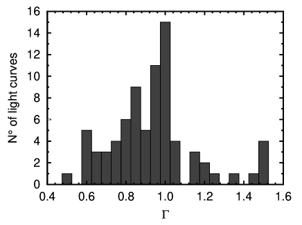
Figure 3: Histogram of the values of $\Gamma$.

There is no significant difference between the distributions without/with the factor $\Gamma$ (this is consistent with the fact that $\langle\Gamma\rangle=1$ with a small dispersion), so we present only results including this factor. Note that this holds for our particular DLC sample, for which $\langle\Gamma\rangle\approx 1$, but it will not be the case if control$-$comparison stars are not suitably selected (i.e. $\langle\Gamma\rangle\gg 1$). The histograms presented in Fig. 4 correspond to $\Delta m$, to $\Delta t$ in Fig. 5, to $n$ in Fig. 6 and to $\sigma_{2}$ in Fig. 7.

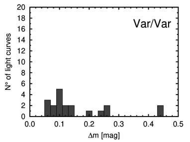
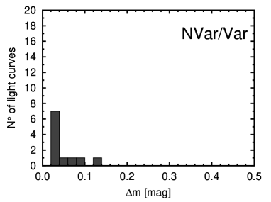
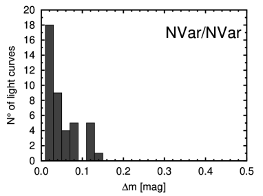
Figure 4: Histograms of $\Delta m$ for the cases: Var/Var, NVar/Var and NVar/NVar.

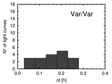
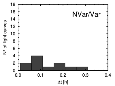
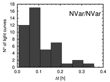
Figure 5: Histograms of $\Delta t$ for the cases: Var/Var, NVar/Var and NVar/NVar.

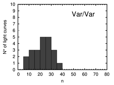
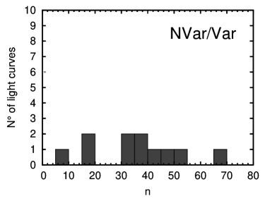
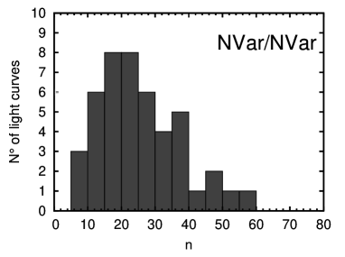
Figure 6: Histograms of $n$ for the cases: Var/Var, NVar/Var and NVar/NVar.

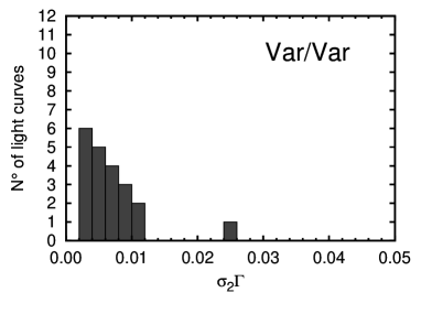
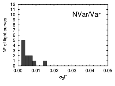
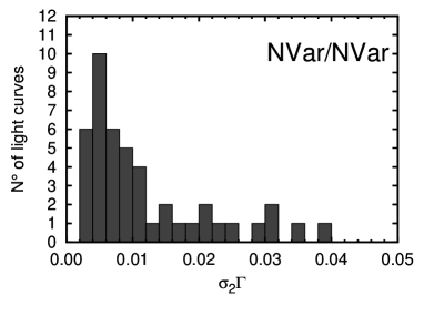
Figure 7: Histograms of weighted $\sigma_{2}$ (i.e. $\sigma_{2}\Gamma$) for the cases: Var/Var, NVar/Var and NVar/NVar.

Table 3: Results of the KS test. The columns show the variable considered; which distributions are compared; the KS statistical parameter $Z$; the maximum distance between distributions, $d$; and the area under the distribution of the statistical parameter $Z$ to the left, 1-prob.

Variable	Compared distributions	$Z$	$d$	1-prob
$\Delta m$	Var/Var versus NVar/Var	2.0409	0.727	0.999
	Var/Var versus NVar/NVar	2.5058	0.644	0.999
	NVar/Var versus NVar/NVar	0.6632	0.222	0.282
$\Delta t$	Var/Var versus NVar/Var	0.6373	0.227	0.211
	Var/Var versus NVar/NVar	1.6226	0.417	0.992
	NVar/Var versus NVar/NVar	1.3084	0.438	0.954
$n$	Var/Var versus NVar/Var	1.9146	0.682	0.999
	Var/Var versus NVar/NVar	0.7704	0.198	0.447
	NVar/Var versus NVar/NVar	1.5086	0.505	0.986
$\sigma_{2}$	Var/Var versus NVar/Var	1.2773	0.455	0.933
	Var/Var versus NVar/NVar	1.0350	0.266	0.790
	NVar/Var versus NVar/NVar	1.2367	0.414	0.931

3.5 Details on the distributions

In order to statistically study the behaviour observed in the histograms, we applied a goodness-of-fit Kolmogorov$-$Smirnov test (KS) to the data used to build the histograms. The results are presented in Table 3. The columns show the variable considered; the distributions compared; the KS statistical parameter $Z$; the maximum distance between distributions, $d$; and the area under the distribution of $Z$ to the left, 1-prob.

In the following, we analyse the results shown in Figs. 4$-$7, and quantified in Table 3.

DLC amplitude: the DLCs classified as non-variable with both tests (NVar/NVar), as well as those that change status depending on the criterion used (NVar/Var), show distributions strongly concentrated to small $\Delta m$ values (Fig. 4). The KS test gives a level of significance 1-prob$=0.282$; thus, it cannot be said that both distributions are statistically different. Both have a high peak at $\Delta m\approx 0.03$ mag, a value near the typical instrumental noise in light curves. Several of these light curves are identified as variable by the $F$ test, while none of them passes the $C$ criterion (see the Var/Var panel in Fig. 4).

DLCs with high $\Delta m$ values will thus tend to be classified as variable with both parameters, while the $F$ test, in particular, seems prone to classify as variable some DLCs with amplitudes very near to the rms error.

Elapsed time: DLCs classified as non-variable with both parameters have a broad distribution, with a peak around low values ($\Delta t$ $\leq 0.1$ h; Fig. 5). This peak is consistent with variations due to relatively rapid fluctuations of atmospheric conditions and photometric errors.

Regarding the distributions of DLCs classified as variable with the $F$ test (NVar/Var and Var/Var), they are wider, differing significantly from the NVar/NVar case. This agrees with the fact that a high value of $\Delta t$ tends to be more characteristic of curves that present a systematic variability as opposed to fast instrumental/atmospheric flickering. In those curves, where the instrumental noise is relatively low, this fact is more noticeable. While the $F$ test seems to be more sensitive to classify as variable curves with these characteristics, the KS test gives 1-prob$=0.211$ for the Var/Var versus NVar/Var histograms (Figs 5a and b), meaning that we cannot claim that the distributions are statistically different.

Number of observations: in the cases where the classification does not change (Var/Var and NVar/NVar, Figs 6a and c), the distributions are broad, peaking at $n\approx 20$, i.e. about the median number of data points in our DLCs. The KS test gives 1-prob$=0.447$ for the Var/Var versus NVar/NVar histograms. The NVar/Var case, in turn, shows a much flatter distribution, indicating some preference in favour of heavily sampled DLCs. This is usually the case of bright objects, for which exposure times are short (a few minutes), and photometric errors are usually smaller.

Dispersion of the control$-$comparison DLC: in those cases in which the state of variability is maintained (i.e., Var/Var and NVar/NVar; Figs 7a and c), we observe that the distributions of $\Gamma\sigma_{2}$ clump below $\sim 0.012$ mag. This implies DLCs with low instrumental dispersion, i.e. with high S/N ratio. The variability detection in these DLCs (non$-$detection in the case of NVar/NVar) is thus robust. However, for the NVar/NVar case, there is a tail of DLCs with $\Gamma\sigma_{2}\geq 0.02$ mag. This means low S/N ratio; hence, any intrinsic AGN variability of low amplitude would be masked by the, relatively, high noise.

The distribution of NVar/NVar cases is broader than that for Var/Var (the KS test gives a value 1-prob$=0.790$, i.e. it cannot be said that the Var/Var and NVar/NVar histograms are statistically different). This would imply a slightly larger sensitivity of the $F$ test to detect variability in noisy DLCs (or, from a different point of view, a higher tendency to produce false positives under low S/N conditions).

We also made an analysis of the light curves obtained after interchanging the roles of the comparison and control stars, in order to study how the choice of these stars could influence the statistical results. We applied both parameters to the DLCs, finding out that close to the 95 per cent of the light curves maintained their classifications with the $C$ criterion; meanwhile, for the $F$ test that percentage dropped to 85 per cent. This is consistent with the fact that the mean value of $\Gamma$ is close to $1$, with a low dispersion. However, again, $F$ seems more sensitive to systematics than $C$.

4 Inquiring into the $C$ criterion

As defined in Section 3.1, the parameter $C$ is the ratio between the standard deviations of two given distributions. The genesis of its use in AGN microvariability studies can be traced back to Carini et al. (1990) who proposed that the dispersion of the differential magnitudes of the control light curve could provide an estimator for the stability of the standard stars used in the data analysis, being a more reliable measure of the observational uncertainty than formal photometric errors. A further step was given by Jang & Miller (1995); they fitted both ‘object$-$comparison’ and ‘control$-$comparison’ light curves with straight lines and computed the standard deviations of the data points in each curve. The largest value, either from one or from the other light curve, was taken as a measure of the observational error. Note that this procedure removes any long-term variation in the light curves, while, at the same time, is insensitive to any ‘erratic, low$-$amplitude variation’ of the AGN (Carini et al., 1991). Jang & Miller (1997) explicitly use the 99 per cent CL for magnitude variations with amplitudes exceeding $2.576\,\sigma$, assuming a normal distribution. In Romero et al. (1999), an explicit definition for $C$ is given (equation 1), where the amplitude of the target$-$comparison DLC has been changed by its dispersion, in an attempt to compensate for the extreme sensibility of the Jang & Miller (1997) criterion to systematic (mostly type-I) errors (the practical reason for this choice is illustrated in Section 5). Thus, the parameter $C$ is the result of trying to improve the estimation of the data errors, providing a variability criterion as strong as possible against false positives arising from systematic errors.

However, we saw above that the $C$ criterion gives different results than the $F$ test. Since the $F$ test is firmly rooted in a statistical theoretical background, whereas the $C$ is a rather loosely grounded criterion (that eventually got to be considered as an actual test), we decided to carefully analyse the latter.

Putting aside for the moment the particular case of comparing light curves, in a general setup the goal of both the $C$ and the $F$ statistics is to compare the dispersions ($C$ criterion) or variances ($F$ test) of two samples, taken from unknown populations. Both carry out the comparison by rejecting (or not) the null hypothesis that both dispersions and variances are statistically the same. Let $C={\sigma_{1}}/{\sigma_{2}}$, and $F={\sigma_{1}^{2}}/{\sigma_{2}^{2}}$, where $\sigma_{1}$ and $\sigma_{2}$ are the dispersions being compared, with $\sigma_{1}>\sigma_{2}$ in the case of the $F$ statistic. We discard here any explicit scaling factor, because we are not computing results of the tests but comparing them, so the numerical values of the dispersions are irrelevant here.

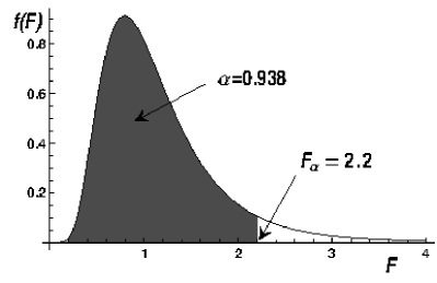
Figure 8: Example of a Fisher $F$ density distribution, here with $\nu_{1}=20$, $\nu_{2}=15$, i.e. the sample with the larger dispersion has 21 measurements, and the other one 16. The CL is chosen here as $\alpha=0.938$, which gives a value of $F_{\alpha}=2.2$. If it turns out that $F_{\rm obs}>F_{\alpha}$, the null hypothesis is rejected; otherwise, the null hypothesis is not rejected.

In order to make a theoretically based comparison between the methods, we recall here the procedure for the $F$ test. First, we have to choose a CL $\alpha$, that is, the complement of the probability that two variances will give by chance an $F$ value so large that the null hypothesis should be rejected. If, for example, one chooses 1 per cent as the above$-$mentioned probability, then $\alpha=0.99$. Secondly, the ‘degrees of freedom’ $\nu_{i}=n_{i}-1,i=1,2$ are computed, where $n_{i},i=1,2$ are the number of measurements of each sample. Thirdly, by using the probability density distribution of the statistical variable $F$ with $\nu_{1}$ and $\nu_{2}$ degrees of freedom, a value $F_{\alpha}$ is found, such that the area below the distribution mentioned before to the left of $F_{\alpha}$ be $\alpha$ (Fig. 8). Fourthly, a value $F_{\rm obs}=\sigma_{1}^{2}/\sigma_{2}^{2}$ is computed from the measurements, by using for each sample the usual formula

$$\sigma^{2}={1\over n-1}\sum_{i=1}^{n}(x_{i}-\mu)^{2},$$ (6)

where $n$ is the size of the sample, $x_{i}$ are the measurements, and $\mu$ is the mean of the sample, i.e., the sum of the measurements divided by $n$. Finally, $F_{\rm obs}$ is compared against $F_{\alpha}$. If $F_{\rm obs}>F_{\alpha}$, then the null hypothesis is rejected; otherwise, the null hypothesis is not rejected.

In turn, for the case of $C$ we have: first, the value $C_{\rm obs}$ is computed from the measurements, using the square root of equation (6) for each sample. Secondly, this value is (always) compared with the number 2.576, irrespective of the number of measurements. If $C>2.576$, the null hypothesis is rejected at a fixed 99.5 per cent CL.

So, the $C$ ‘test’ is not properly a statistical test. Tracing back the origin of the fixed numbers 2.576 and 99.5 per cent, it seems that they come from a standard rejection of a bad measurement procedure. According to this, given a set of measurements of a given quantity, we can always compute the variance of the sample by means of equation (6). Under the hypotheses that the measurements came with a Gaussian distribution of errors, and that the mean and the dispersion of the sample are good estimators of the true mean and dispersion of the population of measurements, one might discard those measurements that fall far enough from the mean of the sample because those measurements can be regarded highly improbable (some instrumental or operational error rather than to an error by chance). How far they should be from the mean in order to be discarded depends on the experiment; usually, this distance is measured in units of the dispersion of the sample. If this distance is taken as $1\sigma$, for instance, it is said that the measurement is rejected at a 68 per cent CL, because the area below a Gaussian inside the abscissae $x=\pm\sigma$ is approximately 0.68. But we may invert the argument and put forward a CL, finding what is the abscissa that gives that area. If one chooses, for example, 0.995 as the level, then one obtains $x=\pm 2.576\,\sigma$ ($C$ critical value).

In this way, $C$ is not a strict, theoretically supported statistical estimator . As we have seen, the rejection of a bad measurement works by comparing a given measurement with the mean of the distribution density of the measurements, and measuring the distance to that mean in terms of the dispersion of the distribution density of the measurements. In the $C$ criterion, however, a dispersion $\sigma_{1}$ is compared with a reference dispersion $\sigma_{2}$, as if this last value were the mean of the distribution density of dispersions, and the ratio $\sigma_{1}/\sigma_{2}$ becomes the distance, as if $\sigma_{2}$ were also the dispersion of the distribution density of dispersions. That is, for the $C$ criterion to work, $\sigma_{2}$ should be both the mean and the dispersion of the (unknown) distribution of dispersions. And, it should be pointed out that, whereas $C$ is strictly positive, and clearly the domain of a distribution density of dispersions is the set of positive reals plus zero, the $C$ criterion assumes a Gaussian distribution of dispersions, i.e., a domain equal to the set of all real numbers.

5 Results for field stars

To better understand the results presented in Section 3, we analysed the stability of the statistics using the field stars. To perform this, we considered all the selected stars in the frames, excluding the AGN, and we calculated the $C$ and $F$ parameters for all the DLCs using the same comparison and control stars as in the case of the corresponding AGN. By selected stars, we mean those (between 6 and 44 per field) making the set of candidates from which the comparison and control stars were finally chosen. We removed from this sample DLCs that were affected by saturation, cosmic rays, stars that were too close to the edge of the frames and any other evident defect. DLCs with $\Delta m\geq 0.4$ mag were also discarded; this should remove any remaining very ill-behaving DLC as well as known variables (e.g., star S in the field of 3C 279, a known variable with amplitude $>1$ mag; Raiteri et al., 1998). The original number of DLCs was $1039$, and after the cleaning process, we had 981 DLCs left for their study.

The first thing to note is that 16.9 per cent of the DLCs are found to be variable with the $F$ test, while this percentage drops to 9.5 per cent using the $C$ criterion (in both cases, the $\Gamma$ correction was applied). It is known (e.g. Ciardi et al., 2011, and references therein) that the fraction of variable stars in a given survey is a function of the survey parameters $-$time span and sampling of the observational series, photometric precision$-$, as well as the magnitudes, spectral types and luminosity classes of the stars. As a general guide, from ground-based data, Howell (2008) says that only 7 per cent of the stars are expected to vary at a 0.01 mag precision level. Ciardi et al. (2011), in turn, present a detailed variability analysis based on Kepler data, with a time resolution $\sim 30$ min. From their results, it can be inferred that the fraction of stars in our AGN fields (mostly located at relatively high Galactic latitudes) that vary at a level $>0.01$ mag within a few hours should be almost negligible $-$at most, well below 10 per cent.

It is clear that both criteria classify as ‘variable’ a larger$-$than$-$expected number of DLCs. However, this is particularly evident for the $F$ test: 76 out of 981 DLCs (7.7 per cent) change form NVar with the $C$ criterion to Var using the $F$ test (the converse holds for a negligible 0.3 per cent, i.e., just three DLCs, so we do not discuss this Var/NVar case). In order to further inquire into the reasons for this behaviour, we again analysed the distribution of the different parameters characterizing the DLCs, as was done for the AGN light curves. The general results are qualitatively similar to those presented in Sections 3.4 and 3.5. However, it is worth mentioning that the most significant differences between distributions (supported by the KS test) correspond to the ratio between the variability amplitude ($\Delta m$) and the scaled rms of the control light curve ($\Gamma\sigma_{2}$). While DLCs in the NVar/NVar case cluster at $\Delta m/(\Gamma\sigma_{2})\la 9$, those in the Var/Var case have a broad distribution from $\Delta m/(\Gamma\sigma_{2})\ga 9$ upwards; the NVar/Var case, in turn, shows a narrow distribution centred at $\Delta m/(\Gamma\sigma_{2})\simeq 9$. For the observed DLCs of the AGN sample, we obtained a similar result regarding the behaviour of the ratio $\Delta m/(\Gamma\sigma_{2})$ (also supported by the KS test).

This means that both parameters agree in their classification for almost all DLCs displaying variations with amplitudes above $\sim 9\,\Gamma\sigma_{2}$ (Var/Var), and for most DLCs with $\Delta m\la 9\,\Gamma\sigma_{2}$ (NVar/NVar), while a minor fraction of DLCs lying within a narrow range around the limiting value ($\Delta m\simeq 9\,\Gamma\sigma_{2}$) are classified as variable by the $F$ test and non-variable by the $C$ criterion. Thus, both parameters behave as sort of ‘$\sigma$-clipping’ criteria, but with different clipping factors. In this regard, it must be noted that if we apply the original criterion proposed by Jang & Miller (1997), i.e. $\Delta m>2.576\,\Gamma\sigma$, more than half the field stars DLCs (52.4 per cent) are classified as variable. On the other hand, if no weighting ($\Gamma$ factor) is applied, 20.7 per cent and 33.4 per cent of the stars are classified as variable with the $C$ criterion and $F$ test, respectively. Clearly, results from unweighted tests would be catastrophic, and we will no longer discuss them.

As a further comparison between different tests, we calculated the percentage of DLCs in each star field that resulted to be variable using the $C$ criterion and $F$ test, considering three different CLs: 95 per cent, 99 per cent, and 99.5 per cent. We found that the distributions (for both statistics and the three CLs) have a clear peak around 10 per cent, although, at the same CL, the histograms corresponding to the $F$ test extend to larger variability percentages. It is interesting to note that the distributions of $F_{99.5}$ and $C_{95}$, as shown in Fig. 9, are practically identical (a KS test gives a value of 1-prob$=0.001$). We interpret that, for our data, we have to relax the CL of the $C$ criterion to 95 per cent in order to obtain similar results as with the $F$ test at the 99.5 per cent CL.

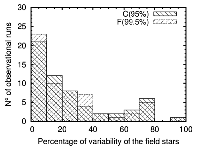
Figure 9: Distribution of percentages of stars per field that resulted variable using $C$ at 95 per cent$-$CL and $F$ at 99.5 per cent$-$CL.

It is now clear that the $F$ test is not working as expected (and neither does the $-$statistically ill founded$-$ $C$ criterion). However, this should not be surprising, since it is well$-$known that the $F$ test is particularly sensible to non-Gaussian errors (e.g. Wall & Jenkins, 2012), and photometric time series, unless taken by an absolutely perfect space telescope equipped with an absolutely perfect detector, will be affected by systematic error sources, adding a ‘red-noise’ (i.e. time$-$correlated at low frequencies) component. These sources of non-Gaussian distributed errors include flat-field imperfections, airmass variations, imperfect tracking, changing atmospheric conditions (seeing, transparency, scintillation), changing moonlight and airglow illumination, unnoticed cosmic rays, etc. Moreover, photometric errors usually correlate with those systematic effects, as e.g. when the S/N ratio drops due to changes in seeing or atmospheric transparency.

Any statistical test used to detect microvariability in AGN DLCs obtained with ground-based telescopes should thus be founded on solid theoretical bases and, at the same time, be able to deal both with random (i.e., photometric) and systematic (non-Gaussian) errors. In a forthcoming paper, we will further explore the performance of currently used tests by means of simulated observations. This will allow us to test variability tests under controlled situations, aiming at the selection of a test that is appropriate to deal with real observational issues.

6 Discussion

There are several works that have been dedicated to the study of statistical tools to detect microvariability in AGN. de Diego (2010) studied the $\chi^{2}$ test, the $F$ test for variances, the ANOVA test, and the $C$ criterion for a set of simulated light curves, concluding that the most robust methodologies are the ANOVA and $\chi^{2}$ tests, while the $F$ statistic is less powerful but still a reliable tool, and, finally, the $C$ criterion should be avoided because it is not a proper statistical test. Further analysis about these tests is presented in de Diego (2014), where a study of the Bartels and Runs non-parametric test was added. In that work, the author proposed that the best choices to detect microvariability in AGN light curves are the use of an ANOVA or an enhanced$-F$ test (in the latter, several comparison stars are used to define a combined variance, instead of using a single star). A continuation of this work was published by de Diego et al. (2015), where the enhanced-$F$ and the nested ANOVA tests were studied, concluding that these are the most powerful tests to detect photometric variations in DLCs, due to the increase in the power of the statistics, product of adding more comparison stars to the statistical analysis (the nested ANOVA test also requires some extra field stars, but fewer than in the enhanced-$F$ test).

It should be noted that, in these papers, the authors explicitly state that only photon shot$-$noise was considered for the light$-$curve simulations, while any systematic effect was ‘entirely disregarded’. So, despite their theoretical advantages, some of these tests may be impractical for dealing with real observations; moreover, if error distributions do not fulfil the assumptions on which those tests are based, their use should be discouraged or, at the very least, be taken with extreme care. In our case, we are working with DLCs with a rather small number of observations; this is a common situation, since AGN microvariability light curves are mostly limited to under $\sim 30-40$ points (e.g. Kumar & Gopal-Krishna, 2015). The need of a large number of points in light curves strongly limits the use of the $\chi^{2}$ test. The same applies to the ANOVA test: despite its claimed power to detect microvariability (de Diego, 2010; de Diego, 2014), this test is seldom used, because it requires a large number of data points too (Joshi et al., 2011); moreover, data grouping might be impractical for faint objects requiring relatively long integration times, and could lead to false results if data within a time span larger than the (unknown) variability time-scale are grouped. In fact, some doubtful results from the use of the ANOVA test in AGN microvariability studies (de Diego et al., 1998) have already been discussed in Romero et al. (1999). Regarding the nested ANOVA and the enhanced$-F$ tests, both tools require several comparison stars to perform optimally (de Diego et al., 2015), while having appropriately populated star fields around AGNs is more the exception than the rule. Villforth, Koekemoer & Grogin (2010), in turn, discuss the application of different tests to AGN light curves from space-based observations. They compare the $C$ criterion and the $\chi^{2}$ and $F$ tests using a sample of randomly generated light curves, concluding that the three tools show equal powers. However, when error measurements are themselves erroneous, $\chi^{2}$ has the highest power followed by $C$ and then $F$.

On the other hand, the use of tests specifically devised to deal with Gaussian errors may not be optimal to work with ground-based light curves, where atmospheric and instrumental effects produce correlated errors, with non-Gaussian distributions. In fact, even under pure random noise, errors in magnitude space will have asymmetric non-Gaussian distributions (e.g. Villforth et al., 2010). This is particularly relevant for the $\chi^{2}$ test, which requires that individual data points have accurately determined errors, with Gaussian distributions (e.g. Joshi et al., 2011); neither of these is always fulfilled by optical ground-based photometry. The $F$ test, in turn, does not behave as expected if error distributions are non-Gaussian (e.g. Wall & Jenkins, 2012). It is thus important to emphasize that $-$besides limitations typical of ground-based observations$-$ variability studies of AGNs usually have particular issues, like poorly sampled DLCs (due to low brightness of the source), and the availability of rather few field stars for differential photometry; these facts must be taken into account for the correct choice of the statistical analysis of the DLCs.

7 Summary and conclusions

In order to test the most widely used tests for AGN variability, we studied the $C$ and $F$ statistics with a large and homogeneous sample of real observational data. We worked with a sample of 39 southern AGNs observed with the 2.15m ‘Jorge Sahade’ telescope (CASLEO), San Juan, Argentina, obtaining 78 nightly differential photometry light curves, to which we applied the $C$ and $F$ statistics.

Besides which statistic is the better choice to analyse the behaviour of the DLCs, we want to point out that it is very important to use the weighted tests for the case of AGN differential photometry, because of the particular issues mentioned in the previous paragraph (see also Cellone et al., 2007, for a full discussion on this issue). We used the $\Gamma$ scale introduced by Howell & Jacoby (1986). There are cases in which the variability results change just because of not using this weight. Those cases are the ones in which $\Gamma$ is far from $1$ (i.e., the magnitudes of the comparison and/or control stars are not similar to the target’s magnitude).

From the results of applying the $C$ criterion and $F$ test to the sample, we found that, with respect to the DLC amplitude ($\Delta m$), $F$ results tend to classify as variable those DLCs with $\Delta m$ near the rms error, while for DLCs with high amplitude, both statistics tend to detect variability. For the elapsed time ($\Delta t$), DLCs with high values of $\Delta t$ are classified as variable, in agreement to the fact that this high value usually appears in light curves where systematic variability is observed. Both statistics seem to be robust in the detection (or non-detection) of variability when DLCs present low instrumental dispersion (0.012 mag), but if the dispersion of the ‘control$-$comparison’ light curve reaches values larger than 0.02 mag (some cases for the NVar/NVar histogram, Fig.7c), low-amplitude AGN variability could be masked due to the low S/N ratio in the DLC.

Taking a deeper look into the $C$ criterion, and comparing it with the $F$ test, we arrived at the conclusion that, even though the $C$ criterion cannot be considered as an actual statistical test, it could still be a useful parameter to detect variability, provided that the correct significance factor is chosen. In this way, we found that applying $C$ we may obtain rather more reliable variability results, especially for small amplitude and/or noisy DLCs.

Finally, a study of the behaviour of the field stars was made in order to analyse the stability of $C$ and $F$, excluding the AGN. From these new set of DLCs, we calculated the parameters involved in the statistics and the percentage of field stars that result variable for both $C$ and $F$. We found that, for the three CLs considered (95 per cent, 99 per cent and 99.5 per cent), both statistics show a peak around 10 per cent in their distributions, and comparing within the same CL, the $F$ test presents an extended distribution to larger variability percentages. We thus notice that the $F$ test tends to classify as variable a larger number of DLCs than the $C$ parameter, well above the expected number of variable stars in our fields. These variability results are clearly false positive results, possibly due to the inability of the $F$ test to deal with non-Gaussian distributed errors.

There has to be always a balance between the power of a given test (i.e. its ability to detect real variability) and its rate of false positives. Ultimately, the outcome of this balance should be dictated by astrophysical considerations, but this requires precise knowledge of each test’s behaviour under particular observational conditions.

This study is being completed carrying out a series of simulated observations, which involve differential photometry for several AGNs and comparison stars, immersed in a variety of distinct atmospheric conditions and several different observational situations. Results will be presented in a forthcoming paper.

Appendix A The distribution density function of the $D$ statistic

In order to determine whether two dispersions $\sigma_{1}$ and $\sigma_{2}$ are not statistically equivalent, a statistical test should be used. An equivalent test may be developed in which, instead of the ratio of the variances as in the $F$ test, the ratio of the dispersions is used, as in the $C$ parameter. In other words, we can convert the $C$ statistic into a statistical test. This new test should give no different results than the $F$ test. We will call it the $D$ test. With this new statistic, one follows the same steps as in the $F$ test: choosing a CL $\alpha$, computing the value $D_{\alpha}$ that leaves an area $\alpha$ to its left below the curve of the distribution density, finding the observed $D_{\rm obs}=\sigma_{1}/\sigma_{2}$ with $\sigma_{1}>\sigma_{2}$, and rejecting the null hypothesis if it happens that $D_{\rm obs}>D_{\alpha}$.

Suppose that, from a mother population with Gaussian probability density and (unknown) dispersion $\sigma$, a series of samples of $n$ members each are taken. For each sample, its sample variance $s^{2}$ can be computed as

$$s^{2}={1\over n-1}\sum_{i=1}^{n}(x_{i}-\mu)^{2},$$ (7)

where $x_{i}$ is the $i-$th member of the sample, and

$$\mu={1\over n}\sum_{i=1}^{n}x_{i}$$ (8)

is the mean of the sample. Hereafter, as a matter of convenience, we will use the number of degrees of freedom $\nu=n-1$ instead of the number of members $n$. The sample variances $s^{2}$ of the different samples have their own probability density distribution $f(s^{2})$, given by (Kendall & Stuart, 1969)

$$f(s^{2}\mid\nu,\sigma)=\left(\nu\over 2\right)^{\nu\over 2}{(s^{2})^{\nu/2-1}\over\sigma^{\nu}\Gamma(\nu/2)}\exp\left(-{\nu\over 2}{s^{2}\over\sigma^{2}}\right),$$ (9)

which depends on the parameters $\nu$ and $\sigma$. Taking into account that ${\rm d}(s^{2})=2s\,{\rm d}s$, it is easy to find the probability density distribution $g(s)$ of the sample dispersions $s$:

$$g(s\mid\nu,\sigma)={\nu^{\nu\over 2}\over 2^{\nu/2-1}}{s^{\nu-1}\over\sigma^{\nu}\Gamma(\nu/2)}\exp\left(-{\nu\over 2}{s^{2}\over\sigma^{2}}\right),$$ (10)

Now, given the distributions $g(s_{1}|\nu_{1},\sigma_{1})$ and $g(s_{2}|\nu_{2},\sigma_{2})$ of the dispersions of two set of samples, each with its own number of degrees of freedom $\nu_{1}$ and $\nu_{2}$, and maybe taken from different mother populations with true dispersions $\sigma_{1}$ and $\sigma_{2}$, one can find the distribution of their quotient $D=s_{1}/s_{2}$ as (Kendall & Stuart, 1969, sect. 11.6)

$$h(D\mid\nu_{1},\nu_{2},\sigma_{1},\sigma_{2})=$$ (11)

$$= \int_{0}^{\infty}g(Dx\mid\nu_{1}+1,\sigma_{1})g(x\mid\nu_{2}+1,\sigma_{2})x\,{\rm d}x$$

$$= 2{\Gamma({\nu_{1}+\nu_{2}\over 2})\over\Gamma({\nu_{1}\over 2})\Gamma({\nu_{2}\over 2})}{\nu_{1}^{\nu_{1}/2}\nu_{2}^{\nu_{2}/2}\sigma_{1}^{\nu_{2}}\sigma_{2}^{\nu_{1}}D^{\nu_{1}-1}\over(\nu_{2}\sigma_{1}^{2}+D^{2}\nu_{1}\sigma_{2}^{2})^{(\nu_{1}+\nu_{2})/2}}.$$

However, this result is completely useless because we do not know the true dispersions $\sigma_{1}$ and $\sigma_{2}$. But, if the mother population of both sets of samples is the same, or both sets come from populations with the same dispersion (i.e. $\sigma_{1}=\sigma_{2}\equiv\sigma$), then we have that the probability density distribution of the ratio $D$ is

$$h(D\mid\nu_{1},\nu_{2})=2{\Gamma({\nu_{1}+\nu_{2}\over 2})\over\Gamma({\nu_{1}\over 2})\Gamma({\nu_{2}\over 2})}{\nu_{1}^{\nu_{1}/2}\nu_{2}^{\nu_{2}/2}D^{\nu_{1}-1}\over(\nu_{2}+D^{2}\nu_{1})^{(\nu_{1}+\nu_{2})/2}},$$ (12)

which is independent of the true dispersion. This turns out to be the important point: this distribution is then ready to be used in a statistical test. In particular, since it is the result of assuming $\sigma_{1}=\sigma_{2}$, the $D$ test null hypothesis is that both $s_{1}$ and $s_{2}$ are statistically equivalent.

If the distribution equation (12) is compared with the well$-$known distribution for the $F$ statistic,

$$f(F\mid\nu_{1},\nu_{2})={\Gamma({\nu_{1}+\nu_{2}\over 2})\over\Gamma({\nu_{1}\over 2})\Gamma({\nu_{2}\over 2})}{\nu_{1}^{\nu_{1}/2}\nu_{2}^{\nu_{2}/2}F^{\nu_{1}/2-1}\over(\nu_{2}+F\nu_{1})^{(\nu_{1}+\nu_{2})/2}},$$ (13)

we see that they are the same distribution, only expressed with different variables, i.e. $h(D){\rm d}D=f(F){\rm d}F$ with $F=D^{2}$. Thus, using the $D$ test of dispersions gives exactly the same results as using the $F$ test of variances.

References

- Abdo et al. (2010) Abdo A. A., Ackermann M., Ajello M., Allafort A., Antolini E., Atwood W. B., Axelsson M., Baldini L., Ballet J., Barbiellini G., Bastieri D., Baughman B. M., Bechtol K., Bellazzini R., Berenji B., Blandford R. D., 2010, ApJ, 715, 429
- Ackermann et al. (2015) Ackermann M., Ajello M., Atwood W. B., Baldini L., Ballet J., Barbiellini G., Bastieri D., Becerra Gonzalez J., Bellazzini R., Bissaldi E., Blandford R. D., Bloom E. D., Bonino R., Bottacini E., Brandt T. J., 2015, ApJ, 810, 14
- Andruchow et al. (2003) Andruchow I., Cellone S. A., Romero G. E., Dominici T. P., Abraham Z., 2003, A&A, 409, 857
- Andruchow et al. (2005) Andruchow I., Romero G. E., Cellone S. A., 2005, A&A, 442, 97
- Carini et al. (1990) Carini M. T., Miller H. R., Goodrich B. D., 1990, AJ, 100, 347
- Carini et al. (1991) Carini M. T., Miller H. R., Noble J. C., Sadun A. C., 1991, AJ, 101, 1196
- Carini et al. (2007) Carini M. T., Noble J. C., Taylor R., Culler R., 2007, AJ, 133, 303
- Cellone et al. (2007) Cellone S. A., Romero G. E., Araudo A. T., 2007, MNRAS, 374, 357
- Cellone et al. (2000) Cellone S. A., Romero G. E., Combi J. A., 2000, AJ, 119, 1534
- Ciardi et al. (2011) Ciardi D. R., von Braun K., Bryden G., van Eyken J., Howell S. B., Kane S. R., Plavchan P., Ramírez S. V., Stauffer J. R., 2011, AJ, 141, 108
- de Diego (2010) de Diego J. A., 2010, AJ, 139, 1269
- de Diego (2014) de Diego J. A., 2014, AJ, 148, 93
- de Diego et al. (1998) de Diego J. A., Dultzin-Hacyan D., Ramirez A., Benitez E., 1998, ApJ, 501, 69
- de Diego et al. (2015) de Diego J. A., Polednikova J., Bongiovanni A., Pérez García A. M., De Leo M. A., Verdugo T., Cepa J., 2015, AJ, 150, 44
- Howell (2008) Howell S. B., 2008, Astron. Nachr., 329, 259
- Howell & Jacoby (1986) Howell S. B., Jacoby G. H., 1986, PASP, 98, 802
- Howell et al. (1988) Howell S. B., Mitchell K. J., Warnock A., 1988, AJ, 95, 247
- Jang & Miller (1995) Jang M., Miller H. R., 1995, ApJ, 452, 582
- Jang & Miller (1997) Jang M., Miller H. R., 1997, AJ, 114, 565
- Joshi et al. (2011) Joshi R., Chand H., Gupta A. C., Wiita P. J., 2011, MNRAS, 412, 2717
- Kendall & Stuart (1969) Kendall M. G., Stuart A., 1969, The Advanced Theory of Statistics, Vol. 1, 3rd edn.. Griffin, London
- Kesteven et al. (1976) Kesteven M. J. L., Bridle A. H., Brandie G. W., 1976, AJ, 81, 919
- Kumar & Gopal-Krishna (2015) Kumar P., Gopal-Krishna C. H., 2015, MNRAS, 448, 1463
- Miller et al. (1989) Miller H. R., Carini M. T., Goodrich B. D., 1989, Nature, 337, 627
- Raiteri et al. (1998) Raiteri C. M., Villata M., Lanteri L., Cavallone M., Sobrito G., 1998, A&AS, 130, 495
- Ramírez et al. (2009) Ramírez A., de Diego J. A., Dultzin D., González-Pérez J.-N., 2009, AJ, 138, 991
- Ramírez et al. (2004) Ramírez A., de Diego J. A., Dultzin-Hacyan D., González-Pérez J. N., 2004, A&A, 421, 83
- Richards et al. (2011) Richards J. L., Max-Moerbeck W., Pavlidou V., King O. G., Pearson T. J., Readhead A. C. S., Reeves R., Shepherd M. C., Stevenson M. A., Weintraub L. C., Fuhrmann L., Angelakis E., Zensus J. A., Healey S. E., Romani R. W., 2011, ApJS, 194, 29
- Romero et al. (1999) Romero G. E., Cellone S. A., Combi J. A., 1999, A&AS, 135, 477
- Romero et al. (2000) Romero G. E., Cellone S. A., Combi J. A., 2000, A&A, 360, L47
- Romero et al. (2002) Romero G. E., Cellone S. A., Combi J. A., Andruchow I., 2002, A&A, 390, 431
- Romero et al. (1994) Romero G. E., Combi J. A., Colomb F. R., 1994, A&A, 288, 731
- Véron-Cetty & Véron (2010) Véron-Cetty M.-P., Véron P., 2010, A&A, 518, A10
- Villforth et al. (2010) Villforth C., Koekemoer A. M., Grogin N. A., 2010, ApJ, 723, 737
- Wall & Jenkins (2012) Wall J. V., Jenkins C. R., 2012, Practical Statistics for Astronomers.. Cambridge Univ. Press, Cambridge, UK
- Zibecchi et al. (2011) Zibecchi L., Andruchow I., Cellone S. A., Romero G. E., Combi J. A., 2011, Bol. Asociacion. Argentina Astron., 54, 325